CS151 Complexity Theory Lecture 6 April 15, 2015.
56
CS151 Complexity Theory Lecture 6 April 15, 2015
-
Upload
preston-black -
Category
Documents
-
view
223 -
download
3
Transcript of CS151 Complexity Theory Lecture 6 April 15, 2015.

CS151Complexity Theory
Lecture 6
April 15, 2015
April 15, 2015 2
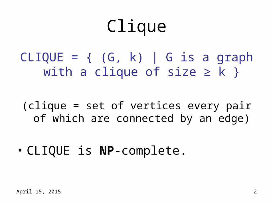
Clique
CLIQUE = { (G, k) | G is a graph with a clique of size ≥ k }
(clique = set of vertices every pair of which are connected by an edge)
• CLIQUE is NP-complete.

April 15, 2015 3
Circuit lower bounds
• We think that NP requires exponential-size circuits.
• Where should we look for a problem to attempt to prove this?
• Intuition: “hardest problems” – i.e., NP-complete problems
April 15, 2015 4
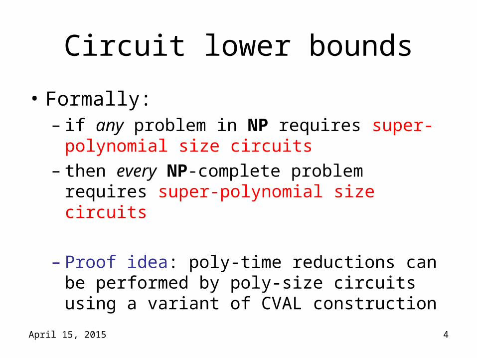
Circuit lower bounds
• Formally: – if any problem in NP requires super-
polynomial size circuits– then every NP-complete problem requires
super-polynomial size circuits
– Proof idea: poly-time reductions can be performed by poly-size circuits using a variant of CVAL construction

April 15, 2015 5
Monotone problems
• Definition: monotone language = language
L {0,1}*
such that x L implies x’ L for all x ¹ x’.
– flipping a bit of the input from 0 to 1 can only change the output from “no” to “yes” (or not at all)

April 15, 2015 6
Monotone problems
• some NP-complete languages are monotone– e.g. CLIQUE (given as adjacency matrix):
– others: HAMILTON CYCLE, SET COVER…– but not SAT, KNAPSACK…

April 15, 2015 7
Monotone circuits
A restricted class of circuits:
• Definition: monotone circuit = circuit whose gates are ANDs (), ORs (), but no NOTs
• can compute exactly the monotone fns.– monotone functions closed under AND, OR

April 15, 2015 8
Monotone circuits
• A question:
Do all
poly-time computable monotone functions
have
poly-size monotone circuits?
– recall: true in non-monotone case

April 15, 2015 9
Monotone circuits
A monotone circuit for CLIQUEn,k
• Input: graph G = (V,E) as adj. matrix, |V|=n– variable xi,j for each possible edge (i,j)
• ISCLIQUE(S) = monotone circuit that = 1
iff S V is a clique: i,j S xi,j
• CLIQUEn,k computed by monotone circuit:
S V, |S| = k ISCLIQUE(S)

April 15, 2015 10
Monotone circuits
• Size of this monotone circuit for CLIQUEn,k:
• when k = n1/4, size is approximately:
n k
k 2
1/ 41/ 4
n 1/ 4n
4
2
1/
nn
2n
n

April 15, 2015 11
Monotone circuits
• Theorem (Razborov 85): monotone circuits for CLIQUEn,k with k = n1/4 must have size at least
2Ω(n1/8).
• Proof: – rest of lecture

April 15, 2015 12
Proof idea
• “method of approximation”
• suppose C is a monotone circuit for CLIQUEn,k
• build another monotone circuit CC that “approximates” C gate-by-gate

April 15, 2015 13
Proof idea
• on test collection of positive/negative instances of CLIQUEn,k:
– local property: few errors at each gate– global property: many errors on test collection
• Conclude: C has many gates

April 15, 2015 14
Notation
• input: graph G = (V, E)• variable xj,k for each potential edge (j, k)• CC(X1, X2, … Xm), where Xi V, means:
i ( j,k Xi xj,k) *
• For example: CC(X1, X2, … Xm) where the Xi range over all k-subsets of V– this is the obvious monotone circuit for CLIQUEn,k
from a previous slide.
*[CC( ) = 0; ( j,k ; xj,k) = 1]

April 15, 2015 15
Preview
• approximate circuit CC(X1, X2, … Xm)
• n = # nodes
• k = n1/4 = size of clique
• h = n1/8 = max. size of subsets Xi
– this is “global property” that ensures lots of errors
– many graphs G with no k-cliques, but clique on Xi of size h
G
Xi
April 15, 2015 16
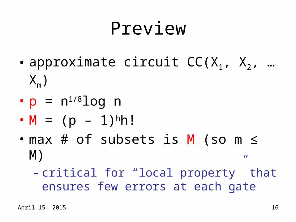
Preview
• approximate circuit CC(X1, X2, … Xm)
• p = n1/8log n
• M = (p – 1)hh!
• max # of subsets is M (so m ≤ M)– critical for “local property” that ensures few
errors at each gate
April 15, 2015 17
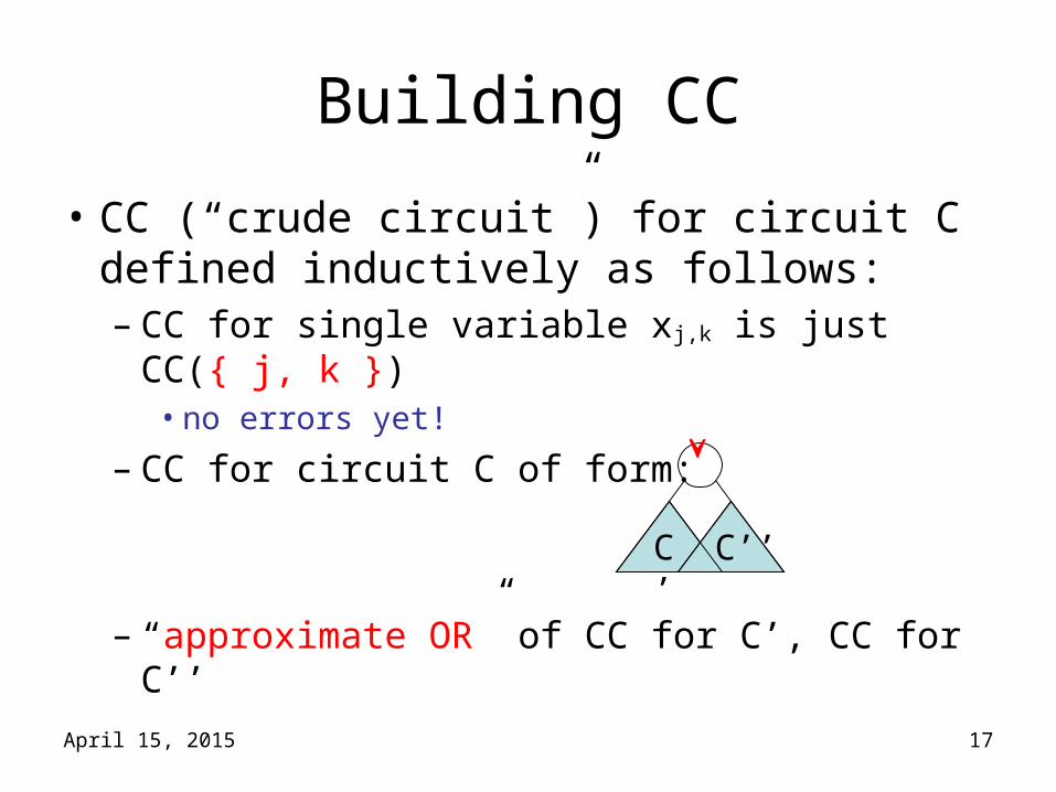
Building CC
• CC (“crude circuit”) for circuit C defined inductively as follows:– CC for single variable xj,k is just CC({ j, k })
• no errors yet!
– CC for circuit C of form:
– “approximate OR” of CC for C’, CC for C’’
C’
C’’

April 15, 2015 18
Building CC
– CC for circuit C of form:
– “approximate AND” of CC for C’, CC for C’’
– “approximate OR” and “approximate AND” steps introduce errors
C’
C’’

April 15, 2015 19
Approximate OR
CC(X1,X2,…Xm’) CC(Y1,Y2,…Ym’’)
• exact OR:
CC(X1,X2,…Xm’,Y1,Y2,…Ym’’)
– set sizes still ≤ h– may be up to 2M sets; need to reduce to M
C’
C’’

April 15, 2015 20
Approximate OR
– throw away sets? bad:many errors– throw away overlapping sets? – better
– throw away special configuration of overlapping sets – best

April 15, 2015 21
Sunflowers
• Definition: (h, p)-sunflower is a family of p sets (“petals”) each of size at most h, such that intersection of every pair is a subset S (the “core”).

April 15, 2015 22
Sunflowers
Lemma (Erdös-Rado): Every family of more than M = (p-1)hh! sets, each of size at most h, contains an (h, p)-sunflower.
• Proof: – not hard– in Papadimitriou, elsewhere
April 15, 2015 23
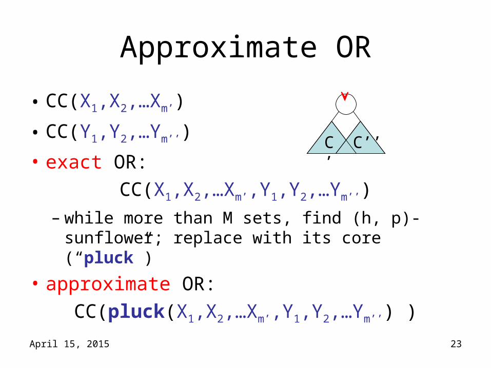
Approximate OR
• CC(X1,X2,…Xm’)
• CC(Y1,Y2,…Ym’’)
• exact OR:
CC(X1,X2,…Xm’,Y1,Y2,…Ym’’)
– while more than M sets, find (h, p)-sunflower; replace with its core (“pluck”)
• approximate OR:
CC(pluck(X1,X2,…Xm’,Y1,Y2,…Ym’’) )
C’
C’’

April 15, 2015 24
Approximate AND
• CC(X1,X2,…Xm’)
• CC(Y1,Y2,…Ym’’)
• (close to) exact AND:
CC( {(Xi Yj) : 1 ≤ i ≤ m’, 1 ≤ j ≤ m’’} )– some sets may be larger than h; discard them– may be up to M2 sets. While > M sets, find (h, p)-
sunflower; replace with its core (“pluck”)
• approximate AND:
CC( pluck ( {(XiYj) : |XiYj| ≤ h } ))
C’
C’’

April 15, 2015 25
Test collection
• Positive instances: all graphs G on n nodes with a k-clique and no other edges.
G
April 15, 2015 26
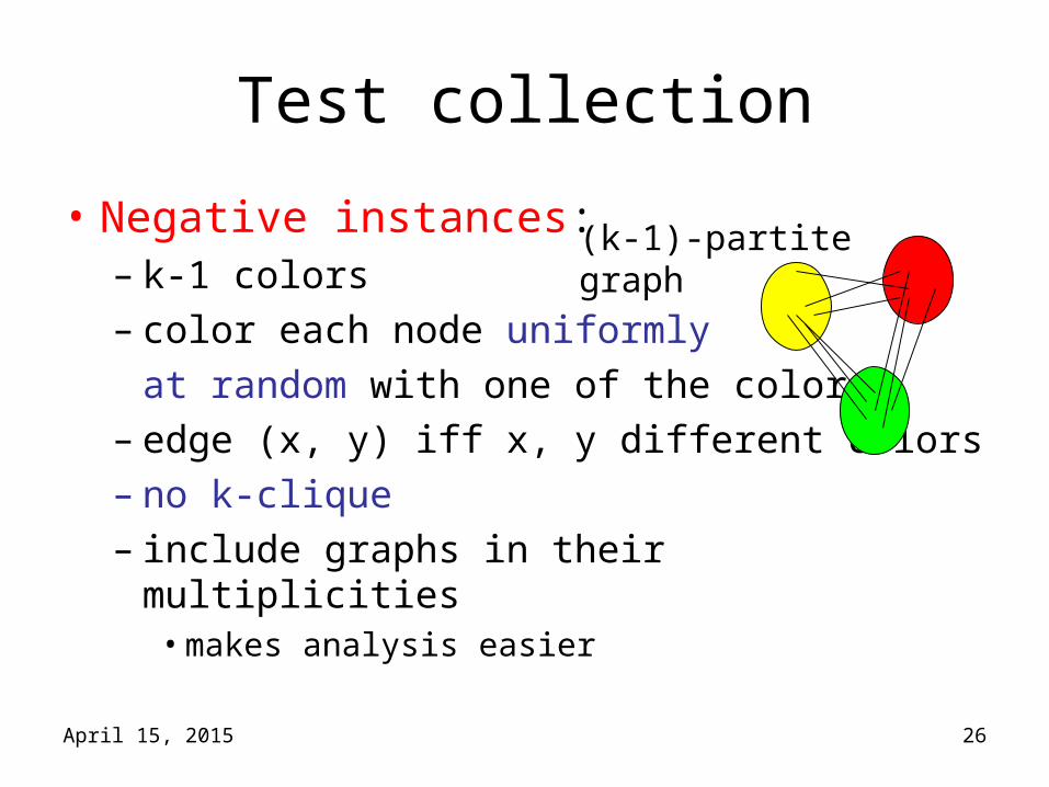
Test collection
• Negative instances:– k-1 colors– color each node uniformly
at random with one of the colors– edge (x, y) iff x, y different colors– no k-clique– include graphs in their multiplicities
• makes analysis easier
(k-1)-partite graph

April 15, 2015 27
“Local” analysis
• “false positive”:– negative example– gate is supposed to output 0, but our CC
outputs 1
Lemma: each approximation step introduces at most M2(k-1)n/2p false positives.

April 15, 2015 28
“Local” analysis
• Proof:– case 1: OR
CC(X1,X2,…Xm’) CC(Y1,Y2,…Ym’’)
CC(pluck(X1,X2,…Xm’,Y1,Y2,…Ym’’))
– given “plucking”: replace Z1… Zp with Z
– bad case: clique on Z, and each petal is missing at least one edge
C’
C’’

April 15, 2015 29
“Local” analysis
– what is the probability of a repeated color in each Zi
but no repeated colors in Z?
Pr[R(Z1)R(Z2)…R(Zp) R(Z)]
≤ Pr[R(Z1)R(Z2)…R(Zp)|R(Z)]
(definition of conditional probability)
= i Pr[R(Zi) | R(Z)]
(independent events given no repeats in Z)
≤ i Pr[R(Zi)]
(obviously larger)
event R(S) = repeated colors in S
April 15, 2015 30
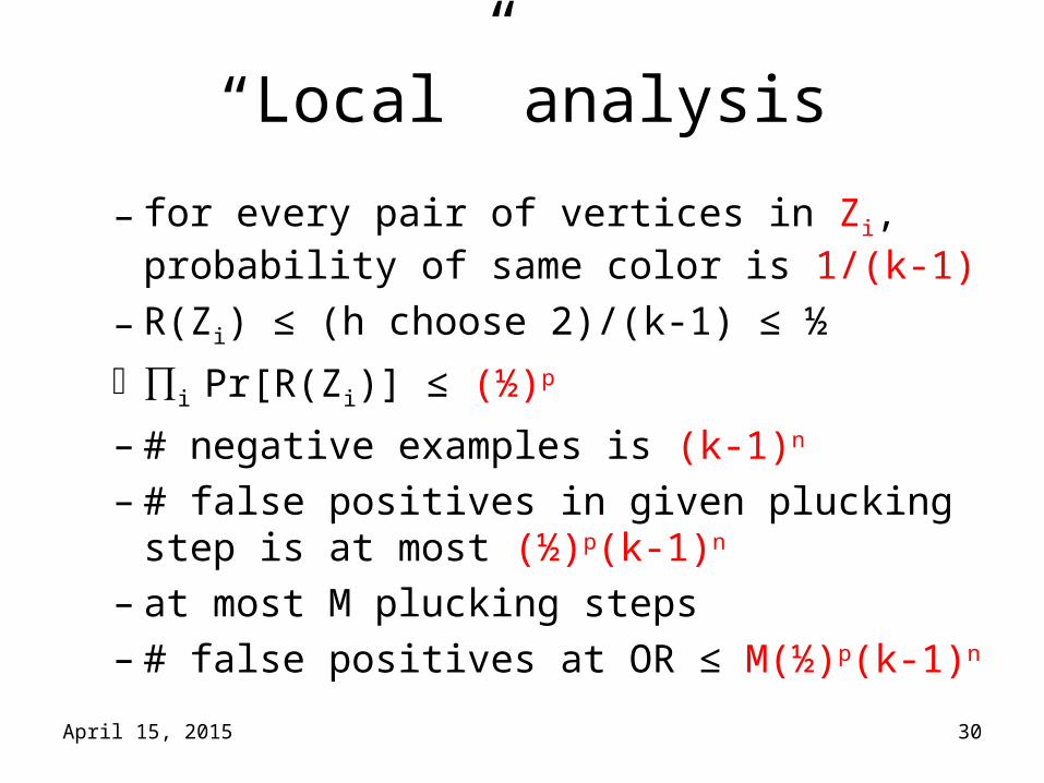
“Local” analysis
– for every pair of vertices in Zi, probability of same color is 1/(k-1)
– R(Zi) ≤ (h choose 2)/(k-1) ≤ ½
i Pr[R(Zi)] ≤ (½)p
– # negative examples is (k-1)n
– # false positives in given plucking step is at most (½)p(k-1)n
– at most M plucking steps– # false positives at OR ≤ M(½)p(k-1)n

April 15, 2015 31
“Local” analysis
– case 2: AND
CC(X1,X2,…Xm’) CC(Y1,Y2,…Ym’’)
CC(pluck( {(XiYj) : |XiYj| ≤ h } ))
– discarding sets (XiYj) larger than h can only make circuit accept fewer examples
• no false positives here
C’
C’’
April 15, 2015 32
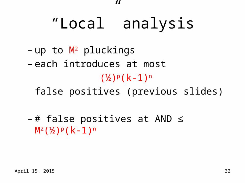
“Local” analysis
– up to M2 pluckings– each introduces at most
(½)p(k-1)n
false positives (previous slides)
– # false positives at AND ≤ M2(½)p(k-1)n

April 15, 2015 33
“Local” analysis
• “false negative”: – positive example; – gate is supposed to output 1, but our CC
outputs 0
Lemma: each approximation step introduces at most
false negatives.
2 n h 1M
k h 1

April 15, 2015 34
“Local” analysis
• Proof:– Case 1: OR– plucking can only make circuit accept more
examples• no false negatives here.
– Case 2: AND
CC(X1,X2,…Xm’) CC(Y1,Y2,…Ym’’)
CC(pluck( {(XiYj) : |XiYj| ≤ h } ))
• for positive examples: clique on Xi and clique on Yj ) clique on Xi[Yj (no false negatives until discard Xi[Yj sets)
C’
C’’

April 15, 2015 35
“Local” analysis
– discarding set Z = (XiYj) larger than h may introduce false negatives
– any clique that includes Z is a problem; there are at most
such positive examples, since |Z|>h– at most M2 such deletions– we’ve seen plucking doesn’t matter
n Z n h 1
k Z k h 1
April 15, 2015 36
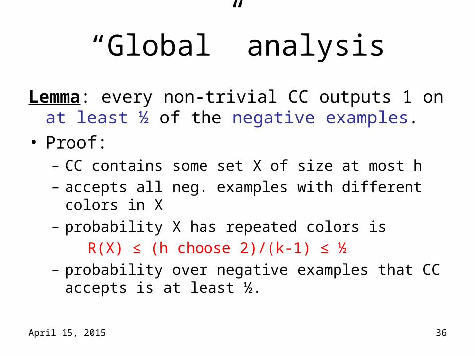
“Global” analysis
Lemma: every non-trivial CC outputs 1 on at least ½ of the negative examples.
• Proof: – CC contains some set X of size at most h– accepts all neg. examples with different colors in X– probability X has repeated colors is
R(X) ≤ (h choose 2)/(k-1) ≤ ½ – probability over negative examples that CC accepts is
at least ½.
April 15, 2015 37
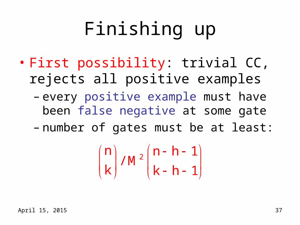
Finishing up
• First possibility: trivial CC, rejects all positive examples– every positive example must have been false
negative at some gate– number of gates must be at least:
2n n h 1
/ Mk k h 1

April 15, 2015 38
Finishing up
• Second possibility: CC accepts at least ½ of negative examples– every negative example must have been false
positive at some gate– number of gates must be at least:
pn 2 n1(k 1) / M 2 (k 1)
2
April 15, 2015 39
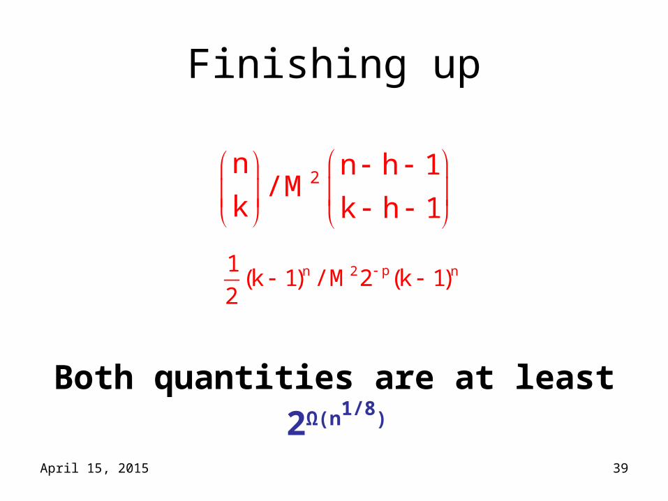
Finishing up
Both quantities are at least 2Ω(n1/8)
2n n h 1
/ Mk k h 1
pn 2 n1(k 1) / M 2 (k 1)
2

April 15, 2015 40
Conclusions
• A question (true in non-monotone case):
Do all
poly-time computable monotone functions
have
poly-size monotone circuits?
• if yes, then we would have just proved P ≠ NP – why?

April 15, 2015 41
Conclusions
• unfortunately, answer is no
• Razborov later showed similar (super-polynomial) lower bound for MATCHING, which is in P…

April 15, 2015 42
Next up… randomness
• 3 examples of the power of randomness – communication complexity– polynomial identity testing– complexity of finding unique solutions
• randomized complexity classes

April 15, 2015 43
1. Communication complexity
• Goal: compute f(x, y) while communicating as few bits as possible between Alice and Bob
• count number of bits exchanged (computation free)
• at each step: one party sends bits that are a function of held input and received bits so far
two parties: Alice and Bob
function f:{0,1}n x {0,1}n {0,1}
Alice holds x {0,1}n; Bob holds y {0,1}n
April 15, 2015 44
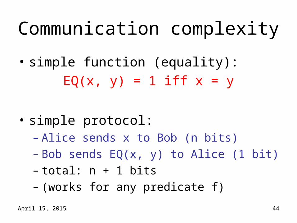
Communication complexity
• simple function (equality):
EQ(x, y) = 1 iff x = y
• simple protocol:– Alice sends x to Bob (n bits)– Bob sends EQ(x, y) to Alice (1 bit)– total: n + 1 bits– (works for any predicate f)

April 15, 2015 45
Communication complexity
• Can we do better?– deterministic protocol?– probabilistic protocol?
• at each step: one party sends bits that are a function of held input and received bits so far and the result of some coin tosses
• required to output f(x, y) with high probability over all coin tosses

April 15, 2015 46
Communication complexity
Theorem: no deterministic protocol can compute EQ(x, y) while exchanging fewer than n+1 bits.
• Proof:– “input matrix”:
X = {0,1}n
Y = {0,1}n
f(x,y)

April 15, 2015 47
Communication complexity
– assume 1 bit sent at a time, alternating (same proof works in general setting)
– A sends 1 bit depending only on x:
X = {0,1}n
Y = {0,1}n
inputs x causing A to send 1
inputs x causing A to send 0

April 15, 2015 48
Communication complexity
– B sends 1 bit depending only on y and received bit:
X = {0,1}n
Y = {0,1}n
inputs y causing B to send 1
inputs y causing B to send 0

April 15, 2015 49
Communication complexity
– at end of protocol involving k bits of communication, matrix is partitioned into at most 2k combinatorial rectangles
– bits sent in protocol are the same for every input (x, y) in given rectangle
– conclude: f(x,y) must be constant on each rectangle
April 15, 2015 50
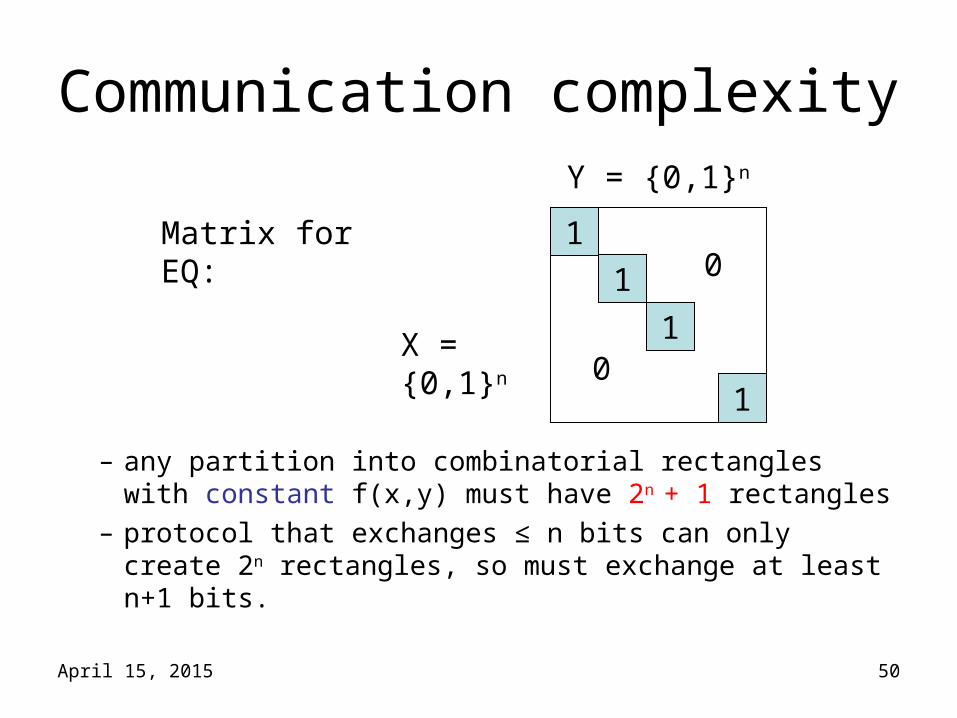
Communication complexity
– any partition into combinatorial rectangles with constant f(x,y) must have 2n + 1 rectangles
– protocol that exchanges ≤ n bits can only create 2n rectangles, so must exchange at least n+1 bits.
X = {0,1}n
Y = {0,1}n
1
1
1
10
0Matrix for EQ:

April 15, 2015 51
Communication complexity
• protocol for EQ employing randomness?– Alice picks random prime p in {1...4n2}, sends:
• p • (x mod p)
– Bob sends: • (y mod p)
– players output 1 if and only if:
(x mod p) = (y mod p)

April 15, 2015 52
Communication complexity
– O(log n) bits exchanged– if x = y, always correct– if x ≠ y, incorrect if and only if:
p divides |x – y|– # primes in range is ≥ 2n– # primes dividing |x – y| is ≤ n– probability incorrect ≤ 1/2
Randomness gives an exponential advantage!!

April 15, 2015 53
2. Polynomial identity testing
• Given: polynomial p(x1, x2, …, xn) as arithmetic formula (fan-out 1):
-
*
x1 x2
*
+ -
x3 … xn
*• multiplication (fan-in 2)
• addition (fan-in 2)
• negation (fan-in 1)

April 15, 2015 54
Polynomial identity testing
• Question: Is p identically zero?– i.e., is p(x) = 0 for all x Fn – (assume |F| larger than degree…)
• “polynomial identity testing” because given two polynomials p, q, we can check the identity p q by checking if (p – q) 0
April 15, 2015 55
Polynomial identity testing
• try all |F|n inputs? – may be exponentially many
• multiply out symbolically, check that all coefficients are zero?– may be exponentially many coefficients
• can randomness help?– i.e., flip coins, allow small probability of wrong
answer
April 15, 2015 56
Polynomial identity testing
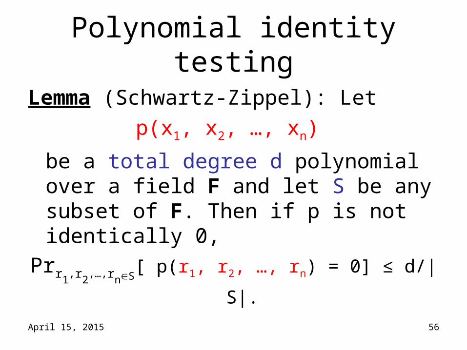
Lemma (Schwartz-Zippel): Let
p(x1, x2, …, xn)
be a total degree d polynomial over a field F and let S be any subset of F. Then if p is not identically 0,
Prr1,r2,…,rnS[ p(r1, r2, …, rn) = 0] ≤ d/|S|.