CS145: Probability & Computing - Brown...
19
CS145: Probability & Computing Lecture 4: Independence, Classification, Discrete Random Variables Instructor: Eli Upfal Brown University Computer Science Figure credits: Bertsekas & Tsitsiklis, Introduction to Probability, 2008 Pitman, Probability, 1999
Transcript of CS145: Probability & Computing - Brown...
CS145: Probability & ComputingLecture 4: Independence,
Classification, Discrete Random VariablesInstructor: Eli Upfal
Brown University Computer Science
Figure credits: Bertsekas & Tsitsiklis, Introduction to Probability, 2008
Pitman, Probability, 1999
CS145: Lecture 4 OutlineØ Independence and Conditional IndependenceØBayes’ Rule and ClassificationØDiscrete random variables
Independence of Two Events
LECTURE 2 Review of probability models
• Readings: Sections 1.3-1.4 • Sample space
– Mutually exclusiveCollectively exhaustive
Lecture outline– Right granularity
• Review • Event: Subset of the sample space
• Conditional probabilityAllocation of probabilities to events
• Three important tools:•
1. P(A) 0
– Multiplication rule 2. P() = 1
3. If– Total probability theorem A B = Ø,then P(A B) = P(A) + P(B)
– Bayes’ rule3’. If A1, A2, . . . are disjoint events, then:
P(A1 A2 · · · ) = P(A1) + P(A2) + · · ·
• Problem solving:
– Specify sample space
– Define probability law
– Identify event of interest
– Calculate...
Conditional probability Die roll example
4A
3Y = Second
B roll
2
1
• P(A | B) = probability of A,that B occurred 1 2 3
given 4
is our new universe X– B = First roll
• Definition: Assuming P(B) = 0, • Let B be the event: min(X, Y ) = 2
P(AP(A B) =
B)| • Let M = max(X, Y )
P(B)
P(A | B) undefined if P(B) = 0 • P(M = 1 | B) =
• P(M = 2 | B) =
1
A B
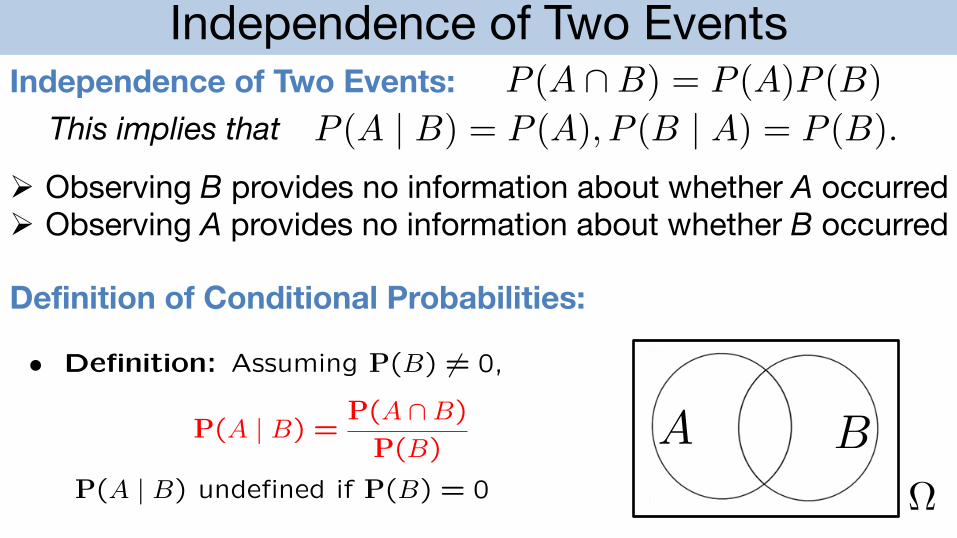
Definition of Conditional Probabilities:
Independence of Two Events: P (A \B) = P (A)P (B)P (A | B) = P (A), P (B | A) = P (B).This implies that
Ø Observing B provides no information about whether A occurredØ Observing A provides no information about whether B occurred
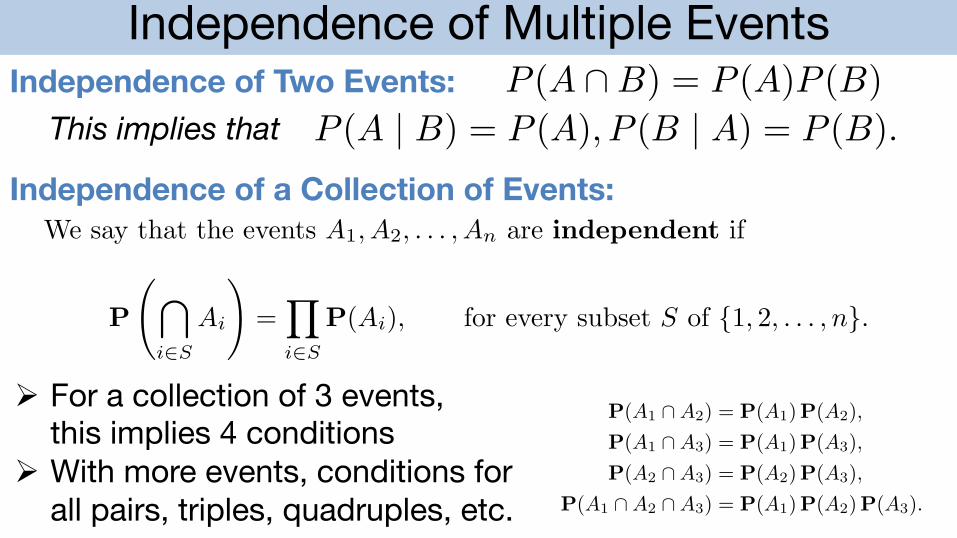
Independence of Multiple EventsIndependence of Two Events: P (A \B) = P (A)P (B)
P (A | B) = P (A), P (B | A) = P (B).This implies thatIndependence of a Collection of Events:
36 Sample Space and Probability Chap. 1
Definition of Independence of Several Events
We say that the events A1, A2, . . . , An are independent if
P
!"
i∈S
Ai
#=
$
i∈S
P(Ai), for every subset S of 1 , 2 , . . . , n.
If we have a collection of three events, A1, A2, and A3, independenceamounts to satisfying the four conditions
P(A1 ∩ A2) = P(A1)P(A2),P(A1 ∩ A3) = P(A1)P(A3),P(A2 ∩ A3) = P(A2)P(A3),
P(A1 ∩ A2 ∩ A3) = P(A1)P(A2)P(A3).
The first three conditions simply assert that any two events are independent,a property known as pairwise independence. But the fourth condition isalso important and does not follow from the first three. Conversely, the fourthcondition does not imply the first three; see the two examples that follow.
Example 1.20. Pairwise independence does not imply independence.Consider two independent fair coin tosses, and the following events:
H1 = 1st toss is a head,
H2 = 2nd toss is a head,
D = the two tosses have different results.
The events H1 and H2 are independent, by definition. To see that H1 and D areindependent, we note that
P(D |H1) =P(H1 ∩ D)
P(H1)=
1/4
1/2=
12
= P(D).
Similarly, H2 and D are independent. On the other hand, we have
P(H1 ∩ H2 ∩ D) = 0 = 12· 12· 12
= P(H1)P(H2)P(D),
and these three events are not independent.
Example 1.21. The equality P(A1 ∩ A2 ∩ A3) = P(A1)P(A2)P(A3) is notenough for independence. Consider two independent rolls of a fair die, and
Ø For a collection of 3 events,this implies 4 conditions
Ø With more events, conditions for all pairs, triples, quadruples, etc.
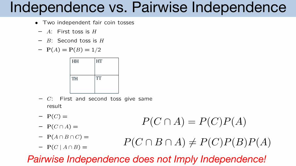
Independence vs. Pairwise Independence
Conditioning may aect independence Independence of a collection of events
• Two unfair coins, A and B: • Intuitive definition:P(H | coin A) = 0.9, P(H | coin B) = 0.1 Information on some of the events tellschoose either coin with equal probability
us nothing about probabilities related to0.9 the remaining events
0.10.9 – E.g.:Coin A
P( ( c ) | c ) = P( ( c0.9 A1 A2 A3 A5 A6 A1 A2 A3))
0.5 0.10.1
• Mathematical definition:0.1 Events A1, A2, . . . , An
0.50.1
0.9are called independent if:
Coin B 0.1
0.9P(AiAj· · ·Aq) = P(Ai)P(Aj) · · ·P(Aq)
0.9 for any distinct indices i, j, . . . , q,(chosen from 1, . . . , n )
• Once we know it is coin A, are tosses
independent?
• If we do not know which coin it is, aretosses independent?
– Compare:P(toss 11 = H)P(toss 11 = H | first 10 tosses are heads)
Independence vs. pairwise The king’s sibling
independence• The king comes from a family of two
• Two independent fair coin tosses children. What is the probability that
– A: First toss is H his sibling is female?
– B: Second toss is H
– P(A) = P(B) = 1/2
HH HT
TH TT
– C: First and second toss give sameresult
– P(C) =
– P(C A) =
– P(A B C) =
– P(C | A B) =
• Pairwise independence does not
imply independence
2
P (C \A) = P (C)P (A)
Pairwise Independence does not Imply Independence!P (C \B \A) 6= P (C)P (B)P (A)
CS145: Lecture 4 OutlineØ Independence and Conditional IndependenceØBayes’ Rule and ClassificationØDiscrete random variables
Boxes and Balls
1.5
Example 1.
Problem.
Solution.
Section 1.5. Bayes' Rule 47
Bayes' Rule The rules of conditional probability, described in the last section, combine to give a general formula for updating probabilities called Bayes' rule. Before stating the rule in general, here is an example to illustrate the basic setup.
Which box? Suppose there are three similar boxes. Box i contains i white balls and one black ball, i = 1,2,3, as shown in the following diagram.
loelloil Box 1 Box 2
1001 Box 3
Suppose I mix up the boxes and then pick one at random. Then I pick a ball at random from the box and show you the ball. I offer you a prize if you can guess correctly what box it came from.
Which box would you guess if the ball drawn is white and what is your chance of guessing right?
An intuitively reasonable guess is Box 3, because the most likely explanation of how a white ball was drawn is that it came from a box with a large proportion of whites. To confirm this, here is a calculation of
P( '1 h') P(Box i and white) Box t w He = ( ) P white
(i = 1,2,3)
These are the chances that you would be right if you guessed Box i, given that the ball drawn is white. The following diagram shows the probabilistic assumptions:
Pick Box Pick Ball
bJ 1 2
1/3 1/2
1 3 loil 2/3
1/3
1/3 3/4
o. 1/4
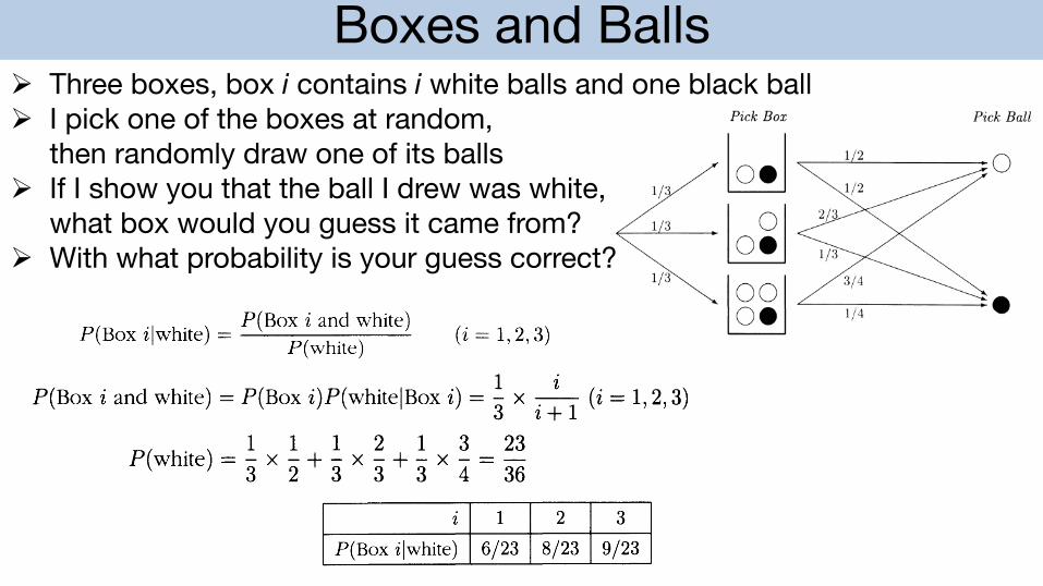
Ø Three boxes, box i contains i white balls and one black ballØ I pick one of the boxes at random,
then randomly draw one of its ballsØ If I show you that the ball I drew was white,
what box would you guess it came from?Ø With what probability is your guess correct?
1.5
Example 1.
Problem.
Solution.
Section 1.5. Bayes' Rule 47
Bayes' Rule The rules of conditional probability, described in the last section, combine to give a general formula for updating probabilities called Bayes' rule. Before stating the rule in general, here is an example to illustrate the basic setup.
Which box? Suppose there are three similar boxes. Box i contains i white balls and one black ball, i = 1,2,3, as shown in the following diagram.
loelloil Box 1 Box 2
1001 Box 3
Suppose I mix up the boxes and then pick one at random. Then I pick a ball at random from the box and show you the ball. I offer you a prize if you can guess correctly what box it came from.
Which box would you guess if the ball drawn is white and what is your chance of guessing right?
An intuitively reasonable guess is Box 3, because the most likely explanation of how a white ball was drawn is that it came from a box with a large proportion of whites. To confirm this, here is a calculation of
P( '1 h') P(Box i and white) Box t w He = ( ) P white
(i = 1,2,3)
These are the chances that you would be right if you guessed Box i, given that the ball drawn is white. The following diagram shows the probabilistic assumptions:
Pick Box Pick Ball
bJ 1 2
1/3 1/2
1 3 loil 2/3
1/3
1/3 3/4
o. 1/4
48 Chapter 1. Introduction
From the diagram, the numerator in (*) is
1 i P(Box i and white) = P(Box i)P(whiteIBox i) = 3" x i + 1 (i = 1,2,3)
By the addition rule, the denominator in (*) is the sum of these terms over i = 1, 2, 3:
1 1 1 2 1 3 23 P(white) = 3" x 2" + 3" x 3" + 3" x 4 = 36 and
1 i 12 ,; 3 x HI • P(Box ilwhite) = 23 = - X --36 23 i + 1
(i=1,2,3)
Substituting for i/(i + 1) for i = 1,2,3 gives the following numerical results:
i 1 2 3
P(Box ilwhite) 6/23 8/23 9/23
This confirms the intuitive idea that Box 3 is the most likely explanation of a white ball. Given a white ball, the chance that you would be right if you guessed this box would be 9/23 39.13%.
Suppose, more generally, that events B l , ... , Bn represent n mutually exclusive possible results of the first stage of some procedure. Which one of these results has occurred is assumed unknown. Rather, the result A of some second stage has been observed, whose chances depend on which of the Bi'S has occurred. In the previous example A was the event that a white ball was drawn and Bi the event that it came from a box with i white balls. The general problem is to calculate the probabilities of the events Bi given occurrence of A (called posterior probabilities), in terms of
co the unconditional probabilities P(Bi ) (called prior probabilities);
(ii) the conditional probabilities P(AIBi) (called likelihoods).
Here is the general calculation:
(multiplication rule)
where, by the rule of average conditional probabilities, the denominator is
P(A) = P(AIBdP(Bd + ... + P(AIBn)P(Bn)
which is the sum over i = 1 to n of the expression P(AIBi)P(Bi ) in the numerator. The result of this calculation is called Bayes' rule.
Total Probability and Bayes’ Theorem
Models based on conditional Multiplication rule
probabilities
P(A B C) = P(A) P(B A) P(C A B)• Event A: Airplane is flying above
· | · |
Event B: Something registers on radarscreen
A
U
B P(C | A
U
B)P(B | A)=0.99 A
U
B
U
C
P(B | A)cP(B | A)=0.01
P(A)=0.05A
cP(B | A)cA
U
B
U
CP(A)
A
U
cBcP(A )=0.95cA
U
cB
U
CcP(B | A )=0.10
c cP(B | A )=0.90 cP(A )
cA
P(A B) =
P(B) =
P(A | B) =
Total probability theorem Bayes’ rule
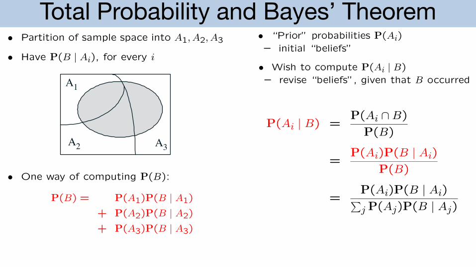
• Divide and conquer • “Prior” probabilities P(Ai)– initial “beliefs”
• Partition of sample space into A1, A2, A3• We know P(B | Ai) for each i
• Have P(B | Ai), for every i• Wish to compute P(Ai | B)
A– revise “beliefs”, given that B occurred
1
B
A1
B
A A2 3
• One way of computing AP( AB): 2 3
P(B) = P(A1)P(B | A1)
+ P(A2)P(B | A2)P(+ ( ) ( | ) Ai B)P A3 P B A3 P(Ai | B) =
P(B)
P(Ai)P(B=
| Ai)
P(B)
P(A )P(B A )= i | i
j P(Aj)P(B | Aj)
Multiplication rule
P(A ∩B ∩ C) = P(A)P(B | A)P(C | A ∩B)
2
Models based on conditional Multiplication rule
probabilities
P(A B C) = P(A) P(B A) P(C A B)• Event A: Airplane is flying above
· | · |
Event B: Something registers on radarscreen
A
U
B P(C | A
U
B)P(B | A)=0.99 A
U
B
U
C
P(B | A)cP(B | A)=0.01
P(A)=0.05A
cP(B | A)cA
U
B
U
CP(A)
A
U
cBcP(A )=0.95cA
U
cB
U
CcP(B | A )=0.10
c cP(B | A )=0.90 cP(A )
cA
P(A B) =
P(B) =
P(A | B) =
Total probability theorem Bayes’ rule
• Divide and conquer • “Prior” probabilities P(Ai)– initial “beliefs”
• Partition of sample space into A1, A2, A3• We know P(B | Ai) for each i
• Have P(B | Ai), for every i• Wish to compute P(Ai | B)
A– revise “beliefs”, given that B occurred
1
B
A1
B
A A2 3
• One way of computing AP( AB): 2 3
P(B) = P(A1)P(B | A1)
+ P(A2)P(B | A2)P(+ ( ) ( | ) Ai B)P A3 P B A3 P(Ai | B) =
P(B)
P(Ai)P(B=
| Ai)
P(B)
P(A )P(B A )= i | i
j P(Aj)P(B | Aj)
Multiplication rule
P(A ∩B ∩ C) = P(A)P(B | A)P(C | A ∩B)
2
Classification Problems
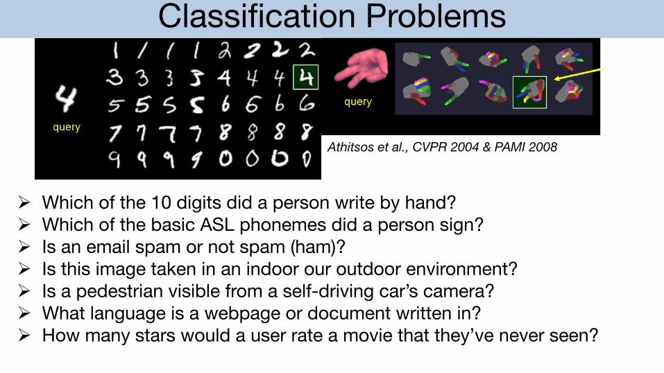
Athitsos et al., CVPR 2004 & PAMI 2008
Ø Which of the 10 digits did a person write by hand?Ø Which of the basic ASL phonemes did a person sign?Ø Is an email spam or not spam (ham)?Ø Is this image taken in an indoor our outdoor environment?Ø Is a pedestrian visible from a self-driving car’s camera?Ø What language is a webpage or document written in?Ø How many stars would a user rate a movie that they’ve never seen?
Models Based on Conditional ProbabilitiesModels based on conditional Multiplication rule
probabilities
P(A B C) = P(A) P(B A) P(C A B)• Event A: Airplane is flying above
· | · |
Event B: Something registers on radarscreen
A
U
B P(C | A
U
B)P(B | A)=0.99 A
U
B
U
C
P(B | A)cP(B | A)=0.01
P(A)=0.05A
cP(B | A)cA
U
B
U
CP(A)
A
U
cBcP(A )=0.95cA
U
cB
U
CcP(B | A )=0.10
c cP(B | A )=0.90 cP(A )
cA
P(A B) =
P(B) =
P(A | B) =
Total probability theorem Bayes’ rule
• Divide and conquer • “Prior” probabilities P(Ai)– initial “beliefs”
• Partition of sample space into A1, A2, A3• We know P(B | Ai) for each i
• Have P(B | Ai), for every i• Wish to compute P(Ai | B)
A– revise “beliefs”, given that B occurred
1
B
A1
B
A A2 3
• One way of computing AP( AB): 2 3
P(B) = P(A1)P(B | A1)
+ P(A2)P(B | A2)P(+ ( ) ( | ) Ai B)P A3 P B A3 P(Ai | B) =
P(B)
P(Ai)P(B=
| Ai)
P(B)
P(A )P(B A )= i | i
j P(Aj)P(B | Aj)
Multiplication rule
P(A ∩B ∩ C) = P(A)P(B | A)P(C | A ∩B)
2
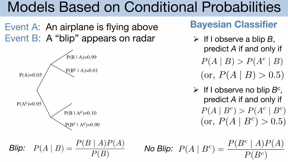
Event A: An airplane is flying aboveEvent B: A “blip” appears on radar
P (A | B) =P (B | A)P (A)
P (B)P (A | Bc) =
P (Bc | A)P (A)
P (Bc)Blip: No Blip:
Bayesian ClassifierØ If I observe a blip B,
predict A if and only ifP (A | B) > P (Ac | B)
Ø If I observe no blip Bc, predict A if and only ifP (A | Bc) > P (Ac | Bc)
(or, P (A | B) > 0.5)
(or, P (A | Bc) > 0.5)
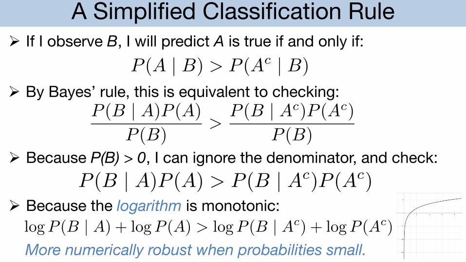
A Simplified Classification RuleØ If I observe B, I will predict A is true if and only if:
P (A | B) > P (Ac | B)
P (B | A)P (A)
P (B)>
P (B | Ac)P (Ac)
P (B)
Ø By Bayes’ rule, this is equivalent to checking:
Ø Because P(B) > 0, I can ignore the denominator, and check:P (B | A)P (A) > P (B | Ac)P (Ac)
Ø Because the logarithm is monotonic:logP (B | A) + logP (A) > logP (B | Ac) + logP (Ac)
More numerically robust when probabilities small.
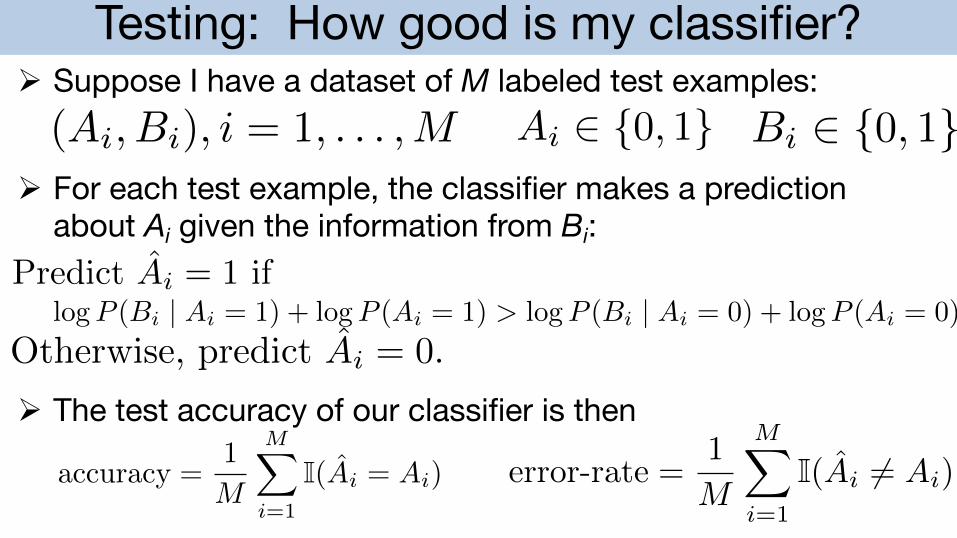
Testing: How good is my classifier?Ø Suppose I have a dataset of M labeled test examples:(Ai, Bi), i = 1, . . . ,M Ai 2 0, 1 Bi 2 0, 1
Ø For each test example, the classifier makes a predictionabout Ai given the information from Bi:
logP (Bi | Ai = 1) + logP (Ai = 1) > logP (Bi | Ai = 0) + logP (Ai = 0)Predict Ai = 1 if
Otherwise, predict Ai = 0.
Ø The test accuracy of our classifier is then
accuracy =1
M
MX
i=1
I(Ai = Ai) error-rate =1
M
MX
i=1
I(Ai 6= Ai)
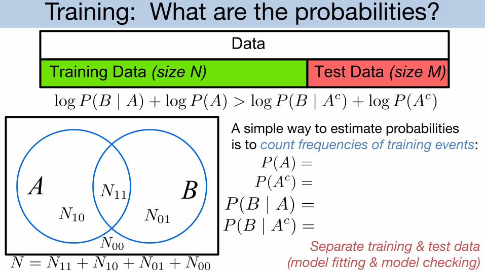
Training: What are the probabilities?Data
Training Data (size N) Test Data (size M)
logP (B | A) + logP (A) > logP (B | Ac) + logP (Ac)
A B
N = N11 +N10 +N01 +N00
N11
N10 N01
N00
A simple way to estimate probabilities is to count frequencies of training events:
P (A) =P (Ac) =
P (B | Ac) =P (B | A) =
Separate training & test data (model fitting & model checking)
CS145: Lecture 4 OutlineØ Independence and Conditional IndependenceØBayes’ Rule and ClassificationØDiscrete random variables
Discrete Random Variables
6 Sample Space and Probability Chap. 1
of every Sn, and xn ∈ ∩nScn. This shows that (∪nSn)c ⊂ ∩nSc
n. The converseinclusion is established by reversing the above argument, and the first law follows.The argument for the second law is similar.
1.2 PROBABILISTIC MODELS
A probabilistic model is a mathematical description of an uncertain situation.It must be in accordance with a fundamental framework that we discuss in thissection. Its two main ingredients are listed below and are visualized in Fig. 1.2.
Elements of a Probabilistic Model
• The sample space Ω, which is the set of all possible outcomes of anexperiment.
• The probability law, which assigns to a set A of possible outcomes(also called an event) a nonnegative number P(A) (called the proba-bility of A) that encodes our knowledge or belief about the collective“likelihood” of the elements of A. The probability law must satisfycertain properties to be introduced shortly.
Experiment
Sample Space 1(Set of Outcomes)
Event A
Event B
A B Events
P(A)
P(B)
ProbabilityLaw
Figure 1.2: The main ingredients of a probabilistic model.
Sample Spaces and Events
Every probabilistic model involves an underlying process, called the experi-ment, that will produce exactly one out of several possible outcomes. The setof all possible outcomes is called the sample space of the experiment, and isdenoted by Ω. A subset of the sample space, that is, a collection of possible
X : ! R x = X(!) 2 R for ! 2
2 Discrete Random Variables Chap. 2
2.1 BASIC CONCEPTS
In many probabilistic models, the outcomes are of a numerical nature, e.g., ifthey correspond to instrument readings or stock prices. In other experiments,the outcomes are not numerical, but they may be associated with some numericalvalues of interest. For example, if the experiment is the selection of students froma given population, we may wish to consider their grade point average. Whendealing with such numerical values, it is often useful to assign probabilities tothem. This is done through the notion of a random variable, the focus of thepresent chapter.
Given an experiment and the corresponding set of possible outcomes (thesample space), a random variable associates a particular number with each out-come; see Fig. 2.1. We refer to this number as the numerical value or theexperimental value of the random variable. Mathematically, a random vari-able is a real-valued function of the experimental outcome.
11 2
2
3
3
4
4
Real Number Line1 2 3 4
(a)
(b)
Sample Space1 x
Random Variable X
Real Number Line
Random Variable:X = Maximum Roll
Sample Space:Pairs of Rolls
Figure 2.1: (a) Visualization of a random variable. It is a function that assignsa numerical value to each possible outcome of the experiment. (b) An exampleof a random variable. The experiment consists of two rolls of a 4-sided die, andthe random variable is the maximum of the two rolls. If the outcome of theexperiment is (4, 2), the experimental value of this random variable is 4.
Here are some examples of random variables:
(a) In an experiment involving a sequence of 5 tosses of a coin, the number ofheads in the sequence is a random variable. However, the 5-long sequence
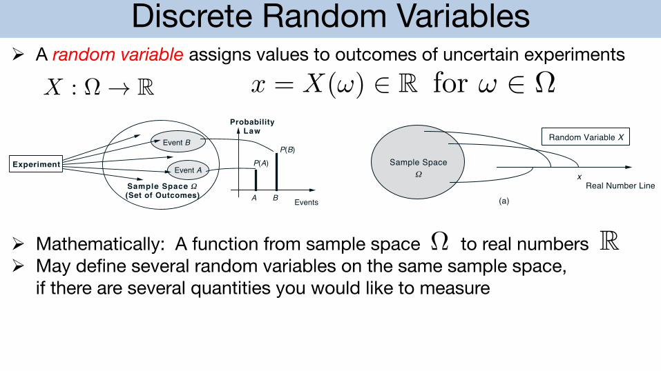
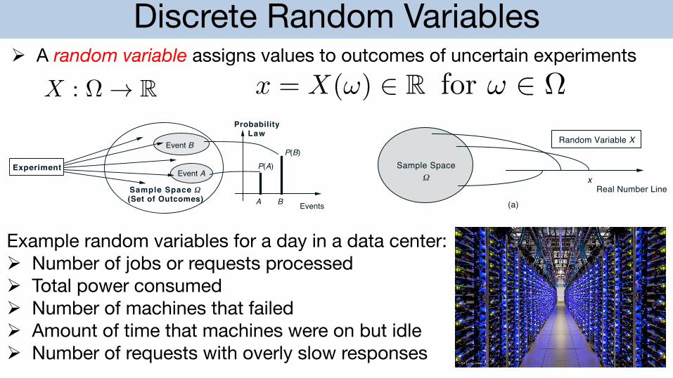
Ø A random variable assigns values to outcomes of uncertain experiments
Ø Mathematically: A function from sample space to real numbersØ May define several random variables on the same sample space,
if there are several quantities you would like to measure
R
Discrete Random Variables
6 Sample Space and Probability Chap. 1
of every Sn, and xn ∈ ∩nScn. This shows that (∪nSn)c ⊂ ∩nSc
n. The converseinclusion is established by reversing the above argument, and the first law follows.The argument for the second law is similar.
1.2 PROBABILISTIC MODELS
A probabilistic model is a mathematical description of an uncertain situation.It must be in accordance with a fundamental framework that we discuss in thissection. Its two main ingredients are listed below and are visualized in Fig. 1.2.
Elements of a Probabilistic Model
• The sample space Ω, which is the set of all possible outcomes of anexperiment.
• The probability law, which assigns to a set A of possible outcomes(also called an event) a nonnegative number P(A) (called the proba-bility of A) that encodes our knowledge or belief about the collective“likelihood” of the elements of A. The probability law must satisfycertain properties to be introduced shortly.
Experiment
Sample Space 1(Set of Outcomes)
Event A
Event B
A B Events
P(A)
P(B)
ProbabilityLaw
Figure 1.2: The main ingredients of a probabilistic model.
Sample Spaces and Events
Every probabilistic model involves an underlying process, called the experi-ment, that will produce exactly one out of several possible outcomes. The setof all possible outcomes is called the sample space of the experiment, and isdenoted by Ω. A subset of the sample space, that is, a collection of possible
X : ! R x = X(!) 2 R for ! 2
2 Discrete Random Variables Chap. 2
2.1 BASIC CONCEPTS
In many probabilistic models, the outcomes are of a numerical nature, e.g., ifthey correspond to instrument readings or stock prices. In other experiments,the outcomes are not numerical, but they may be associated with some numericalvalues of interest. For example, if the experiment is the selection of students froma given population, we may wish to consider their grade point average. Whendealing with such numerical values, it is often useful to assign probabilities tothem. This is done through the notion of a random variable, the focus of thepresent chapter.
Given an experiment and the corresponding set of possible outcomes (thesample space), a random variable associates a particular number with each out-come; see Fig. 2.1. We refer to this number as the numerical value or theexperimental value of the random variable. Mathematically, a random vari-able is a real-valued function of the experimental outcome.
11 2
2
3
3
4
4
Real Number Line1 2 3 4
(a)
(b)
Sample Space1 x
Random Variable X
Real Number Line
Random Variable:X = Maximum Roll
Sample Space:Pairs of Rolls
Figure 2.1: (a) Visualization of a random variable. It is a function that assignsa numerical value to each possible outcome of the experiment. (b) An exampleof a random variable. The experiment consists of two rolls of a 4-sided die, andthe random variable is the maximum of the two rolls. If the outcome of theexperiment is (4, 2), the experimental value of this random variable is 4.
Here are some examples of random variables:
(a) In an experiment involving a sequence of 5 tosses of a coin, the number ofheads in the sequence is a random variable. However, the 5-long sequence
Ø A random variable assigns values to outcomes of uncertain experiments
Example random variables for a day in a data center:Ø Number of jobs or requests processedØ Total power consumedØ Number of machines that failedØ Amount of time that machines were on but idleØ Number of requests with overly slow responses
Discrete Random Variables
6 Sample Space and Probability Chap. 1
of every Sn, and xn ∈ ∩nScn. This shows that (∪nSn)c ⊂ ∩nSc
n. The converseinclusion is established by reversing the above argument, and the first law follows.The argument for the second law is similar.
1.2 PROBABILISTIC MODELS
A probabilistic model is a mathematical description of an uncertain situation.It must be in accordance with a fundamental framework that we discuss in thissection. Its two main ingredients are listed below and are visualized in Fig. 1.2.
Elements of a Probabilistic Model
• The sample space Ω, which is the set of all possible outcomes of anexperiment.
• The probability law, which assigns to a set A of possible outcomes(also called an event) a nonnegative number P(A) (called the proba-bility of A) that encodes our knowledge or belief about the collective“likelihood” of the elements of A. The probability law must satisfycertain properties to be introduced shortly.
Experiment
Sample Space 1(Set of Outcomes)
Event A
Event B
A B Events
P(A)
P(B)
ProbabilityLaw
Figure 1.2: The main ingredients of a probabilistic model.
Sample Spaces and Events
Every probabilistic model involves an underlying process, called the experi-ment, that will produce exactly one out of several possible outcomes. The setof all possible outcomes is called the sample space of the experiment, and isdenoted by Ω. A subset of the sample space, that is, a collection of possible
X : ! R x = X(!) 2 R for ! 2
2 Discrete Random Variables Chap. 2
2.1 BASIC CONCEPTS
In many probabilistic models, the outcomes are of a numerical nature, e.g., ifthey correspond to instrument readings or stock prices. In other experiments,the outcomes are not numerical, but they may be associated with some numericalvalues of interest. For example, if the experiment is the selection of students froma given population, we may wish to consider their grade point average. Whendealing with such numerical values, it is often useful to assign probabilities tothem. This is done through the notion of a random variable, the focus of thepresent chapter.
Given an experiment and the corresponding set of possible outcomes (thesample space), a random variable associates a particular number with each out-come; see Fig. 2.1. We refer to this number as the numerical value or theexperimental value of the random variable. Mathematically, a random vari-able is a real-valued function of the experimental outcome.
11 2
2
3
3
4
4
Real Number Line1 2 3 4
(a)
(b)
Sample Space1 x
Random Variable X
Real Number Line
Random Variable:X = Maximum Roll
Sample Space:Pairs of Rolls
Figure 2.1: (a) Visualization of a random variable. It is a function that assignsa numerical value to each possible outcome of the experiment. (b) An exampleof a random variable. The experiment consists of two rolls of a 4-sided die, andthe random variable is the maximum of the two rolls. If the outcome of theexperiment is (4, 2), the experimental value of this random variable is 4.
Here are some examples of random variables:
(a) In an experiment involving a sequence of 5 tosses of a coin, the number ofheads in the sequence is a random variable. However, the 5-long sequence
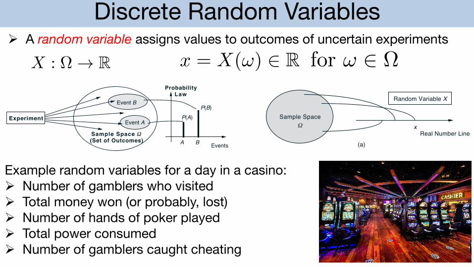
Ø A random variable assigns values to outcomes of uncertain experiments
Example random variables for a day in a casino:Ø Number of gamblers who visitedØ Total money won (or probably, lost)Ø Number of hands of poker playedØ Total power consumedØ Number of gamblers caught cheating
Discrete Random Variables
6 Sample Space and Probability Chap. 1
of every Sn, and xn ∈ ∩nScn. This shows that (∪nSn)c ⊂ ∩nSc
n. The converseinclusion is established by reversing the above argument, and the first law follows.The argument for the second law is similar.
1.2 PROBABILISTIC MODELS
A probabilistic model is a mathematical description of an uncertain situation.It must be in accordance with a fundamental framework that we discuss in thissection. Its two main ingredients are listed below and are visualized in Fig. 1.2.
Elements of a Probabilistic Model
• The sample space Ω, which is the set of all possible outcomes of anexperiment.
• The probability law, which assigns to a set A of possible outcomes(also called an event) a nonnegative number P(A) (called the proba-bility of A) that encodes our knowledge or belief about the collective“likelihood” of the elements of A. The probability law must satisfycertain properties to be introduced shortly.
Experiment
Sample Space 1(Set of Outcomes)
Event A
Event B
A B Events
P(A)
P(B)
ProbabilityLaw
Figure 1.2: The main ingredients of a probabilistic model.
Sample Spaces and Events
Every probabilistic model involves an underlying process, called the experi-ment, that will produce exactly one out of several possible outcomes. The setof all possible outcomes is called the sample space of the experiment, and isdenoted by Ω. A subset of the sample space, that is, a collection of possible
X : ! R x = X(!) 2 R for ! 2
2 Discrete Random Variables Chap. 2
2.1 BASIC CONCEPTS
In many probabilistic models, the outcomes are of a numerical nature, e.g., ifthey correspond to instrument readings or stock prices. In other experiments,the outcomes are not numerical, but they may be associated with some numericalvalues of interest. For example, if the experiment is the selection of students froma given population, we may wish to consider their grade point average. Whendealing with such numerical values, it is often useful to assign probabilities tothem. This is done through the notion of a random variable, the focus of thepresent chapter.
Given an experiment and the corresponding set of possible outcomes (thesample space), a random variable associates a particular number with each out-come; see Fig. 2.1. We refer to this number as the numerical value or theexperimental value of the random variable. Mathematically, a random vari-able is a real-valued function of the experimental outcome.
11 2
2
3
3
4
4
Real Number Line1 2 3 4
(a)
(b)
Sample Space1 x
Random Variable X
Real Number Line
Random Variable:X = Maximum Roll
Sample Space:Pairs of Rolls
Figure 2.1: (a) Visualization of a random variable. It is a function that assignsa numerical value to each possible outcome of the experiment. (b) An exampleof a random variable. The experiment consists of two rolls of a 4-sided die, andthe random variable is the maximum of the two rolls. If the outcome of theexperiment is (4, 2), the experimental value of this random variable is 4.
Here are some examples of random variables:
(a) In an experiment involving a sequence of 5 tosses of a coin, the number ofheads in the sequence is a random variable. However, the 5-long sequence
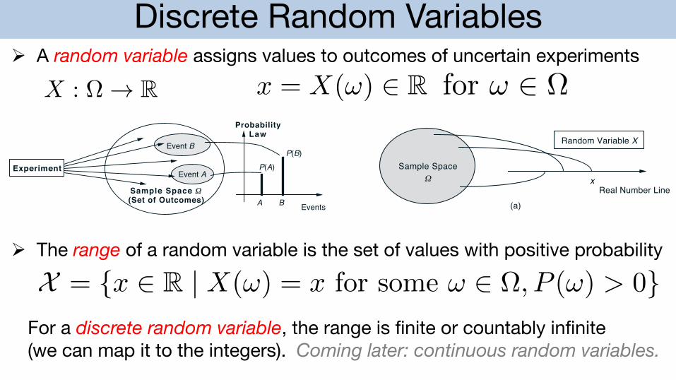
Ø A random variable assigns values to outcomes of uncertain experiments
Ø The range of a random variable is the set of values with positive probability
X = x 2 R | X(!) = x for some ! 2 , P (!) > 0For a discrete random variable, the range is finite or countably infinite (we can map it to the integers). Coming later: continuous random variables.
Discrete Random Variables
6 Sample Space and Probability Chap. 1
of every Sn, and xn ∈ ∩nScn. This shows that (∪nSn)c ⊂ ∩nSc
n. The converseinclusion is established by reversing the above argument, and the first law follows.The argument for the second law is similar.
1.2 PROBABILISTIC MODELS
A probabilistic model is a mathematical description of an uncertain situation.It must be in accordance with a fundamental framework that we discuss in thissection. Its two main ingredients are listed below and are visualized in Fig. 1.2.
Elements of a Probabilistic Model
• The sample space Ω, which is the set of all possible outcomes of anexperiment.
• The probability law, which assigns to a set A of possible outcomes(also called an event) a nonnegative number P(A) (called the proba-bility of A) that encodes our knowledge or belief about the collective“likelihood” of the elements of A. The probability law must satisfycertain properties to be introduced shortly.
Experiment
Sample Space 1(Set of Outcomes)
Event A
Event B
A B Events
P(A)
P(B)
ProbabilityLaw
Figure 1.2: The main ingredients of a probabilistic model.
Sample Spaces and Events
Every probabilistic model involves an underlying process, called the experi-ment, that will produce exactly one out of several possible outcomes. The setof all possible outcomes is called the sample space of the experiment, and isdenoted by Ω. A subset of the sample space, that is, a collection of possible
X : ! R x = X(!) 2 R for ! 2
2 Discrete Random Variables Chap. 2
2.1 BASIC CONCEPTS
In many probabilistic models, the outcomes are of a numerical nature, e.g., ifthey correspond to instrument readings or stock prices. In other experiments,the outcomes are not numerical, but they may be associated with some numericalvalues of interest. For example, if the experiment is the selection of students froma given population, we may wish to consider their grade point average. Whendealing with such numerical values, it is often useful to assign probabilities tothem. This is done through the notion of a random variable, the focus of thepresent chapter.
Given an experiment and the corresponding set of possible outcomes (thesample space), a random variable associates a particular number with each out-come; see Fig. 2.1. We refer to this number as the numerical value or theexperimental value of the random variable. Mathematically, a random vari-able is a real-valued function of the experimental outcome.
11 2
2
3
3
4
4
Real Number Line1 2 3 4
(a)
(b)
Sample Space1 x
Random Variable X
Real Number Line
Random Variable:X = Maximum Roll
Sample Space:Pairs of Rolls
Figure 2.1: (a) Visualization of a random variable. It is a function that assignsa numerical value to each possible outcome of the experiment. (b) An exampleof a random variable. The experiment consists of two rolls of a 4-sided die, andthe random variable is the maximum of the two rolls. If the outcome of theexperiment is (4, 2), the experimental value of this random variable is 4.
Here are some examples of random variables:
(a) In an experiment involving a sequence of 5 tosses of a coin, the number ofheads in the sequence is a random variable. However, the 5-long sequence
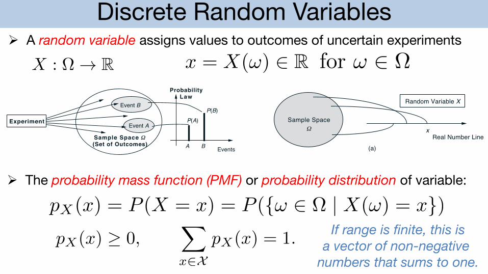
Ø A random variable assigns values to outcomes of uncertain experiments
Ø The probability mass function (PMF) or probability distribution of variable:
pX(x) = P (X = x) = P (! 2 | X(!) = x)pX(x) 0,
X
x2XpX(x) = 1.
If range is finite, this isa vector of non-negative
numbers that sums to one.