CS145: INTRODUCTION TO DATA MINING

Instructor: Yizhou Sunyzsun@cs.ucla.edu

October 24, 2017

08: Classification Evaluation and Practical Issues

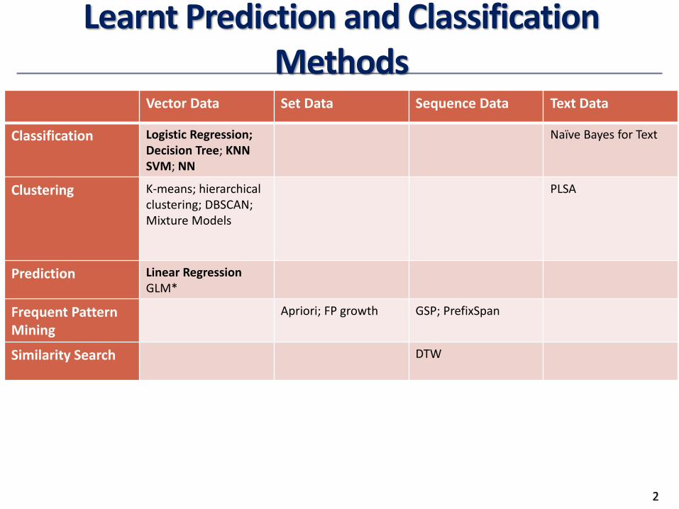
Learnt Prediction and Classification Methods

2

Vector Data Set Data Sequence Data Text Data

Classification Logistic Regression; Decision Tree; KNNSVM; NN

Naïve Bayes for Text

Clustering K-means; hierarchicalclustering; DBSCAN; Mixture Models

PLSA

Prediction Linear RegressionGLM*

Frequent Pattern Mining

Apriori; FP growth GSP; PrefixSpan

Similarity Search DTW

Evaluation and Other Practical Issues

•Model Evaluation and Selection

•Other issues

•Summary

3

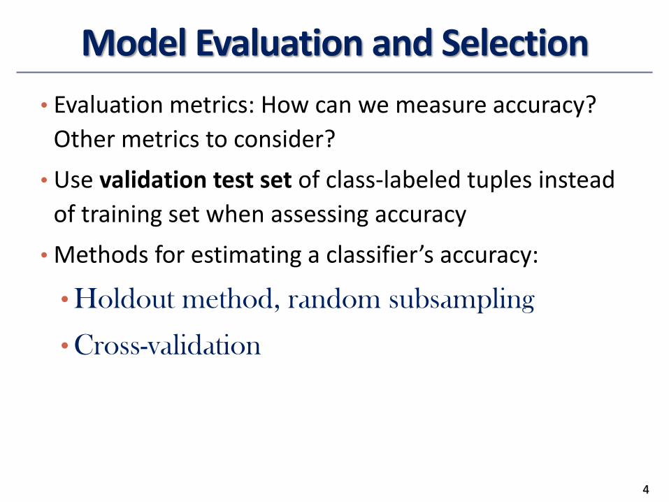
Model Evaluation and Selection

• Evaluation metrics: How can we measure accuracy?

Other metrics to consider?

• Use validation test set of class-labeled tuples instead

of training set when assessing accuracy

• Methods for estimating a classifier’s accuracy:

•Holdout method, random subsampling

•Cross-validation

4

Evaluating Classifier Accuracy:Holdout & Cross-Validation Methods

• Holdout method• Given data is randomly partitioned into two independent sets

• Training set (e.g., 2/3) for model construction• Test set (e.g., 1/3) for accuracy estimation

• Random sampling: a variation of holdout

• Repeat holdout k times, accuracy = avg. of the accuracies obtained

• Cross-validation (k-fold, where k = 10 is most popular)• Randomly partition the data into k mutually exclusive subsets, each

approximately equal size• At i-th iteration, use Di as test set and others as training set• Leave-one-out: k folds where k = # of tuples, for small sized data• *Stratified cross-validation*: folds are stratified so that class dist. in

each fold is approx. the same as that in the whole data

5

Classifier Evaluation Metrics: Confusion Matrix

Actual class\Predicted class

buy_computer = yes

buy_computer = no

Total

buy_computer = yes 6954 46 7000

buy_computer = no 412 2588 3000

Total 7366 2634 10000

• Given m classes, an entry, CMi,j in a confusion matrix indicates # of tuples in class i that were labeled by the classifier as class j

• May have extra rows/columns to provide totals

Confusion Matrix:

Actual class\Predicted class C1 ¬ C1

C1 True Positives (TP) False Negatives (FN)

¬ C1 False Positives (FP) True Negatives (TN)

Example of Confusion Matrix:

6

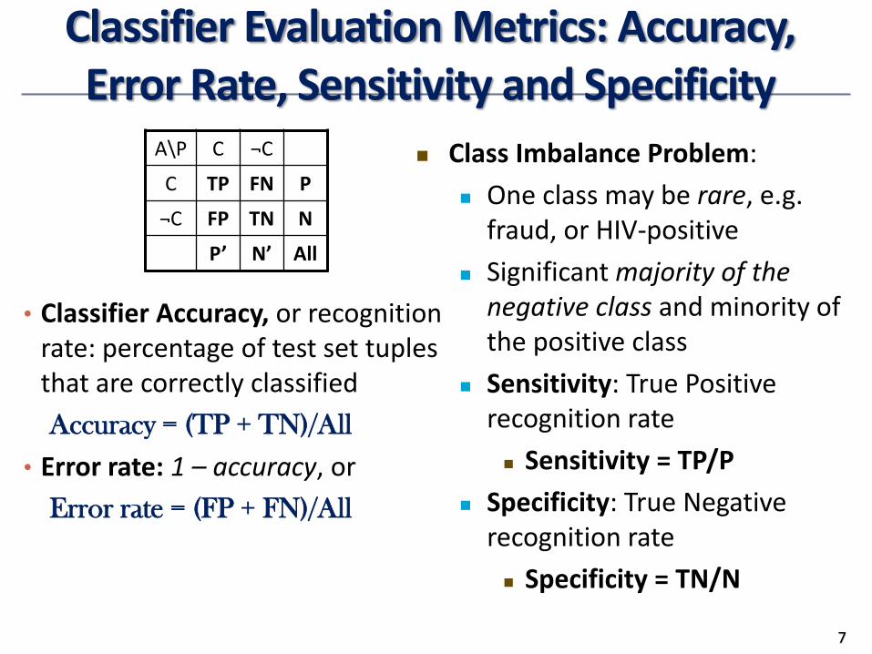
Classifier Evaluation Metrics: Accuracy, Error Rate, Sensitivity and Specificity

• Classifier Accuracy, or recognition rate: percentage of test set tuples that are correctly classified

Accuracy = (TP + TN)/All

• Error rate: 1 – accuracy, or

Error rate = (FP + FN)/All

7

Class Imbalance Problem:

One class may be rare, e.g. fraud, or HIV-positive

Significant majority of the negative class and minority of the positive class

Sensitivity: True Positive recognition rate

Sensitivity = TP/P

Specificity: True Negative recognition rate

Specificity = TN/N

A\P C ¬C

C TP FN P

¬C FP TN N

P’ N’ All

Classifier Evaluation Metrics: Precision and Recall, and F-measures

• Precision: exactness – what % of tuples that the classifier labeled as positive are actually positive

• Recall: completeness – what % of positive tuples did the classifier label as positive?

• Perfect score is 1.0• Inverse relationship between precision & recall• F measure (F1 or F-score): harmonic mean of precision and

recall,

• Fß: weighted measure of precision and recall• assigns ß times as much weight to recall as to precision

8

Classifier Evaluation Metrics: Example

• Precision = 90/230 = 39.13% Recall = 90/300 = 30.00%

Actual Class\Predicted class cancer = yes cancer = no Total Recognition(%)

cancer = yes 90 210 300 30.00 (sensitivity)

cancer = no 140 9560 9700 98.56 (specificity)

Total 230 9770 10000 96.50 (accuracy)

9

10

Classifier Evaluation Metrics: ROC Curves

• ROC (Receiver Operating Characteristics) curves: for visual comparison of classification models

• Originated from signal detection theory• Shows the trade-off between the true

positive rate and the false positive rate• The area under the ROC curve is a

measure of the accuracy of the model• Rank the test tuples in decreasing

order: the one that is most likely to belong to the positive class appears at the top of the list

• Area under the curve: the closer to the diagonal line (i.e., the closer the area is to 0.5), the less accurate is the model

Vertical axis represents the true positive rate

Horizontal axis rep. the false positive rate

The plot also shows a diagonal line

A model with perfect accuracy will have an area of 1.0

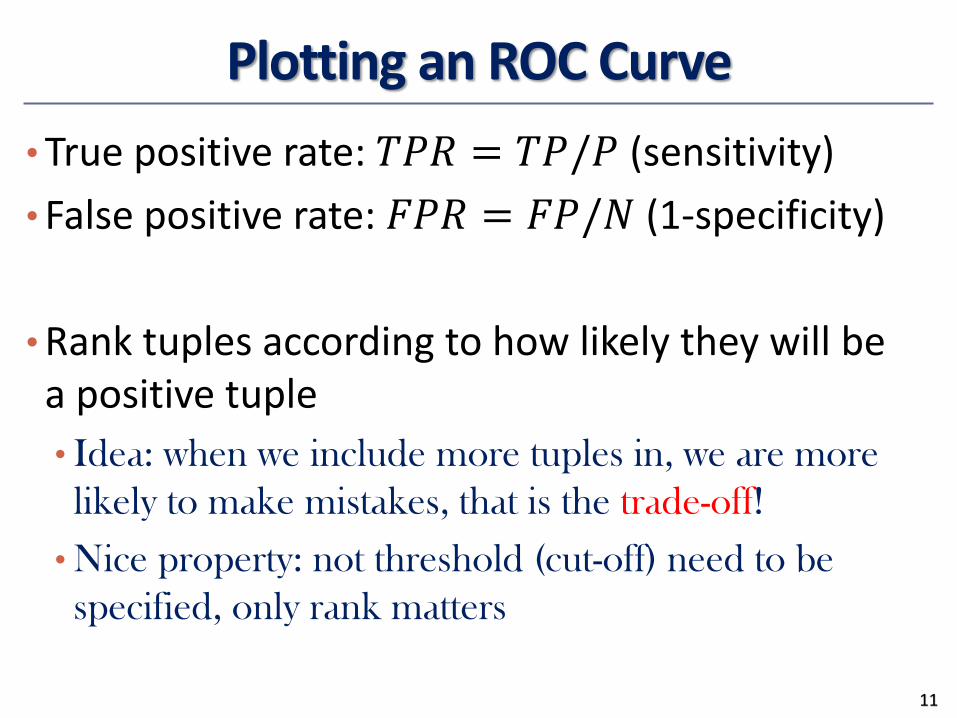
Plotting an ROC Curve

•True positive rate: 𝑇𝑃𝑅 = 𝑇𝑃/𝑃 (sensitivity)

• False positive rate: 𝐹𝑃𝑅 = 𝐹𝑃/𝑁 (1-specificity)

•Rank tuples according to how likely they will be a positive tuple

• Idea: when we include more tuples in, we are more

likely to make mistakes, that is the trade-off!

• Nice property: not threshold (cut-off) need to be

specified, only rank matters

11

12

Example

Evaluation and Other Practical Issues

•Model Evaluation and Selection

•Other issues

•Summary

13

Multiclass Classification

• Multiclass classification

• Classification involving more than two classes (i.e., > 2

Classes)

• Each data point can only belong to one class

• Multilabel classification

• Classification involving more than two classes (i.e., > 2

Classes)

• Each data point can belong to multiple classes

• Can be considered as a set of binary classification

problem

14

Solutions• Method 1. One-vs.-all (OVA): Learn a classifier one at a time

• Given m classes, train m classifiers: one for each class

• Classifier j: treat tuples in class j as positive & all others as negative

• To classify a tuple X, choose the classifier with maximum value

• Method 2. All-vs.-all (AVA): Learn a classifier for each pair of classes

• Given m classes, construct m(m-1)/2 binary classifiers

• A classifier is trained using tuples of the two classes

• To classify a tuple X, each classifier votes. X is assigned to the class with

maximal vote

• Comparison

• All-vs.-all tends to be superior to one-vs.-all

• Problem: Binary classifier is sensitive to errors, and errors affect vote count

15

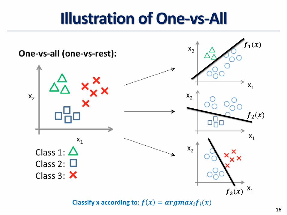
Illustration of One-vs-All

16

𝒇𝟐(𝒙)

𝒇𝟑(𝒙)

𝒇𝟏(𝒙)

Classify x according to: 𝒇 𝒙 = 𝒂𝒓𝒈𝒎𝒂𝒙𝒊𝒇𝒊(𝒙)

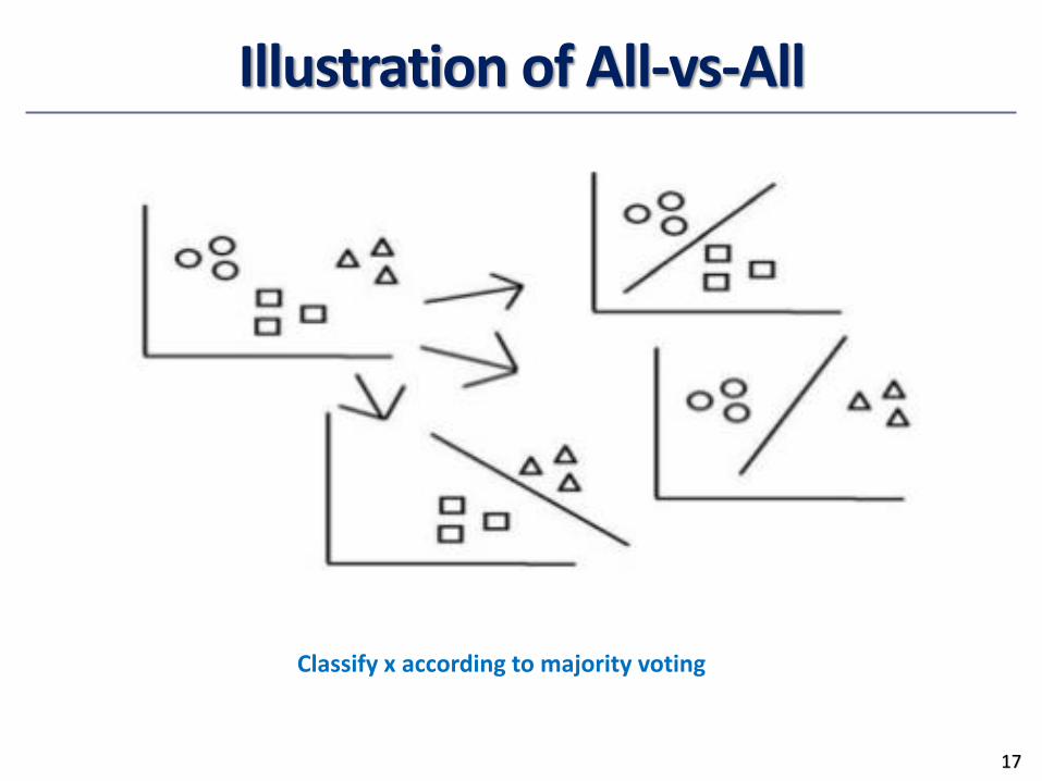
Illustration of All-vs-All

17

Classify x according to majority voting

Extending to Multiclass Classification Directly

•Very straightforward for

•Logistic Regression

•Decision Tree

•Neural Network

•KNN

18

Classification of Class-Imbalanced Data Sets

•Class-imbalance problem• Rare positive example but numerous negative ones,

e.g., medical diagnosis, fraud, oil-spill, fault, etc.

• Traditional methods• Assume a balanced distribution of classes and equal

error costs: not suitable for class-imbalanced data

19

Balanced dataset Imbalanced dataset

How about predicting every data point as blue class?

Solutions

•Pick the right evaluation metric• E.g., ROC is better than accuracy

• Typical methods for imbalance data in 2-class classification (training data): •Oversampling: re-sampling of data from positive class

•Under-sampling: randomly eliminate tuples from negative class

•Synthesizing new data points for minority class

• Still difficult for class imbalance problem on multiclass tasks

20

https://svds.com/learning-imbalanced-classes/

Illustration of Oversampling and Undersampling

21

Illustration of Synthesizing New Data Points

• SMOTE: Synthetic Minority Oversampling Technique (Chawla et. al)

22

Evaluation and Other Practical Issues

•Model Evaluation and Selection

•Other issues

•Summary

23

Summary

•Model evaluation and selection

•Evaluation metric and cross-validation

•Other issues

•Multi-class classification

• Imbalanced classes

24