CS1112 Fall 2010 Project 1 due Thursday 9/9 at 11pm

You must work either on your own or with one partner. You may discuss background issues and general solution

strategies with others, but the project you submit must be the work of just you (and your partner). If you work with

a partner, you and your partner must first register as a group in CMS and then submit your work as a group.

Objectives

Completing this project will help you learn about Matlab scripts, assignment statements, if-else statements,and some Matlab built-in functions. You will also start to explore Matlab graphics.

1 Kepler’s Model of Planetary Orbits

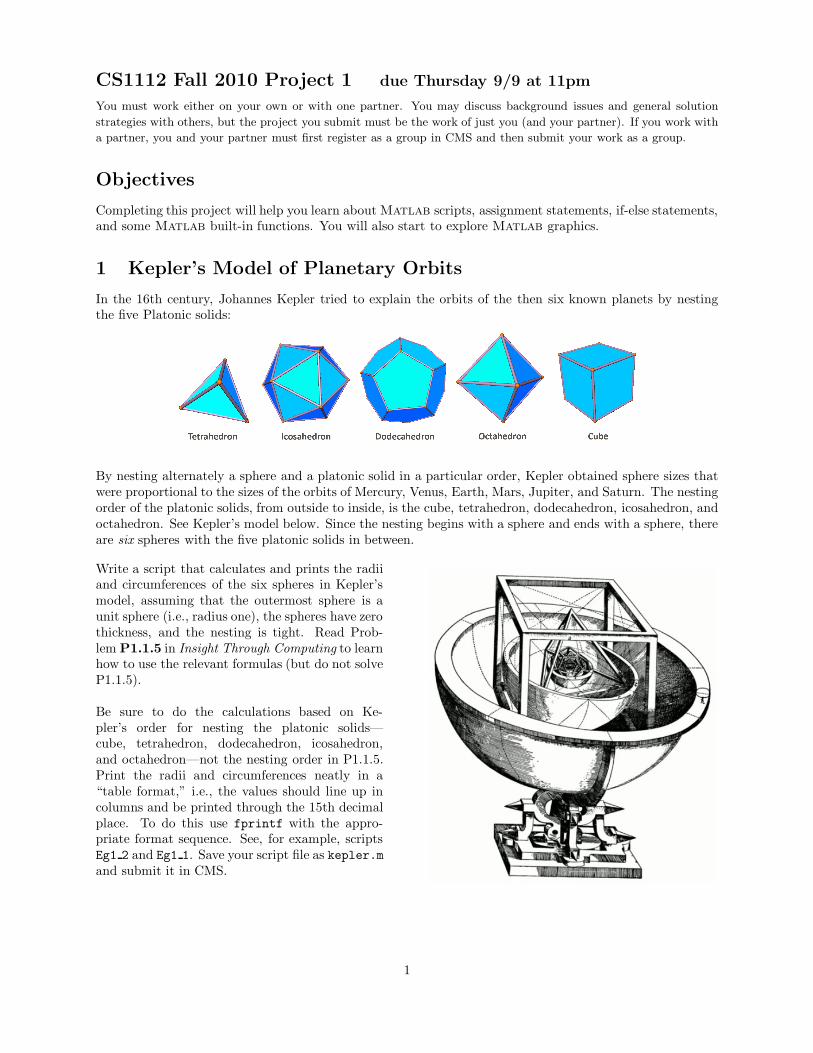
In the 16th century, Johannes Kepler tried to explain the orbits of the then six known planets by nestingthe five Platonic solids:

By nesting alternately a sphere and a platonic solid in a particular order, Kepler obtained sphere sizes thatwere proportional to the sizes of the orbits of Mercury, Venus, Earth, Mars, Jupiter, and Saturn. The nestingorder of the platonic solids, from outside to inside, is the cube, tetrahedron, dodecahedron, icosahedron, andoctahedron. See Kepler’s model below. Since the nesting begins with a sphere and ends with a sphere, thereare six spheres with the five platonic solids in between.

Write a script that calculates and prints the radiiand circumferences of the six spheres in Kepler’smodel, assuming that the outermost sphere is aunit sphere (i.e., radius one), the spheres have zerothickness, and the nesting is tight. Read Prob-lem P1.1.5 in Insight Through Computing to learnhow to use the relevant formulas (but do not solveP1.1.5).

Be sure to do the calculations based on Ke-pler’s order for nesting the platonic solids—cube, tetrahedron, dodecahedron, icosahedron,and octahedron—not the nesting order in P1.1.5.Print the radii and circumferences neatly in a“table format,” i.e., the values should line up incolumns and be printed through the 15th decimalplace. To do this use fprintf with the appro-priate format sequence. See, for example, scriptsEg1 2 and Eg1 1. Save your script file as kepler.mand submit it in CMS.

1

2 Squarish Rectangle

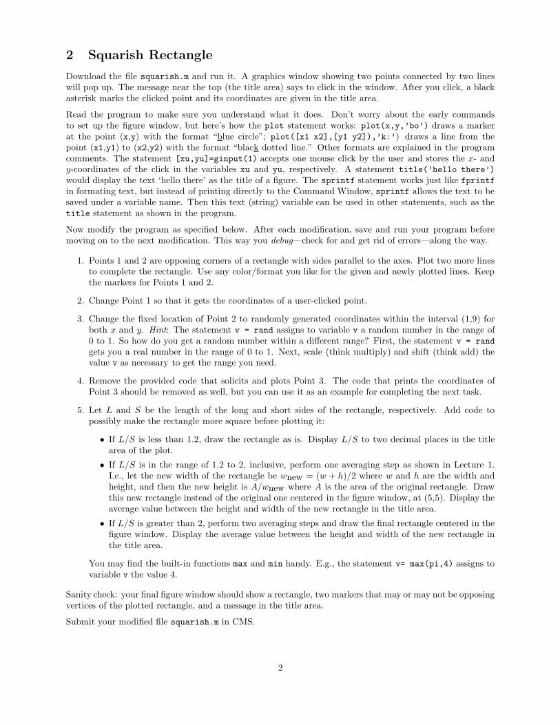
Download the file squarish.m and run it. A graphics window showing two points connected by two lineswill pop up. The message near the top (the title area) says to click in the window. After you click, a blackasterisk marks the clicked point and its coordinates are given in the title area.

Read the program to make sure you understand what it does. Don’t worry about the early commandsto set up the figure window, but here’s how the plot statement works: plot(x,y,’bo’) draws a markerat the point (x,y) with the format “blue circle”; plot([x1 x2],[y1 y2]),’k:’) draws a line from thepoint (x1,y1) to (x2,y2) with the format “black dotted line.” Other formats are explained in the programcomments. The statement [xu,yu]=ginput(1) accepts one mouse click by the user and stores the x- andy-coordinates of the click in the variables xu and yu, respectively. A statement title(’hello there’)would display the text ‘hello there’ as the title of a figure. The sprintf statement works just like fprintfin formating text, but instead of printing directly to the Command Window, sprintf allows the text to besaved under a variable name. Then this text (string) variable can be used in other statements, such as thetitle statement as shown in the program.

Now modify the program as specified below. After each modification, save and run your program beforemoving on to the next modification. This way you debug—check for and get rid of errors—along the way.

1. Points 1 and 2 are opposing corners of a rectangle with sides parallel to the axes. Plot two more linesto complete the rectangle. Use any color/format you like for the given and newly plotted lines. Keepthe markers for Points 1 and 2.

2. Change Point 1 so that it gets the coordinates of a user-clicked point.

3. Change the fixed location of Point 2 to randomly generated coordinates within the interval (1,9) forboth x and y. Hint: The statement v = rand assigns to variable v a random number in the range of0 to 1. So how do you get a random number within a different range? First, the statement v = randgets you a real number in the range of 0 to 1. Next, scale (think multiply) and shift (think add) thevalue v as necessary to get the range you need.

4. Remove the provided code that solicits and plots Point 3. The code that prints the coordinates ofPoint 3 should be removed as well, but you can use it as an example for completing the next task.

5. Let L and S be the length of the long and short sides of the rectangle, respectively. Add code topossibly make the rectangle more square before plotting it:

• If L/S is less than 1.2, draw the rectangle as is. Display L/S to two decimal places in the titlearea of the plot.

• If L/S is in the range of 1.2 to 2, inclusive, perform one averaging step as shown in Lecture 1.I.e., let the new width of the rectangle be wnew = (w + h)/2 where w and h are the width andheight, and then the new height is A/wnew where A is the area of the original rectangle. Drawthis new rectangle instead of the original one centered in the figure window, at (5,5). Display theaverage value between the height and width of the new rectangle in the title area.

• If L/S is greater than 2, perform two averaging steps and draw the final rectangle centered in thefigure window. Display the average value between the height and width of the new rectangle inthe title area.

You may find the built-in functions max and min handy. E.g., the statement v= max(pi,4) assigns tovariable v the value 4.

Sanity check: your final figure window should show a rectangle, two markers that may or may not be opposingvertices of the plotted rectangle, and a message in the title area.

Submit your modified file squarish.m in CMS.

2