CS E6998-1: Advanced Topics inProgramming Languages and Compilers

Alfred V. Ahoaho@cs.columbia.edu

Lecture 1 – Introduction to CourseSeptember 8, 2014

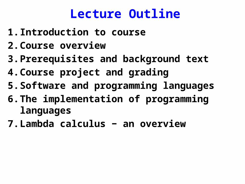
Lecture Outline1. Introduction to course2. Course overview3. Prerequisites and background text4. Course project and grading5. Software and programming languages6. The implementation of programming languages7. Lambda calculus − an overview

1. Introduction to CourseProfessor Al Ahohttp://www.cs.columbia.edu/~aho aho@cs.columbia.eduLectures: Mondays, 4:10-6:00pm, 253 ENGOffice hours: Mondays 3:00-4:00pm, 513 Computer Science BuildingCourse webpage:

http://www.cs.columbia.edu/~aho/cs6998

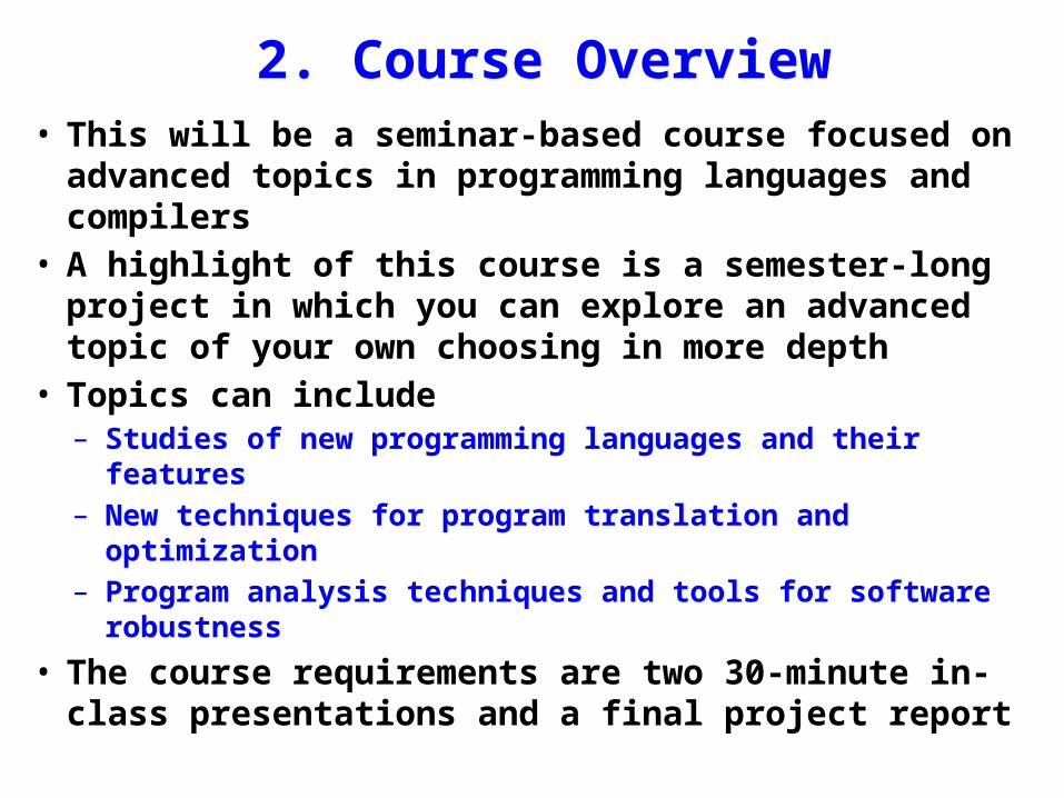
2. Course Overview• This will be a seminar-based course focused on advanced

topics in programming languages and compilers• A highlight of this course is a semester-long project in

which you can explore an advanced topic of your own choosing in more depth

• Topics can include– Studies of new programming languages and their features– New techniques for program translation and optimization – Program analysis techniques and tools for software robustness

• The course requirements are two 30-minute in-class presentations and a final project report

Course Objectives• Understanding how language and compiler technology

can be used to make safer software more reliably and quickly

• Learning the advanced concepts and design principles underlying modern programming languages

• Understanding program analysis techniques and tools• Harnessing language and compiler technology in dealing

with parallelism and concurrency• Experiencing an in-depth project exploring modern

language and compiler techniques

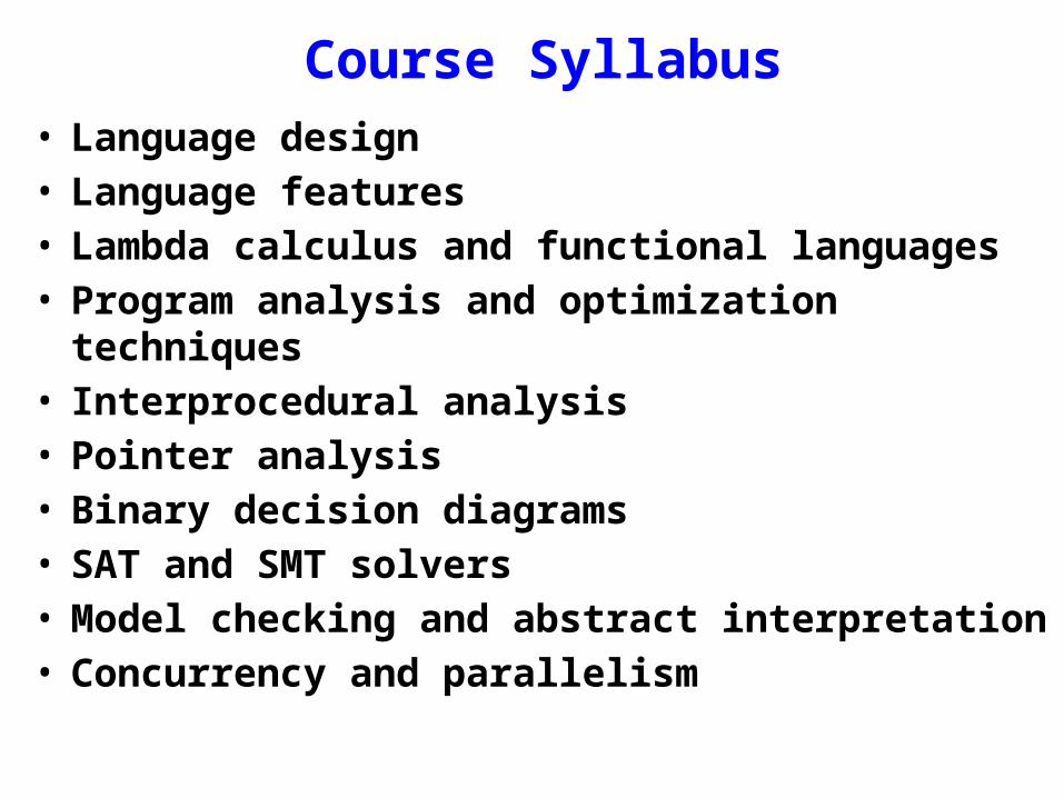
Course Syllabus• Language design• Language features• Lambda calculus and functional languages• Program analysis and optimization techniques• Interprocedural analysis• Pointer analysis• Binary decision diagrams• SAT and SMT solvers• Model checking and abstract interpretation• Concurrency and parallelism

3. Prerequisites and Background Text

• Fluency in at least one major programming language such as C, C++, C#, Java, OCaml, or Python

• COMS W4115: Programming Languages and Translators, or equivalent

• Text: Compilers, Techniques, and Tools(Second Edition), Aho, Lam, Sethi, andUllman, Addison-Wesley, 2007

4. Course Project and Grade

• Each student should select by 9/22/14 a semester-long programming language or compiler project to pursue in more depth. Teams of two are permitted if desired.

• Each student will give two 30-minute presentations to the class

• At the end of the semester, students will submit a final project report summarizing their project.

• The project and classroom discussions will determine the final grade:– 50% for the two presentations– 50% for the final project report

Potential Project Topics• Detailed report on a new PL such as Swift or Java 8• New features being added to legacy PLs• Advanced program analysis and optimization techniques• Solver-aided languages• Verifying compilers• Abstract interpretation and model checking• Regular expression pattern matching in PLs• Applications of category theory to PLs• Insecure constructs in PLs and how to overcome them• Report on a “most influential PLDI paper”– http://www.sigplan.org/Awards/Conferences/PLDI/Main.htm

Recent Most Influential PLDI Papers• Scalable lock-free dynamic memory allocation• The nesC language: a holistic approach to networked embedd

ed systems• Extended static checking for Java• Automatic predicate abstraction of C programs • Dynamo: A transparent dynamic optimization system • A fast Fourier transform compiler • The implementation of the Cilk-5 multithreaded language • Exploiting hardware performance c

ounters with flow and context sensitive profiling• TIL: A type-directed optimizing compiler for ML • Selective specialization for object-oriented languages

[http://www.sigplan.org/Awards/Conferences/PLDI/Main]

5. Software and Programming LanguagesHow much software does the world use today?

Guesstimate: around one trillion lines of source code

What is the sunk cost of the legacy software base?

$100 per line of finished, tested source code

How many bugs are there in the legacy base?

10 to 10,000 defects per million lines of source code

Issues in Programming Language Design• Domain of application– exploit domain restrictions for expressiveness, performance

• Computational model– simplicity, ease of expression

• Abstraction mechanisms– reuse, suggestivity

• Type system– reliability, security

• Usability– readability, writability, efficiency, learnability, scalability, portability

Kinds of Languages - I• Declarative– Program specifies what computation is to be done– Examples: Haskell, ML, Prolog

• Domain specific– Many areas have special-purpose languages for

creating applications– Examples: Lex for scanners, Yacc for parsers

• Functional– One whose computational model is based on lambda

calculus– Examples: Haskell, ML

Kinds of Languages - II• Imperative– Program specifies how a computation is to be done– Examples: C, C++, C#, Fortran, Java

• Markup– One designed for the presentation of text– Usually not Turing complete– Examples: HTML, XHTML, XML

• Object oriented– Program consists of interacting objects– Uses encapsulation, modularity, polymorphism, and

inheritance– Examples: C++, C#, Java, OCaml, Smalltalk

Kinds of Languages - III• Parallel– One that allows a computation to run concurrently on multiple

processors– Examples: CUDA, Cilk, MPI, POSIX threads, X10

• Scripting– An interpreted language with high-level operators for “gluing

together” computations– Examples: Awk, Perl, PHP, Python, Ruby

• von Neumann– One whose computational model is based on the von Neumann

architecture– Computation is done by modifying variables– Examples: C, C++. C#, Fortran, Java

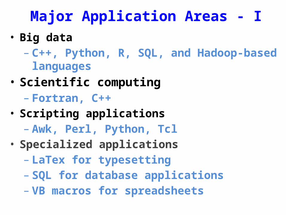
Major Application Areas - I• Big data– C++, Python, R, SQL, and Hadoop-based languages

• Scientific computing– Fortran, C++

• Scripting applications– Awk, Perl, Python, Tcl

• Specialized applications– LaTex for typesetting– SQL for database applications– VB macros for spreadsheets

Major Application Areas - II• Symbolic programming– F#, Haskell, Lisp, ML, Ocaml

• Systems programming– C, C++, C#, Java, Objective-C

• Web programming– CGI– HTML– JavaScript– Ruby on Rails

• Countless other application areas

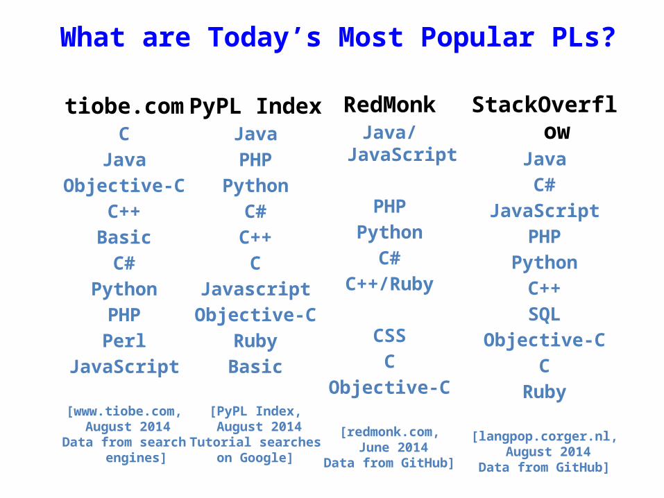
tiobe.comC

JavaObjective-C

C++Basic

C#Python

PHPPerl

JavaScript

[www.tiobe.com, August 2014

Data from search engines]

PyPL IndexJavaPHP

PythonC#

C++C

JavascriptObjective-C

RubyBasic

[PyPL Index, August 2014

Tutorial searcheson Google]

What are Today’s Most Popular PLs?

RedMonkJava/JavaScript

PHPPython

C#C++/Ruby

CSSC

Objective-C

[redmonk.com, June 2014

Data from GitHub]

StackOverflowJavaC#

JavaScriptPHP

PythonC++SQL

Objective-CC

Ruby

[langpop.corger.nl, August 2014

Data from GitHub]

Evolutionary Forces Driving PL Changes

Increasing diversity of applications

Stress on increasing programmer productivity and shortening time to market

Need to improve software security, reliability and maintainability

Emphasis on mobility and distribution

Support for parallelism and concurrency

New mechanisms for modularity and scalability

Trend toward multi-paradigm programming

Target Languages and Machines

Another programming language

CISCs

RISCs

Parallel machines

Multicores

GPUs

Quantum computers

• Ruby is a dynamic, OO scripting language designed by Yukihiro Matsumoto in Japan in the mid 1990s

• Characteristics: object oriented, dynamic, designed for the web, scripting, reflective

• Supports multiple programming paradigms including functional, object oriented, and imperative

• The three pillars of Ruby– everything is an object– every operation is a method call– all programming is metaprogramming

• Made popular by the web application framework Rails

http://www.ruby-lang.org/en/about/

Case Study 1: Ruby

• Scala is a multi-paradigm programming language designed by Martin Odersky at EPFL starting in 2001

• Characteristics: scalable, object oriented, functional, seamless Java interoperability, functions are objects, future-proof, fun

• Integrates functional, imperative and object-oriented programming in a statically typed language

• Functional constructs used for parallelism and distributed computing

• Generates Java byte code• Used to implement Twitter

– Katy Perry has 54 million followers– Barack Obama has 44 million followers

[http://twitaholic.com/]

http://www.scala-lang.org/what-is-scala.html

Case Study 2: Scala

How Many PLs are There?

Guesstimate: thousands

The website http://www.99-bottles-of-beer.net has programs in over 1,500 different programming languages and variations to print the lyrics to the song “99 Bottles of Beer.”

“99 Bottles of Beer”99 bottles of beer on the wall, 99 bottles of beer.Take one down and pass it around, 98 bottles of beer on the wall.

98 bottles of beer on the wall, 98 bottles of beer.Take one down and pass it around, 97 bottles of beer on the wall.

.

.

.2 bottles of beer on the wall, 2 bottles of beer.Take one down and pass it around, 1 bottle of beer on the wall.

1 bottle of beer on the wall, 1 bottle of beer.Take one down and pass it around, no more bottles of beer on

the wall.

No more bottles of beer on the wall, no more bottles of beer.Go to the store and buy some more, 99 bottles of beer on the

wall.[Traditional]

“99 Bottles of Beer” in AWK

BEGIN { for(i = 99; i >= 0; i--) { print ubottle(i), "on the wall,", lbottle(i) "." print action(i), lbottle(inext(i)), "on the wall." print }}function ubottle(n) { return sprintf("%s bottle%s of beer", n ? n : "No more", n - 1 ? "s" : "")}function lbottle(n) { return sprintf("%s bottle%s of beer", n ? n : "no more", n - 1 ? "s" : "")}function action(n) { return sprintf("%s", n ? "Take one down and pass it around," : \ "Go to the store and buy some more,")}function inext(n) { return n ? n - 1 : 99}

[Osamu Aoki, http://people.debian.org/~osamu]

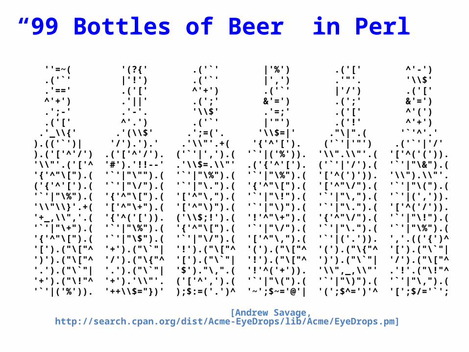
“99 Bottles of Beer” in Perl

''=~( '(?{' .('`' |'%') .('[' ^'-') .('`' |'!') .('`' |',') .'"'. '\\$' .'==' .('[' ^'+') .('`' |'/') .('[' ^'+') .'||' .(';' &'=') .(';' &'=') .';-' .'-'. '\\$' .'=;' .('[' ^'(') .('[' ^'.') .('`' |'"') .('!' ^'+') .'_\\{' .'(\\$' .';=('. '\\$=|' ."\|".( '`'^'.' ).(('`')| '/').').' .'\\"'.+( '{'^'['). ('`'|'"') .('`'|'/' ).('['^'/') .('['^'/'). ('`'|',').( '`'|('%')). '\\".\\"'.( '['^('(')). '\\"'.('['^ '#').'!!--' .'\\$=.\\"' .('{'^'['). ('`'|'/').( '`'|"\&").( '{'^"\[").( '`'|"\"").( '`'|"\%").( '`'|"\%").( '['^(')')). '\\").\\"'. ('{'^'[').( '`'|"\/").( '`'|"\.").( '{'^"\[").( '['^"\/").( '`'|"\(").( '`'|"\%").( '{'^"\[").( '['^"\,").( '`'|"\!").( '`'|"\,").( '`'|(',')). '\\"\\}'.+( '['^"\+").( '['^"\)").( '`'|"\)").( '`'|"\.").( '['^('/')). '+_,\\",'.( '{'^('[')). ('\\$;!').( '!'^"\+").( '{'^"\/").( '`'|"\!").( '`'|"\+").( '`'|"\%").( '{'^"\[").( '`'|"\/").( '`'|"\.").( '`'|"\%").( '{'^"\[").( '`'|"\$").( '`'|"\/").( '['^"\,").( '`'|('.')). ','.(('{')^ '[').("\["^ '+').("\`"| '!').("\["^ '(').("\["^ '(').("\{"^ '[').("\`"| ')').("\["^ '/').("\{"^ '[').("\`"| '!').("\["^ ')').("\`"| '/').("\["^ '.').("\`"| '.').("\`"| '$')."\,".( '!'^('+')). '\\",_,\\"' .'!'.("\!"^ '+').("\!"^ '+').'\\"'. ('['^',').( '`'|"\(").( '`'|"\)").( '`'|"\,").( '`'|('%')). '++\\$="})' );$:=('.')^ '~';$~='@'| '(';$^=')'^ '[';$/='`';

[Andrew Savage, http://search.cpan.org/dist/Acme-EyeDrops/lib/Acme/EyeDrops.pm]

“99 Bottles of Beer” in the Whitespace Language

[Andrew Kemp, http://compsoc.dur.ac.uk/whitespace]

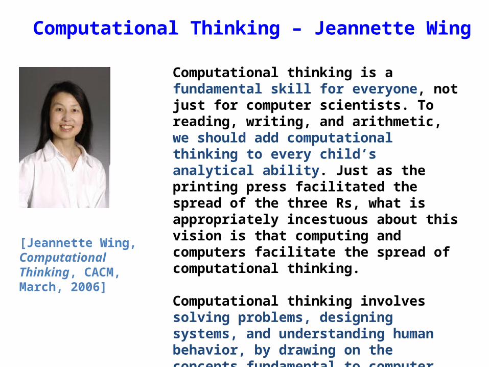
Computational Thinking – Jeannette Wing

Computational thinking is a fundamental skill for everyone, not just for computer scientists. To reading, writing, and arithmetic, we should add computational thinking to every child’s analytical ability. Just as the printing press facilitated the spread of the three Rs, what is appropriately incestuous about this vision is that computing and computers facilitate the spread of computational thinking.

Computational thinking involves solving problems, designing systems, and understanding human behavior, by drawing on the concepts fundamental to computer science. Computational thinking includes a range of mental tools that reflect the breadth of the field of computer science.

[Jeannette Wing, Computational Thinking, CACM, March, 2006]

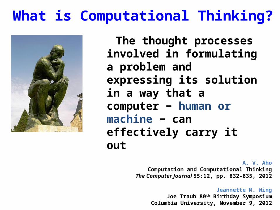
What is Computational Thinking?

The thought processes involved in formulating a problem and expressing its solution in a way that a computer − human or machine − can effectively carry it out

A. V. AhoComputation and Computational Thinking

The Computer Journal 55:12, pp. 832-835, 2012

Jeannette M. WingJoe Traub 80th Birthday Symposium

Columbia University, November 9, 2012

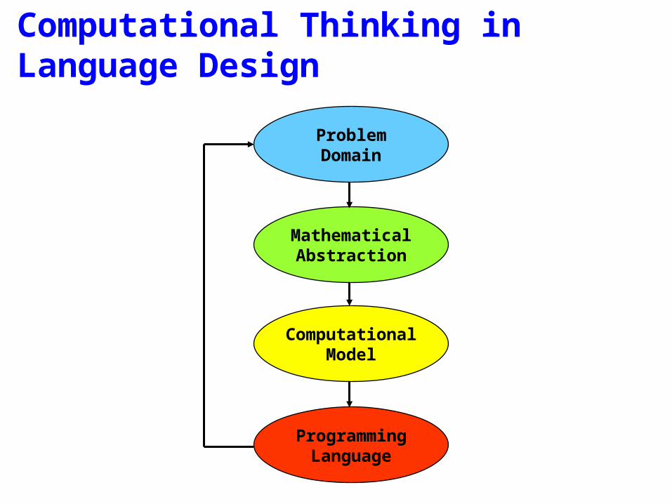
Computational Thinking in Language Design

ProblemDomain

MathematicalAbstraction

ComputationalModel

ProgrammingLanguage

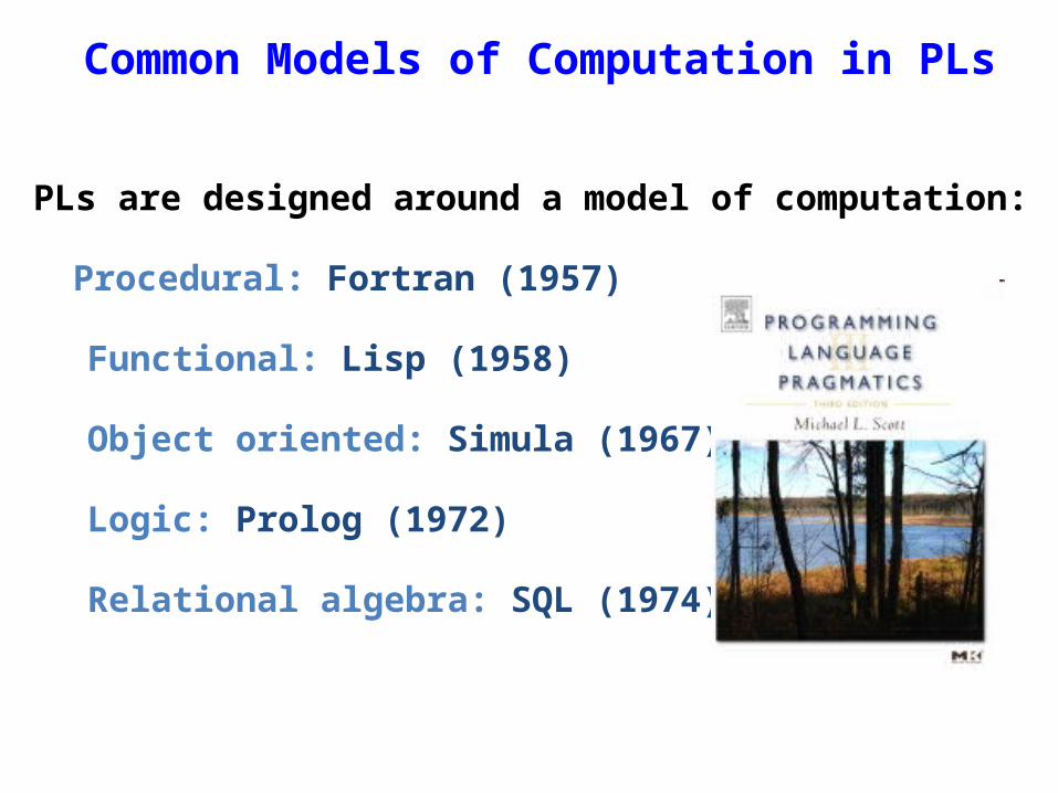
Common Models of Computation in PLs

PLs are designed around a model of computation:

Procedural: Fortran (1957)

Functional: Lisp (1958)

Object oriented: Simula (1967)

Logic: Prolog (1972)

Relational algebra: SQL (1974)

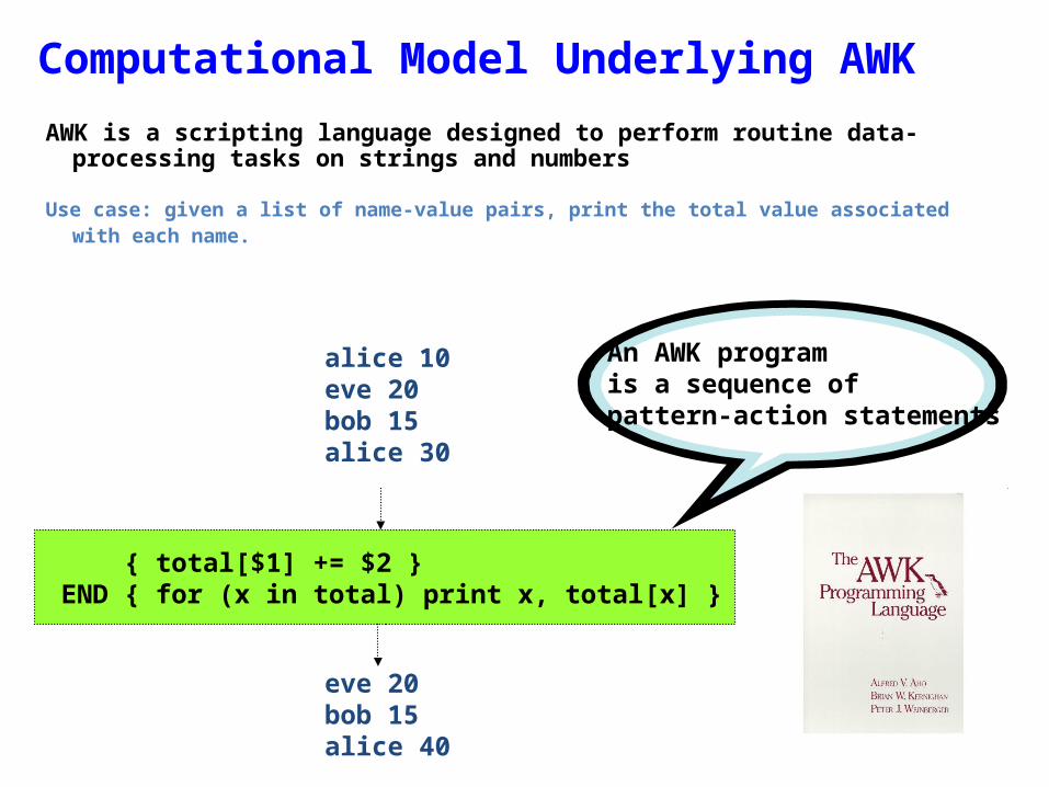
AWK is a scripting language designed to perform routine data-processing tasks on strings and numbers

Use case: given a list of name-value pairs, print the total value associated with each name.

Computational Model Underlying AWK

eve 20 bob 15 alice 40

alice 10 eve 20 bob 15 alice 30

{ total[$1] += $2 } END { for (x in total) print x, total[x] }

An AWK programis a sequence ofpattern-action statements

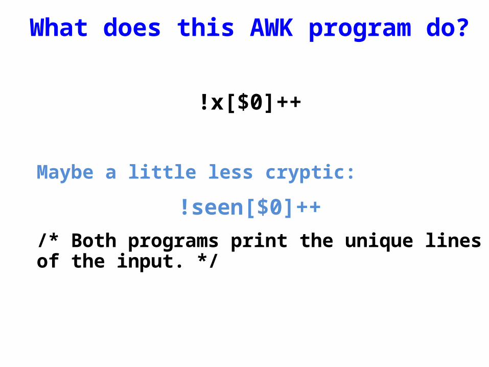
What does this AWK program do?

!x[$0]++

Maybe a little less cryptic:

!seen[$0]++

/* Both programs print the unique lines of the input. */

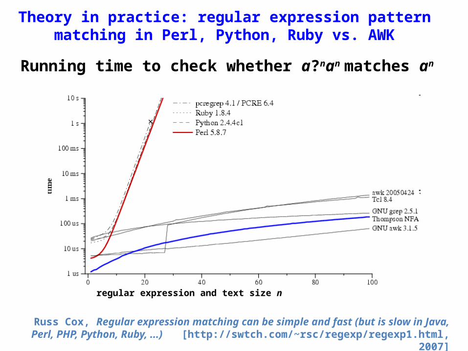
Theory in practice: regular expression pattern matching in Perl, Python, Ruby vs. AWK

Running time to check whether a?nan matches an

regular expression and text size n

Russ Cox, Regular expression matching can be simple and fast (but is slow in Java, Perl, PHP, Python, Ruby, ...) [http://swtch.com/~rsc/regexp/regexp1.html, 2007]

The Specification of PLs

• Syntax

• Semantics

• Pragmatics

• However, a precise, automatable, easy-to-understand, easy-to-implement method for specifying a complete language is still an open research problem

Grammars are Used to Help Specify SyntaxThe grammar S → aSbS | bSaS | ε generates all strings of a’s and b’s

with the same number of a’s as b’s.

This grammar is ambiguous: abab has two parse trees.

S

a

b S a S ε

S b S

ε ε

(ab)n has parse trees

n

n

n

2

1

1

S

SbSaε

a S b S

ε ε

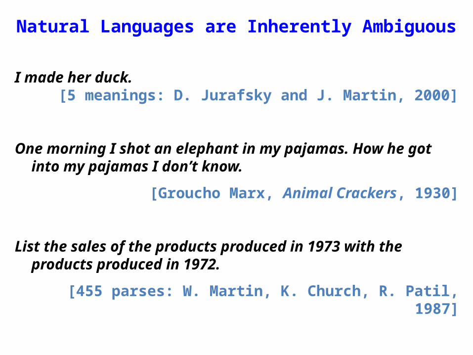
Natural Languages are Inherently Ambiguous

I made her duck.[5 meanings: D. Jurafsky and J. Martin, 2000]

One morning I shot an elephant in my pajamas. How he got into my pajamas I don’t know.

[Groucho Marx, Animal Crackers, 1930]

List the sales of the products produced in 1973 with the products produced in 1972.

[455 parses: W. Martin, K. Church, R. Patil, 1987]

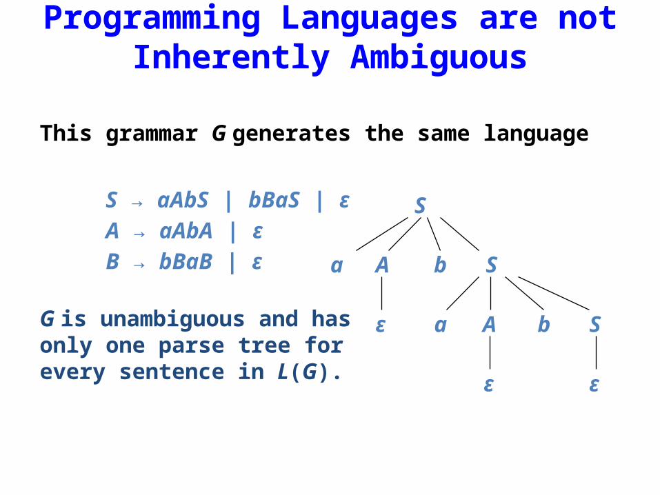
Programming Languages are notInherently Ambiguous

This grammar G generates the same language

S → aAbS | bBaS | εA → aAbA | εB → bBaB | ε

G is unambiguous and hasonly one parse tree forevery sentence in L(G).

S

SbAaε

a A b S

ε ε

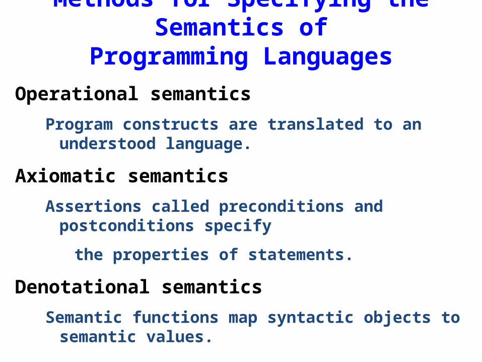
Methods for Specifying the Semantics ofProgramming Languages

Operational semantics

Program constructs are translated to an understood language.

Axiomatic semantics

Assertions called preconditions and postconditions specify

the properties of statements.

Denotational semantics

Semantic functions map syntactic objects to semantic values.

6. The Implementation of PLs

• Compilers

• Interpreters

• Just-in-time compilers

• Compiler collections such as GCC and LLVM

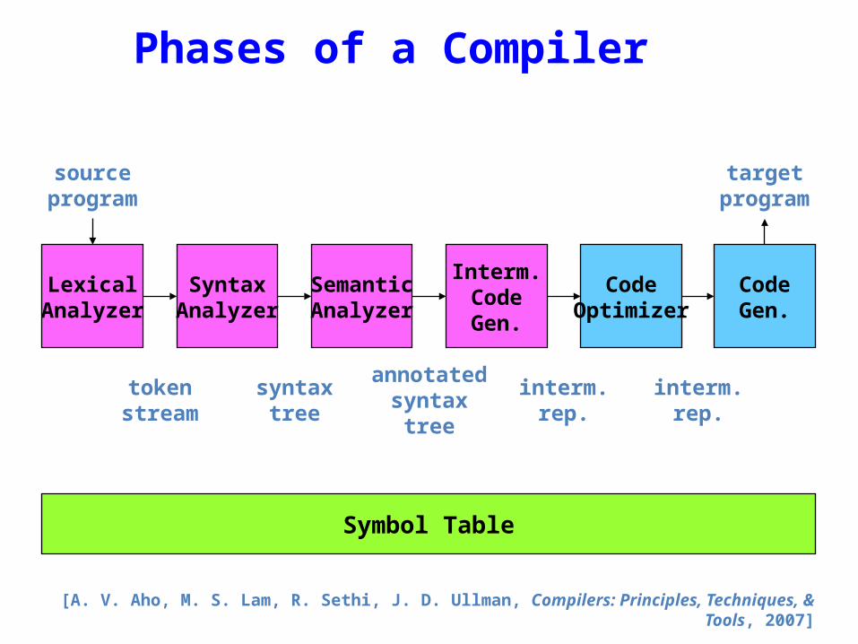
Phases of a Compiler

SemanticAnalyzer

Interm.CodeGen.

SyntaxAnalyzer

LexicalAnalyzer

CodeOptimizer

CodeGen.

sourceprogram

tokenstream

syntaxtree

annotatedsyntax

tree

interm.rep.

interm.rep.

targetprogram

Symbol Table

[A. V. Aho, M. S. Lam, R. Sethi, J. D. Ullman, Compilers: Principles, Techniques, & Tools, 2007]

Compiler Component Generators

SyntaxAnalyzer

LexicalAnalyzer

sourceprogram

tokenstream

syntaxtree

LexicalAnalyzer

Generator(lex)

SyntaxAnalyzer

Generator(yacc)

lexspecification

yaccspecification

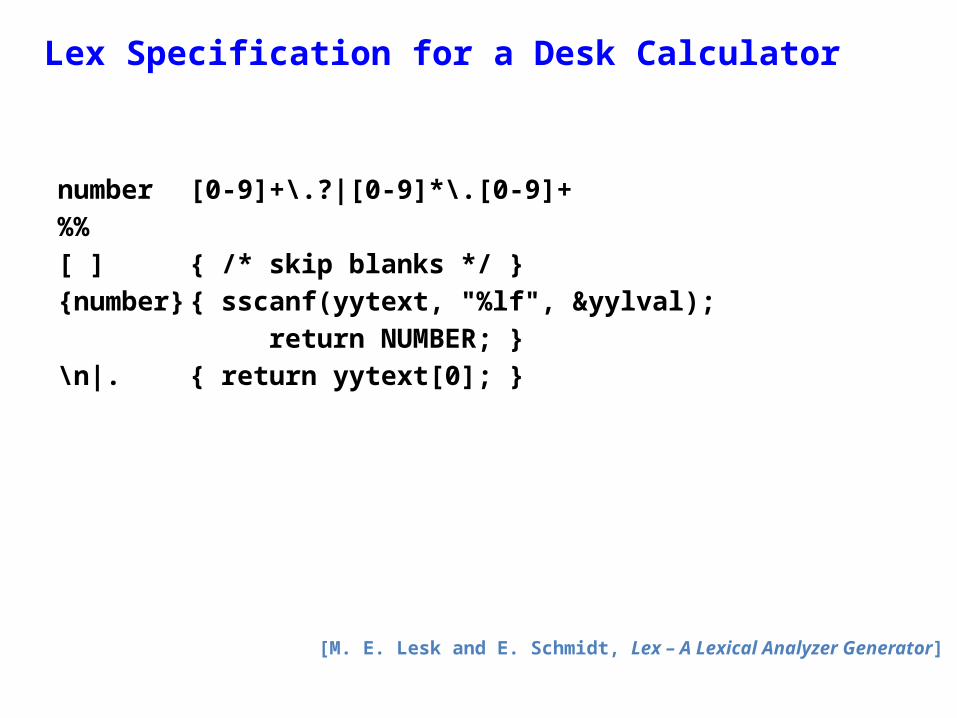
Lex Specification for a Desk Calculator

number [0-9]+\.?|[0-9]*\.[0-9]+%%[ ] { /* skip blanks */ }{number}{ sscanf(yytext, "%lf", &yylval);

return NUMBER; }\n|. { return yytext[0]; }

[M. E. Lesk and E. Schmidt, Lex – A Lexical Analyzer Generator]

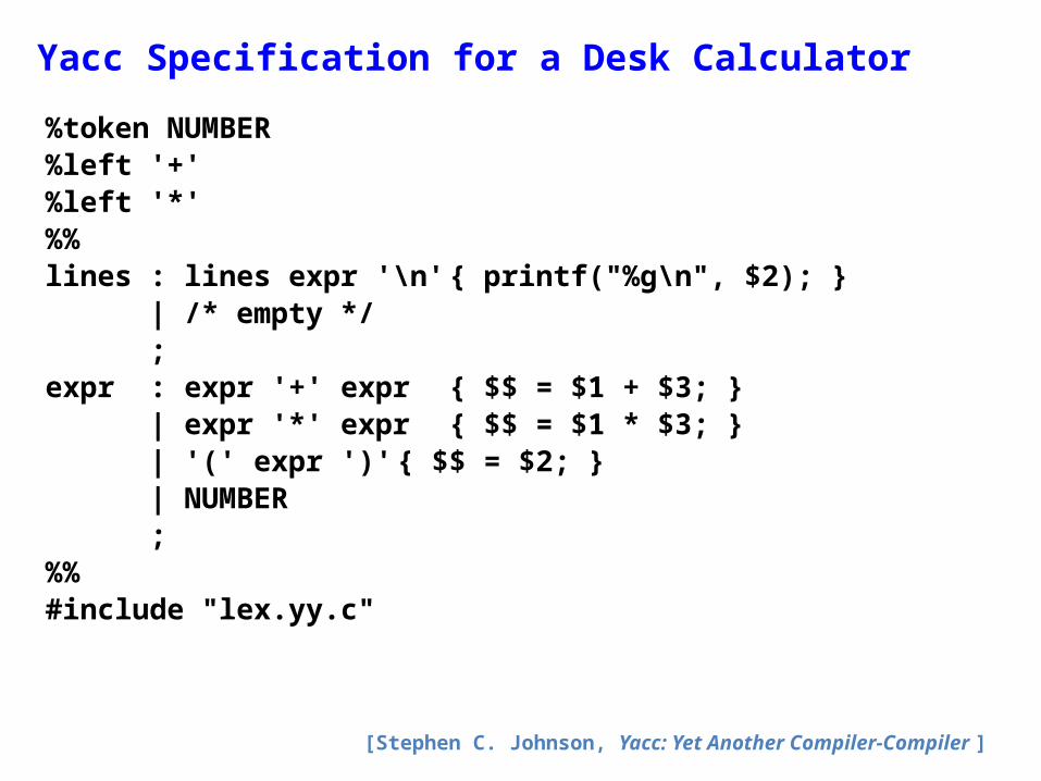
Yacc Specification for a Desk Calculator%token NUMBER%left '+'%left '*'%%lines : lines expr '\n' { printf("%g\n", $2); } | /* empty */ ;expr : expr '+' expr { $$ = $1 + $3; } | expr '*' expr { $$ = $1 * $3; } | '(' expr ')'{ $$ = $2; } | NUMBER ;%%#include "lex.yy.c"

[Stephen C. Johnson, Yacc: Yet Another Compiler-Compiler ]

Creating the Desk Calculator

Invoke the commandslex desk.lyacc desk.ycc y.tab.c –ly –ll

Result

DeskCalculator1.2 * (3.4 + 5.6) 10.8

Some Computational Thinking Lessons Learned in COMS W4115

• “Designing a language is hard and designing a simple language is extremely hard!”

• “During this course we realized how naïve and overambitious we were, and we all gained a newfound respect for the work and good decisions that went into languages like C and Java which we’ve taken for granted for years.”

7. Lambda Calculus − An Overview

• Lambda calculus was introduced in the 1930s by Alonzo Church as a mathematical system for defining computable functions.

• Lambda calculus is equivalent in definitional power to that of Turing machines.

• Lambda calculus serves as the computational model underlying functional programming languages.

• Lisp was developed by John McCarthy in 1956 around lambda calculus. • ML, a general purpose functional programming language, was developed

by Robin Milner in the late 1970s. • Haskell, considered by many as one of the purest functional

programming languages, was developed by Simon Peyton Jones, Paul Houdak, Phil Wadler and others in the late 1980s and early 90s.

• Features from lambda calculus such as lambda expressions have been incorporated into many widely used programming languages like C++ and Java 8.

Grammar for Lambda Calculus

• The central concept in lambda calculus is an expression which can denote a function definition (called a function abstraction) or a function application.

expr → abstraction | application | (expr) | var | constant

abstraction → λ var . exprapplication → expr expr

• We can think of a lambda-calculus expression as a program which when evaluated returns a result consisting of another lambda-calculus expression.

• For notational convenience, we have included constants that can be numbers and built-in functions. These are unnecessary – they can be simulated in pure lambda calculus.

Function Abstraction

• A function abstraction, often called a lambda abstraction, is an expression defining a function.

• It consists of a lambda followed by a variable, a period, and then an expression: λ var . expr

• In the function λ var . expr, var is the formal parameter and expr the body.

• We say λ var . expr binds var in expr. • Example

– λx.y is a function abstraction. – The variable x after the λ is the formal parameter of the function. – The expression y after the period is the body of the function.

Function Application and Currying

• A function application, often called a lambda application, consists of an expression followed by an expression: expr expr.

• If f is a function and x an expression, then fx is a function application denoting the application of the function f to the argument x. All functions in lambda calculus are prefix.

• If we want to apply a function to more than one argument, we can use a technique called currying. We can express the sum of 1 and 2 by writing ((+ 1) 2). The expression (+ 1) denotes the function that adds 1 to its argument. Thus ((+ 1) 2) means the function + is applied to the argument 1 and the result is a function that is applied to 2.

Lambda Calculus Conventions

• As in ordinary mathematics, we can omit redundant parentheses to avoid cluttering up expressions so we often write ((+ 1) 2) as (+ 1 2) or even + 1 2.

• Function application is left associative and application binds tighter than period. – Example: λx.fgx = (λx.(fg)x)– Example: (λx.λy.xy)λz.z = (λx.(λy.(xy)))λz.z

• The body in a function abstraction extends as far to the right as possible.– Example: λx.+ x 1 = λx.(+ x 1)

Evaluating an Expression

• A lambda calculus expression can be thought of as a program which can be executed by evaluating it. Evaluation is done by repeatedly finding a reducible expression (called a redex) and reducing it using a technique called beta reduction.

• For example the lambda calculus expression (+ (* 1 2) (* 3 4))

has two redexes: (* 1 2) and (* 3 4)

• If we choose to reduce the first redex and then the second and then the result, we get the following sequence of reductions:

(+ (* 1 2) (* 3 4)) → (+ 2 (* 3 4)) → (+ 2 12) → 14

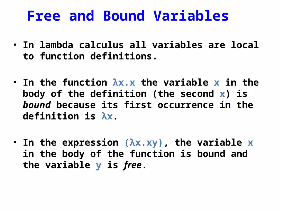
Free and Bound Variables

• In lambda calculus all variables are local to function definitions.

• In the function λx.x the variable x in the body of the definition (the second x) is bound because its first occurrence in the definition is λx.

• In the expression (λx.xy), the variable x in the body of the function is bound and the variable y is free.

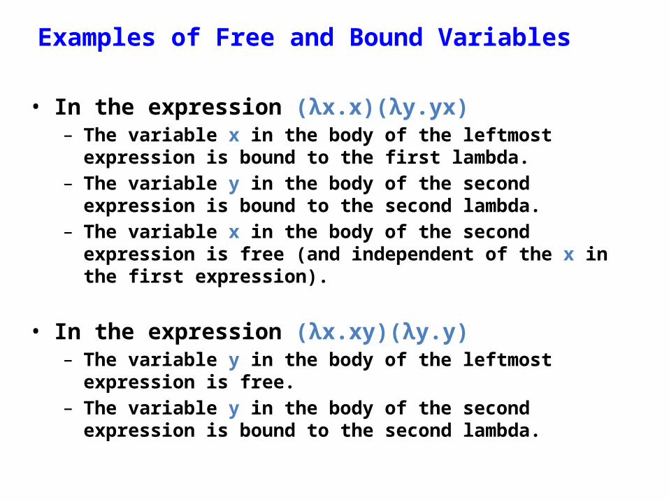
Examples of Free and Bound Variables

• In the expression (λx.x)(λy.yx)– The variable x in the body of the leftmost expression is bound to the

first lambda. – The variable y in the body of the second expression is bound to the

second lambda. – The variable x in the body of the second expression is free (and

independent of the x in the first expression).

• In the expression (λx.xy)(λy.y)– The variable y in the body of the leftmost expression is free. – The variable y in the body of the second expression is bound to the

second lambda.

The Set of Free Variables

• Given an expression e, the following rules define FV(e), the set of free variables in e: – If e is a variable x, then FV(e) = {x}.– If e is of the form λx.y, then FV(e) = FV(y) − {x}.– If e is of the form xy, then FV(e) = FV(x) FV(∪ y).

• An expression with no free variables is said to be closed.

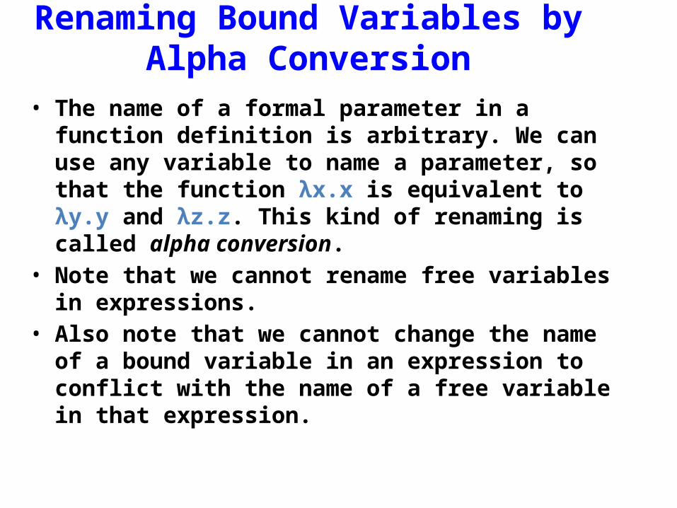
Renaming Bound Variables byAlpha Conversion

• The name of a formal parameter in a function definition is arbitrary. We can use any variable to name a parameter, so that the function λx.x is equivalent to λy.y and λz.z. This kind of renaming is called alpha conversion.

• Note that we cannot rename free variables in expressions. • Also note that we cannot change the name of a bound

variable in an expression to conflict with the name of a free variable in that expression.

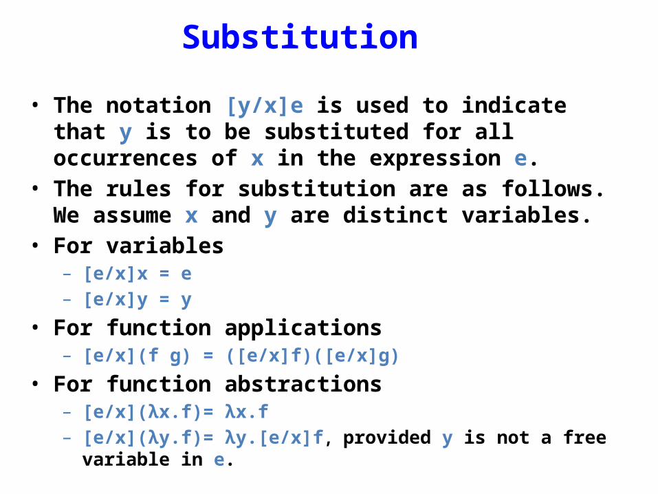
Substitution

• The notation [y/x]e is used to indicate that y is to be substituted for all occurrences of x in the expression e.

• The rules for substitution are as follows. We assume x and y are distinct variables.

• For variables – [e/x]x = e– [e/x]y = y

• For function applications – [e/x](f g) = ([e/x]f)([e/x]g)

• For function abstractions – [e/x](λx.f)= λx.f– [e/x](λy.f)= λy.[e/x]f, provided y is not a free variable in e.

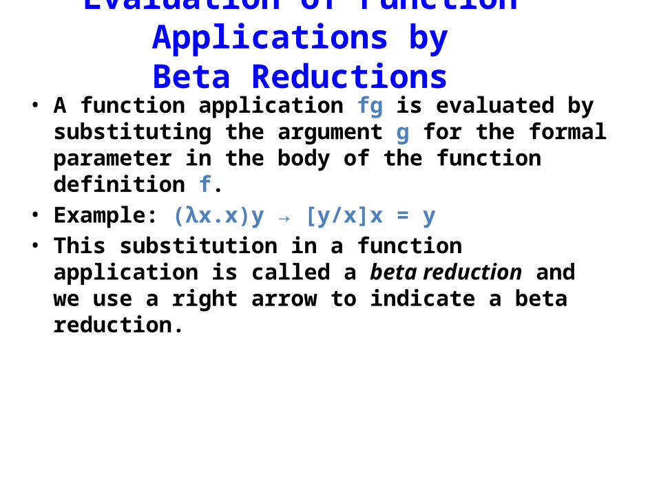
Evaluation of Function Applications byBeta Reductions

• A function application fg is evaluated by substituting the argument g for the formal parameter in the body of the function definition f.

• Example: (λx.x)y → [y/x]x = y • This substitution in a function application is called a beta

reduction and we use a right arrow to indicate a beta reduction.

Function Application by Beta Reductions

• If expr1 → expr2, we say expr1 reduces to expr2 in one step.

• In general, (λx.e)g → [g/x]e means that applying the function (λx.e) to the argument expression g reduces to the function body [g/x]e after substituting the argument expression g for the function's formal parameter x in the function body e.

• We use →* to denote the reflexive and transitive closure of →.

Eta Conversion and Beta Abstraction

• The two lambda expressions (λx.+ 1 x) and (+ 1) are equivalent in the sense that these expressions behave in exactly the same way when they are applied to an argument − they add 1 to it. Eta conversion is a rule that expresses this equivalence.

• In general, if x does not occur free in the function F, then (λx.F x) is eta convertible to F.– Example: (λx.+ 1 x) is eta convertible to (+ 1)

• We will sometimes say + 1 y is a beta abstraction of (λx.+ x y)1. This is analogous to running beta reduction in reverse.

Evaluating Expressions using Renaming

• When performing substitutions, we should be careful to avoid mixing up free occurrences of a variable with bound ones.

• When we apply the function λx.e to an expression g, we

substitute all occurrences of x in e with g. If there is a free variable in g named x, we rename the bound variable x to avoid any conflicts before doing the substitution.

Examples of Evaluating Expressionsusing Renaming

• The expression (λx.(λy.xy))y) contains a bound y in the middle and a free y at the right. We can rename the bound variable y to a new variable, say z, to evaluate the expression with no name conflicts: (λx.(λy.xy))y) =

(λx.(λz.xz))y) → [y/x](λz.xz) = (λz.yz)

• The body of the leftmost expression in (λx.(λy.(x(λx.xy))))y is (λy.(x(λx.xy))). In this body only the first x is free.

Before substituting, we rename the bound variable y to z, say, to avoid confusing it with its free occurrence. Therefore we get the evaluation:

(λx.(λy.(x(λx.xy))))y = (λx.(λz(x(λx.xz))))y → [y/x](λz.(x(λx.xz))) = (λz.(y(λx.xz)))

Normal Forms

• An expression containing no possible beta reductions is called a normal form.

• A normal form expression has no redexes in it. • Examples of normal form expressions: – x where x is a variable – xe where x is a variable and e is a normal form expression – λx.e where x is a variable and e is a normal form

expression

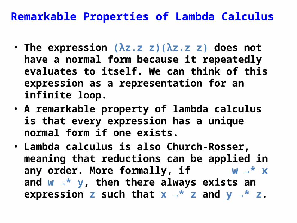
Remarkable Properties of Lambda Calculus

• The expression (λz.z z)(λz.z z) does not have a normal form because it repeatedly evaluates to itself. We can think of this expression as a representation for an infinite loop.

• A remarkable property of lambda calculus is that every expression has a unique normal form if one exists.

• Lambda calculus is also Church-Rosser, meaning that reductions can be applied in any order. More formally, if w →* x and w →* y, then there always exists an expression z such that x →* z and y →* z.

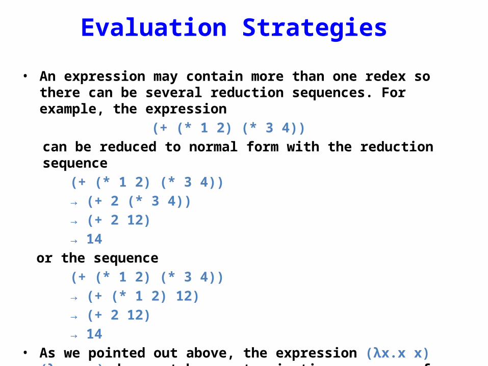
Evaluation Strategies

• An expression may contain more than one redex so there can be several reduction sequences. For example, the expression

(+ (* 1 2) (* 3 4)) can be reduced to normal form with the reduction sequence

(+ (* 1 2) (* 3 4))→ (+ 2 (* 3 4))→ (+ 2 12)→ 14

or the sequence(+ (* 1 2) (* 3 4))→ (+ (* 1 2) 12)→ (+ 2 12)→ 14

• As we pointed out above, the expression (λx.x x)(λx.x x) does not have a terminating sequence of reductions.

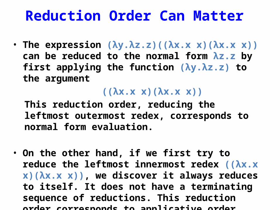
Reduction Order Can Matter

• The expression (λy.λz.z)((λx.x x)(λx.x x)) can be reduced to the normal form λz.z by first applying the function (λy.λz.z) to the argument

((λx.x x)(λx.x x))This reduction order, reducing the leftmost outermost redex, corresponds to normal form evaluation.

• On the other hand, if we first try to reduce the leftmost

innermost redex ((λx.x x)(λx.x x)), we discover it always reduces to itself. It does not have a terminating sequence of reductions. This reduction order corresponds to applicative order evaluation.

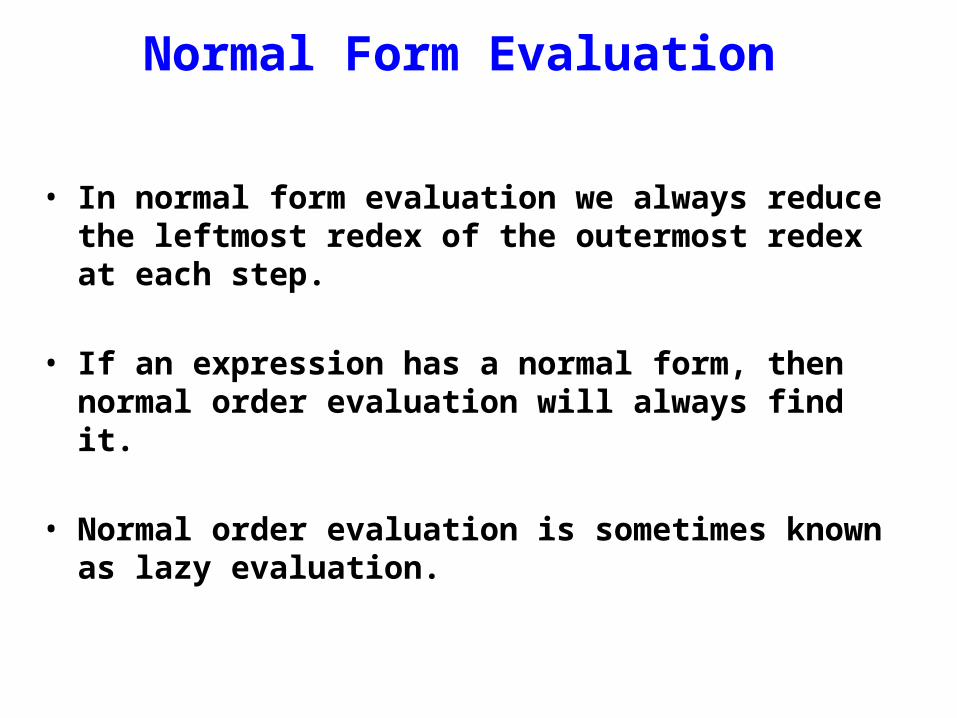
Normal Form Evaluation

• In normal form evaluation we always reduce the leftmost redex of the outermost redex at each step.

• If an expression has a normal form, then normal order

evaluation will always find it.

• Normal order evaluation is sometimes known as lazy evaluation.

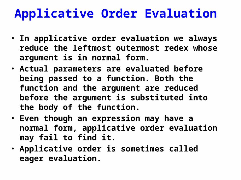
Applicative Order Evaluation

• In applicative order evaluation we always reduce the leftmost outermost redex whose argument is in normal form.

• Actual parameters are evaluated before being passed to a function. Both the function and the argument are reduced before the argument is substituted into the body of the function.

• Even though an expression may have a normal form, applicative order evaluation may fail to find it.

• Applicative order is sometimes called eager evaluation.

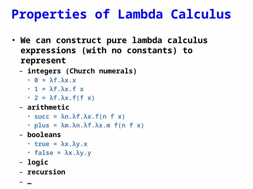
Properties of Lambda Calculus

• We can construct pure lambda calculus expressions (with no constants) to represent– integers (Church numerals)• 0 = λf.λx.x• 1 = λf.λx.f x• 2 = λf.λx.f(f x)

– arithmetic• succ = λn.λf.λx.f(n f x)• plus = λm.λn.λf.λx.m f(n f x)

– booleans• true = λx.λy.x• false = λx.λy.y

– logic– recursion– …

Recursion with the Y Combinator

• The fixed-point Y combinator is a function that takes a function G as an argument and returns G(Y G).

• With repeated applications we can get G(G(Y G)), G(G(G(Y G))), . . .

• We can implement recursive functions by defining the Y combinator: Y = λf.(λx.f(xx))(λx.f(xx))

• Note thatY G = (λf.(λx.f(xx))(λx.f(xx)))G → (λx.G(xx))(λx.G(xx)) → G((λx.G(xx))(λx.G(xx))) = G(Y G)The last line follows from Y G = (λx.G(xx))(λx.G(xx))

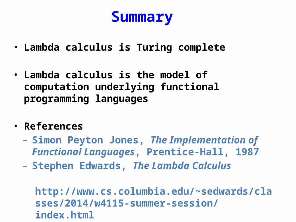
Summary

• Lambda calculus is Turing complete

• Lambda calculus is the model of computation underlying functional programming languages

• References– Simon Peyton Jones, The Implementation of Functional

Languages, Prentice-Hall, 1987– Stephen Edwards, The Lambda Calculus

http://www.cs.columbia.edu/~sedwards/classes/2014/w4115-summer-session/index.html