CS E6204 Lectures 8b and 9a

Knots and Graphs∗

Abstract

Heffter’s invention of rotation systems made it pos-sible to investigate imbeddings of graphs from a pre-dominantly combinatorial perspective. Analogously,the Seifert matrix and the Alexander matrix madeknot theory amenable to algebraic methods. Subse-quently, Conway’s rederivation of the Alexander poly-nomial with skeins and the discovery of the Jones poly-nomial, by Jones, and its subsequent combinatorializa-tion by Kauffman and others has greatly facilitated thecalculation of knot and link invariants.

* Extracted from Chapters 16,17 of Algebraic Graph Theory, byChris Godsil (U of Waterloo) and Gordon Royle (U of WesternAustralia).

1

Knots and Graphs 2

Chapter 16 of Godsil and Royle

1. Knots and their projections

2. Reidemeister moves on knots

3. Signed plane graphs

4. Reidemeister moves on graphs

5. Reidemeister invariants

6. The Kauffman bracket polynomial

7. The Jones polynomial

8. Connectivity

Knots and Graphs 3

1 Knots and Their Projections

A knot is a piecewise-linear (abbr. PL) mapping of the cir-cle S1 into S3. We often refer to the image of a knot as theknot. In dimension 3, the PL category is equivalent to the dif-ferentiable category, so we may think of knots as smoothclosed curves.

A link is a collection of pairwise disjoint knots. For simplicityof exposition, we may sometimes say “knot” when our meaningis either a knot or a link.

A normal projection of a link (aka shadow) is a 4-regulargraph imbedded in the plane.

Hopf link its shadow

Figure 1.1: The Hopf link and its shadow.

A usual way to represent a link is a link diagram in which ashadow of the link is augmented so as to indicate at each crossingwhich strand of the link is “closer to the source of light” (theovercrossing).

Knots and Graphs 4

The usual augmentation is to install an opening in the strandcontaining the undercrossing, as illustrated in this figure of atrefoil knot.

Figure 1.2: Knot diagram = augmented shadow.

Figure 1.3: An arc of a knot.

We observe that when making a complete traversal of all thecomponents of a link, each crossing occurs once as an overcross-ing and once as an undercrossing. Since the number of arcs ofa knot equals the number of undercrossings (except for the un-knot), it follows that the number of arcs equals the number ofcrossings.

Knots and Graphs 5

The links L and L′ are equivalent if there is a homeomorphism

φ : S3 × [0, 1]→ S3 × [0, 1]

such that

• φ|S3×{0} is the identity mapping;

• φ|S3×{1} maps L× {1} to L′ × {1}.

Such a mapping φ is called an ambient isotopy from the linkL to the link L′. One imagines the link L being deformed littleby little into the link L′. Imagine a continuum of links, withinitial link L and final link L′.

0.0

1.0φ

Figure 1.4: Conceptualization of an isotopy.

Alternatively, two links are equivalent if there is an orientation-preserving homeomorphism of pairs

h : (S3, L)→ (S3, L′)

Knots and Graphs 6

Any knot that is equivalent to a circle in the xy-plane is calledan unknot.

A link that is equivalent to its mirror image is amphichiral.Famously, the right trefoil and the left trefoil are not equivalent.

--

-

++

+

right trefoil left trefoil

Figure 1.5: Right and left trefoil knots.

In a projection of the right trefoil knot, the angle of motionfrom the forward direction on the overcrossing strand (“positivex direction) to the forward direction on the undercrossing strand(“positive y direction”) is counterclockwise. (Your right thumbpoints in the positive z direction.) In a projection of the lefttrefoil knot, it is clockwise.

Remark It does not matter which way you orient the twotrefoil knots. These rules of thumb give consistent results.

Knots and Graphs 7

2 Reidemeister Moves

The three Reidemeister moves can clearly be implemented byisotopies. Accordingly, they preserve knot type.

RI RII

RIIIFigure 2.1: The three Reidemeister moves.

The following theorem is attributed to Reidemeister [Rei32]. Itis a major step in the combinatorialization of links. The proof(omitted) is topological.

Theorem 2.1 Two link diagrams determine the same link ifand only if one can be obtained from the other by a sequence ofReidemeister moves and planar isotopies.

Knots and Graphs 8

The fundamental problem of know theory is to decide whethertwo knots are equivalent. Since there are infinitely possible se-quences of Reidemeister moves, one cannot simply try them all.Wolfgang Haken [?] produced an algorithm to make this deci-sion, but it is too complicated to be practical.

A property of links, such as a number, a polynomial, or a matrix,whose value is unchanged by any of the Reidemeister moves iscalled a link invariant. Thus, if a link invariant has differentvalues on two different diagrams, then the two diagrams repre-sent different links.

Example 2.1 We define a proper 3-coloring of a link tobe an onto assignment of three colors to the arcs so that at eachcrossing

• either all three colors occur, or

• only one color occurs

Figure 2.2: A 3-coloring of the trefoil knot.

Knots and Graphs 9

Example 2.2 We now prove that the diagram below of theWhitehead link has no 3-coloring.

a b c cba

Figure 2.3: Attempts at 3-coloring the Whitehead link.

On the left, we suppose that the upper and lower semi-circlesare assigned the same color, say, red. If arc b is red, then arcs aand c would have to be red also. If arc b is blue, as shown, thenarcs a and c both have to be a third colr, say, green. However,this creates three crossing with two colors.

On the right, we suppose that the upper and lower semi-circlesare assigned red and blue, respectively. This forces arcs a and cto be green, the third color. However, then there is no satisfac-tory color for arc b.

Knots and Graphs 10

Theorem 2.2 3-colorability is invariant under all three Reide-meister moves.

RI RII

RIII

Proof For RI , the same color must be assigned to both arcson the left. Use it again for the arc on the right.

For RII , if both arcs on the right have the same color, thenuse that color for all four arcs on the left. If those two arcsare colored differently, then assign the third color to the shortmiddle arc on the left.

For RIII , if the big X uses only one color, then the three curvedarcs all have that same color. If the big X uses three colors,then there are several cases to be considered: in each of them,the 3-coloring property can be preserved by changing the colorof only the middle curved arc. ♦

Knots and Graphs 11

3 Signed Plane Graphs

The shadow of a projection of an inseparable link is a connected4-regular plane graph. The following proposition estrablishesthat we can properly bi-color the map of a shadow. Our con-vention is to color the exterior region white.

Proposition 3.1 The dual of a connected 4-regular plane graphis bipartite.

Proof Every cycle of the dual graph separates the plane, by theJordan curve theorem, and thus, it is a boundary cycle. Eachfb-walk in the dual imbedding has length 4, because the primalgraph is 4-regular. Every boundary cycle in any imbedding is asum modulo 2 of the edges in a set of bd-walks, which impliesthat its length is even. ♦

Knots and Graphs 12

We define the black face-graph as follows:

• We place a black vertex in the interior of each black region.

• Through each vertex v of the shadow, we draw a black edgejoining the black vertices in the two black regions incidenton v. If one black region is twice incident on v, we draw aself-loop.

We define the white face-graph similarly.

Example 3.1 Figure 3.1 shows a knot projection with 9 cross-ings. Its shadow is a 4-regular plane graph with 9 vertices and11 faces.

a knot its shadow and black face-graph

Figure 3.1: A knot, its shadow, and its black face-graph.

We observe the following:

• The shadow (red graph) is the medial graph of the blackface-graph.

• The shadow is also the medial graph of the white face-graph.

Knots and Graphs 13

If a link projection has k crossings, then there are 2k links thatshare the corresponding shadow. We now describe a way toassign labels + and − to the k edges of the face-graphs.

At each vertex of the shadow, if the angular direction from theovercrossing strand to the black edge to the undercrossing strandis counterclockwise, than assign + to the black edge; if is isclockwise, then assign the label -. The sign on a white edgeis similarly assigned, which implies that it is the opposite signfrom that of the black edge that it crosses.

signed white face-graph

+ ++

++

a knot signed black face-graph

+

++

+

Figure 3.2: A knot and and its two signed face-graphs.

Proposition 3.2 Every signed plane graph corresponds to a uniquelink projection.

Proof Draw the medial graph and implement the overcrossingsand undercrossings associated with the respective signs. ♦

Knots and Graphs 14

4 Reidemeister Moves on Graphs

Each Reidemeister move on a link projection is representable byan operation on the corresponding pair of signed graphs.

RI

+

Figure 4.1: RGM1: delete a self-loop in one signed graph, andcontract a spike in the other.

RII

Figure 4.2: RGM2: contract a 2-path in one signed graph, anddelete two “parallel” edges in the other.

RIII+

+

+

Figure 4.3: RGM3: change K1,3 in one graph into C3, and C3

into K1,3 in the other.

Knots and Graphs 15

7 The Jones Polynomial

We skip §5 of the text, because it disgresses into an unneededmatroidal derivation of link invariants. We skip §6, because wehave already defined the Kauffman bracket polynomial.

Notation We switch from < L > to [L] to denote the bracketpolynomial of a link.

Consider traversing the undercrossing strand at a crossing ofan oriented link, in the direction of orientation. If the orientedovercrossing strand goes left to right, we say that the crossing isleft-handed. Otherwise we say the crossing is right-handed.

left-handed xing right-handed xingFigure 7.1: Left-handed and right-handed crossings.

Knots and Graphs 16

Kauffman Bracket Polynomials

We recall the axioms for Kauffman’s bracket polynomial.

Kauffman’s bracket polynomial is defined by three axioms:

Axiom 1. [©] = 1

Axiom 2u. [���] = A[ ) ( ] + A−1[^_ ] �-overcross

Axiom 2d. [���] = A[^_ ] + A−1[ ) ( ] �-overcross

Axiom 3. [L ∪©] = (−A2 − A−2)[L]

Both parts of Axiom 2 can be combined into a single axiom:

clock-wise A A-1

Figure 7.2: Unified skein for bracket polynomial.

Knots and Graphs 17

X-Polynomials

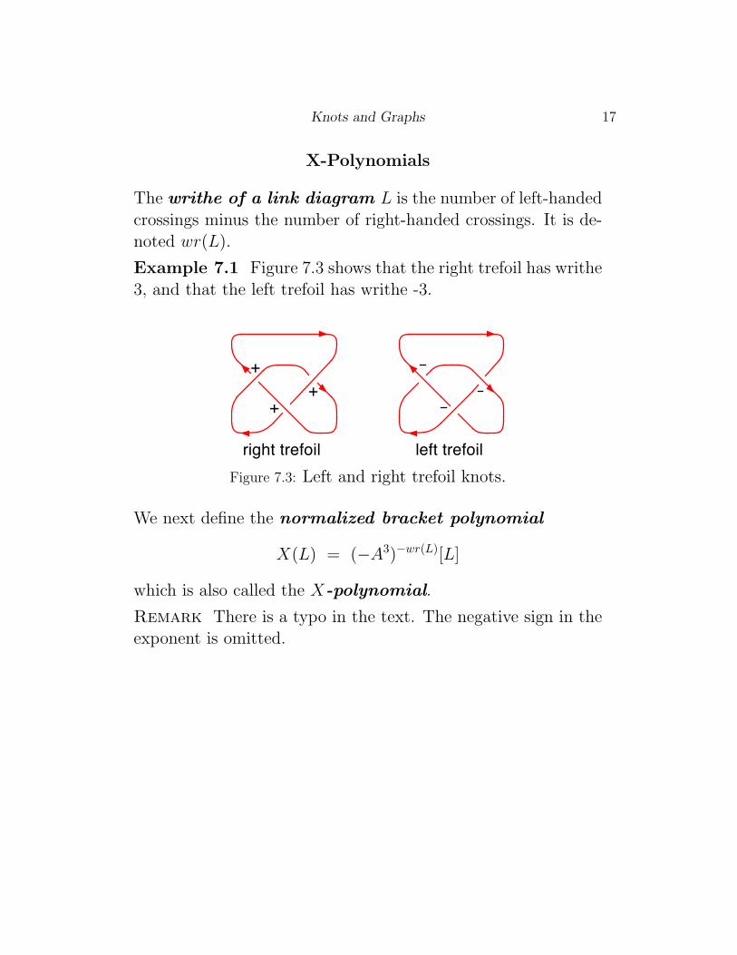
The writhe of a link diagram L is the number of left-handedcrossings minus the number of right-handed crossings. It is de-noted wr(L).

Example 7.1 Figure 7.3 shows that the right trefoil has writhe3, and that the left trefoil has writhe -3.

++

+

right trefoil left trefoilFigure 7.3: Left and right trefoil knots.

We next define the normalized bracket polynomial

X(L) = (−A3)−wr(L)[L]

which is also called the X-polynomial.

Remark There is a typo in the text. The negative sign in theexponent is omitted.

Knots and Graphs 18

Theorem 7.1 The X-polynomial is invariant under the threeReidemeister moves.

Proof for RM1

X(L ) = (-A3)-wr(L)-1[L ] = (-A3)-wr(L)(-A3)-1{A[L,O] + A-1[L ]}= (-A3)-wr(L)(-A-3){A(-A2-A-2)[L] + A-1[L]}= (-A3)-wr(L){(1+A-4)[L] - A-4[L]} = (-A3)-wr(L)[L] = X[L]

Proof for RM2

[L ] = A[L ] + A-1[L ]= A{A[L ]+A-1[L ]} + A-1{A[L ]+A-1[L ]}= (A2+A-2)[L ] + [L ] + (-A2-A-2)[L ]} = [L ]

X[L ] = X[L ]

Proof for RM2

[L ] =[L ]

A[L ] + A-1[L ]= A[L ] + A-1[L ] =

X[L ] = X[L ]

now apply invariance under RM2

Knots and Graphs 19

The Jones polynomial VL(t) of an oriented link is obtainedby substituting t1/4 for A in the X-polynomial XL(A). It is aLaurent polynomial, which means that negative degrees areallowed.

Trivial link with µ Components

Let Oµ be a trivial link with µ components. Then be applyinginduction, we obtain

[O1] = 1

[Om] =(−A2 − A−2) [Om−1]

∴ [Oµ] = (−1)µ−1 (A2 + A−2)µ−1

and we continue∴ X(Oµ) = (−1)µ−1 (

A2 + A−2)µ−1

∴ VOµ(t) = (−1)µ−1

(√t+

1√t

)µ−1

(7.1)

Knots and Graphs 20

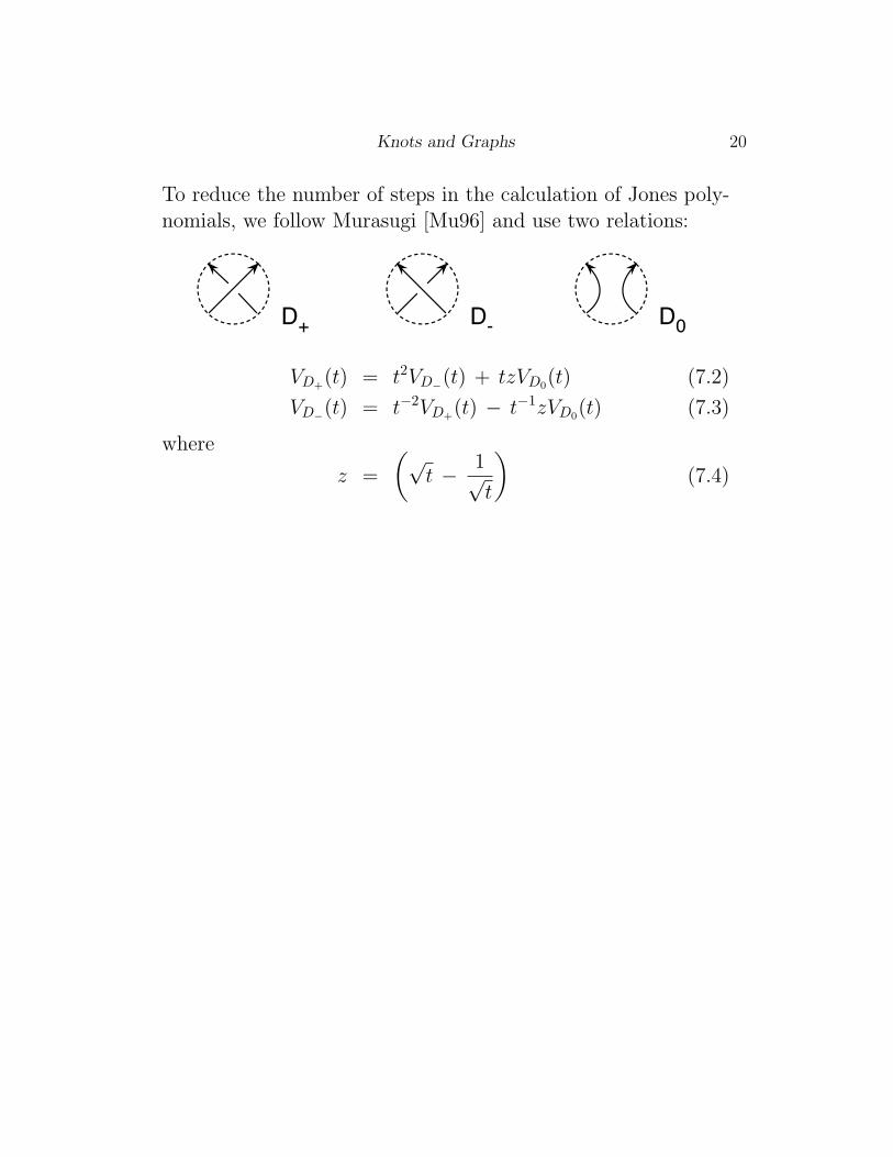
To reduce the number of steps in the calculation of Jones poly-nomials, we follow Murasugi [Mu96] and use two relations:

D0D-D+

VD+(t) = t2VD−(t) + tzVD0

(t) (7.2)

VD−(t) = t−2VD+(t) − t−1zVD0

(t) (7.3)

where

z =

(√t − 1√

t

)(7.4)

Knots and Graphs 21

The Hopf link

H0H-H

VH(t) = t2VH−(t) − tzVH0(t) by (7.2)

= t2(−1)

(√t+

1√t

)+ tz by (7.1)

= −t2.5 − t1.5 + t

(√t− 1√

t

)by (7.4)

= −t0.5 − t2.5

Exercise: Prove that if the orientation is changed on one (butnot both) of the components, then the Jones polynomial is

−t−0.5 − t−2.5

Knots and Graphs 22

Right trefoil knot

HT-T

VT (t) = t2VT−(t) + tzVH(t) by (7.2)

= t2 + t

(√t− 1√

t

) (−t0.5 − t2.5

)by (7.4), Hopf

= t+ t3 − t4

Left trefoil knot

HT+T

VT (t) = t−2VT+(t) − t−1zVH(t) by (7.3)

= t−2 − t−1(√

t− 1√t

) (−t−0.5 − t−2.5) by (7.4), Hopf*

= t−1 + t−3 − t−4

Knots and Graphs 23

References

[Ad94] C. C. Adams, The Knot Book, Amer. Math. Soc., 2004;original edn. Freeman, 1994.

[GrTu87] J. L. Gross and T. W. Tucker, Topological Graph The-ory, Dover, 2001; original edn. Wiley, 1987.

[Man04] V. Manturov, Knot Theory, CRC Press, 2004.

[Mu96] K. Murasugi, Knot Theory and Its Applications,Birkhauser, 1998; original edn., 1996.

[Rei32] K. Reidemeister, Knotentheorie, Chelsea, 1948; originaledn. Springer, 1932.