CS 59000 Statistical Machine learning Lecture 24 Yuan (Alan) Qi Purdue CS Nov. 20 2008.
36
CS 59000 Statistical Machine learning Lecture 24 Yuan (Alan) Qi Purdue CS Nov. 20 2008
-
Upload
magdalene-arnold -
Category
Documents
-
view
218 -
download
0
Transcript of CS 59000 Statistical Machine learning Lecture 24 Yuan (Alan) Qi Purdue CS Nov. 20 2008.

CS 59000 Statistical Machine learningLecture 24
Yuan (Alan) QiPurdue CS
Nov. 20 2008
Outline
• Review of K-medoids, Mixture of Gaussians, Expectation Maximization (EM), Alternative view of EM
• Hidden Markvo Models, forward-backward algorithm, EM for learning HMM parameters, Viterbi Algorithm, Linear state space models, Kalman filtering and smoothing

K-medoids Algorithm

Mixture of Gaussians
Mixture of Gaussians:
Introduce latent variables:
Marginal distribution:
Conditional Probability
Responsibility that component k takes for explaining the observation.
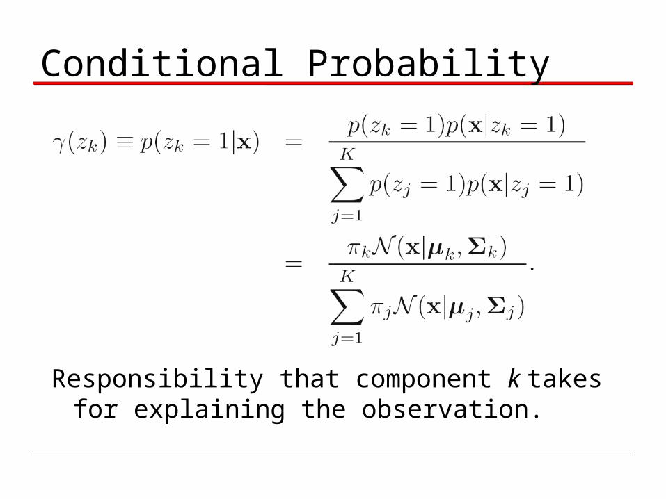
Maximum Likelihood
Maximize the log likelihood function
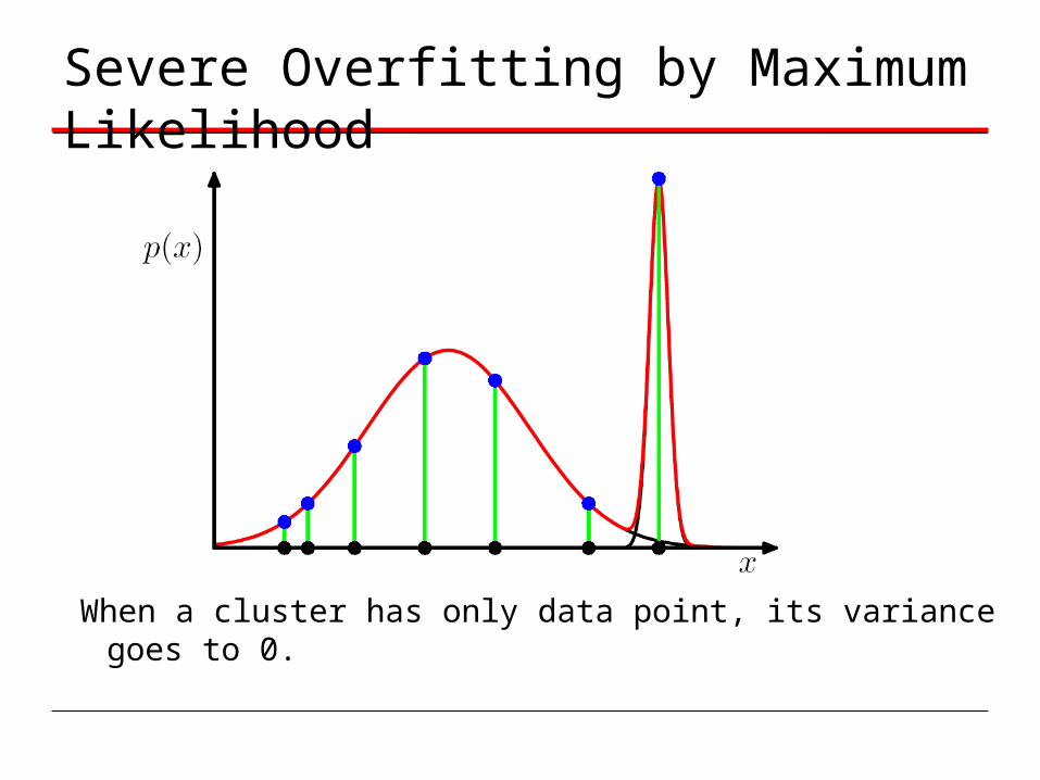
Severe Overfitting by Maximum Likelihood
When a cluster has only data point, its variance goes to 0.

Maximum Likelihood Conditions (1)
Setting the derivatives of to zero:
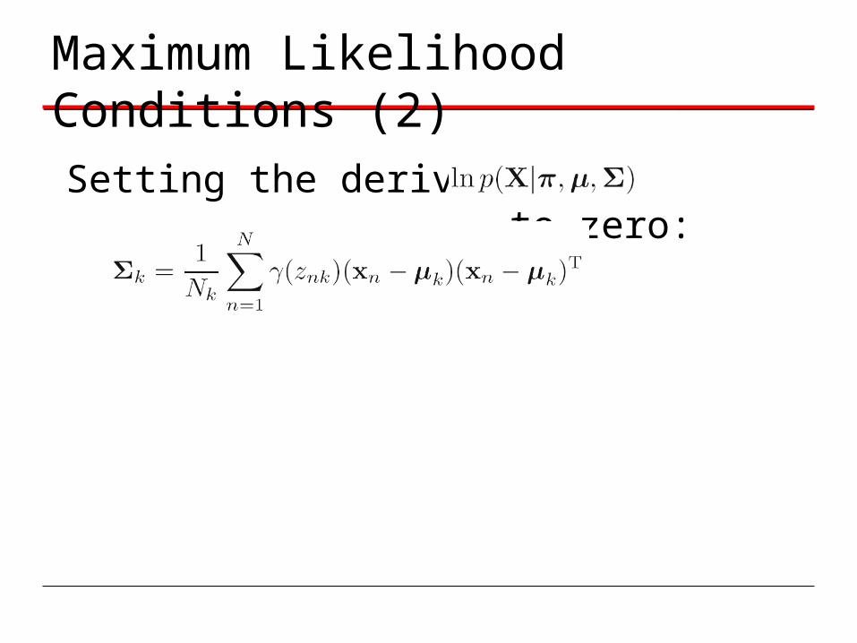
Maximum Likelihood Conditions (2)
Setting the derivative of to zero:

Maximum Likelihood Conditions (3)
Lagrange function:
Setting its derivative to zero and use the normalization constraint, we obtain:

Expectation Maximization for Mixture Gaussians
Although the previous conditions do not provide closed-form conditions, we can use them to construct iterative updates:
E step: Compute responsibilities .M step: Compute new mean , variance ,
and mixing coefficients .Loop over E and M steps until the log
likelihood stops to increase.
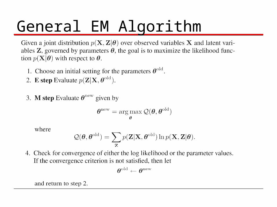
General EM Algorithm

EM and Jensen Inequality
Goal: maximize
Define:
We haveFrom Jesen’s Inequality, we see is a lower
bound of .

Lower Bound
is a functional of the distribution .
Since and , is a lower bound of the log likelihood
function . (Another way to see the lower bound without using Jensen’s inequality)

Lower Bound Perspective of EM
• Expectation Step:Maximizing the functional lower bound over the distribution .
• Maximization Step:Maximizing the lower bound over the parameters .

Illustration of EM Updates
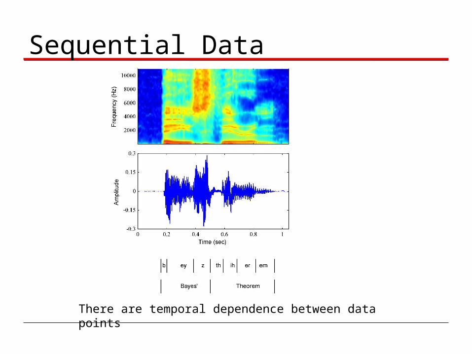
Sequential Data
There are temporal dependence between data points
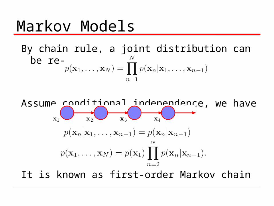
Markov ModelsBy chain rule, a joint distribution can be re-written as:
Assume conditional independence, we have
It is known as first-order Markov chain
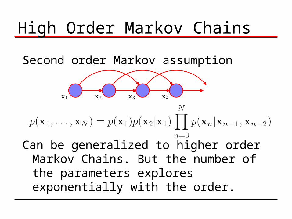
High Order Markov Chains
Second order Markov assumption
Can be generalized to higher order Markov Chains. But the number of the parameters explores exponentially with the order.
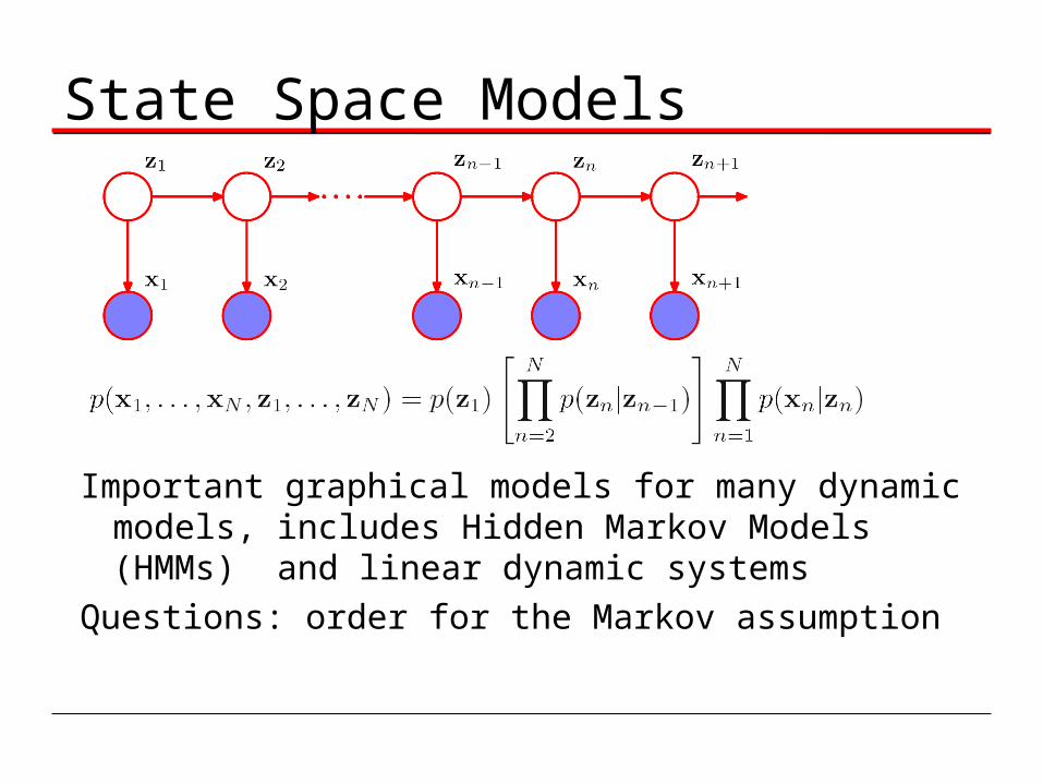
State Space Models
Important graphical models for many dynamic models, includes Hidden Markov Models (HMMs) and linear dynamic systems
Questions: order for the Markov assumption
Hidden Markov Models
Many applications, e.g., speech recognition, natural language processing, handwriting recognition, bio-sequence analysis

From Mixture Models to HMMs
By turning a mixture Model into a dynamic model, we obtain the HMM.
Let model the dependence between two consecutive latent variables by a transition probability:

HMMs
Prior on initial latent variable:
Emission probabilities:
Joint distribution:

Samples from HMM
(a) Contours of constant probability density for the emission distributions corresponding to each of the three states of the latent variable. (b) A sample of 50 points drawn from the hidden Markov model, with lines connecting the successive observations.

Inference: Forward-backward Algorithm
Goal: compute marginals for latent variables.Forward-backward Algorithm: exact inference
as special case of sum-product algorithm on the HMM.
Factor graph representation (grouping emission density and transition probability in one factor at a time):

Forward-backward Algorithm as Message Passing Method (1)
Forward messages:

Forward-backward Algorithm as Message Passing Method (2)
Backward messages (Q: how to compute it?):
The messages actually involves X
Similarly, we can compute the following (Q: why)

Rescaling to Avoid OverflowingWhen a sequence is long, the forward message will become to
small to be represented by the dynamic range of the computer. We redefine the forward message
asSimilarly, we re-define the backward message
asThen, we can compute
See detailed derivation in textbook

Viterbi Algorithm
Viterbi Algorithm: • Finding the most probable sequence of
states• Special case of sum-product algorithm on
HMM.What if we want to find the most probable
individual states?
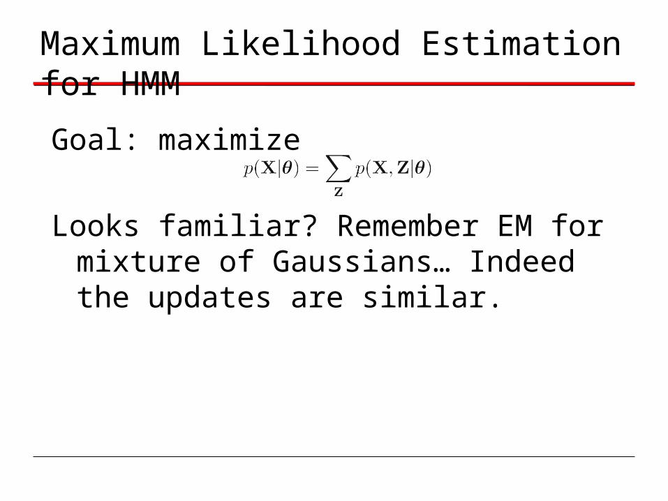
Maximum Likelihood Estimation for HMM
Goal: maximize
Looks familiar? Remember EM for mixture of Gaussians… Indeed the updates are similar.
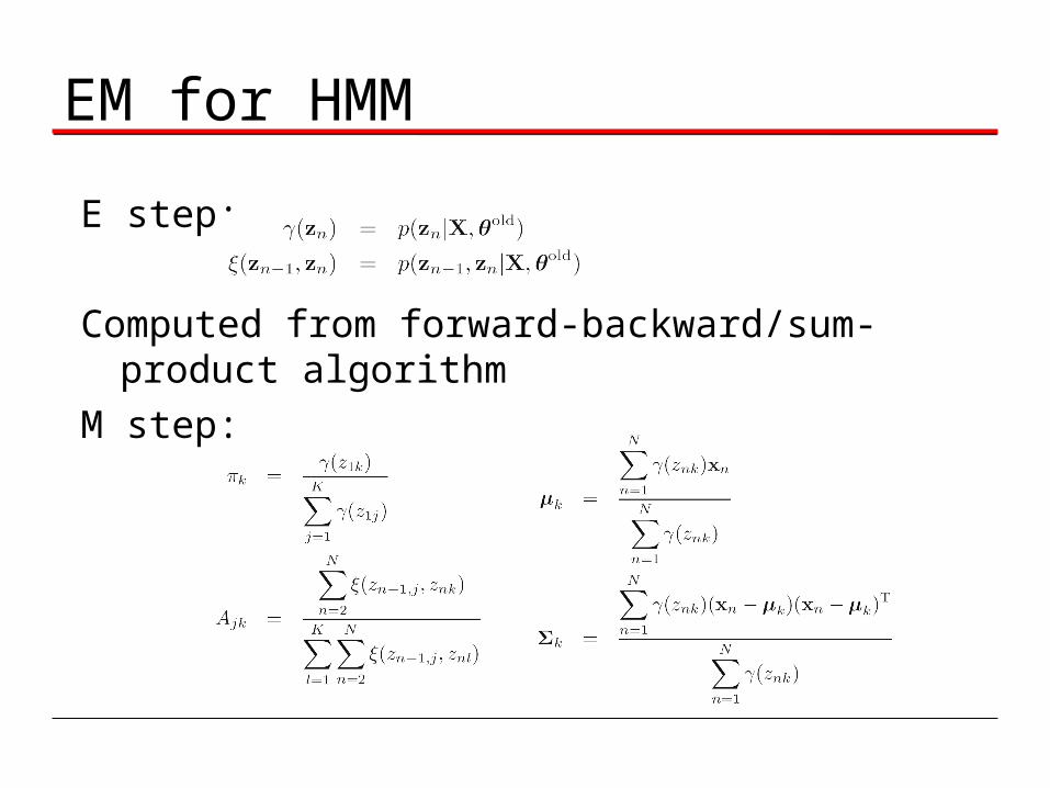
EM for HMM
E step:
Computed from forward-backward/sum-product algorithm
M step:
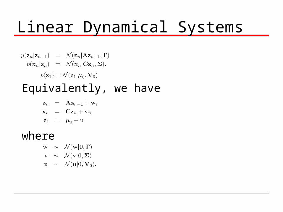
Linear Dynamical Systems
Equivalently, we have
where

Kalman Filtering and Smoothing
Inference on linear Gaussian systems.Kalman filtering: sequentially update scaled
forward message: Kalman smoothing: sequentially update state
beliefs based on scaled forward and backward messages:
Learning in LDS
EM again…
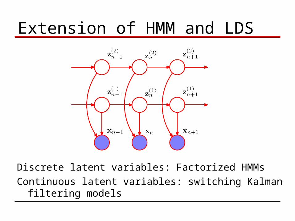
Extension of HMM and LDS
Discrete latent variables: Factorized HMMsContinuous latent variables: switching Kalman filtering models