CS 526: Computer Graphics II University of Illinois at Chicago “Probabilistic Surfaces: Point...

CS 526: Computer Graphics II University of Illinois at Chicago

“Probabilistic Surfaces:Point Based Primitives

to Show Surface Uncertainty”

Authors: Gevorg Grigoryan and Penny Rheingans

Presented by: Allan Spale, Spring 2004


Uncertainty Is Inevitable

• Technical fields have measurements with an amount of uncertainty– Example: 25 mm +/- 2 mm

• Visualizations require a merging of the main data being displayed in addition to the uncertainty values– Especially crucial when decision-making must

be done by users of the visualization


Traditional Uncertainty Visualization

• Examples– Vertical bars on bar graphs– Probability density curves and surfaces– Adjacent displays of data and its uncertainty

• Problem– Does not scale well to multidimensional data

1 2


Uncertainty Visualization:Discrete Points

• Examples– Glyphs [12,16]; sonification (sound used to

convey data) [7, 9, 11]; discrete point distribution [14]; procedural annotation [2]

• Advantage– Useful sampling

• Disadvantage– Using discrete points limits its application to

continuous domains


Uncertainty Visualization:Pseudo-coloring

• Example– Coloring a mountain range to show the likelihood of an

avalanche or mud slide

• Advantage– Uncertainty displayed continuously

• Disadvantages– Uncertainty relates to a variable, not to a single point

or group of points– Disconnect between uncertainty and geometry

• Further reading in [17]


Uncertainty Visualization:Geometry Modification

• Examples– Fat surfaces (surfaces with thickness) [1, 12]– Displaced/perturbed geometry [10, 12]; – Animation [4], – IFS (iterated function system) fractal interpolation [18]

• Advantages– Fat surfaces: illustrate potential range of data point locations– Animation: easy to detect uncertainty– Fractals: good for introducing geometric variability

• Disadvantages– Animation: not printable to paper, motion distracts from other

variables


Uncertainty Visualization:Probabilistic Surfaces

• Application– MRI of brain showing probabilities of cancerous

tumor boundaries

• Requirements to be successful– Information about both surface geometry and

regional uncertainty– Intuitive and not distracting– Display of other variables in addition to

uncertainty


Tumor Growth Model:General Information

• Gompertz model [15]: V(t) = V(0) exp( A/B ( 1 – exp( -Bt ) ) )

– Parameters• V(0): initial volume of tumor at time t = 0• A, B: tumor growth parameters

– Trends

• t (as t approaches infinity):

– A/B = final tumor size– B = rate of initial growth

– Used to build a large tumor from small tumors dispersed in a region


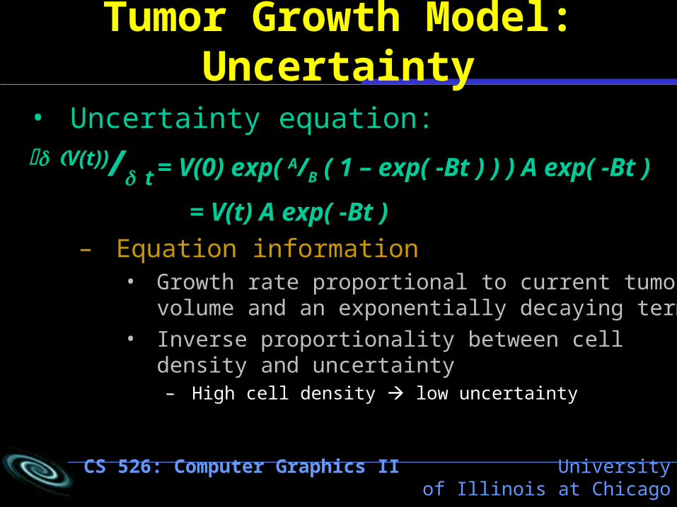
Tumor Growth Model:Uncertainty

• Uncertainty equation:V(t))/t = V(0) exp( A/B ( 1 – exp( -Bt ) ) ) A exp( -Bt )

= V(t) A exp( -Bt )

– Equation information• Growth rate proportional to current tumor volume

and an exponentially decaying term• Inverse proportionality between cell density and

uncertainty – High cell density low uncertainty


Tumor Growth Model:Uncertainty

• Uncertainty equation: V(t))/t = V(0) exp( A/B ( 1 – exp( -Bt ) ) ) A exp( -Bt )

= V(t) A exp( -Bt )

– Equation information

• t (as t approaches infinity):

– Uncertainty 0– Growth rate 0 – Tumor reaches a constant volume


Tumor Growth Model:Metastasis

• Description– As cancer develops, cells separate from tumor– Cells travel in blood vessels and settle in a new

place

• Parameter in the growth model– At an increasing time interval t, tumor size

increases• At some size threshold, metastasis occurs• New tumor center created at a random distance from

the origin in the direction of the blood vessel flow

– Output as age along with an uncertainty value


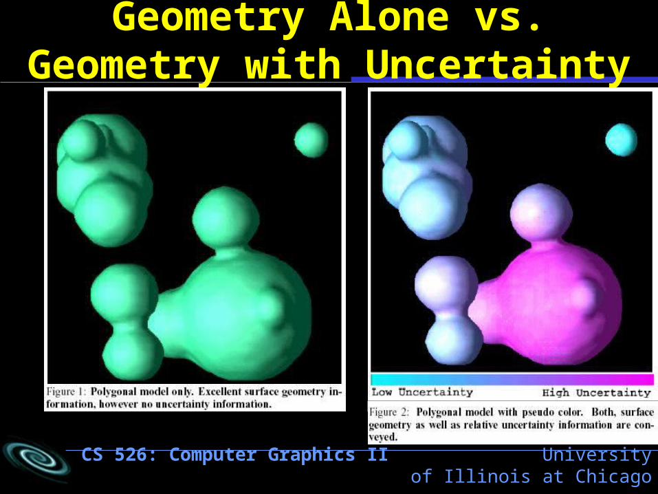
Geometry Alone vs.Geometry with Uncertainty


Approach toUncertainty Points

• For each surface point, displace it along the surface normal of the point– Point displacement is proportional to the point’s

uncertainty value

• Reasons to use points instead of polygons– Levoy & Whitted (1985) pioneered the use of

points as display primitives (paper reference [8])– Increasing scene complexity reduces algorithm

design complexity– Do not have to consider surfaces at polygons


Improved Approach toUncertainty Points

• Transparency is appropriate for displaying uncertainty

• High uncertainty high transparency

• Result– Highly uncertain regions will contain points with

blurriness and large displacements


Implementation:Initialization

1. Read in surface and uncertainty information (polygon mesh with uncertainty data at vertices – uncertainty values between 0 and 1)

• Note: The text for all implementation steps are directly quoted from the paper.

Surface Info Uncertainty Info

Uncertainty Transform

DisplayPrimitives

Points Polygons

PolygonModel

Y


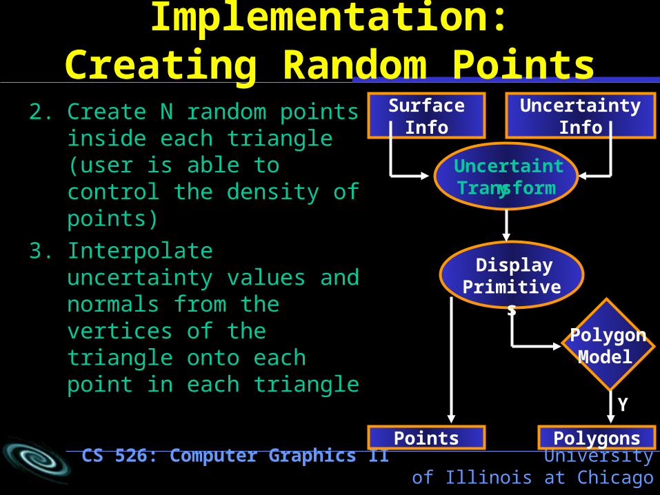
Implementation:Creating Random Points

2. Create N random points inside each triangle (user is able to control the density of points)

3. Interpolate uncertainty values and normals from the vertices of the triangle onto each point in each triangle



DisplayPrimitives

Points Polygons

PolygonModel

Y


Implementation:Calculating Displacement

4. For each point P do…5. Calculate the

displacement:disp = rand( )

* ( uncertainty at P )a * ( scale factor )

• rand() returns a random number between the values of 0 and 1

• a and scale factor are controlled by the user



DisplayPrimitives

Points Polygons

PolygonModel

Y


Implementation: Point Displacement & Transparency

4. For each point P do…6. Displace P in the

direction of the normal at P

7. Calculate the transparency, alpha:alpha = 1 –

( uncertainty at P )b

• b is controlled by the user



DisplayPrimitives

Points Polygons

PolygonModel

Y


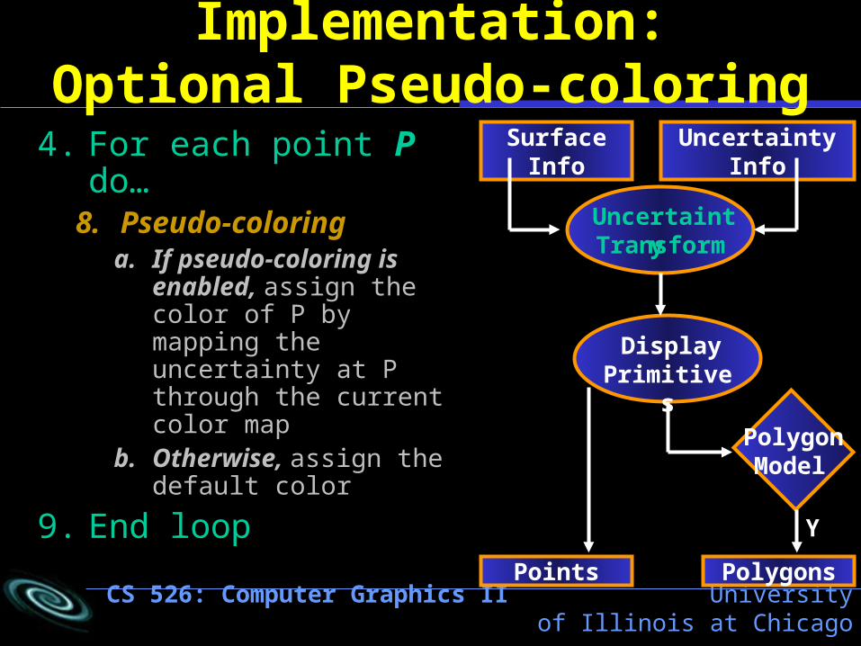
Implementation:Optional Pseudo-coloring

4. For each point P do…8. Pseudo-coloring

a. If pseudo-coloring is enabled, assign the color of P by mapping the uncertainty at P through the current color map

b. Otherwise, assign the default color

9. End loop



DisplayPrimitives

Points Polygons

PolygonModel

Y


Implementation:Displaying the Primitives

10. Display all points

11. Polygons12. If polygonal model

usage is enabled, display all the polygons



DisplayPrimitives

Points Polygons

PolygonModel

Y


Implementation: Results

• Simplest version– Certain and uncertain

areas are clearly displayed– The uncertainty area of the

tumor boundary is clearly defined

• Size of region proportional to level of uncertainty

– Best suited for interactive display

– Disadvantage• Artifacts; difficulty making

dense areas smooth

Uncertain Region

Certain Region


Enhancement:Adding Polygonal Rendering

• Improving computational efficiency– Use point rendering for

uncertain areas– Use polygonal rendering

for certain areas regardless of its point density

• Advantages– Well-defined low

uncertainty areas– More pleasing to view

and more informative

Uncertain Region

Certain Region


Enhancement:Adjusting Transparency

• Adjust transparency according to uncertainty level using the equation: = 1.0 – err c

• err : uncertainty value scaled from 0 to 1• c : rate that

transparency increases with uncertainty; constant value

Uncertain Region

Certain Region


Reviewing Uncertainty Visualization Requirements

• Informative– Polygonal (certainty) and

point (uncertainty) rendering

• Intuitive/not distracting– Transparency value =

uncertainty value

• Additional information– Inclusion of tumor age

• Correlation between tumor age and uncertainty

• Seemingly contradictory items (blue, green arrows) remain valid for Equation 2

Young tumor; high uncertainty

Old tumor; high uncertainty

Young tumor; low uncertainty


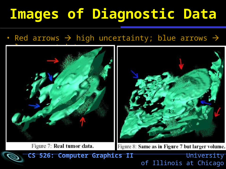
Application to Diagnostic Data

• Datasets of CAT scan of human kidney tumors• Creation of the visualization

– Input• Each point is in 3-D with a density value

– Output• Geometry: used isovalue of tumor density to create the

isosurface volume• Certainty: at the tumor surface, used inverse density gradient

– Results• High density gradient sharp border• Low density gradient “fuzzy” border• Certainty data coexists with geometry data• Scalable to larger datasets


Images of Diagnostic Data

• Red arrows high uncertainty; blue arrows low uncertainty


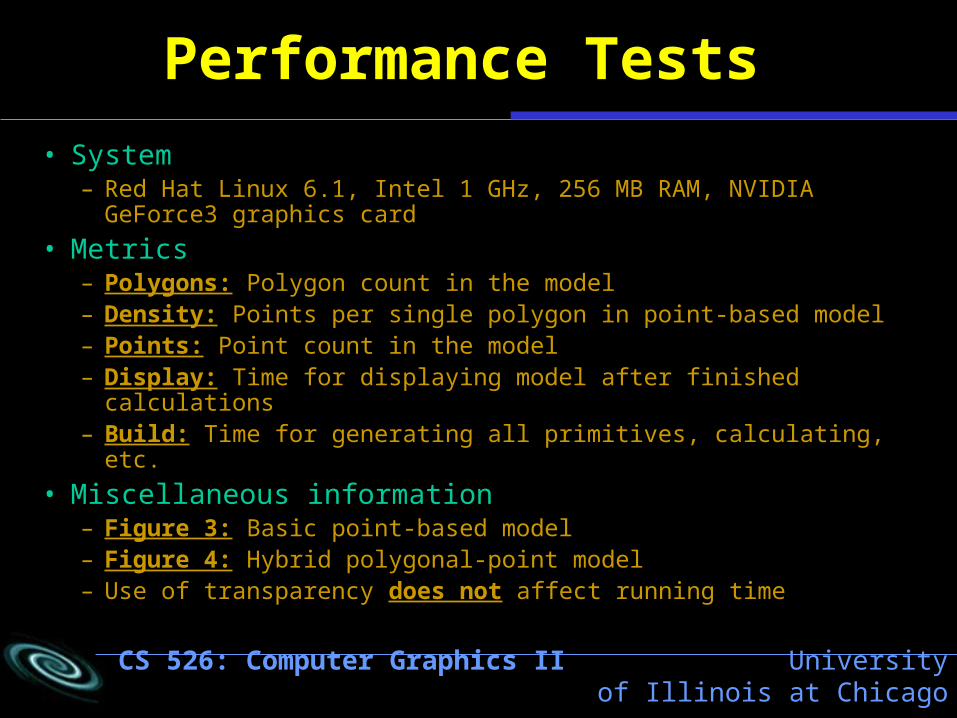
Performance Tests

• System– Red Hat Linux 6.1, Intel 1 GHz, 256 MB RAM, NVIDIA GeForce3

graphics card

• Metrics– Polygons: Polygon count in the model– Density: Points per single polygon in point-based model– Points: Point count in the model– Display: Time for displaying model after finished calculations– Build: Time for generating all primitives, calculating, etc.

• Miscellaneous information– Figure 3: Basic point-based model– Figure 4: Hybrid polygonal-point model– Use of transparency does not affect running time


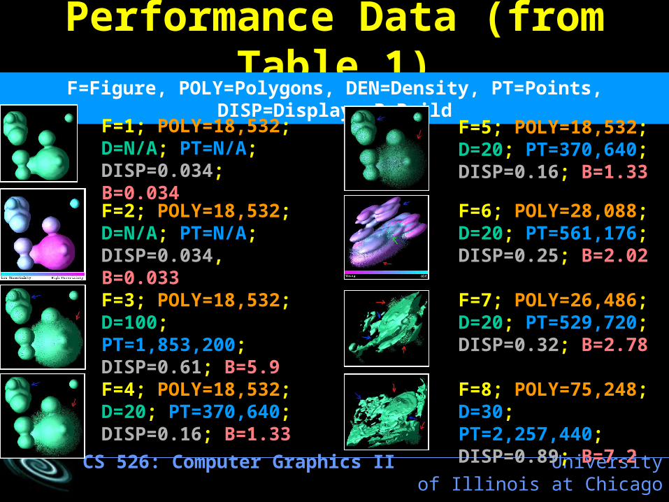
Performance Data (from Table 1)F=Figure, POLY=Polygons, DEN=Density, PT=Points, DISP=Display, B=Build

F=1; POLY=18,532; D=N/A; PT=N/A; DISP=0.034; B=0.034

F=2; POLY=18,532; D=N/A; PT=N/A; DISP=0.034, B=0.033

F=3; POLY=18,532; D=100; PT=1,853,200; DISP=0.61; B=5.9

F=4; POLY=18,532; D=20; PT=370,640; DISP=0.16; B=1.33

F=8; POLY=75,248; D=30; PT=2,257,440; DISP=0.89; B=7.2

F=7; POLY=26,486; D=20; PT=529,720; DISP=0.32; B=2.78

F=6; POLY=28,088; D=20; PT=561,176; DISP=0.25; B=2.02

F=5; POLY=18,532; D=20; PT=370,640; DISP=0.16; B=1.33


Summary & Future Work

• Point-based model for uncertainty visualization is successful– Geometry and uncertainty data can coexist– Adding polygonal mesh increases run-time

efficiency– Use of transparency creates an intuitive model

• Future improvements– More parameters to display uncertainty

• Specular coefficient• Refractive index


Thanks for listening


Paper References[1] R.E. Barnhill, K. Opitz, and H. Pottmann. Fat surfaces: A trivariate approach to triangle-based interpolation on

surfaces. Computer Aided Geometric Design, 9(5):365–378, 1992.

[2] Andrej Cedilnik and Penny Rheingans. Procedural annotation of uncertain information. In Proceedings of IEEE Visualization ’00, pages 77–84. IEEE, 2000.

[3] Baoquan Chen and Minh Xuan Nguyen. POP: A hybrid point and polygon rendering system for large data. In Proceedings of Visualization 2001, pages 45–52. IEEE, 2001.

[4] C.R. Ehlschlaeger, A.M. Shortridge, and M.F. Goodchild. Visualizing spatial data uncertainty using animation. Computers in GeoSciences, 23(4):387–395, 1997.

[5] Markus Gross. Are points the better graphics primitives? Computer Graphics Forum, 20(3), 2001.

[6] A.R. Kansal, S. Torquato, G.R.IV Harsh, E.A. Chiocca, and T.S. Deisboeck. Simulated brain tumor growth dynamics using a three-dimensional cellular automaton. Journal of Theoretical Biology, 203:367–382, 2000.

[7] Gregory Kramer. Auditory Display, Sonification, Audification, and Auditory Interfaces, pages 1–78. Addison-Wesley, 1994.

[8] Marc Levoy and Turner Whitted. The use of points as a display primitive. Technical Report 85-022, University of North Carolina at Chapel Hill, January 1985.

[9] S. K. Lodha, C. M. Wilson, and R. E. Sheehan. LISTEN: sounding uncertainty visualization. In Proceedings of Visualization 96, pages 189–195. IEEE, 1996.


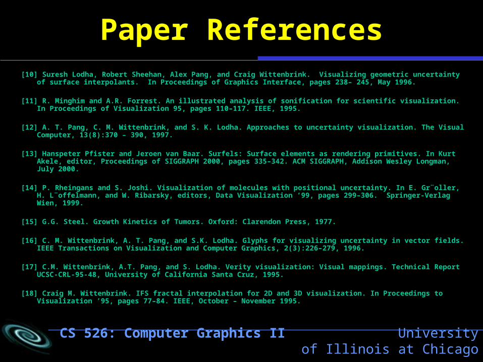
Paper References[10] Suresh Lodha, Robert Sheehan, Alex Pang, and Craig Wittenbrink. Visualizing geometric uncertainty of surface

interpolants. In Proceedings of Graphics Interface, pages 238– 245, May 1996.

[11] R. Minghim and A.R. Forrest. An illustrated analysis of sonification for scientific visualization. In Proceedings of Visualization 95, pages 110–117. IEEE, 1995.

[12] A. T. Pang, C. M. Wittenbrink, and S. K. Lodha. Approaches to uncertainty visualization. The Visual Computer, 13(8):370 – 390, 1997.

[13] Hanspeter Pfister and Jeroen van Baar. Surfels: Surface elements as rendering primitives. In Kurt Akele, editor, Proceedings of SIGGRAPH 2000, pages 335–342. ACM SIGGRAPH, Addison Wesley Longman, July 2000.

[14] P. Rheingans and S. Joshi. Visualization of molecules with positional uncertainty. In E. Gr¨oller, H. L¨offelmann, and W. Ribarsky, editors, Data Visualization ’99, pages 299–306. Springer-Verlag Wien, 1999.

[15] G.G. Steel. Growth Kinetics of Tumors. Oxford: Clarendon Press, 1977.

[16] C. M. Wittenbrink, A. T. Pang, and S.K. Lodha. Glyphs for visualizing uncertainty in vector fields. IEEE Transactions on Visualization and Computer Graphics, 2(3):226–279, 1996.

[17] C.M. Wittenbrink, A.T. Pang, and S. Lodha. Verity visualization: Visual mappings. Technical Report UCSC-CRL-95-48, University of California Santa Cruz, 1995.

[18] Craig M. Wittenbrink. IFS fractal interpolation for 2D and 3D visualization. In Proceedings to Visualization ’95, pages 77–84. IEEE, October – November 1995.


Credits and References

• Non-paper sources• Microsoft Excel 2000, Help: “Error bars in charts”• Microsoft Excel 2000, Help: “Examples of Chart Types: XY

Scatter”• Paper sources

• All images labeled “figure”• Internet

• IFS: http://www.cse.ucsc.edu/research/slvg/ifs.html• Fat Surfaces: http://www.ticam.utexas.edu/reports/1999/9908.pdf


Questions and Comments

CS 526: Computer Graphics II University of Illinois at Chicago “Probabilistic Surfaces: Point...

Documents

Transcript of CS 526: Computer Graphics II University of Illinois at Chicago “Probabilistic Surfaces: Point...