Bruce Bobick - Watercolor Artist · Author: Bruce Bobick Created Date: 4/13/2009 6:11:41 PM

Tracking CS 4495 Computer Vision – A. Bobick
Aaron Bobick School of Interactive Computing
CS 4495 Computer Vision Tracking 1- Kalman,Gaussian

Tracking CS 4495 Computer Vision – A. Bobick
Administrivia • PS5 – will be out this Thurs
• Due Sun Nov 10th 11:55pm
• Calendar (tentative) done for the year • PS6: 11/14, due 11/24 PS7: 11/26, due 12/5 • EXAM: Tues before Thanksgiving. Covers concepts and basics • So no final on Dec 12….

Tracking CS 4495 Computer Vision – A. Bobick
Tracking • Slides “adapted” from Kristen Grauman, Deva Ramanan,
but mostly from Svetlana Lazebnik

Tracking CS 4495 Computer Vision – A. Bobick
Some examples • Older examples:
• State of the art: http://www.youtube.com/watch?v=InqV34BcheM

Tracking CS 4495 Computer Vision – A. Bobick
Feature tracking • So far, we have only considered optical flow estimation in
a pair of images • If we have more than two images, we can compute the
optical flow from each frame to the next • Given a point in the first image, we can in principle
reconstruct its path by simply “following the arrows”

Tracking CS 4495 Computer Vision – A. Bobick
Tracking challenges • Ambiguity of optical flow
• Find good features to track
• Large motions • Discrete search instead of Lucas-Kanade
• Changes in shape, orientation, color • Allow some matching flexibility
• Occlusions, disocclusions • Need mechanism for deleting, adding new features
• Drift – errors may accumulate over time
• Need to know when to terminate a track

Tracking CS 4495 Computer Vision – A. Bobick
Handling large displacements • Define a small area around a pixel as the template • Match the template against each pixel within a search
area in next image – just like stereo matching! • Use a match measure such as SSD or correlation • After finding the best discrete location, can use Lucas-
Kanade to get sub-pixel estimate (think of the template as the coarse level of the pyramid).

Tracking CS 4495 Computer Vision – A. Bobick
Tracking over many frames • Select features in first frame • For each frame:
• Update positions of tracked features • Discrete search or Lucas-Kanade
• Start new tracks if needed • Terminate inconsistent tracks
• Compute similarity with corresponding feature in the previous frame or in the first frame where it’s visible
• This is done by many companies and systems – often ad hoc rules tailored to the context.
Tracking CS 4495 Computer Vision – A. Bobick
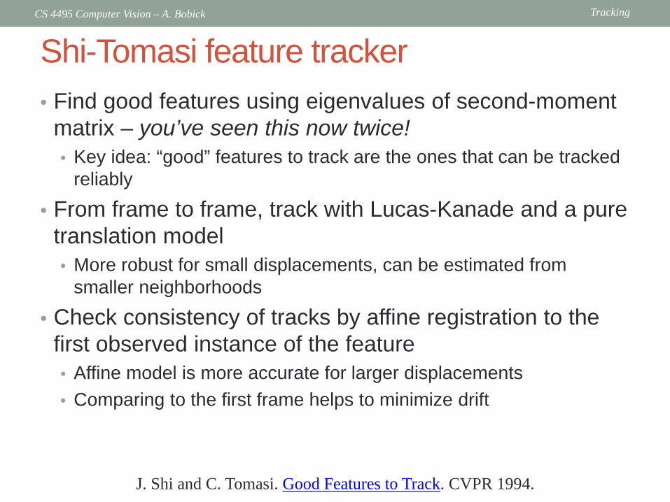
Shi-Tomasi feature tracker • Find good features using eigenvalues of second-moment
matrix – you’ve seen this now twice! • Key idea: “good” features to track are the ones that can be tracked
reliably
• From frame to frame, track with Lucas-Kanade and a pure translation model • More robust for small displacements, can be estimated from
smaller neighborhoods
• Check consistency of tracks by affine registration to the first observed instance of the feature • Affine model is more accurate for larger displacements • Comparing to the first frame helps to minimize drift
J. Shi and C. Tomasi. Good Features to Track. CVPR 1994.

Tracking CS 4495 Computer Vision – A. Bobick
Tracking example
J. Shi and C. Tomasi. Good Features to Track. CVPR 1994.

Tracking CS 4495 Computer Vision – A. Bobick
Tracking with dynamics • Key idea: Given a model of expected motion, predict
where objects will occur in next frame, even before seeing the image • Restrict search for the object • Improved estimates since measurement noise is reduced by
trajectory smoothness

Tracking CS 4495 Computer Vision – A. Bobick
Tracking as inference • The hidden state consists of the true parameters we care
about, denoted X.
• The measurement is our noisy observation that results from the underlying state, denoted Y.
• At each time step, state changes (from Xt-1 to Xt ) and we get a new observation Yt.
• Our goal: recover most likely state Xt given • All observations seen so far. • Knowledge about dynamics of state transitions.

Tracking CS 4495 Computer Vision – A. Bobick
old belief
measurement
Belief: prediction
Corrected prediction
Belief: prediction
Time t Time t+1
Tracking as inference: intuition

Tracking CS 4495 Computer Vision – A. Bobick
Steps of tracking • Prediction: What is the next state of the object given past
measurements? ( )1100 ,, −− == ttt yYyYXP

Tracking CS 4495 Computer Vision – A. Bobick
Steps of tracking • Prediction: What is the next state of the object given past
measurements?
• Correction: Compute an updated estimate of the state from prediction and measurements
( )1100 ,, −− == ttt yYyYXP
( )ttttt yYyYyYXP === −− ,,, 1100

Tracking CS 4495 Computer Vision – A. Bobick
Steps of tracking • Prediction: What is the next state of the object given past
measurements?
• Correction: Compute an updated estimate of the state from prediction and measurements (posterior)
• Tracking can be seen as the process of propagating the posterior distribution of state given measurements across time
( )1100 ,, −− == ttt yYyYXP
( )ttttt yYyYyYXP === −− ,,, 1100

Tracking CS 4495 Computer Vision – A. Bobick
Simplifying assumptions • Only the immediate past matters
( ) ( )110 ,, −− = tttt XXPXXXP
dynamics model

Tracking CS 4495 Computer Vision – A. Bobick
Simplifying assumptions • Only the immediate past matters
• Measurements depend only on the current state
( ) ( )tttttt XYPXYXYXYP =−− ,,,, 1100
( ) ( )110 ,, −− = tttt XXPXXXP
observation model
dynamics model

Tracking CS 4495 Computer Vision – A. Bobick
Simplifying assumptions • Only the immediate past matters
• Measurements depend only on the current state
( ) ( )tttttt XYPXYXYXYP =−− ,,,, 1100
( ) ( )110 ,, −− = tttt XXPXXXP
observation model
dynamics model
X1 X2
Y1 Y2
Xt
Yt
… Hmmm….
Tracking CS 4495 Computer Vision – A. Bobick
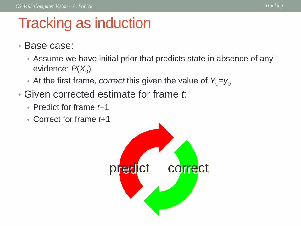
Tracking as induction • Base case:
• Assume we have initial prior that predicts state in absence of any evidence: P(X0)
• At the first frame, correct this given the value of Y0=y0
• Given corrected estimate for frame t: • Predict for frame t+1 • Correct for frame t+1
predict correct

Tracking CS 4495 Computer Vision – A. Bobick
Tracking as induction • Base case:
• Assume we have initial prior that predicts state in absence of any evidence: P(X0)
• At the first frame, correct this given the value of Y0=y0
)()|()(
)()|()|( 0000
000000 XPXyP
yPXPXyPyYXP ∝==

Tracking CS 4495 Computer Vision – A. Bobick
Prediction • Prediction involves guessing
given
( )10 ,, −tt yyXP
( )101 ,, −− tt yyXP
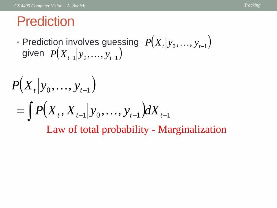
Tracking CS 4495 Computer Vision – A. Bobick
Prediction • Prediction involves guessing
given
( )10 ,, −tt yyXP
( )101 ,, −− tt yyXP
( )( ) ( )( ) ( ) 11011
1101101
1101
,,||
,,|,,,|
,,,
−−−−
−−−−−
−−−
∫∫∫
=
=
=
ttttt
tttttt
tttt
dXyyXPXXP
dXyyXPyyXXP
dXyyXXP
( )10 ,, −tt yyXP
Law of total probability - Marginalization

Tracking CS 4495 Computer Vision – A. Bobick
Prediction • Prediction involves guessing
given
( )10 ,, −tt yyXP
( )101 ,, −− tt yyXP
( )( ) ( )( ) ( ) 11011
1101101
1101
,,||
,,|,,,|
,,,
−−−−
−−−−−
−−−
∫∫∫
=
=
=
ttttt
tttttt
tttt
dXyyXPXXP
dXyyXPyyXXP
dXyyXXP
( )10 ,, −tt yyXP
Conditioning on Xt–1

Tracking CS 4495 Computer Vision – A. Bobick
Prediction • Prediction involves guessing
given
( )10 ,, −tt yyXP
( )101 ,, −− tt yyXP
( )( ) ( )( ) ( ) 11011
1101101
1101
,,||
,,|,,,|
,,,
−−−−
−−−−−
−−−
∫∫∫
=
=
=
ttttt
tttttt
tttt
dXyyXPXXP
dXyyXPyyXXP
dXyyXXP
( )10 ,, −tt yyXP
Independence assumption
Tracking CS 4495 Computer Vision – A. Bobick
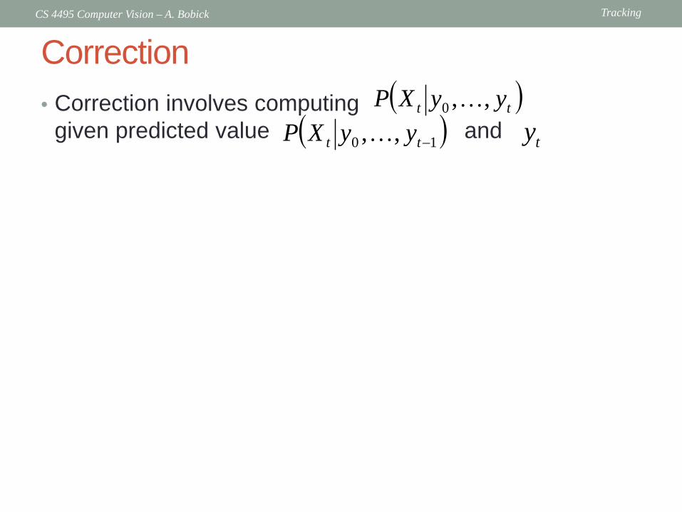
Correction • Correction involves computing
given predicted value and
( )tt yyXP ,,0
( )10 ,, −tt yyXP ty

Tracking CS 4495 Computer Vision – A. Bobick
Correction • Correction involves computing
given predicted value and
( )10 ,, −tt yyXP
( )tt yyXP ,,0
( ) ( )( )
( ) ( )( )
( ) ( )( ) ( )∫ −
−
−
−
−
−−
=
=
=
ttttt
tttt
tt
tttt
tt
ttttt
dXyyXPXyPyyXPXyP
yyyPyyXPXyPyyyP
yyXPyyXyP
10
10
10
10
10
1010
,,||,,||
,,|,,||,,|
,,|,,,|
( )tt yyXP ,,0
Bayes rule
ty

Tracking CS 4495 Computer Vision – A. Bobick
Correction • Correction involves computing
given predicted value and
( )tt yyXP ,,0
( ) ( )( )
( ) ( )( )
( ) ( )( ) ( )∫ −
−
−
−
−
−−
=
=
=
ttttt
tttt
tt
tttt
tt
ttttt
dXyyXPXyPyyXPXyP
yyyPyyXPXyPyyyP
yyXPyyXyP
10
10
10
10
10
1010
,,||,,||
,,|,,||,,|
,,|,,,|
( )10 ,, −tt yyXP
( )tt yyXP ,,0
Independence assumption (observation yt depends only on state Xt)
ty

Tracking CS 4495 Computer Vision – A. Bobick
Correction • Correction involves computing
given predicted value and ( )tt yyXP ,,0
( ) ( )( )
( ) ( )( )
( ) ( )( ) ( )∫ −
−
−
−
−
−−
=
=
=
ttttt
tttt
tt
tttt
tt
ttttt
dXyyXPXyPyyXPXyP
yyyPyyXPXyPyyyP
yyXPyyXyP
10
10
10
10
10
1010
,,||,,||
,,|,,||,,|
,,|,,,|
( )10 ,, −tt yyXP
( )tt yyXP ,,0
Conditioning on Xt
ty
Really a normalization

Tracking CS 4495 Computer Vision – A. Bobick
Summary: Prediction and correction • Prediction:
( ) ( ) ( ) 1101110 ,,||,,| −−−−− ∫= ttttttt dXyyXPXXPyyXP
dynamics model
corrected estimate from previous step

Tracking CS 4495 Computer Vision – A. Bobick
Summary: Prediction and correction • Prediction:
• Correction:
( ) ( ) ( ) 1101110 ,,||,,| −−−−− ∫= ttttttt dXyyXPXXPyyXP
( ) ( ) ( )( ) ( )∫ −
−=ttttt
tttttt dXyyXPXyP
yyXPXyPyyXP10
100 ,,||
,,||,,|
dynamics model
corrected estimate from previous step
observation model
predicted estimate

Tracking CS 4495 Computer Vision – A. Bobick
Linear Dynamic Models • Dynamics model: state undergoes linear transformation
plus Gaussian noise
•
• Observation model: measurement is linearly transformed state plus Gaussian noise
( )1~ ,tt t t dN D − Σx x
( )~ ,tt t t mN M Σy x

Tracking CS 4495 Computer Vision – A. Bobick
Example: Constant velocity (1D) • State vector is position and velocity
• Measurement is position only
ξε
+=+∆+=
−
−−
1
11 )(
tt
ttt
vvvtpp
=
t
tt v
px
noisevpt
noisexDxt
tttt +
∆=+=
−
−−
1
11 10
1
(greek letters denote noise terms)
[ ] noisevp
noiseMxyt
ttt +
=+= 01

Tracking CS 4495 Computer Vision – A. Bobick
Example: Constant acceleration (1D) • State vector is position, velocity, and acceleration
• Measurement is position only
[ ] noiseavp
noiseMxy
t
t
t
tt +
=+= 001
ζξε
+=+∆+=+∆+=
−
−−
−−
1
11
11
)()(
tt
ttt
ttt
aaatvvvtpp
=
t
t
t
t
avp
x
noiseavp
tt
noisexDx
t
t
t
ttt +
∆
∆=+=
−
−
−
−
1
1
1
1
10010
01
(greek letters denote noise terms)
Tracking CS 4495 Computer Vision – A. Bobick
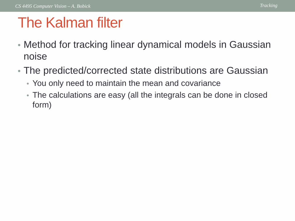
The Kalman filter • Method for tracking linear dynamical models in Gaussian
noise • The predicted/corrected state distributions are Gaussian
• You only need to maintain the mean and covariance • The calculations are easy (all the integrals can be done in closed
form)

Tracking CS 4495 Computer Vision – A. Bobick
Propagation of Gaussian densities

Tracking CS 4495 Computer Vision – A. Bobick
The Kalman Filter: 1D state
( )10 ,, −tt yyXP
( )tt yyXP ,,0
Predict Correct
Given corrected state from previous time
step and all the measurements up to
the current one, predict the
distribution over the current step
Given prediction of state and current measurement, update prediction of state
Time advances (from t–1 to t)
−−tt σµ ,
Mean and std. dev. of predicted state:
++tt σµ ,
Mean and std. dev. of corrected state:
Make measurement

Tracking CS 4495 Computer Vision – A. Bobick
1D Kalman filter: Prediction • Linear dynamic model defines predicted state evolution,
with noise •
• Want to estimate distribution for next predicted state
( )21,~ dtt dxNX σ−
( ) ( ) ( ) 1101110 ,,||,,| −−−−− ∫= ttttttt dXyyXPXXPyyXP

Tracking CS 4495 Computer Vision – A. Bobick
1D Kalman filter: Prediction • Linear dynamic model defines predicted state evolution,
with noise • Want to estimate distribution for next predicted state
• Update the mean:
• Update the variance:
+−
− = 1tt dµµ
( ) ( )210 )(,,, −−− = tttt NyyXP σµ
21
22 )()( +−
− += tdt dσσσ
( )21,~ dtt dxNX σ−

Tracking CS 4495 Computer Vision – A. Bobick
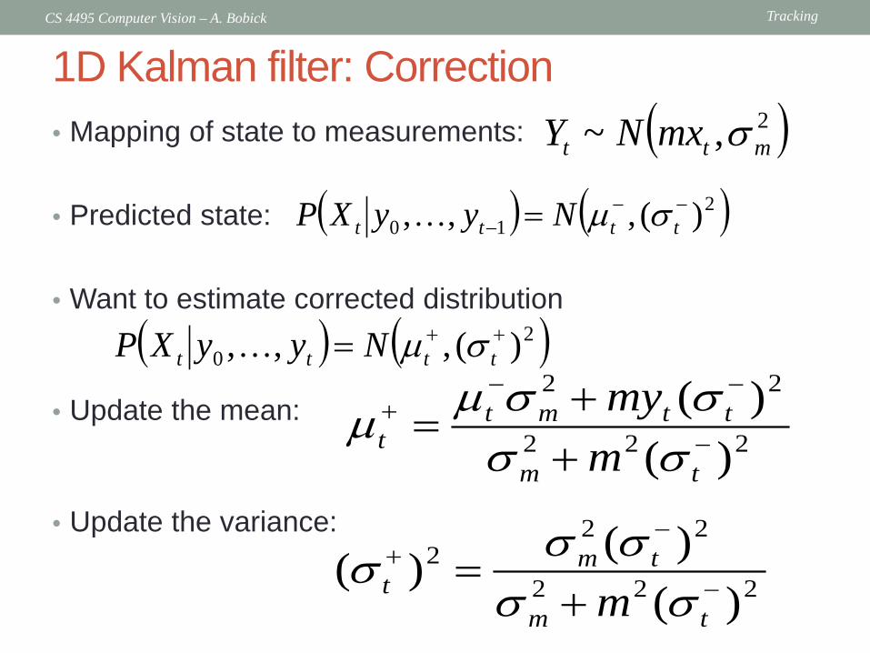
1D Kalman filter: Correction • Mapping of state to measurements:
• Predicted state:
• Want to estimate corrected distribution
( )2,~ mtt mxNY σ
( ) ( )210 )(,,, −−− = tttt NyyXP σµ
( ) ( ) ( )( ) ( )∫ −
−=ttttt
tttttt dXyyXPXyP
yyXPXyPyyXP10
100 ,,||
,,||,,|

Tracking CS 4495 Computer Vision – A. Bobick
1D Kalman filter: Correction • Mapping of state to measurements:
• Predicted state:
• We define the corrected distribution to be:
( )2,~ mtt mxNY σ
( ) ( )210 )(,,, −−− = tttt NyyXP σµ
( ) ( )20 , , , ( )t t t tP X y y N µ σ+ +≡
Tracking CS 4495 Computer Vision – A. Bobick
1D Kalman filter: Correction • Mapping of state to measurements:
• Predicted state:
• Want to estimate corrected distribution
• Update the mean:
• Update the variance:
( )2,~ mtt mxNY σ
( ) ( )210 )(,,, −−− = tttt NyyXP σµ
( ) ( )20 )(,,, ++= tttt NyyXP σµ
222
22
)()(
−
−−+
++
=tm
ttmtt m
myσσσσµµ
222
222
)()()( −
−+
+=
tm
tmt m σσ
σσσ
Tracking CS 4495 Computer Vision – A. Bobick
1D Kalman filter: Correction
From:
• What is this? • The weighted average of prediction and measurement
based on variances!
222
22
)()(
−
−−+
++
=tm
ttmtt m
myσσσσµµ
22
2
22
2
( )
( )
t m tt
tm
t
ym m
m
µ σ σµ
σ σ
−−
+
−
+=
+
Measurement guess of x
Variance of x computed from the measurement
Prediction of x
Variance of prediction

Tracking CS 4495 Computer Vision – A. Bobick
Prediction vs. correction
• What if there is no prediction uncertainty •
• What if there is no measurement uncertainty
−+ = tt µµ 0)( 2 =+tσ
222
22
)()(
−
−−+
++
=tm
ttmtt m
myσσσσµµ 222
222
)()()( −
−+
+=
tm
tmt m σσ
σσσ
?)0( =mσ
?)0( =−tσ
myt
t =+µ 0)( 2 =+tσ
The measurement is ignored!
The prediction is ignored!
Tracking CS 4495 Computer Vision – A. Bobick
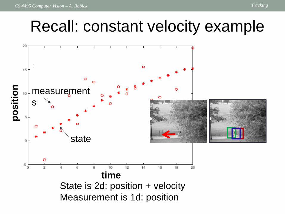
Recall: constant velocity example
State is 2d: position + velocity Measurement is 1d: position
measurements
state
time
posi
tion

Tracking CS 4495 Computer Vision – A. Bobick
Kalman filter processing
time
o state
x measurement
* predicted mean estimate
+ corrected mean estimate
bars: variance estimates before and after measurements
Constant velocity model po
sitio
n

Tracking CS 4495 Computer Vision – A. Bobick
Kalman filter processing
time
o state
x measurement
* predicted mean estimate
+ corrected mean estimate
bars: variance estimates before and after measurements
Constant velocity model po
sitio
n

Tracking CS 4495 Computer Vision – A. Bobick
Kalman filter processing
time
o state
x measurement
* predicted mean estimate
+ corrected mean estimate
bars: variance estimates before and after measurements
Constant velocity model po
sitio
n

Tracking CS 4495 Computer Vision – A. Bobick
Kalman filter processing
time
o state
x measurement
* predicted mean estimate
+ corrected mean estimate
bars: variance estimates before and after measurements
Constant velocity model po
sitio
n

Tracking CS 4495 Computer Vision – A. Bobick
Kalman filter: General case (> 1dim)
PREDICT CORRECT
+−
− = 1ttt xDx
tdTtttt DD Σ+Σ=Σ +
−−
1( )−−+ −+= tttttt xMyKxx
( ) −+ Σ−=Σ tttt MKI
( ) 1−−− Σ+ΣΣ=tm
Tttt
Tttt MMMK
What if state vectors have more than one dimension?
More weight on residual when measurement error covariance approaches 0.

Tracking CS 4495 Computer Vision – A. Bobick
Kalman filter pros and cons • Pros
• Simple updates, compact and efficient
• Cons • Unimodal distribution, only single hypothesis • Restricted class of motions defined by linear model
• Extensions call “Extended Kalman Filtering”
• So what might we do if not Gaussian? Or even unimodal?

Tracking CS 4495 Computer Vision – A. Bobick
Find out next time! (Actually next Thurs)