CS 376 Introduction to Computer Graphics 02 / 07 / 2007 Instructor: Michael Eckmann.

CS 376Introduction to Computer Graphics

02 / 07 / 2007

Instructor: Michael Eckmann

Michael Eckmann - Skidmore College - CS 376 - Spring 2007

Today’s Topics• Questions?• Polygons• Determining if a point is in the interior of a polygon• Polygon filling algorithm• tiling• halftoning• dithering• antialiasing polygons


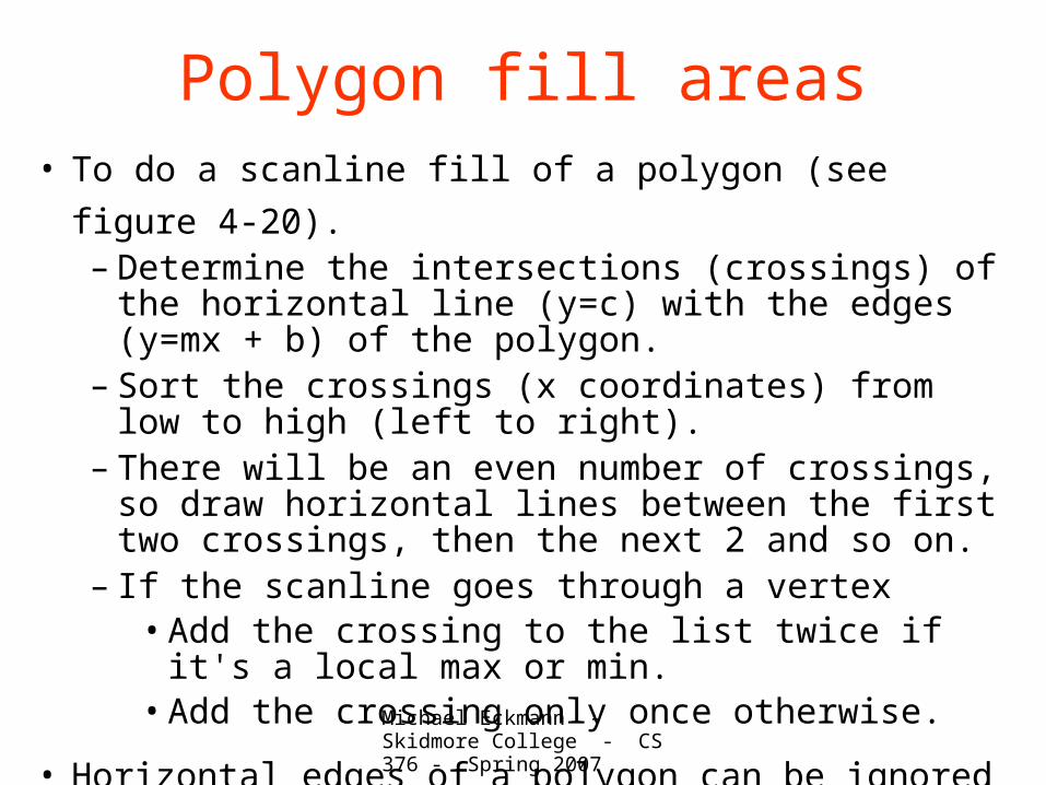
Polygon fill areas• To do a scanline fill of a polygon (see figure 4-20).

– Determine the intersections (crossings) of the horizontal line (y=c) with the edges (y=mx + b) of the polygon.

– Sort the crossings (x coordinates) from low to high (left to right).

– There will be an even number of crossings, so draw horizontal lines between the first two crossings, then the next 2 and so on.

– If the scanline goes through a vertex• Add the crossing to the list twice if it's a local max or min.• Add the crossing only once otherwise.

• Horizontal edges of a polygon can be ignored (not turned on.)

• Example on board.


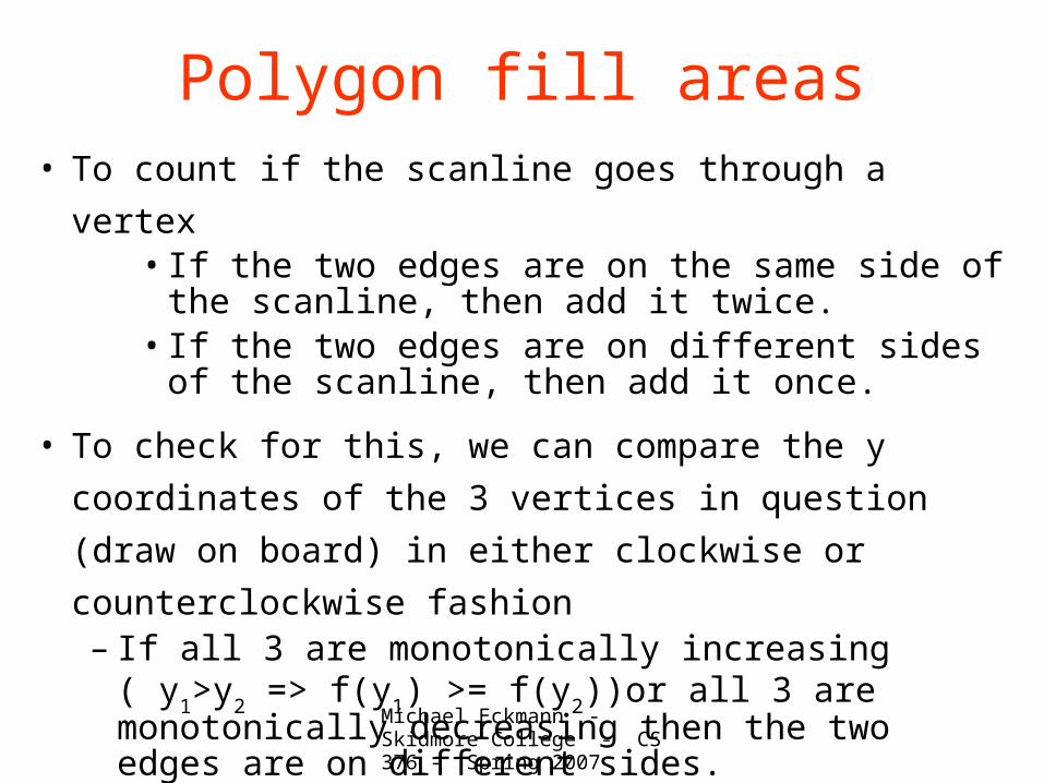
Polygon fill areas• To count if the scanline goes through a vertex

• If the two edges are on the same side of the scanline, then add it twice.

• If the two edges are on different sides of the scanline, then add it once.

• To check for this, we can compare the y coordinates of the 3

vertices in question (draw on board) in either clockwise or

counterclockwise fashion– If all 3 are monotonically increasing ( y

1>y

2 => f(y

1) >= f(y

2))or

all 3 are monotonically decreasing then the two edges are on different sides.


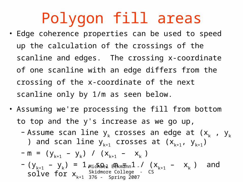
Polygon fill areas• Edge coherence properties can be used to speed up the calculation of the

crossings of the scanline and edges. The crossing x-coordinate of one

scanline with an edge differs from the crossing of the x-coordinate of the

next scanline only by 1/m as seen below.

• Assuming we're processing the fill from bottom to top and the y's

increase as we go up, – Assume scan line y

k crosses an edge at (x

k , y

k ) and scan line y

k+1

crosses at (xk+1

, yk+1

)

– m = (yk+1

– yk) / (x

k+1 – x

k )

– (yk+1

– yk) = 1, so, m = 1 / (x

k+1 – x

k ) and solve for x

k+1

– So, scan line yk+1

crosses that edge at (xk + 1/m, y

k )


Polygon fill areas• Efficient polygon filling

– 1) proceed around edges in a clockwise or counterclockwise fashion– 2) store each edge in an edge table– 3) sort the edges based on the minimum y in the edge– 4) process the scanlines in a bottom to top order– 5) when the current scanline reaches the lower endpoint (with the

min y) of the edge, that edge becomes active– 6) active edges are sorted by their x coordinates (left to right)– During any given scanline non-active edges can be marked as either

finished, or not yet active. Horizontal edges are ignored.

• Example on board.


Polygon fill areas• Masks

– Besides being filled with a solid color, polygons are sometimes filled with patterns. The process of filling an area with a pattern is called tiling.

– Fill patterns can be stored as rectangular arrays. The arrays are called masks and they are applied to the fill area and are usually smaller than the area to be filled.

– The mask needs a starting position within the area to be filled. Starting at this position the mask is replicated both vertically and horizontally.

– If the mask is an m n array, and starting position is (0,0) a pixel at (x, y) will be drawn with the color in mask((x mod n), (y mod m)).

– Example on board.


Polygon fill areas• Section 10.9 Halftoning and dithering

– When there are very few intensity levels available (e.g. 2, black & white) to be displayed, halftoning is a technique that can provide more intensities by trading off addressability.

– Newspapers show grey level photos by displaying black circles. The black circles vary in size according to how dark that part of the photo should be.

– In graphics systems this halftoning technique is approximated with halftone patterns. Halftone patterns are typically n n squares of pixels where the number of pixels turned on in that pattern correspond to the intensity desired.


Polygon fill areas• How is halftoning a tradeoff between intensities and addressability

(resolution) ?


Polygon fill areas• Guidelines to creating halftoning patterns

– With halftoning, one thing to be careful about is that the patterns can become apparent. That is undesirable. The intent is to have the viewer see the increase in intensities without noticing unintentional patterns.

– Avoid only horizontal or vertical or diagonal pixels on in the patterns to reduce the possibility of “streaks”.

– Further it is good to approximate the way that newspapers do it --- that is, concentrate on turning on pixels in the center of the pattern at each successive intensity.

– To minimize unintentional patterns to be displayed, we can evolve each successive grid pattern by copying it and turning on an additional pixel.

• See next slide figure 10-40.


Polygon fill areas


Polygon fill areas• Dithering

– Dithering refers to techniques for approximating halftones but without reducing addressability (resolution).

– An nn dither matrix Dn is used to detemine if a pixel should

be on or off. – The matrix is filled with the numbers from 0 to n2 – 1– on page 589 (equation 10-49) there's a mistake, it should be the

dither matrix D4

15 7 13 5 3 11 1 912 4 14 6 0 8 2 10


Polygon fill areas• Example of dither matrix D

4

15 7 13 5 3 11 1 912 4 14 6 0 8 2 10

– For some pixel (x, y) an intensity level I(x,y) between 0 and n2 is desired. Compute i = x mod n and j = y mod n to find which element (i,j) of the matrix D

n to compare to the desired intensity.

– If I(x,y) > Dn(i,j) then the pixel is turned on, otherwise it is not.

– This has the effect of different intensities, without reducing resolution. But what gets lost?


Antialiasing Polygons• Edges of polygons are lines. Lines (and therefore edges) have aliasing

problems when made discrete. Antialiasing edges of polygons can be

done using similar techniques as were used with lines. One way

described below is the way I described antialiasing Bresenham lines.

• During scanline fill of a polygon, if the edge falls between two pixels on

the scanline, then the intensities of the pixels depend on how close to the

centers of the two pixels the line falls.

• The pixel at (xj, y

k): could be set to have x

j+1 – x and x

j+1

• The pixel at (xj+1

, yk) would then be set to have x – x

j

• Pixels that fall fully within the interior of a polygon are set to full

intensity.


Geometric Transformations (2D)• Reading: 5.1- 5.9 (2D geometric transformations)

• Translations

• Rotations

• Scaling

• Homogeneous Coordinates

• Shearing

• Reflections


Matrices• An m by n matrix is a two dimensional array of values with m rows and n

columns. Points are typically represented by column matrices (meaning they

have multiple rows, but only 1 column)

• Matrix multiplication (3x3 times a 3x3 yields a 3x3 matrix)( a b c ) ( j k l ) ( aj+bm+cp ak+bn+cq al+bo+cr ) ( d e f ) ( m n o ) = ( dj+em+fp dk+en+fq dl+eo+fr ) ( g h i ) ( p q r ) ( gj+hm+ip gk+hn+iq gl+ho+ir )

• Matrix multiplication (2x2 times a 2x1 yields a 2x1 column matrix)( a b ) ( x ) = ( ax+by )( c d ) ( y ) ( cx+dy )

• A 2x2 matrix times a 2x1 matrix (a point) yields another point.

• Matrix multiplication is associative. ABC = (AB)C = A(BC).


Translations (2D)• Recall the idea that for the circle algorithm that we did computations

assuming the circle's center was the origin. Then when we plotted the

points we offset the calculated point by the actual center by just adding

the respective coordinates. What we did there was perform a translation.

• Translation is a transformation on an object that simply moves it to a

different position somewhere else within the same coordinate system.

To translate an object we translate each of its vertices (points).

• To translate a 2d point (x1, y

1) by t

x in the x direction and t

y in the y

direction, we simply calculate the new coordinates to be:

• (x2, y

2) = (x

1 + t

x , y

1 + t

y )


Scaling (2D)• Scaling is a transformation on an object that changes its size. Just as the

translation could have been different amounts in x and y, you can scale x

and y by different factors.

• Scaling is a transformation on an object that changes its size within the

same coordinate system. To scale an object we scale each of its vertices

(points).

• To scale a 2d point (x1, y

1) by s

x in the x direction and s

y in the y

direction, we simply calculate the new coordinates to be:

• (x2, y

2) = (s

xx

1 , s

yy

1 )

• Example on the board of scaling a line segment from say 2,3 to 2,7


Rotation (2D)• Rotation is a transformation on an object that changes its position in a

specific way (by rotating the object some angle about an axis).

• Rotations in the x-y plane are about an axis parallel to z. The point of

intersection of the rotation axis with the x-y plane is the pivot point.

• We need to specify the angle and pivot point about which the object is to

be rotated.

• To rotate an object we rotate each of its vertices (points).

• Positive angles are in the counterclockwise direction.


Rotation (2D)• To rotate a 2d point (x

1, y

1) an arbitrary angle of B, about the origin as a

pivot point do the following.

• From the diagram on the board (also see figure 5-4 in the text) we have:

sin(A + B) = y2 / r => y

2 = r sin(A + B)

cos(A + B) = x2 / r x

2 = r cos(A + B)

sin(A) = y1 / r y

1 = r sin(A)

cos(A) = x1 / r x

1 = r cos(A)

• Known equalities exist for sin(A+B) and cos(A+B)sin(A + B) = sin(A) cos(B) + cos(A) sin(B)cos(A + B) = cos(A) cos(B) – sin(A) sin(B)


Rotation (2D)• Solve for x

2 and y

2.

• x2 = r cos(A + B) = r cos(A) cos(B) – r sin(A) sin(B)

= x1 cos(B) – y

1 sin(B)

• y2 = r sin(A + B) = r sin(A) cos(B) + r cos(A) sin(B)

= y1 cos(B) + x

1 sin(B)

• So, (x2, y

2) = (x

1 cos(B) – y

1 sin(B) , y

1 cos(B) + x

1 sin(B)

)

• This will rotate a point (x1, y

1) an angle of B about the pivot point of the

origin.


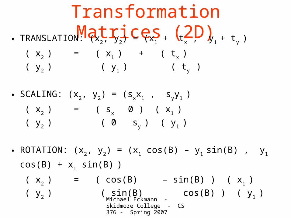
Transformation Matrices (2D)• TRANSLATION: (x

2, y

2) = (x

1 + t

x , y

1 + t

y )

( x2 ) = ( x

1 ) + ( t

x )

( y2 ) ( y

1 ) ( t

y )

• SCALING: (x2, y

2) = (s

xx

1 , s

yy

1 )

( x2 ) = ( s

x 0 ) ( x

1 )

( y2 ) ( 0 s

y ) ( y

1 )

• ROTATION: (x2, y

2) = (x

1 cos(B) – y

1 sin(B) , y

1 cos(B) + x

1 sin(B)

)

( x2 ) = ( cos(B)

– sin(B) ) ( x

1 )

( y2 ) ( sin(B)

cos(B) ) ( y

1 )


Homogeneous Coordinates• Translations, Scales and Rotations can be done as described in the previous

slides.

• What was not described was rotation about an arbitrary pivot point. In

addition to the matrix multiplication involved, a vector (column matrix) add

would need to be added in.

• So, both translations and rotations have an add of a column matrix. In

addition, rotations and scales have matrix multiplications as well.

• To be able to represent all transformations only with matrix multiplications

(without additions of column matrices), we use homogeneous coordinates.


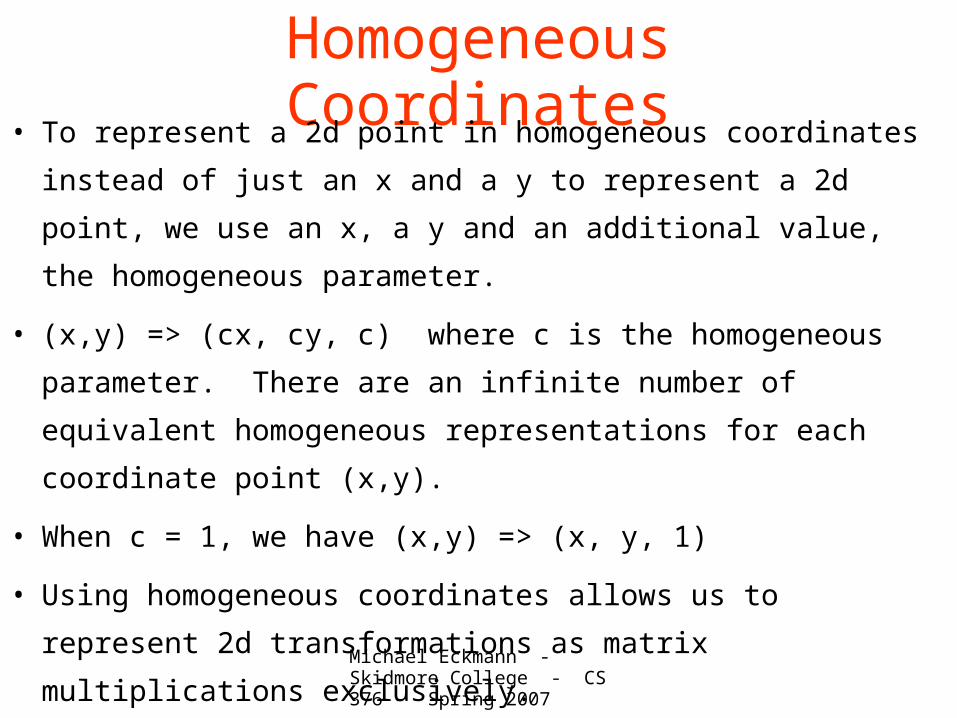
Homogeneous Coordinates• To represent a 2d point in homogeneous coordinates instead of just an x and

a y to represent a 2d point, we use an x, a y and an additional value, the

homogeneous parameter.

• (x,y) => (cx, cy, c) where c is the homogeneous parameter. There are an

infinite number of equivalent homogeneous representations for each

coordinate point (x,y).

• When c = 1, we have (x,y) => (x, y, 1)

• Using homogeneous coordinates allows us to represent 2d transformations as

matrix multiplications exclusively.


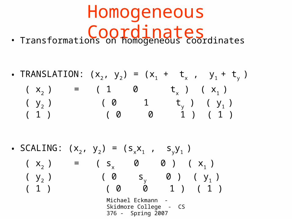
Homogeneous Coordinates• Transformations on homogeneous coordinates

• TRANSLATION: (x2, y

2) = (x

1 + t

x , y

1 + t

y )

( x2 ) = ( 1 0 t

x ) ( x

1 )

( y2 ) ( 0 1 t

y ) ( y

1 )

( 1 ) ( 0 0 1 ) ( 1 )

• SCALING: (x2, y

2) = (s

xx

1 , s

yy

1 )

( x2 ) = ( s

x 0 0 ) ( x

1 )

( y2 ) ( 0 s

y 0 ) ( y

1 )

( 1 ) ( 0 0 1 ) ( 1 )


Homogeneous Coordinates• Transformations on homogeneous coordinates

• ROTATION: (x2, y

2) = (x

1 cos(B) – y

1 sin(B) , y

1 cos(B) + x

1 sin(B)

)

( x2 ) = (cos(B)

– sin(B) 0 ) ( x

1 )

( y2 ) (sin(B)

cos(B) 0 ) ( y

1 )

( 1 ) ( 0 0 1 ) ( 1 )

• These three transform matrices are sometimes written as– T(t

x,t

y)

– S(sx,s

y)

– R(B)


Scaling a line segment• Let's look at this example on the board. Example: Scale a line segment from (3,2)

to (5,2) by 2 in the x-direction.

( x0 ) ( 2

0 0 ) ( 3

) ( 6 )

( y0 ) = ( 0 1

0 ) ( 2

) = ( 2 )

( 1 ) ( 0 0 1 ) ( 1 ) ( 1 )

• And the other endpoint:

( xend

) ( 2 0 0 ) ( 5

) ( 10 )

( yend

) = ( 0 1 0 ) ( 2

) = ( 2 )

( 1 ) ( 0 0 1 ) ( 1 ) ( 1 )

• Problem: The line segment (3,2) to (5,2) when scaled by 2 in x-direction gives a

line segment from (6,2) to (10, 2). Yes it's original length in the x-direction was

2 and now it is 4, but the line also was translated. Let's see it on the board.


Fixed point scaling• Specify a point that will remain fixed after the scaling. This is the fixed-point.

• Let's scale the same line segment but this time fix the left endpoint (3,2).

• To do this, we need to:– a) first translate (3, 2) to the origin– b) scale by 2 in x-direction (like before)– c) then translate the origin back to (3, 2)

• This will yield a matrix multiplication McM

bM

a = M

fps which we will then

multiply Mfps

P, where P is a homogeneous point, to get the transformed point.

• Notice the order: matrix Ma is closest to the point, then M

b then M

c


Fixed point scaling• a) the matrix to translate (3, 2) to the origin is this:

(1 0 -3)(0 1 -2)(0 0 1)

• b) the matrix to scale by 2 in x direction is this:(2 0 0)(0 1 0)(0 0 1)

• c) the matrix to translate the origin back to (3, 2) is this:(1 0 3)(0 1 2)(0 0 1)


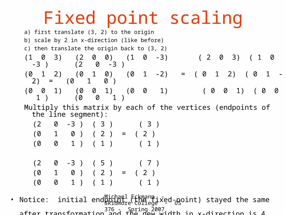
Fixed point scalinga) first translate (3, 2) to the origin

b) scale by 2 in x-direction (like before)

c) then translate the origin back to (3, 2)

(1 0 3) (2 0 0) (1 0 -3) ( 2 0 3) ( 1 0 -3 ) (2 0 -3 )(0 1 2) (0 1 0) (0 1 -2) = ( 0 1 2) ( 0 1 -2) = (0 1 0 )(0 0 1) (0 0 1) (0 0 1) ( 0 0 1) ( 0 0 1 ) (0 0 1 )Multiply this matrix by each of the vertices (endpoints of the line segment): (2 0 -3 ) ( 3 ) ( 3 ) (0 1 0 ) ( 2 ) = ( 2 ) (0 0 1 ) ( 1 ) ( 1 )

(2 0 -3 ) ( 5 ) ( 7 ) (0 1 0 ) ( 2 ) = ( 2 ) (0 0 1 ) ( 1 ) ( 1 )

• Notice: initial endpoint (the fixed-point) stayed the same after transformation and the new

width in x-direction is 4 (which is 2 the scale factor * 2 the original length).


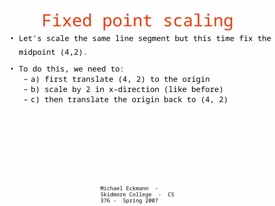
Fixed point scaling• Let's scale the same line segment but this time fix the midpoint (4,2).

• To do this, we need to:– a) first translate (4, 2) to the origin– b) scale by 2 in x-direction (like before)– c) then translate the origin back to (4, 2)


Fixed point scalinga) first translate (4, 2) to the origin

b) scale by 2 in x-direction (like before)

c) then translate the origin back to (4, 2)

(1 0 4) (2 0 0) (1 0 -4) ( 2 0 4) ( 1 0 -4 ) (2 0 -4 )(0 1 2) (0 1 0) (0 1 -2) = ( 0 1 2) ( 0 1 -2) = (0 1 0 )(0 0 1) (0 0 1) (0 0 1) ( 0 0 1) ( 0 0 1 ) (0 0 1 )Multiply this matrix by each of the vertices (endpoints of the line segment): (2 0 -4 ) ( 3 ) ( 2 ) (0 1 0 ) ( 2 ) = ( 2 ) (0 0 1 ) ( 1 ) ( 1 )

(2 0 -4 ) ( 5 ) ( 6 ) (0 1 0 ) ( 2 ) = ( 2 ) (0 0 1 ) ( 1 ) ( 1 )

• Notice: the line segment stretched equally left and right from the middle. The new width

in x-direction is 4 (which is 2 the scale factor * 2 the original length).

CS 376 Introduction to Computer Graphics 02 / 07 / 2007 Instructor: Michael Eckmann.

Documents

Transcript of CS 376 Introduction to Computer Graphics 02 / 07 / 2007 Instructor: Michael Eckmann.