CS 361A 1

CS 361A CS 361A (Advanced Data Structures and Algorithms)(Advanced Data Structures and Algorithms)

Lecture 19 (Dec 5, 2005)

Nearest Neighbors: Dimensionality Reduction and

Locality-Sensitive Hashing

Rajeev Motwani

CS 361A 2

Metric SpaceMetric Space• Metric Space (M,D)

– For points p,q in M, D(p,q) is distance from p to q

– only reasonable model for high-dimensional geometric space

• Defining Properties– Reflexive: D(p,q) = 0 if and only if p=q

– Symmetric: D(p,q) = D(q,p)

– Triangle Inequality: D(p,q) is at most D(p,r)+D(r,q)

• Interesting Cases– M points in d-dimensional space

– D Hamming or Euclidean Lp-norms

CS 361A 3

High-Dimensional Near NeighborsHigh-Dimensional Near Neighbors • Nearest Neighbors Data Structure

– Given – N points P={p1, …, pN} in metric space (M,D)

– Queries – “Which point pP is closest to point q?”

– Complexity – Tradeoff preprocessing space with query time

• Applications – vector quantization

– multimedia databases

– data mining

– machine learning

– …

CS 361A 4

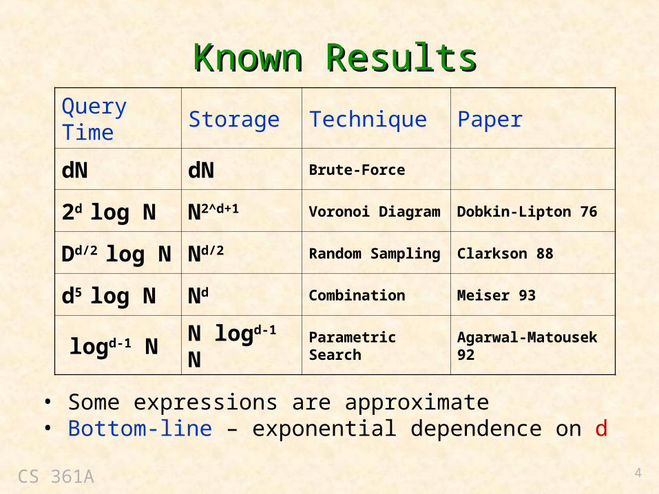
Known ResultsKnown ResultsQuery Time

Storage Technique Paper

dN dN Brute-Force

2d log N N2^d+1 Voronoi Diagram Dobkin-Lipton 76

Dd/2 log N Nd/2 Random Sampling Clarkson 88

d5 log N Nd Combination Meiser 93

logd-1 N N logd-1 N Parametric Search Agarwal-Matousek 92

• Some expressions are approximate• Bottom-line – exponential dependence on d

CS 361A 5

Approximate Nearest NeighborApproximate Nearest Neighbor• Exact Algorithms

– Benchmark – brute-force needs space O(N), query time O(N)

– Known Results – exponential dependence on dimension

– Theory/Practice – no better than brute-force search

• Approximate Near-Neighbors

– Given – N points P={p1, …, pN} in metric space (M,D)

– Given – error parameter >0

– Goal – for query q and nearest-neighbor p, return r such that

• Justification– Mapping objects to metric space is heuristic anyway

– Get tremendous performance improvement

p)ε)D(q,(1r)D(q,

CS 361A 6

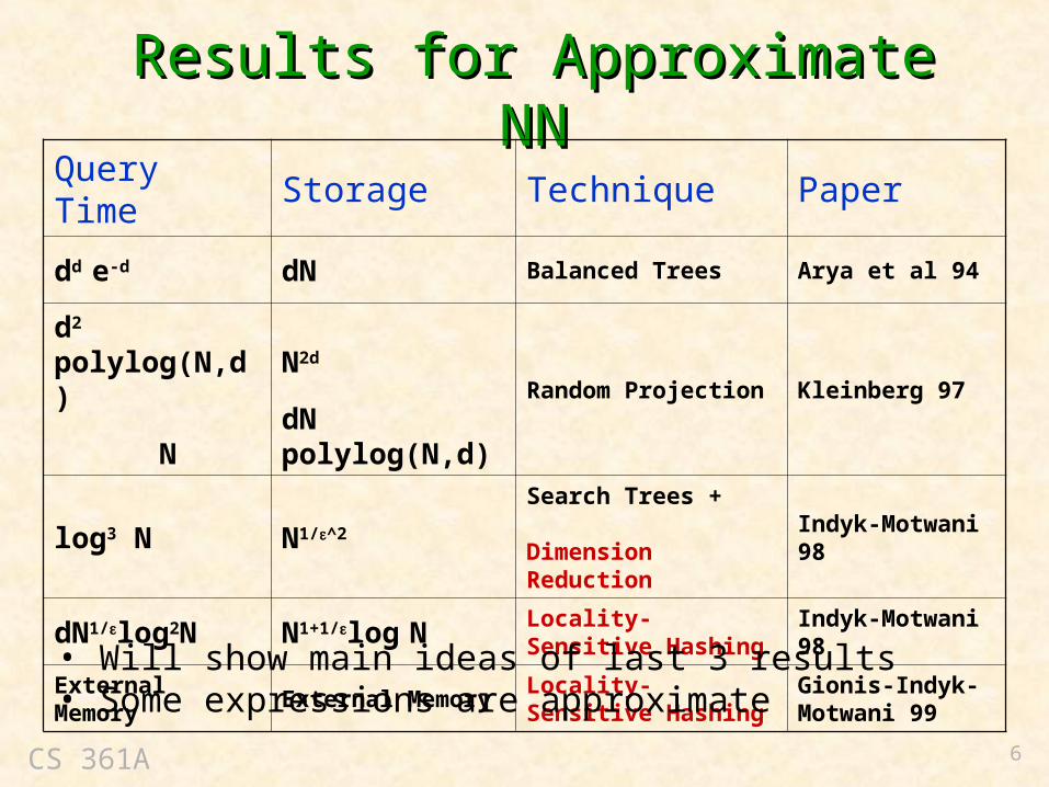
Results for Approximate NNResults for Approximate NN

Query Time Storage Technique Paper

dd e-d dN Balanced Trees Arya et al 94

d2 polylog(N,d)

N

N2d

dN polylog(N,d)Random Projection Kleinberg 97

log3 N N1/^2Search Trees + Dimension Reduction

Indyk-Motwani 98

dN1/log2N N1+1/log NLocality-Sensitive Hashing

Indyk-Motwani 98

External Memory External MemoryLocality-Sensitive Hashing

Gionis-Indyk-Motwani 99

• Will show main ideas of last 3 results • Some expressions are approximate

CS 361A 7

Approximate r-Near NeighborsApproximate r-Near Neighbors• Given – N points P={p1,…,pN} in metric space (M,D)

• Given – error parameter >0, distance threshold r>0

• Query – If no point p with D(q,p)<r, return FAILURE

– Else, return any p’ with D(q,p’)< (1+)r

• Application – Solving Approximate Nearest Neighbor

– Assume maximum distance is R

– Run in parallel for

– Time/space – O(log R) overhead

– [Indyk-Motwani] – reduce to O(polylog n) overhead

R,,ε)(1,ε)(1 ε),(1 1, r 32

CS 361A 8

Hamming MetricHamming Metric• Hamming Space

– Points in M: bit-vectors {0,1}d (can generalize to {0,1,2,…,q}d)

– Hamming Distance: D(p,q) = # of positions where p,q differ

• Remarks– Simplest high-dimensional setting

– Still useful in practice

– In theory, as hard (or easy) as Euclidean space

– Trivial in low dimensions

• Example– Hypercube in d=3 dimensions

– {000, 001, 010, 011, 100, 101, 110, 111}

CS 361A 9

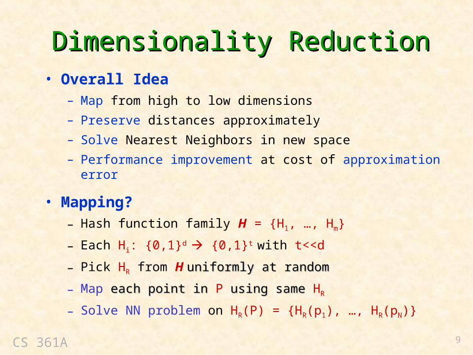
Dimensionality ReductionDimensionality Reduction• Overall Idea

– Map from high to low dimensions

– Preserve distances approximately

– Solve Nearest Neighbors in new space

– Performance improvement at cost of approximation error

• Mapping?– Hash function family H = {H1, …, Hm}

– Each Hi: {0,1}d {0,1}t with t<<d

– Pick HR from H uniformly at randomuniformly at random

– Map each point in each point in P using same using same HR

– Solve NN problem on HR(P) = {HR(p1), …, HR(pN)}

CS 361A 10

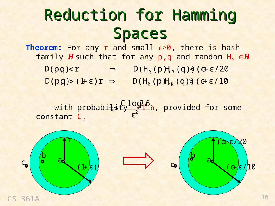
Reduction for Hamming SpacesReduction for Hamming SpacesTheorem: For any r and small >0, there is hash family H such that

for any p,q and random HR H

with probability >1-, provided for some constant C,

ε/10)t(c(q))H(p),D(Hε)r(1q)D(p,

ε/20)t(c(q))H(p),D(Hrq)D(p,

RR

RR

2ε

2/δ log Ct

c ab

ε)r(1

r

ca

b

ε/10)t(c

ε/20)t(c

CS 361A 11

RemarksRemarks• For fixed threshold r, can distinguish between

– Near D(p,q) < r

– Far D(p,q) > (1+ε)r

• For N points, need

• Yet, can reduce to O(log N)-dimensional space, while approximately preserving distances

• Works even if points not known in advance

2Nδ

CS 361A 12

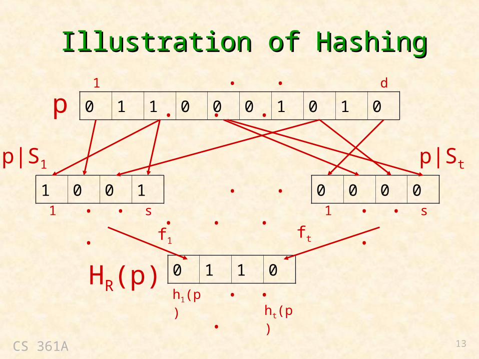
Hash FamilyHash Family• Projection Function

– Let S be ordered, multiset of s indexes from {1,…,d}

– p|S:{0,1}d {0,1}s projects p into s-dimensional subspace

– Example• d=5, p=01100• s=3, S={2,2,4} p|S = 110

• Choosing hash function HR in H– Repeat for i=1,…,t

• Pick Si randomly (with replacement) from {1…d}• Pick random hash function fi:{0,1}s {0,1}• hi(p)=fi(p|Si)

– HR(p) = (h1(p), h2(p),…,ht(p))

• Remark – note similarity to Bloom Filters

CS 361A 13

Illustration of HashingIllustration of Hashing

0 1 1 0 0 0 1 0 1 0

1 0 0 1 0 0 0 0

1 d . . . . .

1 . . . s 1 . . . s

. . . . .

p

p|S1 p|St

0 1 1 0

f1ft

h1(p) . . . ht(p)HR(p)

CS 361A 14

Analysis IAnalysis I

• Choose random index-set S

• Claim: For any p,q

• Why?– p,q differ in D(p,q) bit positions

– Need all s indexes of S to avoid these positions

– Sampling with replacement from {1, …,d}

s

d

q)D(p,1S]qSpPr[

CS 361A 15

Analysis IIAnalysis II

• Choose s=d/r

• Since 1-x<e-x for |x|<1, we obtain

• Thus

q)/rD(p,es

d

q)D(p,1S]qSpPr[

ε/3eS]qSpPr[ε)r(1q)D(p,

eS]qSpPr[rq)D(p,

1

1

CS 361A 16

Analysis IIIAnalysis III

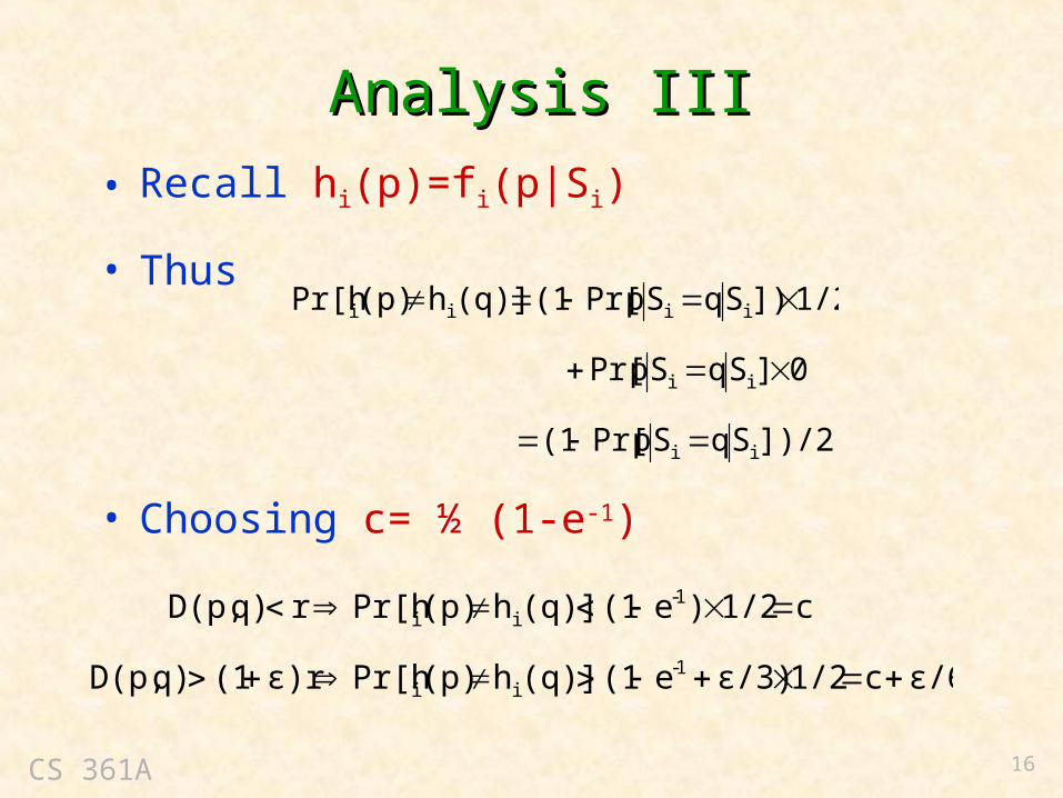
• Recall hi(p)=fi(p|Si)

• Thus

• Choosing c= ½ (1-e-1)

])/2SqSpPr[(1

0]SqSpPr[

1/2])SqSpPr[(1(q)]h(p)Pr[h

ii

ii

iiii

ε/6c1/2ε/3)e(1(q)]h(p)Pr[hε)r(1q)D(p,

c1/2)e(1(q)]h(p)Pr[hrq)D(p,

1-ii

1-ii

CS 361A 17

Analysis IVAnalysis IV• Recall HR(p)=(h1(p),h2(p),…,ht(p))

• D(HR(p),HR(q)) = number of i’s where hi(p), hi(q) differ

• By linearity of expectations

• Theorem almost proved

• For high probability bound, need Chernoff Bound

(q)]h (p)Pr[ht

(q)]h (p)Pr[h (q))]H(p),E[D(H

ii

i iiRR

ε/6)tc((q))]H(p),E[D(Hε)r(1q)D(p,

ct(q))]H(p),E[D(Hrq)D(p,

RR

RR

CS 361A 18

Chernoff BoundChernoff Bound

• Consider Bernoulli random variables X1,X2, …, Xn – Values are 0-1

– Pr[Xi=1] = x and Pr[Xi=0] = 1-x

• Define X = X1+X2+…+Xn with E[X]=nx

• Theorem: For independent X1,…, Xn, for any 0<<1,

nx/3β2eβnxnx-XPr2

2nxP

X nx

CS 361A 19

Analysis VAnalysis V• Define

– Xi=0 if hi(p)=hi(q), and 1 otherwise

– n=t

– Then X = X1+X2+…+Xt = D(HR(p),HR(q))

• Case 1 [D(p,q)<r x=c]

• Case 2 [D(p,q)>(1+ε)r x=c+ε/6]

• Observe – sloppy bounding of constants in Case 2

tc/3/20)( 2

2eεtc/20]txXPr[ε/20)t](cPr[X

tc/3/20)( 2

2eεtc/20]txXPr[ε/10)t](cPr[X

CS 361A 20

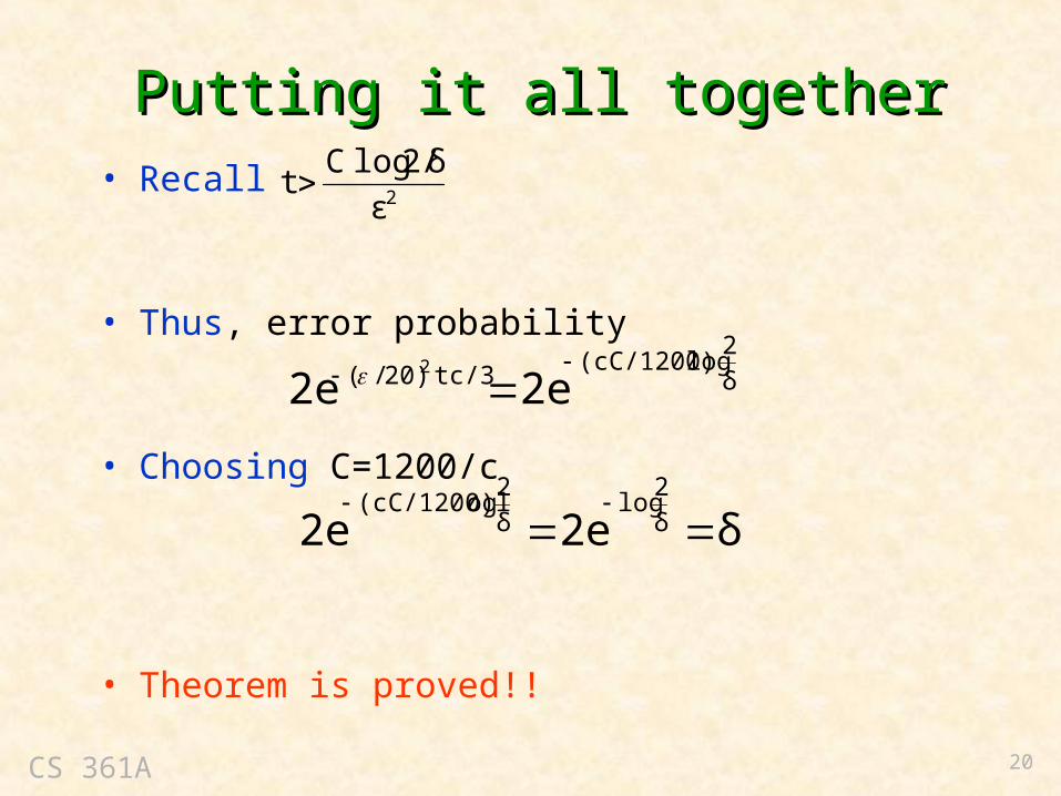
Putting it all togetherPutting it all together• Recall

• Thus, error probability

• Choosing C=1200/c

• Theorem is proved!!

2ε

2/δ log Ct

δ

2log (cC/1200)

tc/320)/( 2e2e2

δ2e2e δ

2log

δ

2og(cC/1200)l

CS 361A 21

Algorithm IAlgorithm I• Set error probability

• Select hash HR and map points p HR(p)

• Processing query q– Compute HR(q)

– Find nearest neighbor HR(p) for HR(q)

– If then return p, else FAILURE

• Remarks– Brute-force for finding HR(p) implies query time

– Need another approach for lower dimensions

N) logO(εt1/poly(N)δ 2

ε)r(1q)D(p,

N) log NO(ε -2

CS 361A 22

Algorithm IIAlgorithm II• Fact – Exact nearest neighbors in {0,1}t requires

– Space O(2t)

– Query time O(t)

• How?– Precompute/store answers to all queries

– Number of possible queries is 2t

• Since

• Theorem – In Hamming space {0,1}d, can solve approximate nearest neighbor with:– Space

– Query time

)O(1/ε2

NN) log O(ε 2

N) logO(εt 2

CS 361A 23

Different MetricDifferent Metric• Many applications have “sparse” points

– Many dimensions but few 1’s

– Example – pointsdocuments, dimensionswords

– Better to view as “sets”

• Previous approach would require large s

• For sets A,B, define

• Observe– A=B sim(A,B)=1

– A,B disjoint sim(A,B)=0

• Question – Handling D(A,B)=1-sim(A,B) ?

BA

BAB)sim(A,

CS 361A 24

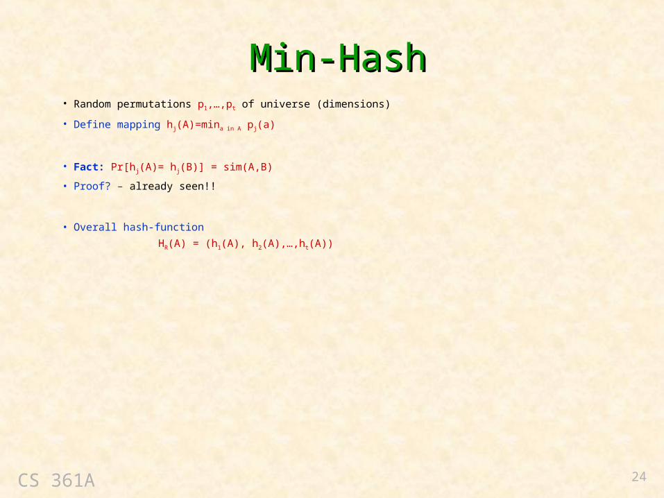
Min-HashMin-Hash• Random permutations p1,…,pt of universe (dimensions)

• Define mapping hj(A)=mina in A pj(a)

• Fact: Pr[hj(A)= hj(B)] = sim(A,B)

• Proof? – already seen!!

• Overall hash-function

HR(A) = (h1(A), h2(A),…,ht(A))

CS 361A 25

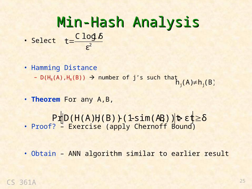
Min-Hash AnalysisMin-Hash Analysis• Select

• Hamming Distance– D(HR(A),HR(B)) number of j’s such that

• Theorem For any A,B,

• Proof? – Exercise (apply Chernoff Bound)

• Obtain – ANN algorithm similar to earlier result

2ε

1/δ log Ct

(B)h(A)h jj

δεtB))tsim(A,-(1 - H(B))D(H(A),Pr

CS 361A 26

GeneralizationGeneralization• Goal

– abstract technique used for Hamming space

– enable application to other metric spaces

– handle Dynamic ANN

• Dynamic Approximate r-Near Neighbors– Fix – threshold r

– Query – if any point within distance r of q, return any point within distance

– Allow insertions/deletions of points in P

• Recall – earlier method required preprocessing all possible queries in hash-range-space…

ε)r(1

CS 361A 27

Locality-Sensitive HashingLocality-Sensitive Hashing• Fix – metric space (M,D), threshold r, error

• Choose – probability parameters Q1 > Q2>0

Definition – Hash family H={h:MS} for (M,D) is called . -sensitive, if for random h and for any p,q in M

• Intuition– p,q are near likely to collide

– p,q are far unlikely to collide

0ε

)Q,Qε,(r, 21

2

1

Qh(p)h(q)Prε)r(1q)D(p,

Qh(p)h(q)Prrq)D(p,

CS 361A 28

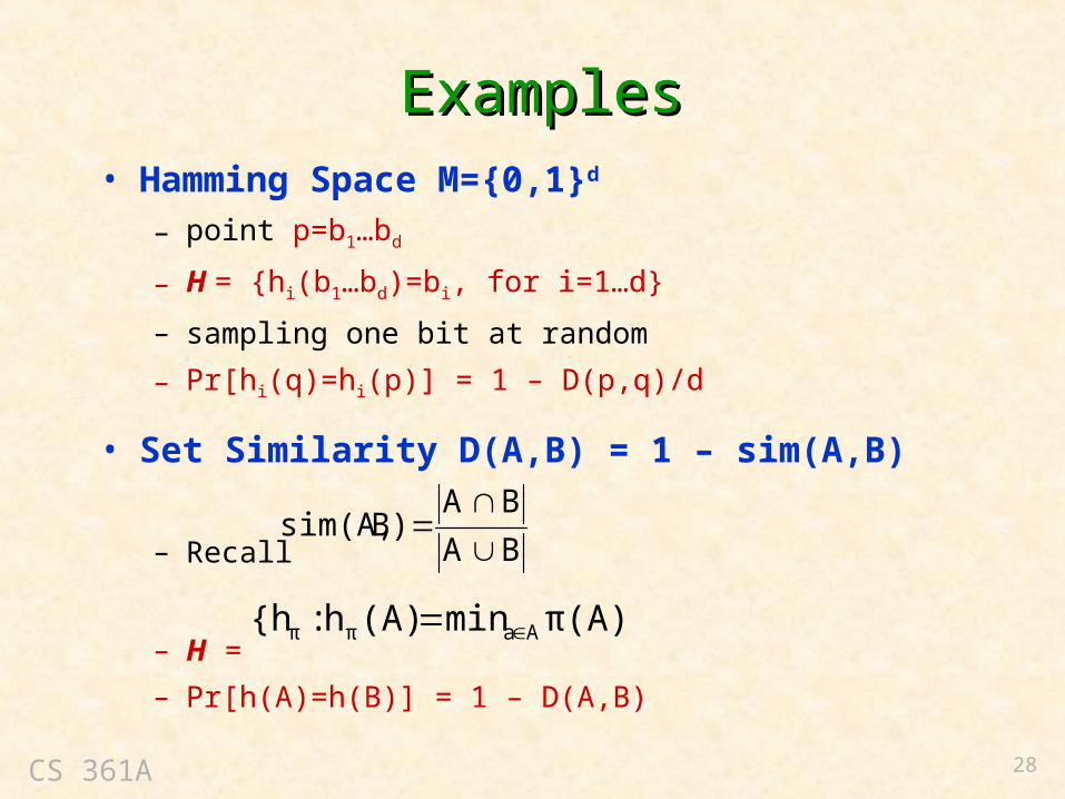
ExamplesExamples• Hamming Space M={0,1}d

– point p=b1…bd

– H = {hi(b1…bd)=bi, for i=1…d}

– sampling one bit at random

– Pr[hi(q)=hi(p)] = 1 – D(p,q)/d

• Set Similarity D(A,B) = 1 – sim(A,B)

– Recall

– H =

– Pr[h(A)=h(B)] = 1 – D(A,B)

BA

BAB)sim(A,

π(A)}min(A)h:{h Aaππ

CS 361A 29

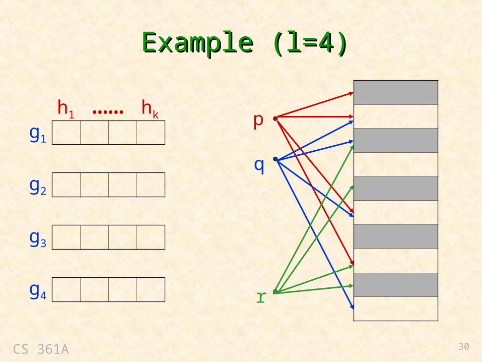
Multi-Index HashingMulti-Index Hashing• Overall Idea

– Fix LSH family H

– Boost Q1, Q2 gap by defining G = H k

– Using G, each point hashes into l buckets

• Intuition– r-near neighbors likely to collide

– few non-near pairs in any bucket

• Define – G = { g | g(p) = h1(p)h2(p)…hk(p) }

– Hamming metric sample k random bits

CS 361A 30

Example (Example (ll=4)=4)

p

q

r

g1

g2

g3

g4

h1 hk……

CS 361A 31

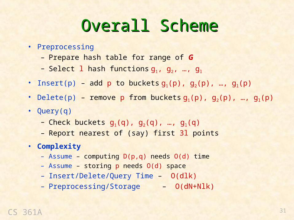
Overall SchemeOverall Scheme• Preprocessing

– Prepare hash table for range of G

– Select l hash functions g1, g2, …, gl

• Insert(p) – add p to buckets g1(p), g2(p), …, gl(p)

• Delete(p) – remove p from buckets g1(p), g2(p), …, gl(p)

• Query(q)

– Check buckets g1(q), g2(q), …, gl(q)

– Report nearest of (say) first 3l points

• Complexity– Assume – computing D(p,q) needs O(d) time

– Assume – storing p needs O(d) space

– Insert/Delete/Query Time – O(dlk)

– Preprocessing/Storage – O(dN+Nlk)

CS 361A 32

Collision Probability vs. DistanceCollision Probability vs. Distance

r r

Q1

Q2

1

0

r rll )Q(11PQP kk,

collcoll

CS 361A 33

Multi-Index versus ErrorMulti-Index versus Error

• Set l=Nz where

Theorem For l=Nz, any query returns r-near neighbor correctly with probability at least 1/6.

• Consequently (ignoring k=O(log N) factors)– Time O(dNz)

– Space O(N1+z)

– Hamming Metric

– Boost Probability – use several parallel hash-tables

2

1

1/Q log

1/Q logz

εl

1z

CS 361A 34

AnalysisAnalysis• Define (for fixed query q)

– p* – any point with D(q,p*) < r

– FAR(q) – all p with D(q,p) > (1+ )r

– BUCKET(q,j) – all p with gj(p) = gj(q)

– Event Esize:

(query cost bounded by O(dl))

– Event ENN: gj(p*) = gj(q) for some j

(nearest point in l buckets is r-near neighbor)

• Analysis

– Show: Pr[Esize] = x > 2/3 and Pr[ENN] = y > 1/2

– Thus: Pr[not(Esize & ENN)] < (1-x) + (1-y) < 5/6

ε

ll

3j)BUCKET(q,FAR(q)1j

CS 361A 35

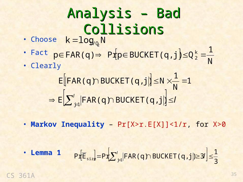
Analysis – Bad CollisionsAnalysis – Bad Collisions• Choose

• Fact

• Clearly

• Markov Inequality – Pr[X>r.E[X]]<1/r, for X>0

• Lemma 1

N

1Qj)BUCKET(q,pPrFAR(q)p k

2

Nlogk21/Q

l

l

1jj)BUCKET(q,FAR(q)E

1N

1Nj)BUCKET(q,FAR(q)E

3

13j)BUCKET(q,FAR(q)Pr EPr

1jsize

ll

CS 361A 36

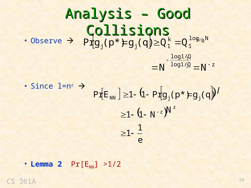
Analysis – Good CollisionsAnalysis – Good Collisions• Observe

• Since l=nz

• Lemma 2 Pr[ENN] >1/2

zlog1/Q

log1/Q

Nlog

1k1jj

NN

QQ(q)g(p*)gPr

2

1

21/Q

e

11

NN11

(q)g(p*)gPr11EPrz

z

jjNN

l

CS 361A 37

Euclidean NormsEuclidean Norms

• Recall

– x=(x1, x2, …, xd) and y=(y1, y2, …, yd) in Rd

– L1-norm

– Lp-norm (for p>1)

d

1i ii1yxyx

p d

1i

piip

yxyx

CS 361A 38

Extension to LExtension to L11-Norm-Norm

• Round coordinates to {1,…M}

• Embed L1-{1,…,M}d into Hamming-{0,1}dM

• Unary Mapping

• Apply algorithm for Hamming Spaces– Error due to rounding of 1/M – Space-Time Overhead due to mapping of d dM

dd11

dd11

yMyyMyd1

xMxxMxd1

00110011)y,,(y

00110011)x,,(x

Ω(1/ε)M

CS 361A 39

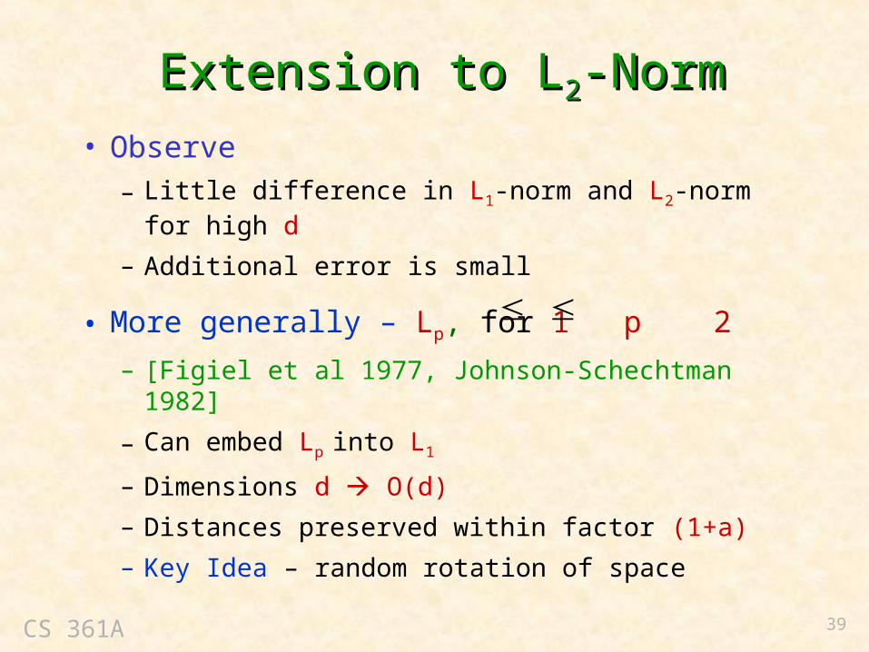
Extension to LExtension to L22-Norm-Norm

• Observe

– Little difference in L1-norm and L2-norm for high d

– Additional error is small

• More generally – Lp, for 1 p 2

– [Figiel et al 1977, Johnson-Schechtman 1982]

– Can embed Lp into L1

– Dimensions d O(d)

– Distances preserved within factor (1+a)

– Key Idea – random rotation of space

CS 361A 40

Improved BoundsImproved Bounds

• [Indyk-Motwani 1998]

– For any Lp-norm

– Query Time – O(log3 N)

– Space –

• Problem – impractical

• Today – only a high-level sketch

)O(1/ε2

N

CS 361A 41

Better ReductionBetter Reduction

• Recall– Reduced Approximate Nearest Neighbors to

Approximate r-Near Neighbors

– Space/Time Overhead – O(log R)

– R = max distance in metric space

• Ring-Cover Trees– Removed dependence on R

– Reduced overhead to O(polylog N)

CS 361A 42

Approximate r-Near NeighborsApproximate r-Near Neighbors

• Idea– Impose regular-grid on Rd

– Decompose into cubes of side length s

– Label cubes with points at distance <r

• Data Structure– Query q – determine cube containing q

– Cube labels – candidate r-near neighbors

• Goals– Small s lower error

– Fewer cubes smaller storage

CS 361A 43

p1

p2

p3

CS 361A 44

Grid AnalysisGrid Analysis• Assume r=1

• Choose

• Cube Diameter =

• Number of cubes =

Theorem – For any Lp-norm, can solve Approx r-Near Neighbor using– Space –

– Time – O(d)

d

εs

εsd 2 dd ) O(ε) /εd(Vol

)O(dNε d

CS 361A 45

Dimensionality ReductionDimensionality Reduction

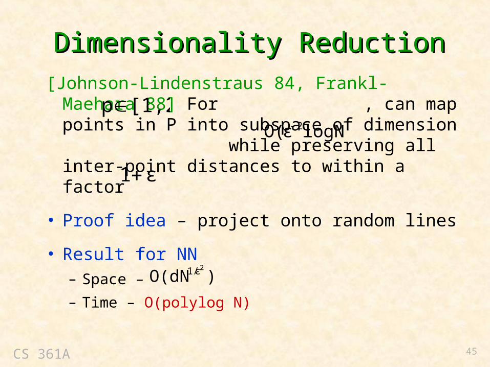
[Johnson-Lindenstraus 84, Frankl-Maehara 88] For , can map points in P into subspace of dimension while preserving all inter-point distances to within a factor

• Proof idea – project onto random lines

• Result for NN– Space –

– Time – O(polylog N)

[1,2]plogN)O(ε 2

ε1

)O(dN21/ε

CS 361A 46

ReferencesReferences• Approximate Nearest Neighbors: Towards

Removing the Curse of Dimensionality P. Indyk and R. Motwani STOC 1998

• Similarity Search in High Dimensions via Hashing A. Gionis, P. Indyk, and R. Motwani VLDB 1999