CRYSTAL09 User's Manual - CRYSTAL Home Page

CRYSTAL092.0.1

User’s ManualFebruary 6, 2013

R. Dovesi1, V.R. Saunders1, C. Roetti1, R. Orlando1,3,C. M. Zicovich-Wilson 1,4, F. Pascale5, B. Civalleri1, K. Doll6,

N.M. Harrison2,7, I.J. Bush8, Ph. D’Arco9, M. Llunell10

1 Theoretical Chemistry Group - University of TurinDipartimento di Chimica IFMVia Giuria 5 - I 10125 Torino - Italy

2 Computational Science & Engineering Department - CCLRC DaresburyDaresbury, Warrington, Cheshire, UK WA4 4AD

3 Universita del Piemonte OrientaleDepartment of Science and Advanced TechnologiesVia Bellini 25/6 - I 15100 Alessandria - Italy

4 Departamento de Fısica, Universidad Autonoma del Estado de Morelos,Av. Universidad 1001, Col. Chamilpa, 62210 Cuernavaca (Morelos) Mexico

5 LCM3B - UMR 7036-CNRSUniversite Henri PoincareNancy BP 239, F54506 Vandœuvre-les-Nancy, Cedex, France

6 Max-Planck-Institut fur FestkorperforschungHeisenbergstrasse 1D-70569 Stuttgart, Germany

7 Department of Chemistry, Imperial CollegeSouth Kensington CampusLondon, U.K.

8 The Numerical Algorithms Group (NAG)Wilkinson House - Jordan Hill RoadOxford OX2 8DR - U.K.

9 Laboratoire de Petrologie, Modelisation des Materiaux et ProcessusUniversite Pierre et Marie Curie,4 Place Jussieu, 75232 Paris CEDEX 05, France

10 Departament de Quımica Fısica, Universitat de BarcelonaDiagonal 647, Barcelona, Spain

1

Contents

Introduction . . . . . . . . . . . . . . . . . . . . . . . . . . . . . . . . . . . . . . . . . 6Typographical Conventions . . . . . . . . . . . . . . . . . . . . . . . . . . . . . 11Acknowledgments . . . . . . . . . . . . . . . . . . . . . . . . . . . . . . . . . . . 12Getting Started - Installation and testing . . . . . . . . . . . . . . . . . . . . . 12

1 Wave function calculation:Basic input route 131.1 Geometry and symmetry information . . . . . . . . . . . . . . . . . . . . . . . . 13

Geometry input for crystalline compounds . . . . . . . . . . . . . . . . . . . . . 14Geometry input for molecules, polymers and slabs . . . . . . . . . . . . . . . . 14Geometry input for polymers with roto translational symmetry . . . . . . . . . 15Geometry input from external geometry editor . . . . . . . . . . . . . . . . . . 15Comments on geometry input . . . . . . . . . . . . . . . . . . . . . . . . . . . . 16

1.2 Basis set . . . . . . . . . . . . . . . . . . . . . . . . . . . . . . . . . . . . . . . . 191.3 Computational parameters, hamiltonian,

SCF control . . . . . . . . . . . . . . . . . . . . . . . . . . . . . . . . . . . . . . 23

2 Wave function calculation - Advanced input route 262.1 Geometry editing . . . . . . . . . . . . . . . . . . . . . . . . . . . . . . . . . . . 26

equation of state . . . . . . . . . . . . . . . . . . . . . . . . . . . . . . . . . . . 392.2 Basis set input . . . . . . . . . . . . . . . . . . . . . . . . . . . . . . . . . . . . 62

Effective core pseudo-potentials . . . . . . . . . . . . . . . . . . . . . . . . . . . 65Pseudopotential libraries . . . . . . . . . . . . . . . . . . . . . . . . . . . . . . . 66

2.3 Computational parameters, hamiltonian,SCF control . . . . . . . . . . . . . . . . . . . . . . . . . . . . . . . . . . . . . 69DFT Hamiltonian . . . . . . . . . . . . . . . . . . . . . . . . . . . . . . . . . . 74

3 Geometry optimization 105Searching a transition state . . . . . . . . . . . . . . . . . . . . . . . . . . . . . 123

4 Vibration calculations at Γ point 127Harmonic frequency calculation at Γ . . . . . . . . . . . . . . . . . . . . . . . . 127IR intensities . . . . . . . . . . . . . . . . . . . . . . . . . . . . . . . . . . . . . 133Scanning of geometry along selected normal modes . . . . . . . . . . . . . . . . 136IR reflectance spectrum . . . . . . . . . . . . . . . . . . . . . . . . . . . . . . . 140Anharmonic calculation for X-H stretching . . . . . . . . . . . . . . . . . . . . 142Harmonic calculation of phonon dispersion . . . . . . . . . . . . . . . . . . . . . 144

5 Coupled Perturbed HF/KS calculation 145

6 Mapping of CRYSTAL calculations to model Hamiltonians 147

7 Calculation of elastic constants 149

3

8 Properties 1528.1 Preliminary calculations . . . . . . . . . . . . . . . . . . . . . . . . . . . . . . . 1528.2 Properties keywords . . . . . . . . . . . . . . . . . . . . . . . . . . . . . . . . . 1538.3 Spontaneous polarization and piezoelectricity . . . . . . . . . . . . . . . . . . . 189

9 Input examples 1949.1 Standard geometry input . . . . . . . . . . . . . . . . . . . . . . . . . . . . . . 194

CRYSTAL . . . . . . . . . . . . . . . . . . . . . . . . . . . . . . . . . . . . . . . 194SLAB . . . . . . . . . . . . . . . . . . . . . . . . . . . . . . . . . . . . . . . . . 198POLYMER . . . . . . . . . . . . . . . . . . . . . . . . . . . . . . . . . . . . . . 200MOLECULE . . . . . . . . . . . . . . . . . . . . . . . . . . . . . . . . . . . . . 201

9.2 Basis set input . . . . . . . . . . . . . . . . . . . . . . . . . . . . . . . . . . . . 201ECP - Valence only basis set input . . . . . . . . . . . . . . . . . . . . . . . . . 202

9.3 SCF options . . . . . . . . . . . . . . . . . . . . . . . . . . . . . . . . . . . . . . 2049.4 Geometry optimization . . . . . . . . . . . . . . . . . . . . . . . . . . . . . . . . 206

10 Basis set 21510.1 Molecular BSs performance in periodic systems . . . . . . . . . . . . . . . . . . 21510.2 Core functions . . . . . . . . . . . . . . . . . . . . . . . . . . . . . . . . . . . . 21610.3 Valence functions . . . . . . . . . . . . . . . . . . . . . . . . . . . . . . . . . . . 216

Molecular crystals . . . . . . . . . . . . . . . . . . . . . . . . . . . . . . . . . . 216Covalent crystals. . . . . . . . . . . . . . . . . . . . . . . . . . . . . . . . . . . . 216Ionic crystals. . . . . . . . . . . . . . . . . . . . . . . . . . . . . . . . . . . . . . 217From covalent to ionics . . . . . . . . . . . . . . . . . . . . . . . . . . . . . . . . 218Metals . . . . . . . . . . . . . . . . . . . . . . . . . . . . . . . . . . . . . . . . . 218

10.4 Hints on crystalline basis set optimization . . . . . . . . . . . . . . . . . . . . . 21810.5 Check on basis-set quasi-linear-dependence . . . . . . . . . . . . . . . . . . . . 219

11 Theoretical framework 22111.1 Basic equations . . . . . . . . . . . . . . . . . . . . . . . . . . . . . . . . . . . . 22111.2 Remarks on the evaluation of the integrals . . . . . . . . . . . . . . . . . . . . . 22211.3 Treatment of the Coulomb series . . . . . . . . . . . . . . . . . . . . . . . . . . 22311.4 The exchange series . . . . . . . . . . . . . . . . . . . . . . . . . . . . . . . . . 22411.5 Bipolar expansion approximation of Coulomb and exchange integrals . . . . . . 22511.6 Exploitation of symmetry . . . . . . . . . . . . . . . . . . . . . . . . . . . . . . 225

Symmetry-adapted Crystalline Orbitals . . . . . . . . . . . . . . . . . . . . . . 22611.7 Reciprocal space integration . . . . . . . . . . . . . . . . . . . . . . . . . . . . . 22711.8 Electron momentum density and related quantities . . . . . . . . . . . . . . . . 22711.9 Elastic Moduli of Periodic Systems . . . . . . . . . . . . . . . . . . . . . . . . . 229

Examples of ε matrices for cubic systems . . . . . . . . . . . . . . . . . . . . . . 230Bulk modulus . . . . . . . . . . . . . . . . . . . . . . . . . . . . . . . . . . . . . 232

11.10Spontaneous polarization through the Berry phase approach . . . . . . . . . . . 233Spontaneous polarization through the localized crystalline orbitals approach . . 233

11.11Piezoelectricity through the Berry phase approach . . . . . . . . . . . . . . . . 234Piezoelectricity through the localized crystalline orbitals approach . . . . . . . 234

A Symmetry groups 236A.1 Labels and symbols of the space groups . . . . . . . . . . . . . . . . . . . . . . 236A.2 Labels of the layer groups (slabs) . . . . . . . . . . . . . . . . . . . . . . . . . . 239A.3 Labels of the rod groups (polymers) . . . . . . . . . . . . . . . . . . . . . . . . 240A.4 Labels of the point groups (molecules) . . . . . . . . . . . . . . . . . . . . . . . 243A.5 From conventional to primitive cells: transforming matrices . . . . . . . . . . . 244

B Summary of input keywords 245

C Printing options 254

D External format 258

4

E Normalization coefficients 269

F CRYSTAL09 versus CRYSTAL06 278

G Acronyms 281

Bibliography 282

Subject index 292

5

Introduction

The CRYSTAL package performs ab initio calculations of the ground state energy, energygradient, electronic wave function and properties of periodic systems. Hartree-Fock or Kohn-Sham Hamiltonians (that adopt an Exchange-Correlation potential following the postulates ofDensity-Functional theory) can be used. Systems periodic in 0 (molecules, 0D), 1 (polymers,1D), 2 (slabs, 2D), and 3 dimensions (crystals, 3D) are treated on an equal footing. In eachcase the fundamental approximation made is the expansion of the single particle wave functions(’Crystalline Orbital’, CO) as a linear combination of Bloch functions (BF) defined in termsof local functions (hereafter indicated as ’Atomic Orbitals’, AOs). See Chapter 11.

The local functions are, in turn, linear combinations of Gaussian type functions (GTF) whoseexponents and coefficients are defined by input (section 1.2). Functions of symmetry s, p, dand f can be used (see page 21). Also available are sp shells (s and p shells, sharing the sameset of exponents). The use of sp shells can give rise to considerable savings in CPU time.

The program can automatically handle space symmetry: 230 space groups, 80 layer groups, 99rod groups, 45 point groups are available (Appendix A). In the case of polymers it can treathelical structures (translation followed by a rotation around the periodic axis).

Point symmetries compatible with translation symmetry are provided for molecules.

Input tools allow the generation of slabs (2D system) or clusters (0D system) from a 3D crys-talline structure, the elastic distortion of the lattice, the creation of a super-cell with a defectand a large variety of structure editing. See Section 2.1

A special input option allows generation of 1D structures (nanotubes) from 2D ones.

Previous releases of the software in 1988 (CRYSTAL88, [39]), 1992 (CRYSTAL92, [42]), 1996(CRYSTAL95, [43]), 1998 (CRYSTAL98, [112]), 2003 (CRYSTAL03, [113]) and 2006 (CRYS-TAL06) [44] have been used in a wide variety of research with notable applications in studiesof stability of minerals, oxide surface chemistry, and defects in ionic materials. See “Applica-tions” in

http://www.crystal.unito.it

The CRYSTAL package has been developed over a number of years. For basic theory andalgorithms see “Theory” in:

http://www.crystal.unito.it/theory.html

The required citation for this work is:

R. Dovesi, R. Orlando, B. Civalleri, C. Roetti, V.R. Saunders, C.M. Zicovich-WilsonCRYSTAL: a computational tool for the ab initio study of the electronic properties of crystalsZ. Kristallogr.220, 571–573 (2005)

R. Dovesi, V.R. Saunders, C. Roetti, R. Orlando, C. M. Zicovich-Wilson, F. Pascale, B. Cival-leri, K. Doll, N.M. Harrison, I.J. Bush, Ph. D’Arco, M. LlunellCRYSTAL09 User’s Manual, University of Torino, Torino, 2009

CRYSTAL09 output will display the references relevant to the property computed, when cita-tion is required.

Updated information on the CRYSTAL code as well as tutorials to learn basic and advancedCRYSTAL usage are in:

http://www.crystal.unito.it/news.html

6

CRYSTAL09 Program Features

New features with respect to CRYSTAL06 are in italics.

Hamiltonian

• Hartree-Fock Theory

– Restricted

– Unrestricted

• Density Functional Theory

– Local functionals [L] and gradient-corrected functionals [G]

∗ Exchange functionals· Slater (LDA) [L]· von Barth-Hedin (VBH) [L]· Becke ’88 (BECKE) [G]· Perdew-Wang ’91 (PWGGA) [G]· Perdew-Burke-Ernzerhof (PBE) [G]· Revised PBE functional for solids (PBEsol) [G]· Second-order expansion GGA for solids (SOGGA) [G]· Wu-Cohen ’06 (WCGGA) [G]

∗ Correlation functionals· VWN (#5 parameterization) (VWN) [L]· Perdew-Wang ’91 (PWLSD) [L]· Perdew-Zunger ’81 (PZ) [L]· von Barth-Hedin (VBH) [L]· Lee-Yang-Parr (LYP) [G]· Perdew ’86 (P86) [G]· Perdew-Wang ’91 (PWGGA) [G]· Perdew-Burke-Ernzerhof (PBE) [G]· Revised PBE functional for solids (PBEsol) [G]· Wilson-Levy ’90 (WL) [G]

– Hybrid HF-DFT functionals

∗ B3PW, B3LYP (using the VWN5 functional), PBE0∗ User-defined hybrid functionals

– Numerical-grid based numerical quadrature scheme

– London-type empirical correction for dispersion interactions (Grimme scheme)

Energy derivatives

• Analytical first derivatives with respect to the nuclear coordinates and cellparameters

– Hartree-Fock and Density Functional methods

– All-electron and Effective Core Potentials

7

Type of calculation

• Single-point energy calculation

• Automated geometry optimization

– Uses a quasi-Newton algorithm

– Optimizes in symmetry-adapted cartesian coordinates

– Optimizes in redundant coordinates

– Full geometry optimization (cell parameters and atom coordinates)

– Freezes atoms during optimization

– Constant volume or pressure constrained geometry optimization (3D only¡/i¿)

– Transition state search

• Harmonic vibrational frequencies

– Harmonic vibrational frequencies at Gamma point¡/li¿

– Phonon dispersion using a direct approach (efficient supercell scheme)

– IR intensities through either localized Wannier functions or Berry phase

– Calculation of the reflectance spectrum

– Exploration of the energy and geometry along selected normal modes

• Anharmonic frequencies for X-H bonds

• Automated calculation of the elastic tensor of crystalline systems (3D only)

• Automated E vs V calculation for equation of state (3D only)

• Automatic treatment of solid solutions

Basis set

• Gaussian type functions basis sets

– s, p, d, and f GTFs

– Standard Pople Basis Sets

∗ STO-nG n=2-6 (H-Xe), 3-21G (H-Xe), 6-21G (H-Ar)∗ polarization and diffuse function extensions

– User-specified basis sets supported

• Pseudopotential Basis Sets

– Available sets are:

∗ Hay-Wadt large core∗ Hay-Wadt small core

– User-defined pseudopotential basis sets supported

8

Periodic systems

• Periodicity

– Consistent treatment of all periodic systems

– 3D - Crystalline solids (230 space groups)

– 2D - Films and surfaces (80 layer groups)

– 1D - Polymers

∗ space group derived symmetry (75 rod groups)∗ helical symmetry (up to order 48)

– 0D - Molecules (32 point groups)

• Automated geometry editing

– 3D to 2D - slab parallel to a selected crystalline face (hkl)

– 3D to 0D - cluster from a perfect crystal (H saturated)

– 3D to 0D - extraction of molecules from a molecular crystal

– 3D to n3D - supercell creation

– 2D to 1D - building nanotubes from a single-layer slab model

– Several geometry manipulations (reduction of symmetry; insertion,displacement, substitution, deletion of atoms)

Wave function analysis and properties

• Band structure

• Density of states

– Band projected DOSS

– AO projected DOSS

• All Electron Charge Density - Spin Density

– Density maps

– Mulliken population analysis

– Density analytical derivatives

• Atomic multipoles

• Electric field

• Electric field gradient

• Structure factors

• Electron Momentum Density and Compton profiles (Enhanced version)

• Electrostatic potential and its derivatives

– Quantum and classical electrostatic potential and its derivatives

– Electrostatic potential maps

• Fermi contact

• Localized Wannier Functions (Boys method)

9

• Dielectric properties

– Spontaneous polarization

∗ Berry Phase∗ Localized Wannier Functions

– Dielectric constant

∗ New Coupled Perturbed HF(KS) scheme∗ Finite-field approximation

Software performance

• Memory management: dynamic allocation

• Full parallelization of the code

– parallel SCF and gradients for both HF and DFT methods

– Replicated data version (MPI)

– Massive parallel version (MPI) (distributed memory)

10

Conventions

In the description of the input data which follows, the following notation is adopted:

- • new record

- ∗ free format record

- An alphanumeric datum (first n characters meaningful)

- atom label sequence number of a given atom in the primitive cell, asprinted in the output file after reading of the geometry input

- symmops symmetry operators

- , [ ] default values.

- italic optional input

- optional input records follow II

- additional input records follow II

Arrays are read in with a simplified implied DO loop instruction of Fortran 77:(dslist, i=m1,m2)where: dslist is an input list; i is the name of an integer variable, whose value ranges from m1to m2.Example (page 32): LB(L),L=1,NLNL integer data are read in and stored in the first NL position of the array LB.

All the keywords are entered with an A format (case insensitive); the keywords must not endwith blanks.

conventional atomic number (usually called NAT) is used to associate a given basis setwith an atom. The real atomic number is the remainder of the division NAT/100. See page20. The same conventional atomic number must be given in geometry input and in basis setinput.

11

Acknowledgments

Embodied in the present code are elements of programs distributed by other groups.In particular: the atomic SCF package of Roos et al. [6], the GAUSS70 gaussian integralpackage and STO-nG basis set due to Hehre et al. [70], the code of Burzlaff and Hountas forspace group analysis [21] and Saunders’ ATMOL gaussian integral package [84].We take this opportunity to thank these authors. Our modifications of their programs havesometimes been considerable. Responsibility for any erroneous use of these programs thereforeremains with the present authors.

We are in debt with Cesare Pisani, who first conceived the CRYSTAL project in 1976, forhis constant support of and interest in the development of the new version of the CRYSTALprogram.

It is our pleasure to thank Piero Ugliengo for continuous help, useful suggestions, rigoroustesting.

Michele Catti significantly contributed to the implementation of the geometry optimizer withdiscussion, suggestions, contributions to the coding.

We thank Giuseppe Mallia for useful contribution to test parallel execution and to developautomathic testing procedures.

We kindly acknowledge Jorge Garza-Olguin for his invaluable help in testing and documentingthe compilation of parallel executables from object files.

Contribution to validate the new features by applying them to research problem is recognizedto all reseachers working in the Theoretical Chemistry Group from 2006 to 2009: Marta Corno,Raffaella Demichelis, Alessandro Erba, Matteo Ferrabone, Anna Ferrari, Migen Halo, ValentinaLacivita, Lorenzo Maschio, Alessio Meyer, Alexander Terentyev, Javier F. Torres, LoredanaValenzano.

Specific contribution to coding is indicated in the banner of the new options.

Financial support for this research has been provided by the Italian MURST (Ministero dellaUniversita e della Ricerca Scientifica e Tecnologica), and the United Kingdom CCLRC (Councilfor the Central Laboratories of the Research Council).

Getting Started

Instructions to download, install, and run the code are available in the web site:http://www.crystal.unito.it → documentation

Program errors

A very large number of tests have been performed by researchers of a few laboratories, thathad access to a test copy of CRYSTAL09. We tried to check as many options as possible, butnot all the possible combinations of options have been checked. We have no doubts that errorsremain.The authors would greatly appreciate comments, suggestions and criticisms by the users ofCRYSTAL; in case of errors the user is kindly requested to contact the authors, sending acopy of both input and output by E-mail to the Torino group ([email protected]).

12

Chapter 1

Wave function calculation:Basic input route

1.1 Geometry and symmetry information

The first record of the geometry definition must contain one of the keywords:

CRYSTAL 3D system page 14SLAB 2D system page 14POLYMER 1D system page 14HELIX 1D system - roto translational symmetry page 15MOLECULE 0D system page 14EXTERNAL geometry from external file page 15DLVINPUT geometry from DLV [119] Graphical User Interface. page 15

Four input schemes are used.

The first is for crystalline systems (3D), and is specified by the keyword CRYSTAL.

The second is for slabs (2D), polymers (1D) and molecules (0D) as specified by the keywordsSLAB, POLYMER or MOLECULE respectively.

The third scheme (keyword HELIX) defines a 1D system with roto-translational symmetry(helix).

In the fourth scheme, with keyword EXTERNAL (page 15) or DLVINPUT, the unit cell,atomic positions and symmetry operators may be provided directly from an external file (seeAppendix D, page 264). Such an input file can be prepared by the keyword EXTPRT (crystalinput block 1, page 41; properties).

Sample input decks for a number of structures are provided in section 9.1, page 194.

13

Geometry input for crystalline compounds. Keyword: CRYSTAL

rec variable value meaning

• ∗ IFLAG convention for space group identification (Appendix A.1, page 236):0 space group sequential number(1-230)1 Hermann-Mauguin alphanumeric code

IFHR type of cell: for rhombohedral groups, subset of trigonal ones, only(meaningless for non-rhombohedral crystals):

0 hexagonal cell. Lattice parameters a,c1 rhombohedral cell. Lattice parameters a, α

IFSO setting for the origin of the crystal reference frame:0 origin derived from the symbol of the space group: where there

are two settings, the second setting of the International Tables ischosen.

1 standard shift of the origin: when two settings are allowed, the firstsetting is chosen

>1 non-standard shift of the origin given as input (see test22)• ∗ space group identification code (following IFLAG value):

IGR space group sequence number (IFLAG=0)or

A AGR space group alphanumeric symbol (IFLAG=1)if IFSO > 1 insert II

• ∗ IX,IY,IZ non-standard shift of the origin coordinates (x,y,z) in fractions ofthe crystallographic cell lattice vectors times 24 (to obtain integervalues).

• ∗ a,[b],[c], minimal set of crystallographic cell parameters:[α],[β] translation vector[s] length [Angstrom],[γ] crystallographic angle[s] (degrees)

• ∗ NATR number of atoms in the asymmetric unit.insert NATR records II

• ∗ NAT “conventional” atomic number. The conventional atomic number,NAT, is used to associate a given basis set with an atom. The realatomic number is the remainder of the division NAT100

X,Y,Z atom coordinates in fractional units of crystallographic lattice vec-tors

optional keywords terminated by END/ENDGEOM or STOP II

Geometry input for molecules, polymers and slabs. Keywords:SLAB, POLYMER, MOLECULE

When the geometrical structure of 2D, 1D and 0D systems has to be defined, attention shouldbe paid in the input of the atom coordinates, that are expressed in different units, fractional(direction with translational symmetry) or Angstrom (non periodic direction).

translational unit of measure of coordinatessymmetry X Y Z

3D fraction fraction fraction2D fraction fraction Angstrom1D fraction Angstrom Angstrom0D Angstrom Angstrom Angstrom

14

rec variable meaning

• ∗ IGR point, rod or layer group of the system:0D - molecules (Appendix A.4, page 243)1D - polymers (Appendix A.3, page 240)2D - slabs (Appendix A.2, page 239)

if polymer or slab, insert II• ∗ a,[b], minimal set of lattice vector(s)- length in Angstrom

(b for rectangular lattices only)[γ] AB angle (degrees) - triclinic lattices only

• ∗ NATR number of non-equivalent atoms in the asymmetric unitinsert NATR records II

• ∗ NAT conventional atomic number 3X,Y,Z atoms coordinates. Unit of measure:

0D - molecules: x,y,z in Angstrom1D - polymers : y,z in Angstrom, x in fractional units of crystallographiccell translation vector2D - slabs : z in Angstrom, x, y in fractional units of crystallographic celltranslation vectors

optional keywords terminated by END or STOP II

Geometry input for polymers with roto translational symmetry.Keyword: HELIX

rec variable meaning• ∗ N1 order of rototranslational axis∗ N2 to define the rototranslational vector

• ∗ a0 lattice parameter of 1D cell - length in Angstrom• ∗ NATR number of non-equivalent atoms in the asymmetric unit

insert NATR records II• ∗ NAT conventional atomic number 3

X,Y,Z atoms coordinates. Unit of measure:1D - polymers : y,z in Angstrom, x in fractional units of crystallographiccell translation vector


A helix structure is generated: each atom of the irreducible part is rotated by an angle β =n · 360/N1 degrees and translated by a vector ~t = n · a0

N2N1 with n = 1, ....(N1− 1).

As an example let’s consider the α-helix conformer of polyglycine whose structure is sketchedin Figure 1.1.

The helix structure is characterized by seven glycine residues per cell. The order of the roto-translational axis is therefore seven, N1 = 7. In order to establish the value of N2, look forinstance at the atom labeled 7 in the Figure. The top view of the helix shows that upon rota-tion by β = 360/7 degrees, atom 7 moves to atom 4; the side view clarifies that this movementimplies a translational vector ~t = a0

47 : therefore N2 = 4.

Geometry input from external geometry editor. Keywords:EXTERNAL, DLVINPUT

The fourth input scheme works for molecules, polymers, slabs and crystals. The completegeometry input data are read from file fort.34. The unit cell, atomic positions and symme-try operators are provided directly according to the format described in Appendix D, page

15

Figure 1.1: Side view (left) and top view (right) of an α-helix conformer of polyglycine

264. Coordinates in Angstrom. Such an input file is written when OPTGEOM route forgeometry optimization is chosen, and can be prepared by the keyword EXTPRT (programcrystal, input block 1, page 41; program properties), or by the the visualization softwareDLV (http://www.cse.scitech.ac.uk/cmg/DLV/).The geometry defined by EXTERNAL can be modified by inserting any geometry editingkeyword (page 26) into the input stream after EXTERNAL.

Comments on geometry input

1. All coordinates in Angstrom. In geometry editing, after the basic geometry definition, theunit of measure of coordinates may be modified by entering the keywords FRACTION(page 44) or BOHR (page 34).

2. The geometry of a system is defined by the crystal structure ([55], Chapter 1 of ref. [100]).Reference is made to the International Tables for Crystallography [64] for all definitions.The crystal structure is determined by the space group, by the shape and size of the unitcell and by the relative positions of the atoms in the asymmetric unit.

3. The lattice parameters represent the length of the edges of the cell (a,b,c) and the anglesbetween the edges (α = b c; β = a c; γ = a b). They determine the cell volume andshape.

4. Minimal set of lattice parameters to be defined in input:

cubic ahexagonal a,ctrigonal hexagonal cell a,c

rhombohedral cell a, αtetragonal a,corthorhombic a,b,cmonoclinic a,b,c, β (b unique)

a,b,c, γ (c unique)a,b,c, α (a unique - non standard)

triclinic a,b,c, α, β, γ

5. The asymmetric unit is the largest subset of atoms contained in the unit-cell, whereno atom pair related by a symmetry operator can be found. Usually several equivalentsubsets of this kind may be chosen so that the asymmetric unit needs not be unique.The asymmetric unit of a space group is a part of space from which, by application ofall symmetry operations of the space group, the whole of space is filled exactly.

16

6. The crystallographic, or conventional cell, is used as the standard option in input. Itmay be non-primitive, which means it may not coincide with the cell of minimum volume(primitive cell), which contains just one lattice point. The matrices which transform theconventional (as given in input) to the primitive cell (used by CRYSTAL) are given inAppendix A.5, page 244, and are taken from Table 5.1 of the International Tables forCrystallography [64].

Examples. A cell belonging to the face-centred cubic Bravais lattice has a volume fourtimes larger than that of the corresponding primitive cell, and contains four lattice points(see page 57, keyword SUPERCEL). A unit cell belonging to the hexagonal Bravaislattice has a volume three times larger than that of the rhombohedral primitive cell (RBravais lattice), and contains three lattice points.

7. The use of the International Tables to identify the symmetry groups requires some prac-tice. The examples given below may serve as a guide. The printout of geometry informa-tion (equivalent atoms, fractional and Cartesian atomic coordinates etc.) allows a checkon the correctness of the group selected. To obtain a complete neighborhood analysisfor all the non-equivalent atoms, a complete input deck must be read in (blocks 1-3),and the keyword TESTPDIM inserted in block 3, to stop execution after the symmetryanalysis.

8. Different settings of the origin may correspond to a different number of symmetry oper-ators with translational components.

Example: bulk silicon - Space group 227 - 1 irreducible atom per cell.

setting of the origin Si coordinates symmops with multiplicitytranslational component

2nd (default) 1/8 1/8 1/8 36 21st 0. 0. 0. 24 2

NB With different settings, the same position can have different multiplicity. For instance,in space group 227 (diamond, silicon) the position (0., 0., 0.) has multiplicity 2 in 1stsetting, and multiplicity 4 in 2nd setting.

Second setting is the default choice in CRYSTAL.

The choice is important when generating a supercell, as the first step is the removal of thesymmops with translational component. The keyword ORIGIN (input block 1, page52) translates the origin in order to minimize the number of symmops with translationalcomponent.

9. When coordinates are obtained from experimental data or from geometry optimizationwith semi-classical methods, atoms in special positions, or related by symmetry are notcorrectly identified, as the number of significative digits is lower that the one used bythe program crystal to recognize equivalence or special positions. In that case thecoordinates must be edited by hand (see FAQ at www.crystal.unito.it).

10. The symbol of the space group for crystals (IFLAG=1) is given precisely as it appearsin the International Tables, with the first letter in column one and a blank separatingoperators referring to different symmetry directions. The symbols to be used for thegroups 221-230 correspond to the convention adopted in editions of the InternationalTables prior to 1983: the 3 axis is used instead of 3. See Appendix A.1, page 236.

Examples:

Group number input symbol137 (tetragonal) P 42/N M C10 (monoclinic) P 1 2/M 1 (unique axis b, standard setting)

P 1 1 2/M (unique axis c)P 2/M 1 1 (unique axis a)

25 (orthorhombic) P M M 2 (standard setting)

17

P 2 M MP M 2 M

11. In the monoclinic and orthorhombic cases, if the group is identified by its number (3-74),the conventional setting for the unique axis is adopted. The explicit symbol must beused in order to define an alternative setting.

12. For the centred lattices (F, I, C, A, B and R) the input cell parameters refer to thecentred conventional cell; the fractional coordinates of the input list of atoms are in avector basis relative to the centred conventional cell.

13. Rhombohedral space groups are a subset of trigonal ones. The Hermann-Mauguin symbolmust begin by ’R’. For instance, space groups 156-159 are trigonal, but not rhombohedral(their Hermann-Mauguin symbols begin by ”P”). Rhombohedral space groups (146-148-155-160-161-166-167) may have an hexagonal cell (a=b; c; α, β = 900; γ = 1200: inputparameters a,c) or a rhombohedral cell (a=b=c; α = β = γ: input parameters = a, α).See input datum IFHR.

14. It is sufficient to supply the coordinates of only one of a group of atoms equivalent undercentring translations (eg: for space group Fm3m only the parameters of the face-centredcubic cell, and the coordinates of one of the four atoms at (0,0,0), (0, 1

2 , 12 ), ( 12 ,0, 12 ) and

( 12 , 12 ,0) are required).

The coordinates of only one atom among the set of atoms linked by centring translationsare printed. The vector basis is relative to the centred conventional cell. However whenCartesian components of the direct lattice vectors are printed, they are those of theprimitive cell.

15. The conventional atomic number NAT is used to associate a given basis set with anatom (see Basis Set input, Section 1.2, page 19). The real atomic number is given by theremainder of the division of the conventional atomic number by 100 (Example: NAT=237,Z=37; NAT=128, Z=28). Atoms with the same atomic number, but in non-equivalentpositions, can be associated with different basis sets, by using different conventionalatomic numbers: e.g. 6, 106, 1006 (all electron basis set for carbon atom); 206, 306 (corepseudo-potential for carbon atom, Section 2.2, page 65).

If the remainder of the division is 0, a ”ghost” atom is identified, to which no nuclearcharge corresponds (it may have electronic charge). This option may be used for enrichingthe basis set by adding bond basis function [5], or to allow build up of charge density ona vacancy. A given atom may be transformed into a ghost after the basis set definition(input block 2, keyword GHOSTS, page 64).

16. The keyword SLABCUT (Geometry editing input, page 55) allows the creation of aslab (2D) of given thickness from the 3D perfect lattice. See for comparison test4-test24;test5-test25; test6-test26; test7- test27.

17. For slabs (2D), when two settings of the origin are indicated in the International Tablesfor Crystallography, setting number 2 is chosen. The setting can not be modified.

18. Conventional orientation of slabs and polymers: Polymers are oriented along the x axis.Slabs are parallel to the xy plane.

19. The keywords MOLECULE (for molecular crystals only; page 46) and CLUSTER(for any n-D structure; page 36) allow the creation of a non-periodic system (molecule(s)or cluster) from a periodic one.

18

1.2 Basis set

rec variable value meaning• ∗ NAT n conventional atomic 3 number

<200> 1000 all-electron basis set (Carbon, all electron BS: 6, 106, 1006)>200 valence electron basis set (Carbon, ECP BS: 206, 306) . ECP

(Effective Core Pseudopotential) must be defined (page 65)=99 end of basis set input section

NSHL n number of shells0 end of basis set input (when NAT=99)

if NAT > 200 insert ECP input (page 65) IINSHL sets of records - for each shell

• ∗ ITYB type of basis set to be used for the specified shell:0 general BS, given as input1 Pople standard STO-nG (Z=1-54)2 Pople standard 3(6)-21G (Z=1-54(18)) Standard polarization

functions are included.LAT shell type:

0 1 s AO (S shell)1 1 s + 3 p AOs (SP shell)2 3 p AOs (P shell)3 5 d AOs (D shell)4 7 f AOs (F shell)

NG Number of primitive Gaussian Type Functions (GTF) in the con-traction for the basis functions (AO) in the shell

1≤NG≤10 for ITYB=0 and LAT ≤ 21≤NG≤6 for ITYB=0 and LAT = 32≤NG≤6 for ITYB=16 6-21G core shell3 3-21G core shell2 n-21G inner valence shell1 n-21G outer valence shell

CHE formal electron charge attributed to the shellSCAL scale factor (if ITYB=1 and SCAL=0., the standard Pople scale

factor is used for a STO-nG basis set.if ITYB=0 (general basis set insert NG records II

• ∗ EXP exponent of the normalized primitive GTFCOE1 contraction coefficient of the normalized primitive GTF:

LAT=0,1 → s function coefficientLAT=2 → p function coefficientLAT=3 → d function coefficientLAT=4 → f function coefficient

COE2 LAT=1 → p function coefficientoptional keywords terminated by END/ENDB or STOP II

The choice of basis set is the most critical step in performing ab initio calculations of periodicsystems, with Hartree-Fock or Kohn-Sham Hamiltonians. Optimization criteria are discussed inChapter 8.2. When an effective core pseudo-potential is used, the basis set must be optimizedwith reference to that potential (Section 2.2, page 65).

1. A basis set (BS) must be given for each atom with different conventional atomic numberdefined in the crystal structure input. If atoms are removed (geometry input, keywordATOMREMO, page 32), the corresponding basis set input can remain in the inputstream. The keyword GHOSTS (page 64) removes the atom, leaving the associatedbasis set.

2. The basis set for each atom has NSHL shells, whose constituent AO basis functions

19

are built from a linear combination (’contraction’) of individually normalized primitiveGaussian-type functions (GTF) (Chapter 11, page 221).

3. A conventional atomic number NAT links the basis set with the atoms defined in thecrystal structure. The atomic number Z is given by the remainder of the division of theconventional atomic number by 100 (Example: NAT=108, Z=8, all electron; NAT=228,Z=28, ECP). See point 5 below.

4. A conventional atomic number 0 defines ghost atoms, that is points in space with anassociated basis set, but lacking a nuclear charge (vacancy). See test 28.

5. Atoms with equal conventional atomic number are associated with the same basis set.

NAT< 200>1000: all electron basis set. A maximum of two different basis sets may begiven for the same chemical species in different positions: NAT=Z,

NAT=Z+100, NAT=Z+1000.NAT> 200: valence electron basis set. A maximum of two different BS may be

given for the same chemical species in positions not symmetry-related:NAT=Z+200, NAT=Z+300. A core pseudo-potential must be defined.See Section 2.2, page 65, for information on core pseudo-potentials.

Suppose we have four non-equivalent carbon atoms in the unit cell. Conventional atomicnumbers 6 106 1006 206 306 mean that carbon atoms (real atomic number 6) unrelatedby symmetry are to be associated with different basis sets: the first tree (6, 106, 1006)all-electron, the second two (206, 306) valence only, with pseudo-potential.

6. The basis set input ends with the card:99 0 conventional atomic number 99, 0 shell.Optional keywords may follow.

In summary:

1. CRYSTAL can use the following all electrons basis sets:

a) general basis sets, including s, p, d, f functions (given in input);b) standard Pople basis sets [71] (internally stored as in Gaussian 94 [53]).

STOnG, Z=1 to 546-21G, Z=1 to 183-21G, Z=1 to 54

The standard basis sets b) are stored as internal data in the CRYSTAL code. They areall electron basis sets, and can not be combined with ECP.

2. Warning The standard scale factor is used for STO-nG basis set when the input datumSCAL is 0.0 in basis set input. All the atoms of the same row are attributed the samePople STO-nG basis set when the input scale factor SCAL is 1.

3. Standard polarization functions can be added to 6(3)-21G basis sets of atoms up to Z=18,by inserting a record describing the polarization shell (ITYB=2, LAT=2, p functions onhydrogen, or LAT=3, d functions on 2-nd row atoms; see test 12).

H Polarization functions exponents He

1.1 1.1

__________ ______________________________

Li Be B C N O F Ne

0.8 0.8 0.8 0.8 0.8 0.8 0.8 --

___________ ______________________________

Na Mg Al Si P S Cl Ar

0.175 0.175 0.325 0.45 0.55 0.65 0.75 0.85

_____________________________________________________________________

The formal electron charge attributed to a polarization function must be zero.

20

4. The shell types available are :

shell shell n. order of internal storagecode type AO0 S 1 s1 SP 4 s, x, y, z2 P 3 x, y, z3 D 5 2z2 − x2 − y2, xz, yz, x2 − y2, xy4 F 7 (2z2 − 3x2 − 3y2)z, (4z2 − x2 − y2)x, (4z2 − x2 − y2)y,

(x2 − y2)z, xyz, (x2 − 3y2)x, (3x2 − y2)y

When symmetry adaptation of Bloch functions is active (default; NOSYMADA in block3to remove it), if F functions are used, all lower order functions must be present (D, P ,S).

The order of internal storage of the AO basis functions is an information necessary toread certain quantities calculated by the program properties. See Chapter 8: Mul-liken population analysis (PPAN, page 96), electrostatic multipoles (POLI, page 182),projected density of states (DOSS,page 162) and to provide an input for some options(EIGSHIFT, input block 3, page 82).

5. Spherical harmonics d-shells consisting of 5 AOs are used.

6. Spherical harmonics f-shells consisting of 7 AOs are used.

7. The formal shell charges CHE, the number of electrons attributed to each shell, areassigned to the AO following the rules:shell shell max rule to assign the shell chargescode type CHE0 S 2. CHE for s functions1 SP 8. if CHE>2, 2 for s and (CHE−2) for p functions,

if CHE≤2, CHE for s function2 P 6. CHE for p functions3 D 10. CHE for d functions4 F 14. CHE for f functions - it may be 6= 0 in CRYSTAL09.

8. A maximum of one open shell for each of the s, p and or d atomic symmetries is allowedin the electronic configuration defined in the input. The atomic energy expression is notcorrect for all possible double open shell couplings of the form pmdn. Either m mustequal 3 or n must equal 5 for a correct energy expression in such cases. A warningwill be printed if this is the case. However, the resultant wave function (which is asuperposition of atomic densities) will usually provide a reasonable starting point for theperiodic density matrix.

9. When extended basis sets are used, all the functions corresponding to symmetries (an-gular quantum numbers) occupied in the isolated atom are added to the atomic basisset for atomic wave function calculations, even if the formal charge attributed to thatshell is zero. Polarization functions are not included in the atomic basis set; their inputoccupation number should be zero.

10. The formal shell charges are used only to define the electronic configuration of the atomsto compute the atomic wave function. The initial density matrix in the SCF step maybe a superposition of atomic (or ionic) density matrices (default option, GUESSPAT,page 91). When a different guess is required ( GUESSP), the shell charges are not used,but checked for electron neutrality when the basis set is entered.

11. F shells functions are not used to compute the “atomic” wave function, to build an atomicdensity matrix SCF guess. If F shells are occupied by nf electrons, the “atomic” wavefunction is computed for an ion (F electrons are removed), and the diagonal elements ofthe atomic density matrix are then set to nf/7. The keyword FDOCCUP (input block3, page 84 allows modification of f orbitals occupation.

21

12. Each atom in the cell may have an ionic configuration, when the sum of formal shellcharges (CHE) is different from the nuclear charge. When the number of electrons inthe cell, that is the sum of the shell charges CHE of all the atoms, is different from thesum of nuclear charges, the reference cell is non-neutral. This is not allowed for periodicsystems, and in that case the program stops. In order to remove this constraint, it isnecessary to introduce a uniform charged background of opposite sign to neutralize thesystem [38]. This is obtained by entering the keyword CHARGED (page 62) after thestandard basis set input. The value of total energy must be carefully checked.

13. It may be useful to allow atoms with the same basis set to have different electronicconfigurations (e.g, for an oxygen vacancy in MgO one could use the same basis set forall the oxygens, but begin with different electronic configuration for those around thevacancy). The formal shell charges attributed in the basis set input may be modified forselected atoms by inserting the keyword CHEMOD (input block 2, page 62).

14. The energies given by an atomic wave function calculation with a crystalline basis setshould not be used as a reference to calculate the formation energies of crystals. Theexternal shells should first be re-optimized in the isolated atom by adding a low-exponentGaussian function, in order to provide and adequate description of the tails of the isolatedatom charge density [25] (keyword ATOMHF, input block 3, page 72).

Optimized basis sets for periodic systems used in published papers are available in:


22

1.3 Computational parameters, hamiltonian,SCF control

Default values are set for all computational parameters. Default choices may be modifiedthrough keywords. Default choices:

default keyword to modify page

hamiltonian: RHF UHF (SPIN) 102tolerances for coulomb and exchange sums : 6 6 6 6 12 TOLINTEG 102Pole order for multipolar expansion: 4 POLEORDR 96Max number of SCF cycles: 50 MAXCYCLE 93Convergence on total energy: 10−6 TOLDEE 102

For periodic systems, 1D, 2D, 3D, the only mandatory input information is the shrinkingfactor, IS, to generate a commensurate grid of k points in reciprocal space, according to Pack-Monkhorst method [85]. The Hamiltonian matrix computed in direct space, Hg, is Fouriertransformed for each k value, and diagonalized, to obtain eigenvectors and eigenvalues:

Hk =∑

g

Hgeigk

HkAk = SkAkEk

A second shrinking factor, ISP, defines the sampling of k points, ”Gilat net” [57, 56], usedfor the calculation of the density matrix and the determination of Fermi energy in the case ofconductors (bands not fully occupied).The two shrinking factors are entered after the keyword SHRINK (page 97).In 3D crystals, the sampling points belong to a lattice (called the Pack-Monkhorst net), withbasis vectors:

b1/is1, b2/is2, b3/is3 is1=is2=is3=IS, unless otherwise stated

where b1, b2, b3 are the reciprocal lattice vectors, and is1, is2, is3 are integers ”shrinkingfactors”.In 2D crystals, IS3 is set equal to 1; in 1D crystals both IS2 and IS3 are set equal to 1.Only points ki of the Pack-Monkhorst net belonging to the irreducible part of the BrillouinZone (IBZ) are considered, with associated a geometrical weight, wi. The choice of the recip-rocal space integration parameters to compute the Fermi energy is a delicate step for metals.See Section 11.7, page 227.Two parameters control the accuracy of reciprocal space integration for Fermi energy calcula-tion and density matrix reconstruction:

IS shrinking factor of reciprocal lattice vectors. The value of IS determines the number ofk points at which the Fock/KS matrix is diagonalized.

In high symmetry systems, it is convenient to assign IS magic values such that all lowmultiplicity (high symmetry) points belong to the Monkhorst lattice. Although thischoice does not correspond to maximum efficiency, it gives a safer estimate of the integral.

The k-points net is automatically made anisotropic for 1D and 2D systems.

23

The figure presents the reciprocal lattice cell of 2D graphite (rhombus), the firstBrillouin zone (hexagon), the irreducible part of Brillouin zone (in grey), and the

coordinates of the ki points according to a Pack-Monkhorst sampling, with shrinkingfactor 3 and 6.

ISP shrinking factor of reciprocal lattice vectors in the Gilat net (see [103], Chapter II.6).ISP is used in the calculation of the Fermi energy and density matrix. Its value can beequal to IS for insulating systems and equal to 2*IS for conducting systems.

The value assigned to ISP is irrelevant for non-conductors. However, a non-conductormay give rise to a conducting structure at the initial stages of the SCF cycle (very oftenwith DFT hamiltonians), owing, for instance, to a very unbalanced initial guess of thedensity matrix. The ISP parameter must therefore be defined in all cases.Note. The value used in the calculation is ISP=IS*NINT(MAX(ISP,IS)/IS)

In the following table the number of sampling points in the IBZ and in BZ is given for afcc lattice (space group 225, 48 symmetry operators) and hcp lattice (space group 194, 24symmetry operators). The CRYSTAL code allows 413 k points in the Pack-Monkhorst net,and 2920 in the Gilat net.

IS points in IBZ points in IBZ points BZfcc hcp

6 16 28 1128 29 50 26012 72 133 86816 145 270 205218 195 370 292024 413 793 691632 897 1734 1638836 1240 2413 2333248 2769 5425 55300

1. When an anisotropic net is user defined (IS=0), the ISP input value is taken as ISP1(shrinking factor of Gilat net along first reciprocal lattice) and ISP2 and ISP3 are set to:ISP2=(ISP*IS2)/IS1,ISP3=(ISP*IS3)/IS1.

2. User defined anisotropic net is not compatible with SABF (Symmetry Adapted BlochFunctions). See NOSYMADA, page 95.

Some tools for accelerating convergence are given through the keywords LEVSHIFT (page92 and tests 29, 30, 31, 32, 38), FMIXING (page 87), SMEAR (page 99), BROYDEN

24

(page 73) and ANDERSON (page 71).

At each SCF cycle the total atomic charges, following a Mulliken population analysis scheme,and the total energy are printed.

The default value of the parameters to control the exit from the SCF cycle (∆E < 10−6

hartree, maximum number of SCF cycles: 50) may be modified entering the keywords:

TOLDEE (tolerance on change in total energy) page 102;TOLDEP (tolerance on SQM in density matrix elements) page 102;MAXCYCLE (maximum number of cycles) page 93.

Spin-polarized system

By default the orbital occupancies are controlled according to the ’Aufbau’ principle.To obtain a spin polarized solution an open shell Hamiltonian must be defined (block3, UHFor DFT/SPIN). A spin-polarized solution may then be computed after definition of the (α-β) electron occupancy. This can be performed by the keywords SPINLOCK (page 101) andBETALOCK (page 73).

25

Chapter 2

Wave function calculation -Advanced input route

2.1 Geometry editing

The following keywords allow editing of the crystal structure, printing of extended informa-tion, generation of input data for visualization programs. Processing of the input block 1 only(geometry input) is allowed by the keyword TEST[GEOM].

Each keyword operates on the geometry active when the keyword is entered. For instance, whena 2D structure is generated from a 3D one through the keyword SLABCUT, all subsequentgeometry editing operates on the 2D structure. When a dimer is extracted from a molecularcrystal through the keyword MOLECULE, all subsequent editing refers to a system withouttranslational symmetry.

The keywords can be entered in any order: particular attention should be paid to the action ofthe keywords KEEPSYMM 2.1 and BREAKSYM 2.1, that allow maintaining or breakingthe symmetry while editing the structure.

These keywords behave as a switch, and require no further data. Under control of theBREAKSYM keyword (the default), subsequent modifications of the geometry are allowedto alter (reduce: the number of symmetry operators cannot be increased) the point-group sym-metry. The new group is a subgroup of the original group and is automatically obtained byCRYSTAL. However if a KEEPSYMM keyword is presented, the program will endeavorto maintain the number of symmetry operators, by requiring that atoms which are symmetryrelated remain so after a geometry editing (keywords: ATOMSUBS, ATOMINSE, ATOM-DISP, ATOMREMO).

The space group of the system may be modified after editing. For 3D systems, the file FIND-SYM.DAT may be written (keyword FINDSYM). This file is input to the program findsym(http://physics.byu.edu/ stokesh/isotropy.html), that finds the space-group symmetry of acrystal, given the coordinates of the atoms.

Geometry keywords

Symmetry information

ATOMSYMM printing of point symmetry at the atomic positions 34 –MAKESAED printing of symmetry allowed elastic distortions (SAED) 45 –PRSYMDIR printing of displacement directions allowed by symmetry. 53 –SYMMDIR printing of symmetry allowed geom opt directions 60 –SYMMOPS printing of point symmetry operators 60 –TENSOR print tensor of physical properties up to order 4 60 I

26

Symmetry information and control

BREAKELAS symmetry breaking according to a general distortion 35 IBREAKSYM allow symmetry reduction following geometry modifications 34 –KEEPSYMM maintain symmetry following geometry modifications 44 –MODISYMM removal of selected symmetry operators 45 IPURIFY cleans atomic positions so that they are fully consistent with the

group53 –

SYMMREMO removal of all symmetry operators 60 –TRASREMO removal of symmetry operators with translational components 60 –

Modifications without reduction of symmetry

ATOMORDE reordering of atoms in molecular crystals 32 –NOSHIFT no shift of the origin to minimize the number of symmops with

translational components before generating supercell52 –

ORIGIN shift of the origin to minimize the number of symmetry operatorswith translational components

52 –

PRIMITIV crystallographic cell forced to be the primitive cell 52 –ROTCRY rotation of the crystal with respect to the reference system cell 54 I

Atoms and cell manipulation (possible symmetry reduction (BREAKSYMM)

ATOMDISP displacement of atoms 32 IATOMINSE addition of atoms 32 IATOMREMO removal of atoms 32 IATOMROT rotation of groups of atoms 33 IATOMSUBS substitution of atoms 34 IELASTIC distortion of the lattice 38 IPOINTCHG point charges input 52 ISCELPHONO generation of supercell for phonon dispersion 58 ISUPERCEL generation of supercell - input refers to primitive cell 56 ISUPERCON generation of supercell - input refers to conventional cell 56 IUSESAED given symmetry allowed elastic distortions, reads δ 61 I

From crystals to slabs (3D→2D)

SLABINFO definition of a new cell, with xy ‖ to a given plane 56 ISLABCUT generation of a slab parallel to a given plane (3D→2D) 55 I

From slabs to nanotubes (2D→1D)

NANOTUBE building a nanotube from a slab 47 ISWCNT building a nanotube from an hexagonal slab 50 I

From periodic structure to clusters

CLUSTER cutting of a cluster from a periodic structure (3D→0D) 36 IHYDROSUB border atoms substituted with hydrogens (0D→0D) 44 I

Molecular crystals

MOLECULE extraction of a set of molecules from a molecular crystal(3D→0D)

46 I

MOLEXP variation of lattice parameters at constant symmetry and molec-ular geometry (3D→3D)

46 I

MOLSPLIT periodic structure of non interacting molecules (3D→3D) 47 –RAYCOV modification of atomic covalent radii 53 I

BSSE correction

27

MOLEBSSE counterpoise method for molecules (molecular crystals only)(3D→0D)

45 I

ATOMBSSE counterpoise method for atoms (3D→0D) 31 I

Auxiliary and control keywords

ANGSTROM sets input units to Angstrom 31 –BOHR sets input units to bohr 34 –BOHRANGS input bohr to A conversion factor (0.5291772083 default value) 34 IBOHRCR98 bohr to A conversion factor is set to 0.529177 (CRY98 value) –END/ENDG terminate processing of geometry input –FRACTION sets input units to fractional 44 –NEIGHBOR number of neighbours in geometry analysis 51 IPARAMPRT printing of parameters (dimensions of static allocation arrays) 52 –PRINTCHG printing of point charges coordinates in geometry output 52PRINTOUT setting of printing options by keywords 53 –SETINF setting of inf array options 54 ISETPRINT setting of printing options 54 ISTOP execution stops immediately 56 –TESTGEOM stop after checking the geometry input 60 –

Output of data on external units

COORPRT coordinates of all the atoms in the cell 37 –EXTPRT write file in CRYSTAL geometry input format 41 –FINDSYM write file in FINDSYM input format 44 –STRUCPRT cell parameters and coordinates of all the atoms in the cell 56 –

External electric field - modified Hamiltonian

FIELD electric field applied along a periodic direction 41 IFIELDCON electric field applied along a non periodic direction 43 I

Geometry optimization - see index for keywords full list

28

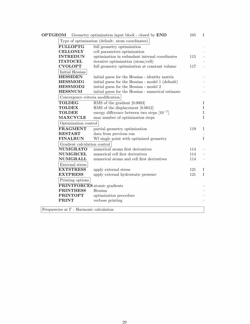
OPTGEOM Geometry optimization input block - closed by END 105 IType of optimization (default: atom coordinates)FULLOPTG full geometry optimization –CELLONLY cell parameters optimization –INTREDUN optimization in redundant internal coordinates 115 –ITATOCEL iterative optimization (atom/cell) –CVOLOPT full geometry optimization at constant volume 117 –Initial HessianHESSIDEN initial guess for the Hessian - identity matrix –HESSMOD1 initial guess for the Hessian - model 1 (default) –HESSMOD2 initial guess for the Hessian - model 2 –HESSNUM initial guess for the Hessian - numerical estimate –Convergence criteria modificationTOLDEG RMS of the gradient [0.0003] ITOLDEX RMS of the displacement [0.0012] ITOLDEE energy difference between two steps [10−7] IMAXCYCLE max number of optimization steps IOptimization controlFRAGMENT partial geometry optimization 119 IRESTART data from previous run –FINALRUN Wf single point with optimized geometry IGradient calculation controlNUMGRATO numerical atoms first derivatives 114 –NUMGRCEL numerical cell first derivatives 114 –NUMGRALL numerical atoms and cell first derivatives 114 –External stressEXTSTRESS apply external stress 121 IEXTPRESS apply external hydrostatic pressure 121 IPrinting optionsPRINTFORCES atomic gradients –PRINTHESS Hessian –PRINTOPT optimization procedure –PRINT verbose printing –

Frequencies at Γ - Harmonic calculation

29

FREQCALC Frequencies at Γ (harmonic calculation) input block - closed by END 127 IANALYSIS –[NOANALYSIS] –DIELISO IDIELTENS IEND[FREQ] –FRAGMENT IINTENS –INTLOC - IR intensities through Wannier functions 134 –[INTPOL] - IR intensities through Berry phase [default] 134 –ISOTOPES 129 I[MODES] –[NOINTENS] –NOMODES –NORMBORN –NOUSESYMM –NUMDERIV IPRESSURE IPRINT –RESTART –SCANMODE ISTEPSIZE ITEMPERAT ITESTFREQ –[USESYMM] –

ANHARM Frequency at Γ (anharmonic calculationinput block - closed by END142 IEND[ANHA] –ISOTOPES modification of atomic mass 143 IKEEPSYMM 44 –NOGUESS 143 –POINTS26 143 –PRINT –TEST[ANHA] –

CONFCNT - Configuration counting and cluster expansion 147

CPHF - Coupled Perturbed Hartree-Fock 145

ELASTCON - Second order elastic constants 149

EOS - Equation of state 145

Geometry input optional keywords

ANGLES

This option prints the angle the AXB, where X is one of the irreducible (that is, non symmetryequivalent) atoms of the unit cell, and A and B belong to its m-th and n-th stars of neighbors.

30

rec variable meaning• ∗ NATIR number of X atoms to be considered; they are the first NATIR in the list of

irreducible atoms (flag ”T” printed) generated by CRYSTAL∗ NSHEL number of stars of neighbors of X to be considered; all the angles AXB,

where A and B belong to the first NSHEL neighbors of X, are printed out

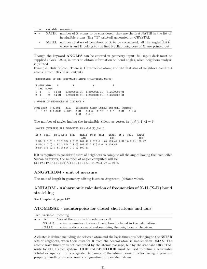
Though the keyword ANGLES can be entered in geometry input, full input deck must besupplied (block 1-2-3), in order to obtain information on bond angles, when neighbors analysisis printed.Example. Bulk Silicon. There is 1 irreducible atom, and the first star of neighbors contain 4atoms: (from CRYSTAL output):

COORDINATES OF THE EQUIVALENT ATOMS (FRACTIONAL UNITS)

N ATOM ATOM Z X Y Z

IRR EQUIV

1 1 1 14 SI 1.250000E-01 1.250000E-01 1.250000E-01

2 1 2 14 SI -1.250000E-01 -1.250000E-01 - 1.250000E-01

- - - - - - - - - - - - - - - - - - - - - - -

N NUMBER OF NEIGHBORS AT DISTANCE R

STAR ATOM N R/ANG R/AU NEIGHBORS (ATOM LABELS AND CELL INDICES)

1 1 SI 4 2.3469 4.4351 2 SI 0 0 0 2 SI 1 0 0 2 SI 0 1 0

2 SI 0 0 1

The number of angles having the irreducible Silicon as vertex is: (4)*(4-1)/2 = 6

ANGLES (DEGREES) ARE INDICATED AS A-X-B(I),I=1,L

at A cell at X at B cell angle at B cell angle at B cell angle

AXB AXB AXB

2 SI( 0 0 0) 1 SI 2 SI( 1 0 0) 109.47 2 SI( 0 1 0) 109.47 2 SI( 0 0 1) 109.47

2 SI( 1 0 0) 1 SI 2 SI( 0 1 0) 109.47 2 SI( 0 0 1) 109.47

2 SI( 0 1 0) 1 SI 2 SI( 0 0 1) 109.47

If it is required to consider 6 stars of neighbors to compute all the angles having the irreducibleSilicon as vertex, the number of angles computed will be:(4+12+12+6+12+24)*(4+12+12+6+12+24-1)/2 = 2415

ANGSTROM - unit of measure

The unit of length in geometry editing is set to Angstrom, (default value).

ANHARM - Anharmonic calculation of frequencies of X-H (X-D) bondstretching

See Chapter 4, page 142.

ATOMBSSE - counterpoise for closed shell atoms and ions

rec variable meaning• ∗ IAT label of the atom in the reference cell

NSTAR maximum number of stars of neighbors included in the calculation.RMAX maximum distance explored searching the neighbors of the atom.

A cluster is defined including the selected atom and the basis functions belonging to the NSTARsets of neighbors, when their distance R from the central atom is smaller than RMAX. Theatomic wave function is not computed by the atomic package, but by the standard CRYSTALroute for 0D, 1 atom system. UHF and SPINLOCK must be used to define a reasonableorbital occupancy. It is suggested to compute the atomic wave function using a programproperly handling the electronic configuration of open shell atoms.

31

Warning. The system is 0D. No reciprocal lattice information is required in the scf input(Section 1.3, page 23).

ATOMDISP

rec variable meaning• ∗ NDISP number of atoms to be displaced

insert NDISP records II• ∗ LB label of the atom to be moved

DX,DY,DZ increments of the coordinates in the primitive cell [A].

Selected atoms are displaced in the primitive cell. The point symmetry of the system may bealtered (default value BREAKSYM, page 34). To displace all the atoms symmetry related,KEEPSYMM must be inserted before ATOMDISP.Increments are in Angstrom, unless otherwise requested (keyword BOHR, FRACTION,page 31). See tests 17, 20, 37.

ATOMINSE

rec variable meaning• ∗ NINS number of atoms to be added

insert NINS records II• ∗ NA conventional atomic number

X,Y,Z coordinates [A] of the inserted atom. Coordinates refer to the primitive cell.

New atoms are added to the primitive cell. Coordinates are in Angstrom, unless otherwiserequested (keyword BOHR, FRACTION, page 31). Remember that the original symmetryof the system is maintained, applying the symmetry operators to the added atoms if thekeyword KEEPSYMM (page 34) was previously entered. The default is BREAKSYM(page 34). Attention should be paid to the neutrality of the cell (see CHARGED, page 62).See tests 16, 35, 36.

ATOMORDE

After processing the standard geometry input, the symmetry equivalent atoms in the referencecell are grouped. They may be reordered, following a chemical bond criterion. This simplifiesthe interpretation of the output when the results of bulk molecular crystals are compared withthose of the isolated molecule. See option MOLECULE (page 46) and MOLSPLIT (page47). No input data are required.For molecular crystals only.

ATOMREMO

rec variable meaning• ∗ NL number of atoms to remove• ∗ LB(L),L=1,NL label of the atoms to remove

Selected atoms, and related basis set, are removed from the primitive cell (see test 16). Avacancy is created in the lattice. The symmetry can be maintained (KEEPSYMM), byremoving all the atoms symmetry-related to the selected one, or reduced (BREAKSYM,default). Attention should be paid to the neutrality of the cell (see CHARGED, page 62).NB. The keyword GHOSTS (basis set input, page 64) allows removal of selected atoms,leaving the related basis set.

32

ATOMROT

rec variable value meaning• ∗ NA 0 all the atoms of the cell are rotated and/or translated

>0 only NA selected atoms are rotated and/or translated.<0 the atom with label |NA| belongs to the molecule to be rotated. The

program selects all the atoms of the molecule on the base of the sum oftheir atomic radii (Table on page 53).

if NA > 0, insert NA data II• ∗ LB(I),I=1,NA label of the atoms to be rotated and/or translated.• ∗ ITR >0 translation performed. The selected NA atoms are translated by -r,

where r is the position of the ITR-th atom. ITR is at the origin afterthe translation.

≤ 0 a general translation is performed. See below.=999 no translation.

IRO > 0 a rotation around a given axis is performed. See below.< 0 a general rotation is performed. See below.=999 no rotation.

if ITR<0 insert II• ∗ X,Y,Z Cartesian components of the translation vector [A]

if ITR=0 insert II• ∗ N1,N2 label of the atoms defining the axis.

DR translation along the axis defined by the atoms N1 and N2, in the di-rection N1 → N2 [A].

if IRO<0 insert II• ∗ A,B,G Euler rotation angles (degree).

IPAR defines the origin of the Cartesian system for the rotation0 the origin is the barycentre of the NAT atoms>0 the origin is the atom of label IPAR

if IRO>0 insert II• ∗ N1,N2 label of the atoms that define the axis for the rotation

ALPHA 6= 0. rotation angle around the N1–N2 axis (degrees)0. the selected atoms are rotated anti-clockwise in order to orientate the

N1–N2 axis parallel to the z axis.

This option allows to rotate and/or translate the specified atoms. When the rotation of amolecule is required (NA < 0), the value of the atomic radii must be checked, in order toobtain a correct definition of the molecule. It is useful to study the conformation of a moleculein a zeolite cavity, or the interaction of a molecule (methane) with a surface (MgO).The translation of the selected group of atoms can be defined in three different ways:

1. Cartesian components of the translation vector (ITR < 0);

2. modulus of the translation vector along an axis defined by two atoms (ITR = 0);

3. sequence number of the atom to be translated to the origin. All the selected atoms aresubjected to the same translation (ITR > 0).

The rotation can be performed in three different ways:

1. by defining the Euler rotation angles α, β, γ and the origin of the rotating system (IRO< 0). The axes of the rotating system are parallel to the axes of the Cartesian referencesystem. (The rotation is given by: RαzRβxRγz, where R are the rotation matrices).

2. by defining the rotation angle α around an axis defined by two atoms A and B. Theorigin is at A, the positive direction A→B.

3. by defining a z’ axis (identified by two atoms A and B). The selected atoms are rotated,in such a way that the A–B z’ axis becomes parallel to the z Cartesian axis. The originis at A and the positive rotation anti clockwise (IRO>0, α=0).

33

The selected atoms are rotated according to the defined rules, the cell orientation and thecartesian reference frame are not modified. The symmetry of the system is checked after therotation, as the new geometry may have a different symmetry.See tests 15, rotation of the NH3 molecule in a zeolite cavity, and 16, rotation of the H2Omolecule in the zeolite cavity.

ATOMSUBS

rec variable meaning• ∗ NSOST number of atoms to be substituted

insert NSOST records II• ∗ LB label of the atom to substitute

NA(LB) conventional atomic number of the new atom

Selected atoms are substituted in the primitive cell (see test 17, 34, 37). The symmetry can bemaintained (KEEPSYMM), by substituting all the atoms symmetry-related to the selectedone, or reduced (BREAKSYM, default). Attention should be paid to the neutrality of thecell: a non-neutral cell will cause an error message, unless allowed by entering the keywordCHARGED, page 62.

ATOMSYMM

The point group associated with each atomic position and the set of symmetry related atomsare printed. No input data are required. This option is useful to find the internal coordinatesto be relaxed when the unit cell is deformed (see ELASTIC, page 38).

BOHR

The keyword BOHR sets the unit of distance to bohr. When the unit of measure is modified,the new convention is active for all subsequent geometry editing.The conversion factor Angstrom/bohr is 0.5291772083 (CODATA 1998). This value can bemodified by entering the keyword BOHRANGS and the desired value in the record following.The keyword BOHRCR98 sets the conversion factor to 0.529177, as in the program CRYS-TAL98.CRYSTAL88 default value was 0.529167).

BOHRANGS

rec variable meaning• ∗ BOHR conversion factor Angstrom/bohr

The conversion factor Angstrom/bohr can be user-defined.In CRYSTAL88 the default value was 0.529167.In CRYSTAL98 the default value was 0.529177.

BOHRCR98

The conversion factor Angstrom/bohr is set to 0.529177, as in CRYSTAL98. No input datarequired.

BREAKSYM

Under control of the BREAKSYM keyword (the default), subsequent modifications of thegeometry are allowed to alter (reduce: the number of symmetry operators cannot be increased)the point-group symmetry. The new group is a subgroup of the original group and is automat-ically obtained by CRYSTAL.

34

The symmetry may be broken by attributing different spin (ATOMSPIN, block34, page 72)to atoms symmetry related by geometry.Example: When a CO molecule is vertically adsorbed on a (001) 3-layer MgO slab, (D4h

symmetry), the symmetry is reduced to C4v, if the BREAKSYM keyword is active. Thesymmetry operators related to the σh plane are removed. However, if KEEPSYMM isactive, then additional atoms will be added to the underside of the slab so as to maintain theσh plane (see page 32, keyword ATOMINSE).

BREAKELAS (for 3D systems only)

This keyword breaks the symmetry of 3D sysems according to a general distortion (3x3 adi-mensional matrix, not necessarily symmetric):

rec variable value meaning• ∗ D11 D12 D13 first row of the matrix.• ∗ D21 D22 D23 second row of the matrix.• ∗ D31 D32 D33 third row of the matrix.

BREAKELAS can be used when the symmetry must be reduced to apply an external stress(see EXTSTRESS, OPTGEOM input block, page 121) not compatible with the present sym-metry.

BREAKELAS reduces the symmetry according to the distortion defined in input, but doesnot perform a distortion of the lattice.

Another possibility is when you compute elastic constants, and you want to fix a referencegeometry with FIXINDEX. If your reference geometry has a symmetry higher than the dis-torted one, then you had to break the symmetry by applying e.g. a tiny elastic distortionwith ELASTIC. By using BREAKELAS you can reduce the symetry without distortion of thelattice.

Example - Geometry optimization of MgO bulk, cubic, with an applied uniaxial stress modi-fying the symmetry of the cell.

TEST11 - MGO BULKCRYSTAL0 0 02254.21212 0. 0. 0.8 0.5 0.5 0.5

BREAKELAS the number of symmops is reduced, from 48 to 160.001 0. 0. the cell has a tetragonal symmetry now0. 0. 0.0. 0. 0.OPTGEOMFULLOPTGEXTSTRESS0.001 0. 0.0. 0. 0.0. 0. 0.ENDOPT

When EXTSTRESS is requested, the code automatically checks if the required distortion ispossible or not (if the symmetry had not been broken properly beforehand, an error messagecomes).

35

CONFCNT - Mapping of CRYSTAL calculations to model Hamilto-nians


CPHF - performs the Coupled Perturbed HF/KS calculation up tothe second order


CLUSTER - a cluster (0D) from a periodic system

The CLUSTER option allows one to cut a finite molecular cluster of atoms from a periodiclattice. The size of the cluster (which is centred on a specified ’seed point’ A) can be controlledeither by including all atoms within a sphere of a given radius centred on A, or by specifyinga maximum number of symmetry-related stars of atoms to be included.The cluster includes the atoms B (belonging to different cells of the direct lattice) satisfyingthe following criteria:

1. those which belong to one of the first N (input data) stars of neighbours of the seed pointof the cluster.

and

2. those at a distance RAB from the seed point which is smaller then RMAX (input datum).

The resulting cluster may not reproduce exactly the desired arrangement of atoms, particularlyin crystals with complex structures such as zeolites, and so it is possible to specify bordermodifications to be made after definition of the core cluster.Specification of the core cluster:

rec variable value meaning• ∗ X, Y, Z coordinates of the centre of the cluster [A] (the seed point)

NST maximum number of stars of neighbours explored in defining the corecluster

RMAX radius of a sphere centred at X,Y,Z containing the atoms of the corecluster

• ∗ NNA 6= 0 print nearest neighbour analysis of cluster atoms (according to a radiuscriterion)

NCN 0 testing of coordination number during hydrogen saturation carried outonly for Si (coordination number 4), Al (4) and O(2)

N N user-defined coordination numbers are to be definedif NNA 6= 0 insert 1 record II

• ∗ RNNA radius of sphere in which to search for neighbours of a given atom inorder to print the nearest neighbour analysis

if NCN 6= 0 insert NCN records II• ∗ L conventional atomic number of atom

MCONN(L) coordination number of the atom with conventional atomic number L.MCONN=0, coordination not tested

Border modification:

36

rec variable value meaning• ∗ NMO number of border atoms to be modified

if NMO > 0 insert NMO records II• ∗ IPAD label of the atom to be modified (cluster sequence)

NVIC number of stars of neighbours of atom IPAD to be added to the clusterIPAR = 0 no hydrogen saturation

6= 0 cluster border saturated with hydrogen atomsBOND bond length Hydrogen-IPAD atom (direction unchanged).

if NMO < 0 insert II• ∗ IMIN label of the first atom to be saturated (cluster sequence)

IMAX label of the last atom to be saturated (cluster sequence)NVIC number of stars of neighbours of each atom to be added to the clusterIPAR = 0 no hydrogen saturation

6= 0 cluster border saturated with hydrogen atomsBOND H-cluster atom bond length (direction unchanged).

The two kinds of possible modification of the core cluster are (a) addition of further stars ofneighbours to specified border atoms, and (b) saturation of the border atoms with hydrogen.This latter option can be essential in minimizing border electric field effects in calculations forcovalently-bonded systems.(Substitution of atoms with hydrogen is obtained by HYDROSUB).The hydrogen saturation procedure is carried out in the following way. First, a coordinationnumber for each atom is assumed (by default 4 for Si, 4 for Al and 2 for O, but these maybe modified in the input deck for any atomic number). The actual number of neighbours ofeach specified border atom is then determined (according to a covalent radius criterion) andcompared with the assumed connectivity. If these two numbers differ, additional neighbours areadded. If these atoms are not neighbours of any other existing cluster atoms, they are convertedto hydrogen, otherwise further atoms are added until the connectivity allows complete hydrogensaturation whilst maintaining correct coordination numbers.The label of the IPAD atoms refers to the generated cluster, not to the original unit cell. Thepreparation of the input thus requires two runs:

1. run using the CLUSTER option with NMO=0, in order to generate the sequence numberof the atoms in the core cluster. The keyword TESTGEOM should be inserted in thegeometry input block. Setting NNA 6= 0 in the input will print a coordination analysis ofall core cluster atoms, including all neighbours within a distance RNNA (which shouldbe set slightly greater than the maximum nearest neighbour bond length). This can beuseful in deciding what border modifications are necessary.

2. run using the CLUSTER option with NMO 6= 0, to perform desired border modifica-tions.

Note that the standard CRYSTAL geometry editing options may also be used to modify thecluster (for example by adding or deleting atoms) placing these keywords after the specificationof the CLUSTER input.Warning. The system is 0D. No reciprocal lattice information is required in the scf input(Section 1.3, page 23). See test 16.

COORPRT

Geometry information is printed: cell parameters, fractional coordinates of all atoms in thereference cell, symmetry operators.A formatted file, ”fort.33” , is written. See Appendix D, page 262. No input data are re-quired. The file ”fort.33” has the right format for the program MOLDEN [116] which can bedownloaded from:www.cmbi.ru.nl/molden/molden.html

37

ELASTCON - Calculation of elastic constants


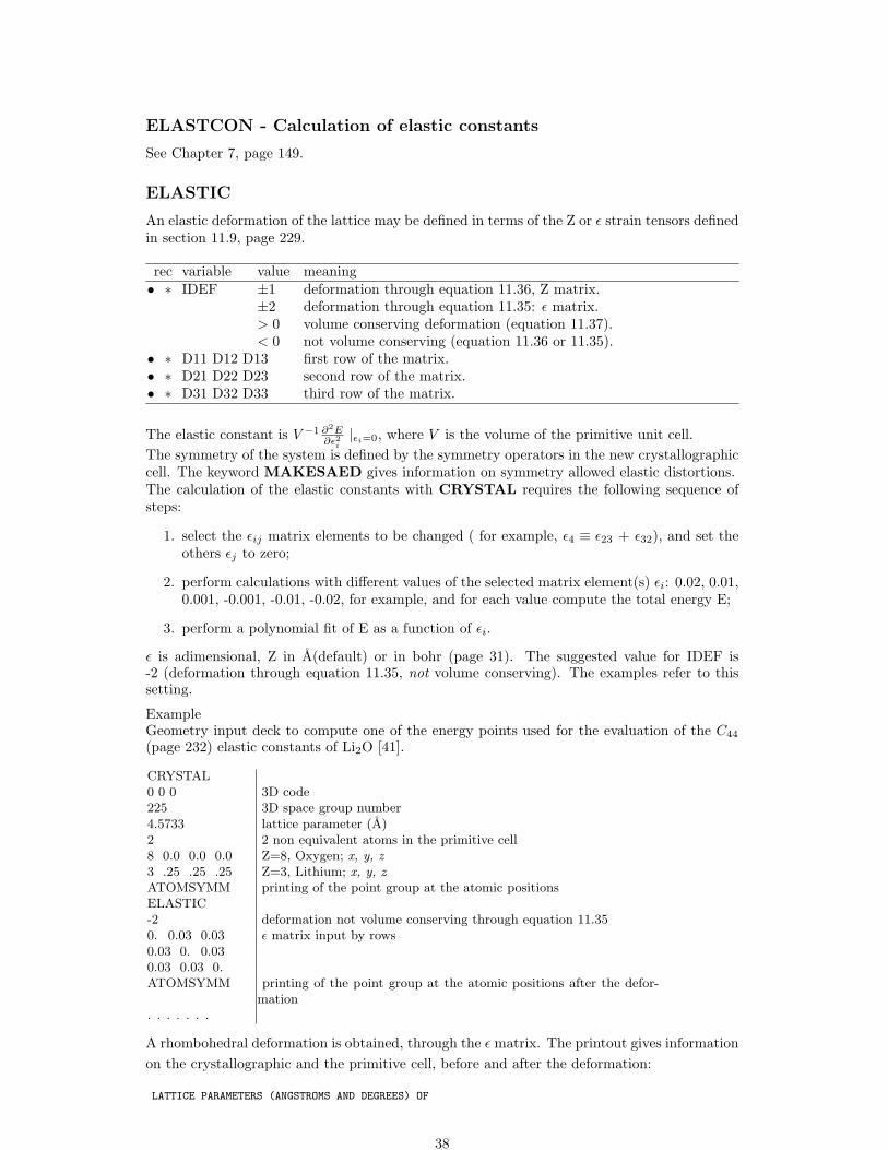
ELASTIC

An elastic deformation of the lattice may be defined in terms of the Z or ε strain tensors definedin section 11.9, page 229.

rec variable value meaning• ∗ IDEF ±1 deformation through equation 11.36, Z matrix.

±2 deformation through equation 11.35: ε matrix.> 0 volume conserving deformation (equation 11.37).< 0 not volume conserving (equation 11.36 or 11.35).

• ∗ D11 D12 D13 first row of the matrix.• ∗ D21 D22 D23 second row of the matrix.• ∗ D31 D32 D33 third row of the matrix.

The elastic constant is V −1 ∂2E∂ε2i

|εi=0, where V is the volume of the primitive unit cell.The symmetry of the system is defined by the symmetry operators in the new crystallographiccell. The keyword MAKESAED gives information on symmetry allowed elastic distortions.The calculation of the elastic constants with CRYSTAL requires the following sequence ofsteps:

1. select the εij matrix elements to be changed ( for example, ε4 ≡ ε23 + ε32), and set theothers εj to zero;

2. perform calculations with different values of the selected matrix element(s) εi: 0.02, 0.01,0.001, -0.001, -0.01, -0.02, for example, and for each value compute the total energy E;

3. perform a polynomial fit of E as a function of εi.

ε is adimensional, Z in A(default) or in bohr (page 31). The suggested value for IDEF is-2 (deformation through equation 11.35, not volume conserving). The examples refer to thissetting.

ExampleGeometry input deck to compute one of the energy points used for the evaluation of the C44

(page 232) elastic constants of Li2O [41].

CRYSTAL0 0 0 3D code225 3D space group number4.5733 lattice parameter (A)2 2 non equivalent atoms in the primitive cell8 0.0 0.0 0.0 Z=8, Oxygen; x, y, z3 .25 .25 .25 Z=3, Lithium; x, y, zATOMSYMM printing of the point group at the atomic positionsELASTIC-2 deformation not volume conserving through equation 11.350. 0.03 0.03 ε matrix input by rows0.03 0. 0.030.03 0.03 0.ATOMSYMM printing of the point group at the atomic positions after the defor-

mation. . . . . . .

A rhombohedral deformation is obtained, through the ε matrix. The printout gives informationon the crystallographic and the primitive cell, before and after the deformation:

LATTICE PARAMETERS (ANGSTROMS AND DEGREES) OF

38

(1) ORIGINAL PRIMITIVE CELL

(2) ORIGINAL CRYSTALLOGRAPHIC CELL

(3) DEFORMED PRIMITIVE CELL

(4) DEFORMED CRYSTALLOGRAPHIC CELL

A B C ALPHA BETA GAMMA VOLUME

(1) 3.233811 3.233811 3.233811 60.000000 60.000000 60.000000 23.912726

(2) 4.573300 4.573300 4.573300 90.000000 90.000000 90.000000 95.650903

(3) 3.333650 3.333650 3.333650 56.130247 56.130247 56.130247 23.849453

(4) 4.577414 4.577414 4.577414 86.514808 86.514808 86.514808 95.397811

After the deformation of the lattice, the point symmetry of the Li atoms is C3v, where the C3

axis is along the (x,x,x) direction. The Li atoms can be shifted along the principal diagonal,direction (x,x,x) of the primitive cell without altering the point symmetry, as shown by theprinting of the point group symmetry obtained by the keyword ATOMSYMM (page 34).See test20 for complete input deck, including shift of the Li atoms.See test38 (KCoF3).

END

Terminate processing of block 1, geometry definition, input. Execution continues. Subsequentinput records are processed, if required.Processing of geometry input block stops when the first three characters of the string are”END”. Any character can follow: ENDGEOM, ENDGINP, etc etc.

EOS - Equation of state

E vs V curves can be computed automatically by specifying the keyword EOS in input block1 (geometry). EOS must be the last keyword in geometry input.

. . . geometry input . . . .

EOS

END[EOS] close EOS input block

END close geometry input block

EOS input block admits several options (subkeywords), and terminates with keyword END(or END[EOS], END[—]: the first three characters only are processed).

A constant volume geometry optimization is performed for each point and results are thenfitted to most common equation of states (e.g. Birch-Murnagham 3rd-order). The constantvolume geometry optimization can be only performed in fractional coordinates.

Note that the initial geometry must be fully relaxed.

Work is in progress to extend this scheme to E vs P calculations

Keywords, options, and defaults

A default value is chosen for all computational parameters.SCF energy convergence threshold is set to 10−8. To modify it, see keyword TOLDEE ininput block 3, page 102.

Optional keywords are (in any order):

39


• A smRANGE keyword to specify the range of volumes in the E(V) curve∗ VMIN minimum (compression) variation of the initial volume [default =

0.92]∗ VMAX maximum (expansion) variation of the initial volume [default = 1.08]∗ NPOINTS number of points in the selected range [default = 10]

The interval is specified as the minimum (compression) and maximum (expansion) variation ofthe volume of the initial geometry. The set of volumes is then defined according to the numberof points in the selected range. For instance, to set the default values:

...

EOS

RANGE

0.92 1.08 10

END[EOS]

...

corresponds to 10 points between 0.92*Vini and 1.08*Vini, where Vini is the volume of theinitial geometry given as input (assumed to be the fully optimized structure) or as obtainedafter a preliminary geometry optimization.Note that the initial E-V value is always included in the final data for fitting (i.e. 11 points inthe example above).


• A PRINT This option turns on a higher level of diagnostic printing and willgenerally not be necessary for the typical user. LPRINT(250) isset equal to 1 with this option. Fitting of the E(V) points is alsoperformed for increasing set of points from 3 to the maximum num-ber of points. (default is minimal printing and no additional linesshould exist)

• A RESTART Allows for a RESTART using file EOSINFO.DAT from a previousrun.

• A PREOPTGEOM A preliminary geometry optimization of cell and atomic positionsis performed before starting the E(V) curve calculation.

Geometry optimization is performed at convergence criteria tighter than the ones given inOPTGEOM. Some values can be modified by inserting the following keywords:

• A TOLDEG EOS default [0.00006] - see OPTGEOM, page 110• A TOLDEX EOS default [0.00012] - see OPTGEOM, page 110• A TOLDEE EOS default [8] - see OPTGEOM, page 110• A MAXCYCLE see OPTGEOM, page 113• A NOTRUSTR see OPTGEOM, page 111• A TRUSTRADIUS see OPTGEOM, page 111• A MAXTRADIUS see OPTGEOM, page 111

Important remarks

• The structure given as input should be fully optimized. Note that the same tighterconvergence criteria as in the calculation of the E vs V curve must be used as well as

40

the FINALRUN=4 option.

• Integrals classification is done on the input geometry. Therefore, initial geometry mustbe the equilibrium structure to avoid slightly shifted curves with respect to the trueminimum.

EXTPRT

A formatted input deck with explicit structural/symmetry information is written in file”fort.34”. If the keyword is entered many times, the data are overwritten. The last geom-etry is recorded. The file may be used as crystal geometry input to CRYSTAL through theEXTERNAL keyword.For instance, to enter the final optimized geometry, or a geometry obtained by editing opera-tions who modified the original space group or periodicity.When geometry optimization is performed, the name of the file is ”optc(a)xxx”, being xxx thenumber of the cycle, and it is automatically written at each cycle.Please refer to the standard script for running CRYSTAL09 to handle input/output file names.See Appendix D, page 258.

No input data are required.

FIELD - Electric field along a periodic direction

rec variable value meaning• ∗ E0MAX electric field intensity E0 (in atomic units)• ∗ DIRE(I),I=1,3 crystallographic (Miller) indices of the plane perpendicular to the elec-

tric field• ∗ SMFACT supercell expansion factor∗ IORTO 0 non-orthogonal supercell

1 orthogonal supercell• ∗ MUL number of term in Fourier expansion for triangular electric potential∗ ISYM +1 triangular potential is symmetric with respect to the z = 0 plane

−1 triangular potential is anti-symmetric with respect to the z = 0 plane

This option can be used with polymers, slabs and crystals and permits to apply an electricfield along a periodic direction of the system.The effect of a periodic electric field ( ~E) is taken into account according to a perturbationscheme. The Hamiltonian (Fock or Kohn-Sham) can be written as::

H = H0 + H1( ~E) (2.1)

where H0 is the unperturbed Hamiltonian and H1( ~E) the electric potential term.During the SCF procedure crystalline orbitals are relaxed under the effect of the field, leadingto a perturbed wave function and charge density.

The applied electric field has a square-wave form, that corresponds to a triangular (”sawtooth”)electric potential.Due to the form of the potential, a single unit cell must contain both positive and negativepart of the square wave electric field. Then, in order to maintain translational invariance of thesystem a new, expanded, unit cell is automatically created by adopting a supercell approach(see keywords SUPERCEL/SUPERCON, page 56).This procedure consists in two automatic steps: the re-orientation of the c lattice parameter

41

along the chosen field direction and the multiplication of this lattice vector according to thesupercell expansion factor (~C=SMFACT·~c, see fig. 2.1). By varying this parameter is possibleto control the period of the electric potential and therefore the length of the constant regionof the electric field.

Figure 2.1: Triangular electric potential (”sawtooth”) in a supercell with SMFACT = 4.

Then, for computational reasons, an automatic rotation of the crystal in the cartesian referencesystem is performed by aligning ~C (and therefore ~E) along the z cartesian direction (seekeyword ROTCRY, page 54). After these transformations the field is along the z direction,and the perturbation H1( ~E) takes the form:

H±1 (Ez) = V (z) = −qE0 · f±(z) (2.2)

where the f+ (f−) function is expanded as a Fourier series and is chosen according to thesymmetry of the supercell in the direction of the applied field as follows:

f+(z) =2Cπ2

+∞∑k=0

1(2k + 1)2

cos(

2π(2k + 1)zC

)(2.3)

f−(z) =2Cπ2

+∞∑k=0

(−1)k

(2k + 1)2sin(

2π(2k + 1)zC

)(2.4)

1. In order to evaluate the dielectric constant of a material in the direction of the appliedfield it is necessary to run a PROPERTIES calculation with the keyword DIEL (see page160). In this way the perturbed wave function is used for the calculation of ε, followinga macroscopic average scheme, as described in references [54], [32].

2. The field is along the z axis for 3D-crystal calculations; it is along the x for 1D-polymerand 2D-slab calculations.

3. In calculations of the dielectric constant, more accurate results can be achieved by in-creasing the SMFACT value. This will lead to systems characterized by a high numberof atoms with large computational costs. The option IORTO = 0 allows to considernon-orthogonal supercells, characterized by the same dielectric properties of orthogonalcells, but with a lower number of atoms.

4. In 3D-crystals, the electric potential takes a triangular form to maintain translationalsymmetry and electric neutrality of cell. The symmetry of triangular potential has twooptions:

a) ISYM=+1, triangular potential is symmetric with respect to the center of the su-percell, along the z axis. Use this option if there is a symmetry plane orthogonal tothe z axis.

b) ISYM=−1, triangular potential is anti-symmetric. This option can be used whenthe supercell does not have a symmetry plane orthogonal to z axis.

42

Figure 2.2: Left: symmetric triangular electric potential (ISIM = 1). Right anti-symmetrictriangular electric potential (ISYM=-1).

5. MUL, the number of terms in the Fourier expansion, can take values between 1 and 60.

MUL=40 is sufficient to adequately reproduce the triangular shape of the potential.

6. High E0MAX values are inconsistent with perturbation method, the choice of E0MAXdepends on the dielectric susceptibility of the system and on the gap width. For small gapcases, use of eigenvalue level shifting technique is recommended (keyword LEVSHIFT,page 92).

7. When an external field is applied, the system can become conducting during the SCFprocedure. In order to avoid convergence problems, it is advisable to set the shrinkingfactor of the Gilat net ISP equal to 2× IS, where IS is the Monkhorst net shrinking factor(see SCF input, page 97).

Conversion factors for electric field:1 AU = 1.71527E+07 ESU·CM−2 = 5.72152E+01 C ·M−2 = 5.14226E+11 V·M−1

FIELDCON - Electric field along non-periodic direction

rec variable meaning• ∗ E(I),I=N,3 field components along x,y,z directions

For a brief theoretical introduction see keyword FIELD.This option can be used with molecules, polymers, slabs and permits to apply an electric fieldalong a non-periodic direction of the system.

1. For molecules (N=1) three components of the field must be supplied, as the field can bedirected along any direction.

2. For polymers (N=2) two components (y,z) of the field must be defined; the x componentof the field must be zero because the default orientation of polymers is along the x axis.

3. For slabs (N=3) just one component (z) of the field have to be defined; the x,y componentsmust be zero because the default orientation of slabs in is in x-y plan.

Conversion factors for electric field:1 AU = 1.71527E+07 ESU·CM−2 = 5.72152E+01 C ·M−2 = 5.14226E+11 V·M−1

This option can evaluate the dielectric response of the molecule, polymer or slab in a directionof non periodicity (see option FIELD for a field along a periodicity direction).

43

Consider the following expansion of the total energy of the system as a function of the appliedfield:

E(F0) = E0 − µF0 −12!αF 2

0 −(1)3!βF 3

0 −14!γF 4

0 − · · · (2.5)

By fitting the E vs F0 data the µ, α, β and γ values can be derived. Seehttp://www.crystal.unito.it → tutorials → Static dielectric constants..

FINDSYM

Geometry information is written in file FINDSYM.DAT, according to the input format of theprogram FINDSYM.

http://stokes.byu.edu/findsym.html

FINDSYM: Identify the space group of a crystal, given the positions of the atoms in a unitcell. When geometry editing modifies the basic input space group, the symmetry of the systemis identified by the symmetry operators only. The program FINDSYM allows identification ofthe space group.

FRACTION

The keyword FRACTION means input coordinates given as fraction of the lattice parameterin subsequent input, along the direction of translational symmetry:

x,y,z crystals (3D)x,y slabs (2D; z in Angstrom or bohr)x polymers (1D; y,z in Angstrom or bohr)

no action for 0D. When the unit of measure is modified, the new convention is active for allsubsequent geometry editing.

FREQCALC - Harmonic frequencies at Γ


HYDROSUB - substitution with hydrogen atoms

rec variable meaning• ∗ NSOST number of atoms to be substituted with hydrogen

insert NSOST records II• ∗ LA label of the atom to substitute

LB label of the atom linked to LABH bond length B-Hydrogen

Selected atoms are substituted with hydrogens, and the bond length is modified. To be usedafter CLUSTER.

KEEPSYMM

In any subsequent editing of the geometry, the program will endeavour to maintain the numberof symmetry operators, by requiring that atoms which are symmetry related remain so aftergeometry editing (keywords: ATOMSUBS, ATOMINSE, ATOMDISP, ATOMREMO)or the basis set (keywords CHEMOD, GHOSTS).

44

Example: When a CO molecule is vertically adsorbed on a (001) 3-layer MgO slab, (D4h

symmetry) (see page 32, keyword ATOMINSE), the symmetry is reduced to C4v, if theBREAKSYM keyword is active. The symmetry operators related to the σh plane are re-moved. However, if KEEPSYMM is active, then additional atoms will be added to theunderside of the slab so as to maintain the σh plane.

MAKESAED

Symmetry allowed elastic distortions are printed. No input data required.

MODISYMM

rec variable meaning• ∗ N number of atoms to be attached a flag• ∗ LA,LF(LA),L=1,N atom labels and flags (n couples of integers in 1 record).

The point symmetry of the lattice is lowered by attributing a different ”flag” to atoms relatedby geometrical symmetry. The symmetry operators linking the two atoms are removed and thenew symmetry of the system is analyzed. For instance, when studying spin-polarized systems, itmay be necessary to apply different spins to atoms which are related by geometrical symmetry.

MOLDRAW

The last version of the program MOLDRAW reads crystal standard output, and can generatea movie from an optimization run. See:

http://www.moldraw.unito.it .

MOLEBSSE - counterpoise for molecular crystals

rec variable meaning• ∗ NMOL number of molecules to be isolatedII insert NMOL records II• ∗ ISEED label of one atom in the n-th molecule

J,K,L integer coordinates (direct lattice) of the primitive cell containing the ISEED

atom• ∗ NSTAR maximum number of stars of neighbours included in the calculation

RMAX maximum distance explored searching the neighbours of the atoms belongingto the molecule(s)

The counterpoise method [17] is applied to correct the Basis Set Superposition Error in molecu-lar crystals. A molecular calculation is performed, with a basis set including the basis functionsof the selected molecules and the neighbouring atoms. The program automatically finds allthe atoms of the molecule(s) containing atom(s) ISEED (keyword MOLECULE, page 46).The molecule is reconstructed on the basis of the covalent radii reported in Table on page 53.They can be modified by running the option RAYCOV, if the reconstruction of the moleculefails. The radius of the hydrogen atom is very critical when intermolecular hydrogen bondsare present.All the functions of the neighbouring atoms in the crystal are added to the basis set of theselected molecule(s) such that both the following criteria are obeyed:

1. the atom is within a distance R lower than RMAX from at least one atom in the molecule

and

45

2. the atom is within the NSTAR-th nearest neighbours of at least one atom in the molecule.

For molecular crystals only.

Warning Do not use with ECP

Warning. The system obtained is 0D. No reciprocal lattice information is required in the scfinput (Section 1.3, page 23). See test 19.

MOLECULE - Extraction of n molecules from a molecular crystal

rec variable meaning• ∗ NMOL number of molecules to be isolatedII insert NMOL records II• ∗ ISEED label of one atom in the nth molecule

J,K,L integer coordinates (direct lattice) of the primitive cell containing theISEED atom

The option MOLECULE isolates one (or more) molecules from a molecular crystal on thebasis of chemical connectivity, defined by the sum of the covalent radii (Table on page 53).The covalent radii can be modified by running the option RAYCOV, if the reconstruction ofthe molecule fails. The covalent radius of the hydrogen atom is very critical when intermolecularhydrogen bonds are present.The input order of the atoms (atoms symmetry related are grouped) is modified, accordingto the chemical connectivity. The same order of the atoms in the bulk crystal is obtained byentering the keyword ATOMORDE (see Section 2.1, page 32). The total number of electronsattributed to the molecule is the sum of the shell charges attributed in the basis set input (inputblock 2, Section 1.2, page 19) to the atoms selected for the molecule.The keyword GAUSS98, entered in input block 2 (basis set input), writes an input deck torun Gaussian 98 (see page 64)

For molecular crystals only.

Warning. The system is 0D. No reciprocal lattice information is required in the scf input(Section 1.3, page 23).Test 18 - Oxalic acid. In the 3D unit cell there are four water and two oxalic acid molecules.The input of test 18 refers to a cluster containing a central oxalic acid molecule surrounded byfour water molecules.

MOLEXP - Variation of lattice parameters at constant symmetryand molecular geometry

rec variable meaning• ∗ δa,[δb],[δc], increments of the minimal set of crystallographic cell parameters:

[δα],[δβ] translation vectors length [Angstrom],[δγ] crystallographic angles (degrees)

The cell parameters (the minimum set, see page 16) are modified, according to the incrementsgiven in input. The volume of the cell is then modified. The symmetry of the lattice and thegeometry (bond lengths and bond angles) of the molecules within the cell is kept. The fractionalcoordinates of the barycentre of the molecules are kept constant, the cartesian coordinatesredefined according to the modification of the lattice parameters. Optimization of the geometrywith reference to the compactness of the lattice is allowed, keeping constant the geometry ofthe molecules. When there are very short hydrogen bonds linking the molecules in the lattice,

46

it may be necessary a modification of the atomic radii to allow proper identification of themolecules (see option RAYCOV, page 53)

MOLSPLIT - Periodic lattice of non-interacting molecules

In order to compare bulk and molecular properties, it can be useful to build a density ma-trix as a superposition of the density matrices of the isolated molecules, arranged in the samegeometry as in the crystal. The keyword MOLSPLIT (no additional input required) per-forms an expansion of the lattice, in such a way that the molecules of the crystal are at an”infinite” distance from each other. The crystal coordinates are scaled so that the distancesinside the molecule are fixed, and the distances among the molecules are expanded by a factor100, to avoid molecule-molecule interactions. The 3D translational symmetry is not changed.Reciprocal lattice information is required in the scf input (Section 1.3, page 23).A standard wave function calculation of the expanded crystal is performed. The densitymatrix refers to the non-interacting subsystems. Before running properties, the latticeis automatically contracted to the bulk situation given in input. If a charge density orelectrostatic potential map is computed (ECHG, POTM options), it corresponds to thesuperposition of the charge densities of the isolated molecules in the bulk geometry.

This option must be used only for molecular crystals only (no charged fragments).

Warning: the DFT grid is not designed for the expanded lattice yet. Large memory allocationmay be necessary.

See test 21.

NANOTUBE - Building a nanotube from a slab

Nanotubes are cylindrical structures, periodic along one direction. They are therefore charac-terised by a single lattice vector. However, in order to study their symmetry and orientation,it is easier to start from a 2D lattice where the additional periodicity becomes the cylinderperiod. This 2D periodic flat structure will be referred in the following, as the nanotube flatlattice.In this flat lattice, 3 vectors are important for the structure description: the rolling vector, ~R,the longitudinal vector, ~L and the helical vector, ~H.

• The rolling vector, ~R = n1 ~a1+n2 ~a2 (where ~a1 and ~a2 are the slab cell vectors), is sufficientto completely define a nanotube. It is used in the literature to characterise the systems(for example the (4,3) nanotube is a nanotube with a rolling vector ~R = 4 ~a1+3 ~a2). In theflat nanotube lattice, ~R is a nanotube unit cell vector. Once the nanotube wrapped, therolling vector becomes a circle normal to the cylinder axis; its norm corresponds to thecylinder perimeter. If ~R passes N times through the lattice nodes, a N -order rotationalaxis will exist along the corresponding nanotube axis.

• The longitudinal vector, ~L = l1 ~a1 + l2 ~a2, is the shortest lattice vector normal to ~R. Inthe nanotube, it becomes the 1D lattice parameter and gives the 1D periodicity alongthe tube axis.

• The helical vector, ~H = h1 ~a1+h2 ~a2, is a lattice vector defining with ~R an area which is Ntimes the area of the unit cell of the flat slab. It satisfies, then, the following relationship

S(~R, ~H)S( ~a1, ~a2)

= |n1h2 − n2h1| = N (2.6)

47

where S(~vi, ~vj) is the surface defined by the ~vi and ~vj vectors. The helical vector defines acorrespondence between a translation in the flat slab and a roto-translation in the curvedsurface; ~H has a rotational component along the circumference vector and a translationalcomponent along the lattice parameter.

The direct product between the rotational and roto-translational operations generates the fullsymmetry of the nanotube.The three vectors listed previously are represented in figure 2.3 for graphene; the examplerefers to the construction of a (4,2) single-walled carbon nanotube (SWCNT).

Figure 2.3: Building the (4,2) SWCNT from graphene.

Further information about the implemented method, the computational costs and the symme-try features of nanotubes are found in Ref. [31] and [132, 7].

rec variable meaning• ∗ n1, n2 components of the roll-up-vector of the nanotube in the slab unit

cell basis. The roll-up-vector, whose length corresponds to the tubecircumference, is expressed as a linear combination of the unit cellvectors of the slab before rolling up, n1 and n2 being integer coeffi-cients.

The convention adopted in CRYSTAL is n1 ≥ n2. In cases when n2 is required to be largerthan n1, it is sufficient to exchange the x and y coordinates of the reference 2D slab.NANOTUBE can be used with the following 2D systems:

• square and hexagonal lattices: any (n1, n2) combination

• rectangular lattices: any n1, n2 = 0

• rhombohedral lattices: n2 = ±n1

In the other cases, the existence of a lattice vector perpendicular to ~R (so the 1D periodicityalong the tube axis) is not guaranteed.The orthogonality condition between ~R and ~L provides the following equation:

~L · ~R = (l1 ~a1 + l2 ~a2) · (n1 ~a1 + n2 ~a2) = n1l1| ~a1|2 + n2l2| ~a2|2 + (n1l2 + n2l1)| ~a1|| ~a2|cos(γ) = 0(2.7)

48

γ being the angle between ~a1 and ~a2. From Equation 2.7 one obtains:

l1l2

= −n2|a2|2 + n1|a1||a2|cos(γ)n1|a1|2 + n2|a1||a2|cos(γ)

(2.8)

If the right term is divided and multiplied by |a2|2, one obtains

l1l2

= − n2 + n1aqcos(γ)aq(n1aq + n2cos(γ))

(2.9)

with aq = |a1||a2| .

The above equation cannot be satisfied for any ( ~a1, ~a2,cos(γ)) combination. This observationis based on the fact that, as l1 and l2 are integers, l1

l2is a rational number, whereas, in general,

cos(γ) and aq are real numbers. In the following the five 2D Bravais lattices are consideredseparately, in order to show which conditions satisfy the periodicity along the tube axis andwhich do not.

• Hexagonal lattice: ~a1 = ~a2, cos(γ) = ±1/2. Equation 2.9 becomes:

l1l2

= −n2 + n1/2n1 + n2/2

= −2n2 + n1

2n1 + n2(2.10)

Any roll-up vector is possible.

• Square lattice: ~a1 = ~a2, cos(γ) = 0.

l1l2

= −n2

n1(2.11)

Any roll-up vector is possible.

• Rectangular lattice: ~a1 6= ~a2, cos(γ) = 0.

l1l2

= −n2|a2|2

n1|a1|2(2.12)

In this case the right term corresponds to a rational number either if |a1| = n|a2|, withn being a rational number, or if n2=0. More generally, for rectangular lattices, theperiodicity along the tube axis is always satisfied for (n, 0) and (0, n) roll-up vectors.

• Rhombohedral (centred rectangular) lattice: ~a1 = ~a2, any cos(γ).

l1l2

= −n2 + n1cos(γ)n1 + n2cos(γ)

(2.13)

The right term provides a rational number only when n1 = n2 or n1 = −n2, so thatEquation 2.13 becomes:

l1l2

= −n1[1 + cos(γ)]n1[1 + cos(γ)]

= −1l1l2

=n1[1− cos(γ)]n1[1− cos(γ)]

= 1 (2.14)

• Oblique lattice: ~a1 6= ~a2, any cos(γ). Equation 2.9 remains as such, and the right termis always an irrational number.

When the above conditions are not satisfied, however, it is possible to manipulate the geometryof the starting slab and force it to assume a suitable form, by building supercells or with minormodifications to the cell parameters.

49

Note that, in cases of hexagonal lattices, the standard convention adopted in CRYSTAL con-siders the reference flat lattice cell vectors forming a 120 angle. In the carbon nanotubeliterature, however, the rolling indices refer to a 60 angle. For this reason, the same inputcan be obtained with the following choices, where the (6,3) indices in the 60 unit cell become(9,3) in the 120 option:

Example I: (6,3) SWCNT from graphene, 60 degrees

SLAB

1

2.47 2.47 60.000

2

6 0.33333333333 0.33333333333 0.000

6 -0.33333333333 -0.33333333333 0.000

NANOTUBE

6 3

Example II: (6,3) SWCNT from graphene, default choice

SLAB

77

2.47

1

6 0.333333 0.666667 0.000000

NANOTUBE

9 3

In order to avoid ambiguity in the choice of the carbon nanotubes indices, use the SWCNT(page 50) keyword.

SWCNT - Building a nanotube from an hexagonal slab (60 unit cellchoice)

rec variable meaning• ∗ n1, n2 Only for hexagonal cells. Same as NANOTUBE keyword but the

components of the rolling vector refer to a 60 hexagonal cell.vspace0.3cm

Example: (6,3) SWCNT from graphene

SLAB

77

2.47

1

6 0.333333 0.666667 0.000000

SWCNT

6 3

See NANOTUBE (page 47) for further details.

Nanotube rebuild: build a nanotube starting from the structure ofanother one, with same directions but a different radius.

Two restart keywords, NANORE and SWCNTRE, allow to build a (n1, n2) nanotube by start-ing from the structure of another one (a previously (nold1, nold2) optimised one, read from filefort.35). The ”old” nanotube is unrolled and re-rolled according to a ”new” ~R vector, withminor modifications to the structure. The rolling direction of the two tubes must be the same.

It is particularly helpful for the geometry optimisation of inorganic nanotubes (thick slabs,large systems, the geometry of the tubes is very different from the one of the slab), as thenumber of optimisation steps is reduced (see Ref. [33] for documentation of computationalgain).

50

NANORE

To be used for tubes built with NANOTUBE (page 47).

rec variable meaning• ∗ nold1, nold2 Nanotube rebuild: indices of the starting nanotube.∗ n1, n2 New indices of the rolling vector.

Consider, for example, the (8,8) and the (10,10) carbon nanotubes (built with NANOTUBE,indices refer to the 120 unit cell choice). We have optimised the structure of the former, andwe want to build the latter starting from its geometry. With NANORE the (8,8) nanotube isunrolled and re-rolled as (10,10). In order to do this, the information on geometry of both thestarting slab (graphene) and the (8,8) nanotube is required. The first one is given in input (orread with EXTERNAL from file fort.34), the second one is read with an EXTERNAL strategyfrom file fort.35. The input syntax is then:

SLAB

77

2.47

1

6 0.333333 0.666667 0.000000

NANORE

8 8

10 10

For nanotubes built with SWCNT (page 50) see SWCNTRE (page 51).

SWCNTRE

It is the same as NANORE, with the same input syntax, but in for hexagonal lattices with 60

unit cell reference (see SWCNT, page 50).

rec variable meaning• ∗ nold1, nold2 Nanotube rebuild: indices of the starting nanotube.∗ n1, n2 New indices of the rolling vector.

NANOJMOL - Graphical visualisation of nanotubes with Jmol

A file named NANOJMOL.DAT containing the nanotube structure is generated. This file canbe directly used by the 3D structure viewer Jmol (www.jmol.org). This keyword must appearin the geometry block before all the keywords related to nanotube construction.

NEIGHBOR/NEIGHPRT

rec variable meaning• ∗ INEIGH number of neighbours of each non-equivalent atom to be printed

The option is active when analyzing the crystal structure (bond lengths and bond angles) andwhen printing the bond populations following Mulliken analysis. Full input deck must be given(block 1-2-3),in order to obtain neighbors analysis of all the non-equivalent atomsFor each non-equivalent atom information on the first INEIGH neighbours is printed: number,type, distance, position (indices of the direct lattice cell).Warning: the neighbors analysis is performed after the symmetry analysis and the screeningof the integrals. If very soft tolerances for the integrals screening are given in input, it mayhappen that the information is not given for all the neighbors requested, as their are not takeninto account when truncation criteria are applied.

51

NOSHIFT

It may be used before SUPERCEL keyword. It avoids shift of the origin in order to minimizethe number of symmetry operators with finite translation component. No input data arerequired.

OPTGEOM - Full geometry optimization


ORIGIN

The origin is moved to minimize the number of symmetry operators with finite translationcomponents. Suggested before cutting a slab from a 3D structure (option SLABCUT, page55). No input data are required.

PARAMPRT - printing of parametrized dimensions

The parameters controlling the dimensions of the static allocation arrays of the program areprinted. No input data are required.

POINTCHG

rec variable meaning• ∗ NCH number of point charges to be added

insert NCH records II• ∗ X,Y,Z,QC cartesian coordinates [A], charge(au). Coordinates refer to the primitive cell.

Dummy atoms with formal atomic number 93, mass zero, nuclear charge as given in input (filePOINTCHG.INP), are added to the primitive cell. Data are read in free format.

record type of data content1 1 integer N, number of point charges2..2+N-1 4 real x y z charge

Coordinates are in Angstrom, unless otherwise requested (keyword BOHR, page 31). Chargesare net charges (1 electron = -1). The symmetry of the system must be removed by the keywordSYMMREMO.As point charges are formally considered as ”atoms”, they must be the last addition of centresto the system.No electron charge should be attributed to those atoms in basis set input (no atomic wavefunction calculation is possible). The default basis set defined by the program is a single sgaussian, with exponent 100000.Attention should be paid to the neutrality of the cell. If the absolute value of the sum of thecharges is less than 10−3, the value of the charges is ”normalized” to obtain 0.The data given in input are printed. To obtain printing of coordinates and neighbour analysisof the dummy atoms in geometry output, insert the keyword PRINTCHG.

Not compatible with: OPTGEOM, FREQCALC, ANHARM, ELASTCON, EOS,FIELD, FIELDCON, NOBIPOLA.

PRIMITIV

Some properties (XFAC, EMDL, EMDP, PROF) input the oblique coordinates of the kpoints in the reciprocal lattice with reference to the conventional cell, though the computationrefers to the primitive one. This option allows entering directly the data with reference to theprimitive cell. The transformation matrix from primitive to crystallographic (Appendix A.5,page 244) is set to the identity. No effect on the CPU time: CRYSTAL always refers to theprimitive cell. No input data are required.

52

PRINTCHG

Coordinates of the dummy atoms inserted after the keyword POINTCHG are printed ingeometry output, basis set output, neighbor analysis. No input data required.

PRINTOUT - Setting of printing environment

Extended printout can be obtained by entering selected keywords in a printing environmentbeginning with the keyword PRINTOUT and ending with the keyword END. The possiblekeywords are found in the fifth column of the table on page 256.Extended printing request can be entered in any input block. Printing requests are not trans-ferred from wave function to properties calculation.See Appendix C, page 254.

PRSYMDIR

Printing of the so-called symmetry allowed directions adopted in the geometry optimization.The printing is done after the neighbor analysis, before computing the wave function. Fullinput must be supplied (3 blocks). Test run allowed with the keyword TESTPDIM.No input data required.

PURIFY

This cleans up the atomic positions so that they are fully consistent with the group (to withinmachine rounding error). Atomic position are automatically redefined after basic geometryinput. No input data are required.

RAYCOV - covalent radii modification

rec variable meaning• ∗ NCOV number of atoms for which the covalent radius is redefined

insert NCOV records II• ∗ NAT atomic number (0 ≤NAT ≤ 92)

RAY covalent radius of the atom with atomic number NAT ([A], default,or bohr, if the keyword BOHR precedes in the deck)

The option RAYCOV allows modification of the covalent radius default value for a givenatom.

Table of covalent radii (Angstrom)

H He

0.68 1.47

--------- -----------------------------

Li Be B C N O F Ne

1.65 1.18 0.93 0.81 0.78 0.78 0.76 1.68

--------- -----------------------------


2.01 1.57 1.50 1.23 1.15 1.09 1.05 1.97

-----------------------------------------------------------------------------------------

K Ca Sc Ti V Cr Mn Fe Co Ni Cu Zn Ga Ge As Se Br Kr

2.31 2.07 1.68 1.47 1.41 1.47 1.47 1.47 1.41 1.41 1.41 1.41 1.36 1.31 1.21 1.21 1.21 2.10

-----------------------------------------------------------------------------------------

Rb Sr Y Zr Ni Mo Tc Ru Rh Pd Ag Cd In Sn Sb Te I Xe

2.31 2.10 1.94 1.60 1.52 1.52 1.42 1.36 1.42 1.47 1.68 1.62 1.62 1.52 1.52 1.47 1.47 2.66

-----------------------------------------------------------------------------------------

Cs Ba La Hf Ta W Re Os Ir Pt Au Hg Tl Pb Bi Po At Rn

2.73 2.10 1.94 1.63 1.63 1.63 1.63 1.63 1.63 1.63 1.63 1.63 1.99 1.89 1.68 1.42 1.42 1.62

-----------------------------------------------------------------------------------------

The choice of the covalent radius of hydrogen may be very critical when extracting a moleculefrom a hydrogen bonded molecular crystal. See test 15.

53

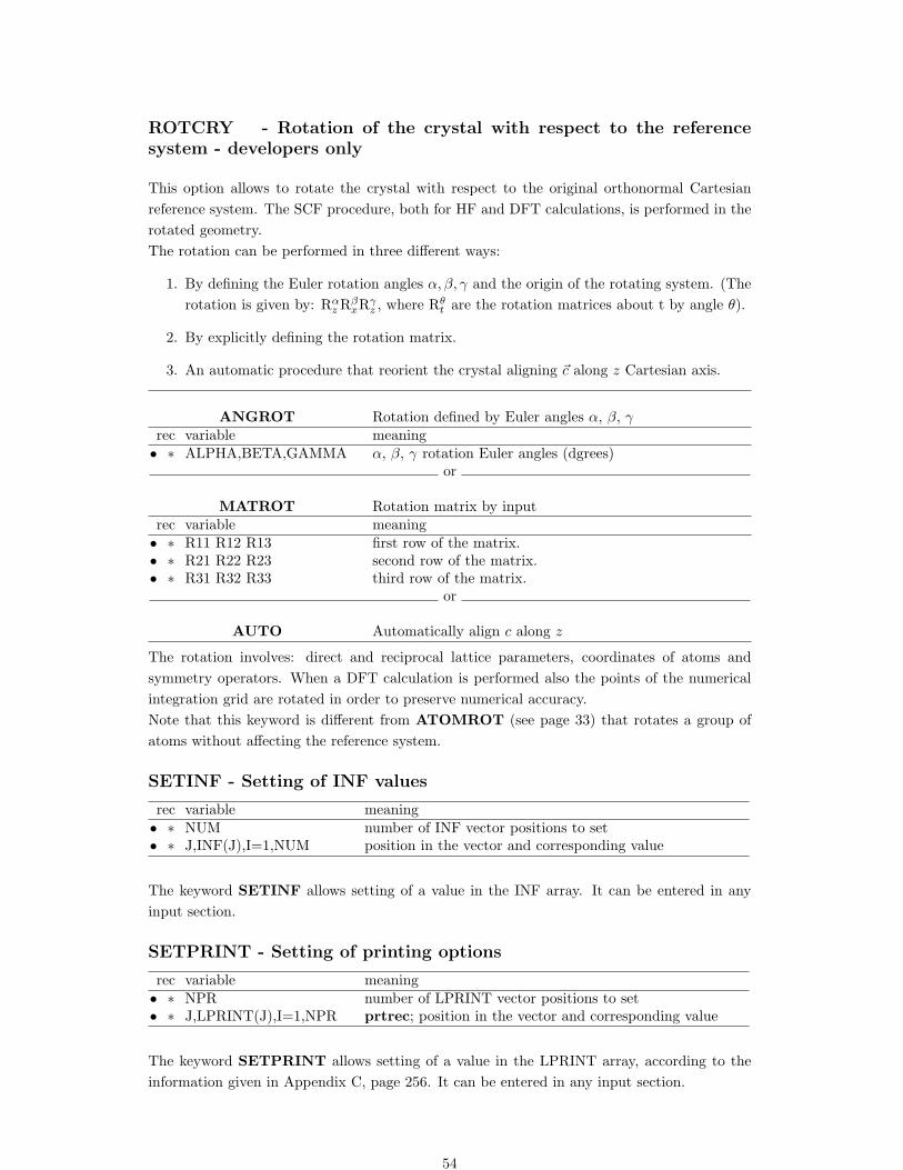
ROTCRY - Rotation of the crystal with respect to the referencesystem - developers only

This option allows to rotate the crystal with respect to the original orthonormal Cartesianreference system. The SCF procedure, both for HF and DFT calculations, is performed in therotated geometry.The rotation can be performed in three different ways:

1. By defining the Euler rotation angles α, β, γ and the origin of the rotating system. (Therotation is given by: Rα

z RβxRγ

z , where Rθt are the rotation matrices about t by angle θ).

2. By explicitly defining the rotation matrix.

3. An automatic procedure that reorient the crystal aligning ~c along z Cartesian axis.

ANGROT Rotation defined by Euler angles α, β, γrec variable meaning• ∗ ALPHA,BETA,GAMMA α, β, γ rotation Euler angles (dgrees)

or

MATROT Rotation matrix by inputrec variable meaning• ∗ R11 R12 R13 first row of the matrix.• ∗ R21 R22 R23 second row of the matrix.• ∗ R31 R32 R33 third row of the matrix.

or

AUTO Automatically align c along z

The rotation involves: direct and reciprocal lattice parameters, coordinates of atoms andsymmetry operators. When a DFT calculation is performed also the points of the numericalintegration grid are rotated in order to preserve numerical accuracy.Note that this keyword is different from ATOMROT (see page 33) that rotates a group ofatoms without affecting the reference system.

SETINF - Setting of INF values

rec variable meaning• ∗ NUM number of INF vector positions to set• ∗ J,INF(J),I=1,NUM position in the vector and corresponding value

The keyword SETINF allows setting of a value in the INF array. It can be entered in anyinput section.

SETPRINT - Setting of printing options

rec variable meaning• ∗ NPR number of LPRINT vector positions to set• ∗ J,LPRINT(J),I=1,NPR prtrec; position in the vector and corresponding value

The keyword SETPRINT allows setting of a value in the LPRINT array, according to theinformation given in Appendix C, page 256. It can be entered in any input section.

54

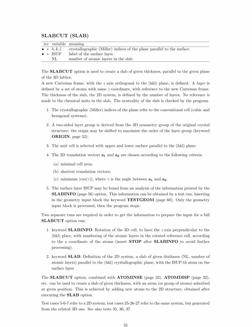
SLABCUT (SLAB)

rec variable meaning• ∗ h, k, l crystallographic (Miller) indices of the plane parallel to the surface• ∗ ISUP label of the surface layer

NL number of atomic layers in the slab

The SLABCUT option is used to create a slab of given thickness, parallel to the given planeof the 3D lattice.A new Cartesian frame, with the z axis orthogonal to the (hkl) plane, is defined. A layer isdefined by a set of atoms with same z coordinate, with reference to the new Cartesian frame.The thickness of the slab, the 2D system, is defined by the number of layers. No reference ismade to the chemical units in the slab. The neutrality of the slab is checked by the program.

1. The crystallographic (Miller) indices of the plane refer to the conventional cell (cubic andhexagonal systems).

2. A two-sided layer group is derived from the 3D symmetry group of the original crystalstructure: the origin may be shifted to maximize the order of the layer group (keywordORIGIN, page 52).

3. The unit cell is selected with upper and lower surface parallel to the (hkl) plane.

4. The 2D translation vectors a1 and a2 are chosen according to the following criteria:

(a) minimal cell area;

(b) shortest translation vectors;

(c) minimum |cos(γ)|, where γ is the angle between a1 and a2.

5. The surface layer ISUP may be found from an analysis of the information printed by theSLABINFO (page 56) option. This information can be obtained by a test run, insertingin the geometry input block the keyword TESTGEOM (page 60). Only the geometryinput block is processed, then the program stops.

Two separate runs are required in order to get the information to prepare the input for a fullSLABCUT option run:

1. keyword SLABINFO: Rotation of the 3D cell, to have the z axis perpendicular to the(hkl) place, with numbering of the atomic layers in the rotated reference cell, accordingto the z coordinate of the atoms (insert STOP after SLABINFO to avoid furtherprocessing).

2. keyword SLAB: Definition of the 2D system, a slab of given thickness (NL, number ofatomic layers) parallel to the (hkl) crystallographic plane, with the ISUP-th atom on thesurface layer

The SLABCUT option, combined with ATOMINSE (page 32), ATOMDISP (page 32),etc. can be used to create a slab of given thickness, with an atom (or group of atoms) adsorbedat given position. This is achieved by adding new atoms to the 2D structure, obtained afterexecuting the SLAB option.

Test cases 5-6-7 refer to a 2D system; test cases 25-26-27 refer to the same system, but generatedfrom the related 3D one. See also tests 35, 36, 37.

55

SLABINFO - 3D cell with z axis orthogonal to a given plane

rec variable meaning• ∗ h,k,l Crystallographic (Miller) indices of the basal layer of the new 3D unit cell

1. A new unit cell is defined, with two lattice vectors perpendicular to the [hkl] direction.The indices refer to the Bravais lattice of the crystal; the hexagonal lattice is used forthe rhombohedral systems, the cubic lattice for cubic systems (non primitive).

2. A new Cartesian reference system is defined, with the xy plane parallel to the (hkl) plane.

3. The atoms in the reference cell are re-ordered according to their z coordinate, in orderto recognize the layered structure, parallel to the (hkl) plane.

4. The layers of atoms are numbered. This information is necessary for generating the inputdata for the SLABCUT option.

5. After neighboring analysis, the program stops. If the keyword ROTATE was entered,execution continues. The shape of the new cell may be very different, computationalparameters must be carefully checked.

6. the keyword ORIGIN can be used to shift the origin after the rotation of the cell, andminimize the number of symmetry operators with translational component. Useful tomaximize the point group of the 2D system that can be generated from 3D using thekeyword SLABCUT (page 55).

STOP

Execution stops immediately. Subsequent input records are not processed.

STRUCPRT

A formatted deck with cell parameters and atoms coordinates (bohr) in cartesian reference iswritten in the file STRUC.INCOOR . See appendix D, page 263.

SUPERCEL

rec variable meaning• ∗ E expansion matrix E (IDIMxIDIM elements, input by rows: 9 reals (3D); 4 reals

(2D); 1 real (1D)

A supercell is obtained by defining the new unit cell vectors as linear combinations of theprimitive cell unit vectors (See SUPERCON for crystallographic cell vectors reference). Thepoint symmetry is defined by the number of symmetry operators in the new cell. It may bereduced, not increased.The new translation vectors b′1,b

′2,b

′3 are defined in terms of the old vectors b1,b2,b3 and of

the matrix E, read in input by rows, as follows:

b′1 = e11 · b1 + e12 · b2 + e13 · b3

b′2 = e21 · b1 + e22 · b2 + e23 · b3

b′3 = e31 · b1 + e32 · b2 + e33 · b3

The symmetry is automatically reduced to the point symmetry operators without translationalcomponents and a further reduction of the symmetry is also possible.

56

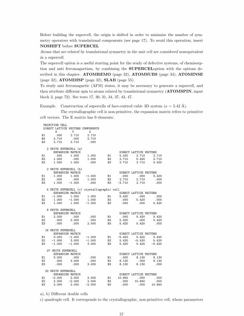
Before building the supercell, the origin is shifted in order to minimize the number of sym-metry operators with translational components (see page 17). To avoid this operation, insertNOSHIFT before SUPERCELAtoms that are related by translational symmetry in the unit cell are considered nonequivalent

in a supercell.The supercell option is a useful starting point for the study of defective systems, of chemisorp-tion and anti ferromagnetism, by combining the SUPERCELoption with the options de-scribed in this chapter: ATOMREMO (page 32), ATOMSUBS (page 34), ATOMINSE(page 32), ATOMDISP (page 32), SLAB (page 55).To study anti ferromagnetic (AFM) states, it may be necessary to generate a supercell, andthen attribute different spin to atoms related by translational symmetry (ATOMSPIN, inputblock 3, page 72). See tests 17, 30, 31, 34, 37, 43, 47.

Example. Construction of supercells of face-centred cubic 3D system (a = 5.42 A).The crystallographic cell is non-primitive, the expansion matrix refers to primitive

cell vectors. The E matrix has 9 elements:

PRIMITIVE CELLDIRECT LATTICE VECTORS COMPONENTS

X Y ZB1 .000 2.710 2.710B2 2.710 .000 2.710B3 2.710 2.710 .000

2 UNITS SUPERCELL (a)EXPANSION MATRIX DIRECT LATTICE VECTORS

E1 .000 1.000 1.000 B1 5.420 2.710 2.710E2 1.000 .000 1.000 B2 2.710 5.420 2.710E3 1.000 1.000 .000 B3 2.710 2.710 5.420

2 UNITS SUPERCELL (b)EXPANSION MATRIX DIRECT LATTICE VECTORS

E1 1.000 1.000 -1.000 B1 .000 .000 5.420E2 .000 .000 1.000 B2 2.710 2.710 .000E3 1.000 -1.000 .000 B3 -2.710 2.710 .000

4 UNITS SUPERCELL (c) crystallographic cellEXPANSION MATRIX DIRECT LATTICE VECTORS

E1 -1.000 1.000 1.000 B1 5.420 .000 .000E2 1.000 -1.000 1.000 B2 .000 5.420 .000E3 1.000 1.000 -1.000 B3 .000 .000 5.420

8 UNITS SUPERCELLEXPANSION MATRIX DIRECT LATTICE VECTORS

E1 2.000 .000 .000 B1 .000 5.420 5.420E2 .000 2.000 .000 B2 5.420 .000 5.420E3 .000 .000 2.000 B3 5.420 5.420 .000


E1 3.000 -1.000 -1.000 B1 -5.420 5.420 5.420E2 -1.000 3.000 -1.000 B2 5.420 -5.420 5.420E3 -1.000 -1.000 3.000 B3 5.420 5.420 -5.420


E1 3.000 .000 .000 B1 .000 8.130 8.130E2 .000 3.000 .000 B2 8.130 .000 8.130E3 .000 .000 3.000 B3 8.130 8.130 .000


E1 -2.000 2.000 2.000 B1 10.840 .000 .000E2 2.000 -2.000 2.000 B2 .000 10.840 .000E3 2.000 2.000 -2.000 B3 .000 .000 10.840

a), b) Different double cellsc) quadruple cell. It corresponds to the crystallographic, non-primitive cell, whose parameters

57

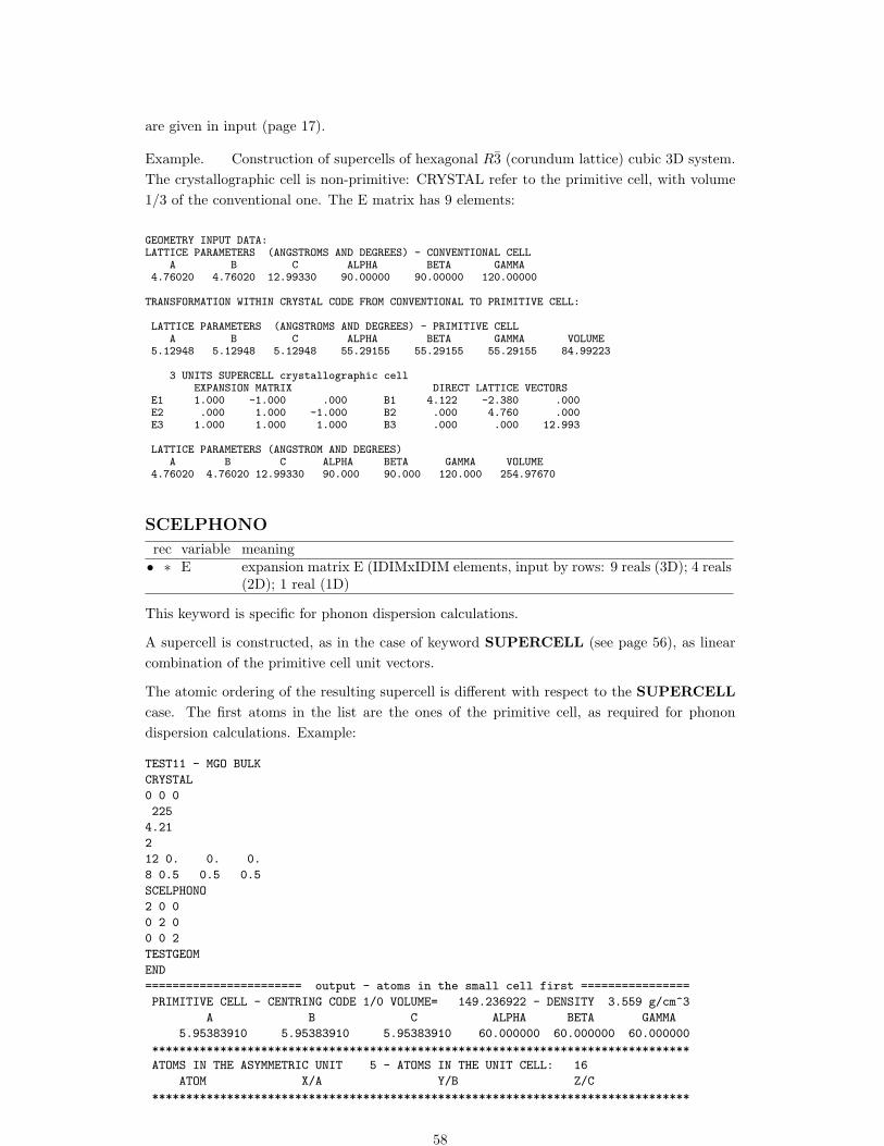
are given in input (page 17).

Example. Construction of supercells of hexagonal R3 (corundum lattice) cubic 3D system.The crystallographic cell is non-primitive: CRYSTAL refer to the primitive cell, with volume1/3 of the conventional one. The E matrix has 9 elements:

GEOMETRY INPUT DATA:LATTICE PARAMETERS (ANGSTROMS AND DEGREES) - CONVENTIONAL CELL

A B C ALPHA BETA GAMMA4.76020 4.76020 12.99330 90.00000 90.00000 120.00000

TRANSFORMATION WITHIN CRYSTAL CODE FROM CONVENTIONAL TO PRIMITIVE CELL:

LATTICE PARAMETERS (ANGSTROMS AND DEGREES) - PRIMITIVE CELLA B C ALPHA BETA GAMMA VOLUME

5.12948 5.12948 5.12948 55.29155 55.29155 55.29155 84.99223

3 UNITS SUPERCELL crystallographic cellEXPANSION MATRIX DIRECT LATTICE VECTORS

E1 1.000 -1.000 .000 B1 4.122 -2.380 .000E2 .000 1.000 -1.000 B2 .000 4.760 .000E3 1.000 1.000 1.000 B3 .000 .000 12.993

LATTICE PARAMETERS (ANGSTROM AND DEGREES)A B C ALPHA BETA GAMMA VOLUME

4.76020 4.76020 12.99330 90.000 90.000 120.000 254.97670

SCELPHONO

rec variable meaning• ∗ E expansion matrix E (IDIMxIDIM elements, input by rows: 9 reals (3D); 4 reals

(2D); 1 real (1D)

This keyword is specific for phonon dispersion calculations.

A supercell is constructed, as in the case of keyword SUPERCELL (see page 56), as linearcombination of the primitive cell unit vectors.

The atomic ordering of the resulting supercell is different with respect to the SUPERCELLcase. The first atoms in the list are the ones of the primitive cell, as required for phonondispersion calculations. Example:

TEST11 - MGO BULK

CRYSTAL

0 0 0

225

4.21

2

12 0. 0. 0.

8 0.5 0.5 0.5

SCELPHONO

2 0 0

0 2 0

0 0 2

TESTGEOM

END

======================= output - atoms in the small cell first ================

PRIMITIVE CELL - CENTRING CODE 1/0 VOLUME= 149.236922 - DENSITY 3.559 g/cm^3

A B C ALPHA BETA GAMMA

5.95383910 5.95383910 5.95383910 60.000000 60.000000 60.000000

*******************************************************************************

ATOMS IN THE ASYMMETRIC UNIT 5 - ATOMS IN THE UNIT CELL: 16

ATOM X/A Y/B Z/C

*******************************************************************************

58

1 T 12 MG 0.000000000000E+00 0.000000000000E+00 0.000000000000E+00

2 T 8 O 2.500000000000E-01 2.500000000000E-01 2.500000000000E-01

3 T 12 MG 0.000000000000E+00 -5.000000000000E-01 0.000000000000E+00

4 F 12 MG 0.000000000000E+00 -5.000000000000E-01 -5.000000000000E-01

5 F 12 MG -5.000000000000E-01 0.000000000000E+00 0.000000000000E+00

6 F 12 MG -5.000000000000E-01 0.000000000000E+00 -5.000000000000E-01

7 F 12 MG -5.000000000000E-01 -5.000000000000E-01 0.000000000000E+00

8 T 12 MG -5.000000000000E-01 -5.000000000000E-01 -5.000000000000E-01

9 F 12 MG 0.000000000000E+00 0.000000000000E+00 -5.000000000000E-01

10 T 8 O 2.500000000000E-01 2.500000000000E-01 -2.500000000000E-01

11 F 8 O 2.500000000000E-01 -2.500000000000E-01 2.500000000000E-01

12 F 8 O 2.500000000000E-01 -2.500000000000E-01 -2.500000000000E-01

13 F 8 O -2.500000000000E-01 2.500000000000E-01 2.500000000000E-01

14 F 8 O -2.500000000000E-01 2.500000000000E-01 -2.500000000000E-01

15 F 8 O -2.500000000000E-01 -2.500000000000E-01 2.500000000000E-01

16 F 8 O -2.500000000000E-01 -2.500000000000E-01 -2.500000000000E-01

TEST11 - MGO BULK

CRYSTAL

0 0 0

225

4.21

2

12 0. 0. 0.

8 0.5 0.5 0.5

SUPERCEL

2 0 0

0 2 0

0 0 2

TESTGEOM

======================= output - atoms of same type first ================

PRIMITIVE CELL - CENTRING CODE 1/0 VOLUME= 149.236922 - DENSITY 3.559 g/cm^3

A B C ALPHA BETA GAMMA

5.95383910 5.95383910 5.95383910 60.000000 60.000000 60.000000

*******************************************************************************

ATOMS IN THE ASYMMETRIC UNIT 5 - ATOMS IN THE UNIT CELL: 16

ATOM X/A Y/B Z/C

*******************************************************************************

1 T 12 MG 0.000000000000E+00 0.000000000000E+00 0.000000000000E+00

2 T 12 MG 0.000000000000E+00 0.000000000000E+00 -5.000000000000E-01

3 F 12 MG 0.000000000000E+00 -5.000000000000E-01 0.000000000000E+00

4 F 12 MG 0.000000000000E+00 -5.000000000000E-01 -5.000000000000E-01

5 F 12 MG -5.000000000000E-01 0.000000000000E+00 0.000000000000E+00

6 F 12 MG -5.000000000000E-01 0.000000000000E+00 -5.000000000000E-01

7 F 12 MG -5.000000000000E-01 -5.000000000000E-01 0.000000000000E+00

8 T 12 MG -5.000000000000E-01 -5.000000000000E-01 -5.000000000000E-01

9 T 8 O -2.500000000000E-01 -2.500000000000E-01 2.500000000000E-01

10 T 8 O -2.500000000000E-01 -2.500000000000E-01 -2.500000000000E-01

11 F 8 O -2.500000000000E-01 2.500000000000E-01 2.500000000000E-01

12 F 8 O -2.500000000000E-01 2.500000000000E-01 -2.500000000000E-01

13 F 8 O 2.500000000000E-01 -2.500000000000E-01 2.500000000000E-01

14 F 8 O 2.500000000000E-01 -2.500000000000E-01 -2.500000000000E-01

15 F 8 O 2.500000000000E-01 2.500000000000E-01 2.500000000000E-01

16 F 8 O 2.500000000000E-01 2.500000000000E-01 -2.500000000000E-01

It can be used to generate a supercell for DISPERSION calculation only.

59

SUPERCON

The first step in geometry definition in CRYSTAL is the transformation of the cell from crystal-lographic to primitive, according to the transformation matrices given in appendix A.5, whenthe crystallographic cell is non-primitive.From the point of view of CRYSTAL, the crystallographic cell is a supercell, in that case.Using the keyword SUPERCON, the crystallographic cell is built from the primitive one,before applying the expansion matrix.See SUPERCEL, page 56 for expansion matrix input instructions.

Note - The easiest way to work on crystallographic cell is the following input:

SUPERCON1. 0. 0.0. 1. 0.0. 0. 1.\

The expansion matrix is the identity, leaving the crystallographic cell unmodified.

SYMMDIR

The symmetry allowed directions, corresponding to internal degrees of freedom are printed.No input data are required.

SYMMOPS

Point symmetry operator matrices are printed in the Cartesian representation. No input dataare required.

SYMMREMO

All the point group symmetry operators are removed. Only the identity operator is left. Thewave function can be computed. No input data are required.Warning: the CPU time may increase by a factor MVF (order of point-group), both in theintegral calculation and in the scf step. The size of the bielectronic integral file may increaseby a factor MVF2.

TENSOR

rec variable meaning• ∗ IORD order of the tensor (≤ 4)

This option evaluates and prints the non zero elements of the tensor of physical properties upto order 4.

TESTGEOM

Execution stops after reading the geometry input block and printing the coordinates of theatoms in the conventional cell. Neighbours analysis, as requested by the keyword NEIGH-BOR, is not executed. The geometry input block must end with the keyword END or ENDG.No other input blocks (basis set etc) are required.

TRASREMO

Point symmetry operators with fractional translation components are removed. It is suggestedto previously add the keyword ORIGIN (page 52), in order to minimize the number of sym-metry operators with finite translation component. No input data are required.

60

USESAED

rec variable meaning• ∗ δ(i),i=1,nsaed δ for each distortion

Given the symmetry allowed elastic distortion (SAED), (printed by the keyword MAKE-SAED, page 45) δ for the allowed distortion are given in input.

61

2.2 Basis set input

Symmetry control

ATOMSYMM printing of point symmetry at the atomic positions 34 –

Basis set modification

CHEMOD modification of the electronic configuration 62 IGHOSTS eliminates nuclei and electrons, leaving BS 64 I


CHARGED allows non-neutral cell 62 –NOPRINT printing of basis set removed 64 –PARAMPRT printing of parameters controlling code dimensions 52 –PRINTOUT setting of printing options 53 ISETINF setting of inf array options 54 ISETPRINT setting of printing options 54 ISTOP execution stops immediately 56 –SYMMOPS printing of point symmetry operators 60 –END/ENDB terminate processing of basis set definition keywords –


GAUSS98 printing of an input file for the GAUSS94/98 package 64 –

Basis set input optional keywords

ATOMSYMM

See input block 1, page 34

CHARGED - charged reference cell

The unit cell of a periodic system must be neutral. This option forces the overall system tobe neutral even when the number of electrons in the reference cell is different from the sumof nuclear charges, by adding a uniform background charge density to neutralize the charge inthe reference cell.

Warning - Do not use for total energy comparison.

CHEMOD - modification of electronic configuration

rec variable meaning• ∗ NC number of configurations to modify• ∗ LA label of the atom with new configuration∗ CH(L),L=1,NS shell charges of the LA-th atom. The number NS of shells must coincide

with that defined in the basis set input.

The CHEMOD keyword allows modifications of the shell charges given in the basis set input,which are used in the atomic wave function routines. The original geometric symmetry ischecked, taking the new electronic configuration of the atoms into account. If the number ofsymmetry operators should be reduced, information on the new symmetry is printed, and theprogram stops. No automatic reduction of the symmetry is allowed. Using the informationprinted, the symmetry must be reduced by the keyword MODISYMM (input block 1, page45).

62

See test 37. MgO supercell, with a Li defect. The electronic configuration of the oxygen nearestto Li corresponds to O−, while the electronic configuration of those in bulk MgO is O2−. Thebasis set of oxygen is unique, while the contribution of the two types of oxygen to the initialdensity matrix is different.

END

Terminate processing of block 2, basis set, input. Execution continues. Subsequent inputrecords are processed, if required.

GAUSS98 - Printing of input file for GAUSS98 package

The keyword GAUSS98 writes in file GAUSSIAN.DAT an input deck to run Gaussian (Gaus-sian 98 or Gaussian03) [52, 51]. The deck can be prepared without the calculation of the wavefunction by entering the keyword TESTPDIM in input block 3 (page 101). For periodicsystems, coordinates and basis set for all the atoms in the reference cell only are written (noinformation on translational symmetry).If the keyword is entered many times, the data are overwritten. The file GAUSSIAN.DATcontains the data corresponding to the last call.The utility program gautocry reads basis set input in Gaussian format (as prepared byhttp://www.emsl.pnl.gov/forms/basisform.html) and writes it in CRYSTAL format. Noinput data required.

1. The route card specifies:

method HFbasis set GEN 5D 7Ftype of job SPgeometry UNITS=AU GEOM=COORD

2. The title card is the same as in CRYSTAL input.

3. The molecule specification defines the molecular charge as the net charge in the referencecell. If the system is not closed shell, the spin multiplicity is indicated with a string ”??”,and must be defined by the user.

4. Input for effective core pseudopotentials is not written. In the route card PSEUDO =

CARDS is specified; the pseudopotential parameters used for the crystal calculation areprinted in the crystal output.

5. The scale factors of the exponents are all set to 1., as the exponents are already scaled.

6. the input must be edited when different basis sets are used for atoms with the sameatomic number (e.g., CO on MgO, when the Oxygen basis set is different in CO and inMgO)

Warning: Only for 0D systems! The programs does not stop when the keyword GAUSS98is entered for 1-2-3D systems. Coordinates and basis set of all the atoms in the primitive cellare written, formatted, in file GAUSSIAN.DAT, following Gaussian scheme.

Warning If you run Gaussian 98 using the input generated by CRYSTAL with the keywordGAUSS98, you do not obtain the same energy. There are 3 main differences between a standardCRYSTAL run and a GAUSSIAN run.

1. CRYSTAL adopts by default bipolar expansion to compute coulomb integrals when thetwo distributions do not overlap. To compute all 2 electron integrals exactly, insertkeyword NOBIPOLA in input block 3;

2. CRYSTAL adopts truncation criteria for Coulomb and exchange sums: to remove them,in input block 3 insert:

63

TOLINTEG20 20 20 20 20

3. CRYSTAL adopts the NIST conversion factor bohr/Angstrom CODATA98:1 A= 0.5291772083 bohrTo modify the value, in input block 1 insert:

BOHRANGSvalue_of_new_conversion_factor

GHOSTS

rec variable meaning• ∗ NA number of atoms to be transformed into ghosts• ∗ LA(L),L=1,NA label of the atoms to be transformed.

Selected atoms may be transformed into ghosts, by deleting the nuclear charge and the shellelectron charges, but leaving the basis set centred at the atomic position. The conventionalatomic number is set to zero., the symbol is “XX”.If the system is forced to maintain the original symmetry (KEEPSYMM), all the atomssymmetry related to the given one are transformed into ghosts.Useful to create a vacancy (Test 37), leaving the variational freedom to the defective regionand to evaluate the basis set superposition error (BSSE), in a periodic system. The periodicstructure is maintained, and the energy of the isolated components computed, leaving the basisset of the other one(s) unaltered. For instance, the energy of a mono-layer of CO molecules ontop of a MgO surface can be evaluated including the basis functions of the first layer of MgO,or, vice-versa, the energy of the MgO slab including the CO ad-layer basis functions.See test36 and test37.

Warning Do not use with ECP.

Warning The keyword ATOMREMO (input block 1, page 32) creates a vacancy, removingnuclear charge, electron charge, and basis functions. The keyword GHOSTS creates a vacancy,but leaves the basis functions at the site, so allowing better description of the electron densityin the vacancy.Warning - Removal of nuclear and electron charge of the atoms selected is done after completeprocessing of the input. They look still as ”atoms” in the printed output before that operation.

NOPRINT

Printing of basis set is removed. No input data required.

PARAMPRT - Printing of parametrized dimensions

See input block 1, page 52.







64

STOP


TEST[BS]

Basis set input is checked, then execution stops. Subsequent input records (block3) are notprocessed.

SYMMOPS


Effective core pseudo-potentials - ECP

rec variable value meaning• A PSN pseudo-potential keyword:

HAYWLC Hay and Wadt large core ECP.HAYWSC Hay and Wadt small core ECP.BARTHE Durand and Barthelat ECP.DURAND Durand and Barthelat ECP.INPUT free ECP - input follows.

if PSN = INPUT insert II• ∗ ZNUC effective core charge (ZN in eq. 2.16).

M Number of terms in eq. 2.17M0 Number of terms in eq. 2.18 for ` =0.M1 Number of terms in eq. 2.18 for ` =1.M2 Number of terms in eq. 2.18 for ` =2.M3 Number of terms in eq. 2.18 for ` =3.M4 Number of terms in eq. 2.18 for ` =4. - CRYSTAL09

insert M+M0+M1+M2+M3+M4 records II• ∗ ALFKL Exponents of the Gaussians: αk`.

CGKL Coefficient of the Gaussians: Ck`.NKL Exponent of the r factors: nk`.

Valence-electron only calculations can be performed with the aid of effective core pseudo-potentials (ECP). The ECP input must be inserted into the basis set input of the atoms withconventional atomic number > 200.

The form of pseudo-potential Wps implemented in CRYSTAL is a sum of three terms: aCoulomb term (C), a local term (W0) and a semi-local term (SL):

Wps = C +W0 + SL (2.15)

where:C = −ZN/r (2.16)

W0 =M∑

k=1

rnkCke−αkr2

(2.17)

SL =4∑

`=0

[M∑k=1

rnk`Ck`e−αk`r2

]P` (2.18)

ZN is the effective nuclear charge, equal to total nuclear charge minus the number of electronsrepresented by the ECP, P` is the projection operator related to the ` angular quantum number,and M, nk, αk, M`, nk`, Ck`, αk` are atomic pseudo-potential parameters.

65

1. Hay and Wadt (HW) ECP ([69, 67]) are of the general form 2.15. In this case, the NKLvalue given in the tables of ref. [69, 67] must be decreased by 2 (2 → 0, 1 → -1, 0 → -2).

2. Durand and Barthelat (DB) ([8] - [45], [9], [10]), and Stuttgart-Dresden [63] ECPs containonly the Coulomb term C and the semi-local SL term.

3. In Durand and Barthelat ECP the exponential coefficient α in SL depends only on ` (i.e.it is the same for all the Mk terms).

SL =3∑

`=0

e−α`r2[M∑k=1

rnk`Ck`]P` (2.19)

The core orbitals replaced by Hay and Wadt large core and Durand-Barthelat ECPs are asfollows:

Li-Ne = [He]Na-Ar = [Ne]first series = [Ar]second series = [Kr]third series = [Xe]4f14.

The core orbitals replaced by Hay and Wadt small core ECPs are as follows:

K-Cu = [Ne]Rb-Ag = [Ar] 3d10

Cs-Au = [Kr] 4d10 .

The program evaluates only those integrals for which the overlap between the charge distri-bution ϕ0

µ ϕgν (page 221) and the most diffuse Gaussian defining the pseudopotential is larger

than a given threshold Tps (the default value is 10−5). See also TOLPSEUD (Section 1.3).

Pseudopotential libraries

The following periodic tables show the effective core pseudo-potentials included as internaldata in the CRYSTAL code.

66

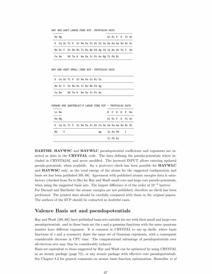
HAY AND WADT LARGE CORE ECP. CRYSTAL92 DATA

------- ------------------


------------------------------------------------------


------------------------------------------------------

Rb Sr Y Zr Nb Mo Tc Ru Rh Pd Ag Cd In Sn Sb Te I Xe

------------------------------------------------------

Cs Ba Hf Ta W Re Os Ir Pt Au Hg Tl Pb Bi

------------------------------------------------------

HAY AND WADT SMALL CORE ECP. CRYSTAL92 DATA

-------------------------------------------------------

K Ca Sc Ti V Cr Mn Fe Co Ni Cu

-------------------------------------------------------

Rb Sr Y Zr Nb Mo Tc Ru Rh Pd Ag

-------------------------------------------------------

Cs Ba Hf Ta W Re Os Ir Pt Au

-------------------------------------------------------

DURAND AND BARTHELAT’S LARGE CORE ECP - CRYSTAL92 DATA

------ ------------------

Li Be B C N O F Ne

------ ------------------


-------------------------------------------------------


-------------------------------------------------------

Rb Y Ag In Sn Sb I

-------------------------------------------------------

Tl Pb Bi

-------------------------------------------------------

BARTHE, HAYWSC and HAYWLC pseudopotential coefficients and exponents are in-serted as data in the CRYSTAL code. The data defining the pseudo-potentials where in-cluded in CRYSTAL92, and never modified. The keyword INPUT allows entering updatedpseudo-potentials, when available. An a posteriori check has been possible for HAYWLCand HAYWSC only, as the total energy of the atoms for the suggested configuration andbasis set has been published [69, 68]. Agreement with published atomic energies data is satis-factory (checked from Na to Ba) for Hay and Wadt small core and large core pseudo-potentials,when using the suggested basis sets. The largest difference is of the order of 10−3 hartree.For Durand and Barthelat the atomic energies are not published, therefore no check has beenperformed. The printed data should be carefully compared with those in the original papers.The authors of the ECP should be contacted in doubtful cases.

Valence Basis set and pseudopotentials

Hay and Wadt ([69, 68]) have published basis sets suitable for use with their small and large corepseudopotentials. and in those basis set the s and p gaussian functions with the same quantumnumber have different exponent. It is common in CRYSTAL to use sp shells, where basisfunctions of s and p symmetry share the same set of Gaussian exponents, with a consequentconsiderable decrease in CPU time. The computational advantage of pseudopotentials overall-electron sets may thus be considerably reduced.Basis set equivalent to those suggested by Hay and Wadt can be optimized by using CRYSTAL

as an atomic package (page 72), or any atomic package with effective core pseudopotentials.See Chapter 8.2 for general comments on atomic basis function optimization. Bouteiller et al

67

[16] have published a series of basis sets optimized for Durand and Barthelat ECPs.

Stuttgart-Dresden ECP (formerly STOLL and PREUSS ECP)

The most recent pseudopotential parameters, optimized basis sets, a list of references andguidelines for the choice of the pseudopotentials can be found in:http://www.theochem.uni-stuttgart.de/pseudopotentials/index.en.html

The clickable periodic table supplies, in CRYSTAL format, ECP to be used in CRYSTAL viathe INPUT keyword (basis set input, block2, page 65).http://www.theochem.uni-stuttgart.de/pseudopotentials/clickpse.en.html

RCEP Stevens et al.

Conversion of Stevens et al. pseudopotentials An other important family of pseudopotentialsfor the first-, second-, third-, fourth and fifth-row atoms of the periodic Table (excludingthe lanthanide series) is given by Stevens et al. [121, 122]. Analytic Relativistic CompactEffective Potential (RCEP) are generated in order to reproduce the ”exact” pseudo-orbitalsand eigenvalues as closely as possible. The analytic RCEP expansions are given by:

r2Vl(r) =∑

k

Alkrnl,ke−Blkr2

An example of data for Ga atom (Table 1, page 616 of the second paper) is:

Alk nlk Blk

Vd -3.87363 1 26.74302Vs−d 4.12472 0 3.46530

260.73263 2 9.11130-223.96003 2 7.89329

Vp−d 4.20033 0 79.99353127.99139 2 17.39114

The corresponding Input file for the CRYSTAL program will be as follows:

INPUT21. 1 3 2 0 0

26.74302 -3.87363 -13.46530 4.12472 -29.11130 260.73263 07.89329 -223.96003 0

79.99353 4.20033 -217.39114 127.99139 0

Note that for the r-exponent (nlk), -2 has been subtracted to the value given in their papers,as in the case of Hay and Wadt pseudopotentials.

68

2.3 Computational parameters, hamiltonian,SCF control

Single particle Hamiltonian

RHF Restricted Closed Shell 96 –UHF Unrestricted Open Shell 102 –DFT DFT Hamiltonian 102 –

SPIN spin-polarized solution 75 –Choice of the exchange-correlation functionalsCORRELAT correlation functional 74 I

LYP Lee-Yang-Parr [78] (GGA)P86 Perdew 86 [88] (LDA)PBE Perdew-Becke-Ernzerhof [90] (GGA)PBESOL GGA. PBE functional revised for solids [96]PWGGA Perdew-Wang 91 (GGA)PWLSD Perdew-Wang 92 [92, 93, 91] (GGA)PZ Perdew-Zunger [94] (LDA)VBH von Barth-Hedin [127] (LDA)WL GGA - Wilson-Levy [133]VWN Vosko,-Wilk-Nusair [128] (LDA)

EXCHANGE exchange functional 75 IBECKE Becke [13] (GGA)LDA Dirac-Slater [34] (LDA)PBE Perdew-Becke-Ernzerhof [90] (GGA)PBESOL GGA. PBE functional revised for solids [96]PWGGA Perdew-Wang 91 (GGA)SOGGA second order GGA. [136]VBH von Barth-Hedin [127] (LDA)WCGGA GGA - Wu-Cohen [135]

Global keywords: exchange+correlationB3PW B3PW parameterization 76 –B3LYP B3LYP parameterization 76 –PBE0 Adamo and Barone [2] 76SOGGAXC see [136] 76Custom made dft exchange-local exchangeHYBRID hybrid mixing 76 INONLOCAL local term parameterization 76 I

69

Numerical accuracy controlANGULAR definition of angular grid IBATCHPNT grid point grouping for integration I[BECKE] selection of Becke weights (default) –[CHUNKS] max n. points in a batch for numerical int. ILGRID ”large” predefined grid IRADSAFE safety radius for grid point screening IRADIAL definition of radial grid ISAVIN selection of Savin weights –TOLLDENS density contribution screening 6 ITOLLGRID grid points screening 14 IXLGRID ”extra large” predefined grid IXXLGRID ”extra extra large” predefined grid IAtomic parameters controlRADIUS customized atomic radius 81 IFCHARGE customized formal atomic charge 81 IAuxiliaryPRINT extended printingEND close DFT input block

Numerical accuracy and computational parameters control

BIPOLAR Bipolar expansion of bielectronic integrals 73 IBIPOSIZE size of coulomb bipolar expansion buffer 73 IEXCHSIZE size of exchange bipolar expansion buffer 73 IINTGPACK Choice of integrals package 0 92 INOBIPCOU Coulomb bielectronic integrals computed exactly 95 –NOBIPEXCH Exchange bielectronic integrals computed exactly 95 –NOBIPOLA All bielectronic integrals computed exactly 95 –POLEORDR Maximum order of multipolar expansion 4 96 ITOLINTEG Truncation criteria for bielectronic integrals 6 6 6 6 12 102 ITOLPSEUD Pseudopotential tolerance 6 102 I

Type of executionMPP MPP execution 93

Type of run

ATOMHF Atomic wave functions 72 ISCFDIR SCF direct (mono+biel int computed) 96 –EIGS S(k) eigenvalues - basis set linear dependence check 81 –FIXINDEX Reference geometry to classify integrals 86 –

Basis set - AO occupancy

FDAOSYM f and d degeneracies analysis 83 IFDAOCCUP f and d orbital occupation guess 84 IGUESDUAL Density matrix guess - different Basis set 89 I

Integral file distribution

BIESPLIT writing of bielectronic integrals in n files n = 1 ,max=10 73 IMONSPLIT writing of mono-electronic integrals in n file n = 1 , max=10 93 I

Numerical accuracy control and convergence tools

70

ANDERSON Fock matrix mixing 71 IBROYDEN Fock matrix mixing 73 IFMIXING Fock/KS matrix (cycle i and i-1) mixing 0 87 ILEVSHIFT level shifter no 92 IMAXCYCLE maximum number of cycles 50 93 ISMEAR Finite temperature smearing of the Fermi surface no 99 ITOLDEE convergence on total energy 5 102 ITOLDEP convergence on density matrix 16 102 I

Initial guess

EIGSHIFT alteration of orbital occupation before SCF no 82 IEIGSHROT rotation of the reference frame no 82 IGUESSP density matrix from a previous run 91 –GUESSPAT superposition of atomic densities 91 –


ATOMSPIN setting of atomic spin to compute atomic densities 72 IBETALOCK beta electrons locking 73 ISPINLOCK spin difference locking 101 ISPINEDIT editing of the spin density matrix used as SCF guess 100 I


END terminate processing of block3 input –KSYMMPRT printing of Bloch functions symmetry analysis 92 –NEIGHBOR number of neighbours to analyse in PPAN 51 IPARAMPRT output of parameters controlling code dimensions 52 –PRINTOUT setting of printing options 53 INOSYMADA No Symmetry Adapted Bloch Functions 95 –SYMADAPT Symmetry Adapted Bloch Functions (default) 101 –SETINF setting of inf array options 54 ISETPRINT setting of printing options 54 ISTOP execution stops immediately 56 –TESTPDIM stop after symmetry analysis 101 –TEST[RUN] stop after integrals classification and disk storage estimate 101 –


NOFMWF wave function formatted output not written in file fort.98. 95 –SAVEWF wave function data written every two SCF cycles 97 –

Post SCF calculations

POSTSCF post-scf calculations when convergence criteria not satisfied 96 –EXCHGENE exchange energy evaluation (spin polarized only) 83 –GRADCAL analytical gradient of the energy 87 –PPAN population analysis at the end of the SCF no 96

Computational parameters, hamiltonian, SCF controloptional keywords

ANDERSON

Anderson’s method [3], as proposed by Hamann [65], is applied. No input data are required.

71

See test49 dft, a metallic Lithium 5 layers slab, PWGGA Hamiltonian.

ATOMHF - Atomic wave function calculation

The Hartree-Fock atomic wave functions for the symmetry unique atoms in the cell are com-puted by the atomic program [6]. Full input (geometry, basis set, general information, SCF) isprocessed. No input data are required. The density matrix, constructed from a superpositionof atomic densities, is computed and written on Fortran unit 9, along with the wave functioninformation. The crystal program then stops. It is then possible to compute charge density(ECHG) and classical electrostatic potential (CLAS) maps by running the program proper-

ties. This option is an alternative to the keyword PATO in the program properties (page180), when the calculation of the periodic wave function is not required. The atomic wavefunction, eigenvalues and eigenvectors, can be printed by setting the printing option 71.

1. The atomic basis set may include diffuse functions, as no periodic calculation is carriedout.

2. A maximum of two open shells of different symmetry (s, p, d) are allowed in the electronicconfiguration. In the electronic configuration given in input the occupation number ofthe shells must follow the rules given in Section 1.2.

3. For each electronic configuration, the highest multiplicity state is computed. Multiplicitycannot be chosen by the user.

Warning: DFT wave function for isolated atoms can not be computed.

ATOMSPIN - Setting of atomic spin

rec variable meaning• ∗ NA number of atoms to attribute a spin• ∗ LA,LS(LA),L=1,NA atom labels and spin (1, 0, -1)

The setting of the atomic spins is used to compute the density matrix as superposition ofatomic densities (GUESSPAT must be SCF initial guess); it does not work with GUESSP).The symmetry of the lattice may be reduced by attributing a different spin to geometricallysymmetry related atoms. In such cases a previous symmetry reduction should be performedusing the MODISYMM keyword. The program checks the symmetry taking the spin of theatoms into account. If the spin pattern does not correspond to the symmetry, the programprints information on the new symmetry, and then stops.The formal spin values are given as follows:

1 atom spin is taken to be alpha;0 atom spin is irrelevant;-1 atom spin is taken to be beta.

In a NiO double-cell (four atoms, Ni1 Ni2 O1 O2) we might use:

atom Ni1 Ni2

spin 1 1 for starting ferromagnetic solutions: ↑ ↑spin 1 -1 for starting anti ferromagnetic solutions: ↑ ↓

SPINLOCK forces a given nα − nβ electrons value: to obtain a correct atomic spin densityto start SCF process, the atomic spins must be set even for the ferromagnetic solution.See test 30 and 31.

72

BETALOCK - Spin-polarized solutions

rec variable meaning• ∗ INF97 nβ electrons∗ INF98 number of cycles the nβ electrons is maintained

The total number of of β electrons at all k points can be locked at the input value. The numberof α electrons is locked to (N + INF95)/2, where N is the total number of electrons in theunit cell. INF95 must be odd when the number of electrons is odd, even when the number ofelectrons is even. See SPINLOCK for alternative way to define spin setting.

BIESPLIT - Splitting of large bielectronic integral files

rec variable meaning• ∗ NFILE number of files to be used 1 (max 10)

Very compact crystalline systems, and/or very diffuse basis functions and/or very tight toler-ances can produce billions integrals to be stored. The storage of bielectronic integrals can beavoided by running the direct SCF code scfdir rather than the standard SCF, at the expensesof a certain amount of CPU time.When the standard SCF code is used, distributing the integrals on several disk files can improveperformance.

BIPOLAR - Bipolar expansion approximation control

rec variable meaning• ∗ ITCOUL overlap threshold for Coulomb 14∗ ITEXCH overlap threshold for exchange 10

The bipolar approximation is applied in the evaluation of the Coulomb and exchange integrals(page 225). ITCOUL and ITEXCH can be assigned any intermediate value between the defaultvalues (14 and 10) (see page 225) and the values switching off the bipolar expansion (20000and 20000).

BIPOSIZE -Size of buffer for Coulomb integrals bipolar expansion

rec variable meaning• ∗ ISIZE size of the buffer in words

Size (words) of the buffer for bipolar expansion of Coulomb integrals (default value 100000.The size of the buffer is printed in the message:

BIPO BUFFER LENGTH (WORDS) = XXXXXXX

or

COULOMB BIPO BUFFER TOO SMALL - TO AVOID I/O SET BIPOSIZE = XXXXXX

BROYDEN

rec variable meaning• ∗ W0 W0 parameter in Anderson’s paper [75]∗ IMIX percent of Fock/KS matrices mixing when Broyden method is switched on∗ ISTART SCf iteration after which Broyden method is active (minimum 2)

73

A modified Broyden [18] scheme, following the method proposed by Johnson [75], is appliedafter the ISTART SCF iteration, with IMIX percent of Fock/KS matrices simple mixing. Thevalue of % mixing given in input after the keyword FMIXING is overridden by the new one.Level shifter should be avoided when Broyden method is applied.Suggested values:

FMIXING

80

BROYDEN

0.0001 50 2

See test50 dft, a metallic Lithium 5 layers slab, PWGGA Hamiltonian.

END

Terminate processing of block 3,(last input block). Execution continues. Subsequent inputrecords are not processed.

DFT

The Kohn-Sham [76, 74] DFT code is controlled by keywords, that must follow the generalkeyword DFT, in any order. These keywords can be classified into four groups:

1 Choice of the exchange-correlation functionals

2 Integration grid and numerical accuracy control (optional)

3 DF energy gradient (optional)

4 Atomic parameters (optional)

The DFT input block ends with the keyword END or ENDDFT. Default values are sup-plied for all computational parameters. Choice of exchange and/or correlation potential ismandatory.

1. Choice of the exchange-correlation functionals

EXCHANGE and CORRELAT keywords, each followed by an alpha-numeric record, allowthe selection of the exchange and correlation functionals.If the correlation potential is not set (keyword CORRELAT), an exchange-only potential isused in the Hamiltonian. If the exchange potential is not set (keyword EXCHANGE), theHartree-Fock potential is used.

74

CORRELAT Correlation Potential (default: no correlation).Insert one of the following keywords II

LYP GGA. Lee-Yang-Parr [78]P86 GGA. Perdew 86 [88]PBE GGA. Perdew-Burke-Ernzerhof [90]PBESOL GGA. PBE functional revised for solids [96]PWLSD LSD. Perdew-Wang parameterization of the Ceperley-Alder free electron

gas correlation results [91]PWGGA GGA. Perdew-Wang [95]PZ LSD. Perdew-Zunger parameterization of the Ceperley-Alder free electron

gas correlation results [94]VBH LSD. von Barth-Hedin [127]WL GGA - Wilson-Levy [133]VWN LSD. Vosko-Wilk-Nusair parameterization of the Ceperley-Alder free elec-

tron gas correlation results [128]

EXCHANGE Exchange potential (default: Hartree-Fock exchange).Insert one of the following keywords II

BECKE GGA. Becke [13]LDA LSD. Dirac-Slater [34]PBE GGA. Perdew-Becke-Ernzerhof [90]PBESOL GGA. PBE functional revised for solids [96]PWGGA GGA. Perdew-Wang [95]SOGGA second order GGA. [136]VBH LSD. von Barth-Hedin [127]WCGGA GGA - Wu-Cohen [135]

All functionals are formulated in terms of total density and spin density. Default is totaldensity. To use functionals of spin density insert the keyword SPIN.

SPIN unrestricted spin DF calculation (default: restricted)

It is also possible to incorporate part of the exact Hartree-Fock exchange into the exchangefunctional through the keyword HYBRID. Any mixing (0-100) of exact Hartree-Fock andDFT exchange can be used.NONLOCAL allows modifying the relative weight of the local and non-local part both inthe exchange and the correlation potential with respect to standard definition of GGA typepotentials.

75

HYBRID Hybrid method - 1 record follows:• ∗A Fock exchange percentage (default 100.)

NONLOCAL setting of non-local weighting parameters - 1 record follows:• ∗B exchange weight of the non-local part of exchange

C weight of the non-local correlation

B3PW Becke’s 3 parameter functional [14] combined with the non-local correla-tion PWGGA [89, 92, 93, 91]

B3LYP Becke’s 3 parameter functional [14] combined with the non-local correla-tion LYP

PBE0 Adamo and Barone [2]

SOGGAXC see [136]

B3PW, B3LYP, PBE0 and SOGGAXC are global keywords, defining hybrid exchange-correlation functionals completely. They replace the following sequences:

B3PWcorresponds to the sequence:EXCHANGEBECKECORRELATPWGGAHYBRID20NONLOCAL0.9 0.81

B3LYPcorresponds to the sequence:EXCHANGEBECKECORRELATLYPHYBRID20NONLOCAL0.9 0.81

PBE0corresponds to the sequence:EXCHANGEPBECORRELATPBEHYBRID25

SOGGAXCcorresponds to the sequence:EXCHANGESOGGACORRELATPBE

B3LYP in CRYSTAL is based on the ’exact’ form of the Vosko-Wilk-Nusair correlation poten-tial (corresponds to a fit to the Ceperley-Alder data). In the original paper [128]) it is reportedas functional V, which is used to extract the ’local’ part of the LYP correlation potential.The Becke’s 3 parameter functional can be written as:

Exc = (1−A) ∗ (ELDAx +B ∗ EBECKE

x ) +A ∗ EHFx + (1− C) ∗ EV WN

c + C ∗ ELY Pc

A, B, and C are the input data of HYBRYD and NONLOCAL.

Examples of possible selection of the correlation and exchange functionals are:

76

exchange correlation—– PWGGA Hartree-Fock exchange, non local Perdew-Wang correlation.LDA VWN probably the most popular LDA formulationVBH VBH was the most popular LDA scheme in the early LDA solid state

applications (1975-1985).PWGGA PWGGA - - - - - -BECKE LYP - - - - - -

2. Integration grid and numerical accuracy control

No input data are required: Becke weights are chosen by default, as well as a set of safe valuesfor the computational parameters of integration.The generation of grid points in CRYSTAL is based on an atomic partition method, originallydeveloped by Becke [11] for molecular systems and then extended to periodic systems [124].Each atomic grid consists of a radial and an angular distribution of points. Grid points aregenerated through a radial and an angular formula: Gauss-Legendre radial quadrature andLebedev two-dimensional angular point distribution are used.Lebedev angular grids are classified according to progressive accuracy levels, as given in thefollowing table:

LEV CR98 ` Nang LEV CR98 ` Nang

1 1 9 38 16 53 9742 2 11 50 17 59 12023 13 74 * 18 65 14544 15 86 19 71 17305 3 17 110 20 77 20306 19 146 21 83 23547 21 170 22 89 27028 4 23 194 23 95 30749 25 230 * 24 101 347010 5 27 266 * 25 107 38911 6 29 302 26 113 433412 31 350 27 119 480213 7 35 434 28 125 529414 41 590 29 131 581015 47 770

Index of Lebedev accuracy levelsLEV: Lebedev accuracy levelCR98: corresponding index in CRYSTAL98

`: maximum quantum number of spher-ical harmonics used in Lebedevderivation

Nang: number of angular points generatedper radial point

∗ : sets with negative weights, to beavoided

If one Lebedev accuracy level is associated with the whole radial range, the atomic grid iscalled unpruned, or uniform. In order to reduce the grid size and maintain its effectiveness, theatomic grids of spherical shape can be partitioned into shells, each associated with a differentangular grid. This procedure, called grid pruning, is based on the assumption that core electrondensity is usually almost spherically symmetric, and surface to be sampled is small.Also, points far from the nuclei need lower point density, as associated with relatively smallweights, so that more accurate angular grids are mostly needed within the valence region thanout of it.The choice of a suitable grid is crucial both for numerical accuracy and need of computerresources.

Different formulae have been proposed for the definition of grid point weights. In CRYSTALBecke and Savin weights are available; Becke weights are default, and provide higher accuracy.

[BECKE] Becke weights [12]. Default choice.

SAVIN Savin weights [115]

77

A default grid is available in CRYSTAL, however the user can redefine it by the followingkeywords:

RADIAL Radial integration informationrec variable meaning• ∗ NR number of intervals in the radial integration [default 1]• ∗ RL(I),I=1,NR radial integration intervals limits in increasing sequence [default 4.0]

(last limit is set to ∞)• ∗ IL(I),I=1,NR number of points in the radial quadrature in the I-th interval

[default 55].

ANGULAR Angular integration informationrec variable meaning• ∗ NI number of intervals in the angular integration [default 1]• ∗ AL(I),I=1,NI upper limits of the intervals in increasing sequence. The last limit must

be 9999.0 [default 9999.0]• ∗ LEV(I),I=1,NI accuracy level in the angular integration over the I-th interval; positive

for Lebedev level (see Lev in page 77) [default 13]

The default grid is a pruned (55,434) grid, having 55 radial points and a maximum number of434 angular points in regions relevant for chemical bonding. Each atomic grid is split into tenshells with different angular grids.This grid is good enough for either single-point energy calculations or medium-accuracygeometry optimizations. Due to the large pruning, the cost of the calculation is modest.

Default grid - corresponds to the sequence:RADIAL Keyword to specify the radial grid1 Number of intervals in the radial part4.0 Radial integration limits of the i-th interval55 Number of radial points in the i-th intervalANGULAR Keyword to specify the angular grid10 Number of intervals in the angular part0.4 0.6 0.8 0.9 1.1 2.3 2.4 2.6 2.8 9999.0 Angular integration limits of the i-th interval1 2 5 8 11 13 11 8 5 1 Angular grid accuracy level of the i-th interval

Information on the size of the grid, grid thresholds, and radial (angular) grid is reported in theCRYSTAL output with the following format:

SIZE OF GRID= 40728

BECKE WEIGHT FUNCTION

RADSAFE = 2.00

TOLERANCES - DENSITY:10**- 6; POTENTIAL:10**- 9; GRID WGT:10**-14

RADIAL INTEGRATION - INTERVALS (POINTS,UPPER LIMIT): 1( 55, 4.0*R)

ANGULAR INTEGRATION - INTERVALS (ACCURACY LEVEL [N. POINTS] UPPER LIMIT):

1( 1[ 38] 0.4) 2( 2[ 50] 0.6) 3( 5[ 110] 0.8) 4( 8[ 194] 0.9)

5( 11[ 302] 1.1) 6( 13[ 434] 2.3) 7( 11[ 302] 2.4) 8( 8[ 194] 2.6)

9( 5[ 110] 2.8) 10( 1[ 38]9999.0)

Two more pre-defined grids are available which can be selected to improve accuracy by inputingthe following global keywords:

LGRID Large grid

78

Global keyword to choose a larger grid than default, corresponding to the sequence:

RADIAL

1

4.0

75

ANGULAR

5

0.1667 0.5 0.9 3.05 9999.0

2 6 8 13 8

The large grid is a pruned (75,434) grid, having 75 radial points and a maximum numberof 434 angular points in the region relevant for chemical bonding. Five shells with differentangular points are adopted to span the radial range as proposed by Gill et al. [58]. Due toa larger number of radial points and less aggressive pruning, this grid gives more accurateresults than the default grid. It is recommended for high-accuracy energy calculations andgeometry optimizations. It is also recommended for periodic systems containing second-rowand third-row atoms (transition metals).

XLGRID Extra large grid

Global keyword to choose an even larger integration grid, corresponding to the sequence:

RADIAL

1

4.0

75

ANGULAR

5

0.1667 0.5 0.9 3.5 9999.0

4 8 12 16 12

The extra-large grid is a pruned (75,974) grid, consisting of 75 radial points and 974 angularpoints in the region of chemical interest. This is a very accurate grid and is recommendedwhen numerical derivatives of energy or related properties (i.e. spontaneous polarization) andgradients have to be computed (e.g. bulk modulus, elastic constants, piezoelectric tensor,ferroelectric transitions). It is also recommended for heavy atoms (fourth-row and heavier).

XXLGRID Extra extra large grid

Very large grid use for benchmark calculations. It corresponds to:

RADIAL14.099ANGULAR50.1667 0.5 0.9 3.5 9999.06 10 14 18 14

DISTGRID developers only

This forces the code to distribute the DFT grid across the available processors. Only paralleljobs are affected.

79

REPLGRID developers only

This forces the code to replicate the DFT grid on the available processors. Only parallel jobsare affected.(This directive at present has no effect - the defaults is a replicated grid. However I am thinkingof changing the default for MPP jobs to distgrid, and then replgrid will have a use for certainmedium sized jobs where load balancing is an issue).IJB

Unpruned grids

To switch from a pruned grid to the corresponding unpruned grid, only one shell must bedefined in the radial part and the same angular accuracy is used everywhere. The use ofunpruned grids increases the cost of the calculations by about 50-60% with respect to thepruned grid.For example, to transform the default grid to the corresponding unpruned grid input thefollowing data:

ANGULAR

1

9999.0

13

Numerical accuracy and running time are also controlled by the following keywords:

TOLLGRID• ∗ IG DFT grid weight tolerance [default 14]TOLLDENS• ∗ ID DFT density tolerance [default 6]

The DFT density tolerance ID controls the level of accuracy of the integrated charge densityNel (number of electron per cell):

Nel =∫

cell

ρ(r)dr =∑

µ,ν,g,l

P g+g′

µ,ν

∑i

w(ri)ϕgµ(ri)ϕg′

ν (ri)

all contributions where |ϕµ(ri)| < 10−ID or |ϕν(ri)| < 10−ID are neglected (see Chapter 11.11for notation). The default value of ID is 6.Grid points with integration weights less than 10−IG are dropped. The default value of IG is14.

RADSAFE• ∗ RAD for developers only [default 2]

BATCHPNT• ∗ BATCH average number of points in a batch for numerical integration [default 100]

Default value of BATCH is 100. In the calculation of the exchange-correlation contribution tothe Kohn-Sham hamiltonian matrix elements and energy gradients, the grid is partitioned intobatches of points as suggested by Ahlrichs [125]. However, in CRYSTAL the number of pointsper batch is not constant, as it depends on point density, so that BATCH does not correspondto the maximun number of points in a batch. As a consequence, in special cases, memoryrequirement may become huge and cause problems in dynamic allocation at running time.

When the program runs out of memory, it stops with the following error message:

ERROR *** sub_name *** array_name ALLOCATION

80

where array_name is one of the following:

DF0 KSXC1 KSXC2 KSXC2Y KSXC2Z DFXX DFYY DFZZ DFXY DFYZ DFXZ

RHO FRHO AXJ,AYJ,AZJ,VGRID GRAZ GRAY GRAZ

In these cases it is recommended that the value of BATCH be reduced, although this mayresult in some degree of inefficiency (minimum value: 1).

CHUNKS• ∗ NCHU maximum number of points allowed in a batch for numerical integration

[default 10000000]

Does not work for MPP run.

3. DF energy gradient

[NEWTON]

The current default when computing DFT analytical gradients in CRYSTAL is to includeweight derivatives. Weight derivatives are mandatory when low quality grids are adopted.

4. Atomic parameters

The radius attributed to each atom for the integration is computed from the nuclear chargeand the net charge. It is possible to enter for selected atoms a given atomic radius or a formalcharge.No check on symmetry requirements is performed. If the selected atoms has other atomssymmetry related, radius (or charge) of those atoms must be defined. The keyword ATOM-SYMM inserted in the first input block (geometry) prints the set of atoms symmetry related.

• A RADIUS• ∗ NUMAT number of atoms selected

insert NUMAT records II• ∗ LB label of the atom

RAD(LB) radius (A) attributed to the atom

• A FCHARGE• ∗ NUMAT number of atoms selected

insert NUMAT records II• ∗ LB label of the atom

FCH(LB) formal charge attributed to the atom

EIGS - Check of basis set linear dependence

In order to check the risk of basis set linear dependence, it is possible to calculate the eigenvaluesof the overlap matrix. Full input (geometry, basis set, general information, SCF) is processed.No input data are required. The overlap matrix in reciprocal space is computed at all the k-points generated in the irreducible part of the Brillouin zone, and diagonalized. The eigenvaluesare printed.The higher the numerical accuracy obtained by severe computational conditions, the closerto 0 can be the eigenvalues without risk of numerical instabilities. Negative values indicatenumerical linear dependence. The crystal program stops after the check (even if negativeeigenvalues are not detected).The Cholesky reduction scheme [77], adopted in the standard SCF route, requires linearlyindependent basis functions.MPP doesn’ support EIGS.

81

EIGSHIFT - Alteration of orbital occupation before SCF

rec variable meaning• ∗ NORB number of elements to be shifted

> 0 level shift of diagonal elements only< 0 off-diagonal level shift

insert NORB recordsif NORB > 0

• ∗ IAT label of the atomISH sequence number of the shell in the selected atom Basis Set (as given in Basis

Set input)IORB sequence number of the AO in the selected shell (see Section 1.2, page 21).SHIF1 α (or total, if Restricted) Fock/KS matrix shift[SHIF2 β Fock/KS matrix shift - spin polarized only ]

if NORB < 0• ∗ IAT label of the atom

ISH sequence number of the shell in the selected atom Basis SetIORB1 sequence number of the AO in the selected shellIORB2 sequence number of the AO in the selected shellSHIF1 α (or total, if Restricted) Fock/KS matrix shift[SHIF2 β Fock/KS matrix shift - spin polarized only]

Selected diagonal Fock/KS matrix elements can be shifted upwards when computing the initialguess, to force orbital occupation. This option is particularly useful in situations involving dorbital degeneracies which are not broken by the small distortions due to the crystal field, butwhich are broken by some higher-order effects (e.g. spin-orbit coupling). The EIGSHIFToption may be used to artificially remove the degeneracy in order to drive the system to astable, non-metallic solution. The eigenvalue shift is removed after the first SCF cycle.If the shift has to be applied to matrix elements of atoms symmetry related, the input datamust be repeated as many times as the atoms symmetry related.

Example: KCoF3 (test 38). In the cubic environment, two β electrons would occupy the three-fold degenerate t2g bands. A state with lower energy is obtained if the degeneracy is removedby a tetragonal deformation of the cell (keyword ELASTIC), and the dxy orbital (see page21 for d orbital ordering) is shifted upwards by 0.3 hartree.Warning EIGSHIFT acts on the atoms as specified in input. If there are atoms symmetry-related to the chosen one, hamiltonian matrix elements shift is not applied to the others. Theprograms checks the symmetry compatibility, and, if not satisfied, stops execution. The matrixelements of all the atoms symmetry-related must be shifted, if the symmetry of the systemsmust be keptThe keyword ATOMSYMM (input block 1, page 34) prints information on the atoms sym-metry related in the cell.

EIGSHROT

Consider now the case of CoF2. The first six neighbors of each Co2+ ion form a slightlydistorted octahedron (2 axial and 4 equatorial equivalent distances); also in this case, then, weare interested in shifting upwards the dxy orbital, in order to drive the solution towards thefollowing occupation:

α: all five d orbitalsβ: dxz and dyz

The principal axis of the CoF6 octahedron, however, is not aligned along the z direction, but liesin the xy plane, at 450 from the x axis. The cartesian reference frame must then be reorientedbefore the shift of the dxy orbital.To this aim the option EIGSHROT must be used. The reoriented frame can be specified intwo ways, selected by a keyword:

82

rec variable meaning• MATRIX keyword - the rotation matrix R is provided• ∗ R11 R12 R13 first row of the matrix.• ∗ R21 R22 R23 second row of the matrix.• ∗ R31 R32 R33 third row of the matrix.

or• ATOMS keyword - the rotation is defined by three atoms of the crystal• ∗ IA label of first atom in the reference cell

AL,AM,AN indices (direct lattice, input as reals) of the cell where the first atomis located

• ∗ IB label of second atom in the reference cellBL,BM,BN indices (direct lattice, input as reals) of the cell where the second

atom is located• ∗ IC label of third atom in the reference cell

CL,CM,CN indices (direct lattice, input as reals) of the cell where the third atomis located

insert EIGSHIFT input records (Section 2.3, page 82)

When the rotation is defined by three atoms, the new reference frame is defined as follows :Z-axis from atom 2 to atom 1X-axis in the plane defined by atoms 1-2-3Y-axis orthogonal to Z- and X-axis

Notice that the wave function calculation is performed in the original frame: the aim of therotation is just to permit a shift of a particular orbital. An equivalent rotation of the eigen-vectors can be obtained in properties by entering the keyword ROTREF, so allowing AOprojected Density of States according to the standard orientation of the octahedron.Example:

CoF2 example

EXCHGENE - Exchange energy calculation

In RHF calculations Coulomb and exchange integrals are summed during their calculation,and there is no way to separate the exchange contribution to the total energy. In UHF/ROHFcalculations, this option allows the independent calculation and printing of the exchange con-tribution to the total energy. See equation 11.19, page 224.No input data are required. See tests 29, 30, 31, 38.

EXCHSIZE - Size of buffer for exchange integrals bipolar expansion

rec variable meaning• ∗ ISIZE size of the buffer in words

Size (words) of the buffer for bipolar expansion of exchange integrals (default value 100000).The size of the buffer is printed in the message:

EXCH. BIPO BUFFER: WORDS USED = XXXXXXXorEXCH. BIPO BUFFER TOO SMALL - TO AVOID I/O SET EXCHSIZE = XXXXXX

FDAOSYM - f and d degeneracies analysis

rec variable meaning• ∗ NA number of atoms for which the AOs mixing check is performed• ∗ ISCAT(J),J=1,NA atomic label (output order) of atoms to be checked

This keyword performs the symmetry analysis that permits to know if AOs belonging to thesame shell are mixed or not by the symmetry operators that don’t move the atom, to which

83

they belong to. This analysis is implemented for d and f shell types only. The FDAOSYMkeyword must be inserted in the third block of the CRYSTAL input.In the output, the subgroup of operators that do not move the atom is performed first (ATOM-SYMM keyword). Then the AOs are listed with the indication of mixing with other AOs (ifany).This keyword is useful for partially occupied shells (d or f). AOs that mix will form a sym-metry constrained degeneracy subset. If n AOs of the shell mix generating these subsets, andm<n (open shell case) electrons are supposed to populate the shell, then Jan-Teller symmetrybreaking should be taken into account. If a guess AOs occupation is defined with FDOCCUPkeyword or forced with EIGSHIFT keyword, information obtained by FDAOSYM can indicatewhich AOs will have the same occupation.Example. Ce2O3 bulk. Structure 4d shell is completely filled and 4f shell contains one elec-tron. Suppose Ce atom is labeled 1. Information produced by FDAOSYM indicates whichAOs will have the same occupation. If combined with TESTRUN such information is obtainedat zero cost and then a new input with FDOCCUP or EIGSHIFT keywords can be run. Theinput is

FDAOSYM11TESTRUN

Output obtained contains also d shell information, here just f part is reported.

ANALYSIS FOR SHELL TYPE FCOMPONENT MIXES WITH SYMMETRY OPERATORS

12 3 2 3 10 123 2 2 3 10 124 5 2 3 10 125 4 2 3 10 1267

That is: AOs 1, 6 and 7 do not mix with any other AO, 2 and 3 mix as well as 4 and 5.Label and characteristic polynomial for quantum angular symmetry d and f are reported inthe FDOCCUP keyword description.

FDOCCUP - f and d orbital occupation guess

rec variable meaning• ∗ INSELOC number of records describing the occupation of d or f shells

insert INSELOC records IIIATNUM atom label, output orderISHATO shell label, atomic listSHTYP angular quantum label of ISHATO(I)

• ∗ IAOCALPH(J) α occupation of the 5 d (J=1,5) or 7 f (J=1,7) AOs of the shell• ∗ IAOC BETA(J) β occupation of the 5 d (J=1,5) or 7 f (J=1,7) AOs of the shell

Label and characteristic polynomial for quantum angular symmetry d and f are reported inthe following. Spherical harmonics are used, it follows that 5 and 7 functions are reported ford and f symmetry respectively.

84

Symmetry d, label 3 Symmetry f , label 4Label Polynomial label Polynomial

1 (2z2 − x2 − y2) 1 (2z2 − 3x2 − 3y2)2 xz 2 x(4z2 − x2 − y2))3 yz 3 y(4z2 − x2 − y2)4 (x2 − y2) 4 z(x2 − y2)5 xy 5 (xyz)

6 x(x2 − 3y2)7 y(3x2 − y2)

The option FDOCCUP permits to define the occupation of specific f or d orbitals in a givenshell in the initial guess calculation. This option can be used only for open shell cases, whereelectrons belonging to partially filled shells can be assigned to selected AOs.INSELOC specifies the number of shell occupation descriptions; for each shell, the atom IAT-NUM (output order) and the shell label ISHATO (basis set order) is specified. As a crosscheck, also the shell label type SHTYP (3 and 4 for d and f respectively) is required. Finallythe α and β occupation for the 5 (d) or 7 (f) AOs in the shell is indicated. The occupationnumbers in IAOCALPH(J) and IAOCBETA(J) are normalized a posteriori to the number ofd or f electrons resulting from the input charges.Note that the input information must be inserted just one time per atomic number (say 26,Fe) and IATNUM can be any of the output order atom labels for the selected atom. SeeEXAMPLE 1 for test case.To attribute different AOs guess occupation to atoms with the same atomic number, it is justneeded to insert as many input as the number of different occupation one wants to set withIATNUM indicating atom labels of atoms with same atomic number but not symmetry related.If different AOs occupation for atoms symmetry related is required, the program stops and anindication of symmetry relations between atoms is reported (as the one obtained by the use ofATOMSYMM keyword).FDOCCUP can be used in conjunction with EIGSHIFT, ATOMSPIN and SPINLOCK. Notethat FDOCCUP and ATOMSPIN act at CYCLE 0, EIGSHIFT at CYCLE 1 and SPINLOCKworks from CYCLE 1 for a defined number of cycles.On the contrary FDOCCUP, as ATOMSPIN, is incompatible with SPINEDIT, where the ini-tial guess calculation is bypassed because the initial guess is obtained by a previous calculation.

Example. Ce2O3. The Ce3+ ion is required to have one f electron. Suppose Ce is the firstatom in the input list and that the seventh shell in the Basis Set list is the f shell with chargeone. Suppose to distribute the f electron in two AOs with similar occupation: f(2z2−3x2−3y2)z

(first f AO) and f(x2−3y2)y (sixth f AO). Use of FDOCCUP in this case is reported in thefollowing:

FDOCCUP

1

1 7 4

1 0 0 0 0 1 0

0 0 0 0 0 0 0

Output is printed in the ATOMIC WAVEFUNCTION(S) part and is reported in the following.Note that the nuclear charge is 30 instead of 58 because pseudopotential is used.

NUCLEAR CHARGE 30.0 SYMMETRY SPECIES S P D

N. ELECTRONS 27.0 NUMBER OF PRIMITIVE GTOS 11 11 5

NUMBER OF CONTRACTED GTOS 4 4 1

NUMBER OF CLOSED SHELLS 2 2 1

OPEN SHELL OCCUPATION 0 0 0

ZNUC SCFIT TOTAL HF ENERGY KINETIC ENERGY VIRIAL THEOREM ACCURACY

30.0 7 -4.706164398E+02 1.769968771E+02 -3.658896854E+00 3.4E-06

FDOCCUP ACTIVE - ATOM 1 SHELL 6 F SYMMETRY WITH CHARGE 1.0

DIAGONAL ELEMENTS OF DENSITY MATRIX FOR SHELL 6

ALPHA+BETA 0.500 0.000 0.000 0.000 0.000 0.500 0.000

ALPHA-BETA 0.500 0.000 0.000 0.000 0.000 0.500 0.000

Note: the printed information refers to α + β and α − β, while in input α and β are insertedseparately.

85

FIXINDEX

No input data required.When the geometrical and/or the basis set parameters of the system are changed, maintainingthe symmetry and the setting, the truncation criteria of the Coulomb and exchange series,based on overlap (Chapter 11) can lead to the selection of different numbers of bi-electronicintegrals. This may be the origin of numerical noise in the optimization curve. When smallchanges are made on the lattice parameter or on the Gaussian orbital exponents, the indices ofthe integrals to be calculated can be selected for a reference geometry (or basis set), ”frozen”,and used to compute the corresponding integrals with the modified geometry (or basis set).This procedure is recommended only when basis set or geometry modifications are relativelysmall.

• The corresponding irreducible atoms in the two geometries must be entered in the sameorder, and their position in the second geometry must be slightly shifted in comparisonwith the first geometry (reference);

• the reference geometry must correspond to the most compact structure;

• the reference basis set must have the lowest outer exponent.

This guards against the loss of significant contributions after, for example, expansion of thelattice.If estimate of resource is requested with TESTRUN, the reference geometry is used.Two sets of input data must be given:

1. complete input (geometry, Section 1.1; basis set, Section 1.2; general information, Section1.3; SCF, Section 1.3), defining the reference basis set and/or geometry;

2. ”restart” option input, selected by one of the following keywords (format A) to be addedafter the SCF input:

GEOMrestart with new geometrical parameters

insert geometry input, page 13

or

BASErestart with new basis set

insert basis set input, page 19

or

GEBArestart with new basis set and new geometrical parameters

insert geometry input, page 13insert basis set input, page 19

BASE: the only modification of the basis set allowed is the value of the orbital exponentof the GTFs and the contraction coefficient; the number and type of shells and AOs cannotchange.

GEOM: geometry variation must keep the symmetry and the setting unchanged.

The resulting structure of the input deck is as follows:

0 Title

1 standard geometry input (reference geometry). Section 1.1

1b geometry editing keywords (optional; Section 2.1)

END

86

2 standard basis set input (reference basis set). Section 1.2

2b basis set related keywords (optional; Section 2.2)

END

3 FIXINDEX

3 block3 keywords

END

GEOM BASE GEBA⇓ ⇓ ⇓

geometry input(p 13) basis set input(p 19) geometry input (p 13)(block 1, 1b) (block 2, 2b) (block 1, 1b)

END END ENDbasis set input(p 19)

(block 2, 2b)END

Warning: The reference geometry and/or basis set is overwritten by the new one, aftersymmetry analysis and classification of the integrals. If the reference geometry is edited throughappropriate keywords, the same editing must be performed through the second input. Samefor basis set input.

If the geometry is defined through the keyword EXTERNAL, the reference geometry datashould be in file fort.34, the wave function geometry in file fort.35.

Note In geometry optimization (OPTGEOM, page 105) FIXINDEX is automatically set,with input geometry as reference geometry. See keyword FINALRUN, page 112 to redefinethe reference geometry.

See tests 5 and 20.

FMIXING - Fock/KS matrix mixing

rec variable meaning• ∗ IPMIX percent of Fock/KS matrices mixing

The Fock/KS matrix at cycle i is defined as:

F ′i = (1− p)Fi + pF ′i−1

where p, input datum IPMIX, is the % of mixing. Too high a value of p (>50%) causes highernumber of SCF cycles and can force the stabilization of the total energy value, without a realself consistency.

GRADCAL

No input data required.Analytic calculation of the nuclear coordinates gradient of the HF, UHF, DFT energies afterSCF (all electrons and ECP).If numerical gradient is requested for the geometry optimization (NUMGRALL, page 114;NUMGRATO, page 114; NUMGRCEL, page 114;), analytical gradient is not computed.

87

GRIMME - Grimme dispersion correction for energy and gradient

The keyword GRIMME, inserted in third input block, calculates a London-type pairwiseempirical correction to the energy as proposed by Grimme [61], to include long-range dispersioncontributions to the computed ab initio total energy and gradients.

Therefore geometry optimization and vibrational frequency calculation can be carried out byincluding the empirical correction.

rec variable meaning• A GRIMME keyword• * s6 scaling factor

* d steepness* Rcut cutoff distance to truncate direct lattice summation

• * NATS number of atomic speciesII insert NATS records II• * NAT “conventional” atomic number (page 20).

* C6 dispersion coefficient for atomic number NAT (Jnm6mol−1)* Rvdw van der Waals radius for atomic number NAT (A)

The keyword GRIMME is followed by a set of computational parameters [i.e. scaling factor,steepness and cutoff radius for g (direct lattice) summation], the number of atomic species andfor each atomic species the “conventional atomic number” (page 20) and the value of C6 andRvdw (in Jnm6mol−1 and A, respectively).

Note that the atomic number is defined as the “conventional atomic number”. In this way, if onewants to use different atomic parameters for the same atomic species, a different conventionalatomic number can be used. For example, 1 and 101 for hydrogen.

The current implementation has been mainly tested and used in combination with the B3LYPmethod [27, 28, 126], even if it can be applied to whatever level of theory.

The original proposal by Grimme was to augment DFT methods with an empirical London-type correction. To that purpose, Grimme defined a general set of atomic empirical parameters(see Table 1 of ref. [61]) and used an optimized scaling factor to adjust the dispersion correctionfor each DFT method.

The total energy is given by

EDFT−D = EKS−DFT + Edisp

where Edisp, the empirical dispersion correction, is given as

Edisp = −s6Nat−1∑

i=1

Nat∑j=i+1

∑g

Cij6

Rij,gfdump(Rij,g)

The summation is over all atom pairs and g lattice vectors with the exclusion of the i=jcontribution (i.e. self interaction) for g = 0, Cij

6 is the dispersion coefficient for the atom pairij, s6 is a scaling factor that depends only on the adopted DFT method (e.g. s6 is 1.05 forB3LYP) and Rij,g is the interatomic distance between atoms i in the reference cell and j inthe neighbouring cells at distance |g|. For a set of molecular crystals, a cutoff distance of 25.0A was used to truncate the summation over lattice vectors which corresponds to an estimatederror of less than 0.02 kJ/mol on computed cohesive energies with respect to larger cutoffs[27, 28].

A damping function is used to avoid near-singularities for small interatomic distances:

fdump(Rij,g)= 1

1+exp−d(Rij,g/Rvdw−)

where Rvdw is the sum of atomic van der Waals radii (i.e. Rvdw = Rivdw + Rj

vdw) and ddetermines the steepness of the damping function (d = 20). Van der Waals radii and atomic

88

C6 coefficients were taken from Table 1 of ref. [61]. From the latter, the Cij6 dispersion

coefficients are computed by using a geometric mean:

Cij6 =

√Ci

6Cj6

The input requires to specify all parameters that enter equations above and it looks like (ureamolecular crystal):

UreaCRYSTAL0 0 01135.565 4.68456 0.0000 0.5000 0.32608 0.0000 0.5000 0.59537 0.1459 0.6459 0.17661 0.2575 0.7575 0.28271 0.1441 0.6441-0.0380Optional keywordsEND (ENDG)Basis set inputENDDFT. . . . . .END. . . . .GRIMME1.05 20. 25.1.05 20. 25. s6 (scaling factor) d (steepness) Rcut (cutoff radius)41 0.14 1.001 Hydrogen Conventional Atomic number , C6 , Rvdw6 1.75 1.452 Carbon Conventional Atomic number , C6 , Rvdw7 1.23 1.397 Nitrogen Conventional Atomic number , C6 , Rvdw8 0.70 1.342 Oxygen Conventional Atomic number , C6 ,‘RvdwSHRINK. . . . . .END

GUESDUAL - SCF guessdensity matrix from a previous run with different basis set

rec variable value meaning• ∗ NFR number of modification (NFR ≥ 1) in the atomic basis set given in input

IC 1 complete SCF calculation0 stop before the first hamiltonian matrix diagonalization (to be used

in Cryscor - see http://www.cryscor.unito.it when the dual basis setoption is activated)

insert NFR records - for each shell• ∗ NAT formal atomic number of the atom whose basis set is modified

* NSH sequence number of the reference shell in the atomic basis set, startingfrom which shell(s) is(are) inserted/deleted

∗ NU number of shells inserted/deleted after the reference shell NSH

The keyword is to be inserted in the third (Hamiltonian-SCF) input block. It defines how thebasis set given in input differs from the one used to compute the density matrix used as SCFguess. The two basis sets must be marginally different. It can be used to add polarization

89

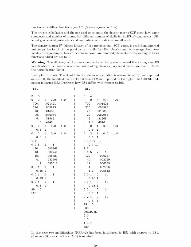
functions, or diffuse functions (see http://www.cryscor.unito.it).

The present calculation and the one used to compute the density matrix SCF guess have samesymmetry and number of atoms, but different number of shells in the BS of some atoms. Dif-ferent geometrical parameters and computational conditions are allowed.

The density matrix P0 (direct lattice) of the previous run, SCF guess, is read from externalunit (copy file fort.9 of the previous run in file fort.20). Density matrix is reorganized: ele-ments corresponding to basis functions removed are removed, elements corresponding to basisfunctions added are set to 0.

Warning. The efficiency of this guess can be dramatically compromised if not congruent BSmodifications, i.e. insertion or elimination of significantly populated shells, are made. Checkthe normalization factor.

Example. LiH bulk. The BS of Li in the reference calculation is referred to as BS1 and reportedon the left, the modified one is referred to as BS2 and reported on the right. The GUESDUALoption following BS2 illustrates how BS2 differs with respect to BS1.

BS1 | BS2

3 3 | 3 40 0 6 2.0 1.0 | 0 0 6 2.0 1.0700. .001421 | 700. .001421220. .003973 | 220. .00397370. .01639 | 70. .0163920. .089954 | 20. .0899545. .31565 | 5. .315651.5 .4946 | 1.5 .4946

0 0 1 0.0 1.0 | 0 0 1 0.0 1.00.5 1. | 0.5 1.

0 2 1 0.0 1.0 | 0 2 1 0.0 1.00.6 1. | 0.6 1.

1 4 | 0 3 1 0. 1.0 0 5 2. 1. | 0.4 1.120. .000267 | 1 540. .002249 | 0 0 5 2. 1.12. .006389 | 120. .0002674. .032906 | 40. .0022491.2 .095512 | 12. .006389

0 0 1 0. 1. | 4. .0329060.45 1. | 1.2 .095512

0 0 1 0. 1. | 0 0 1 0. 1.0.13 1. | 0.45 1.

0 2 1 0. 1. | 0 0 1 0. 1.0.3 1. | 0.13 1.

99 0 | 0 2 1 0. 1.END | 0.6 1.

| 0 2 1 0. 1.| 0.3 1.| 99 0| END

GUESDUAL2 03 3 11 3 1END

In this case two modifications (NFR=2) has been introduced in BS2 with respect to BS1.Complete SCF calculation (IC=1) is required.

90

First modification in Li (formal atomic number NAT=3) basis set, after the third shell(NSH=3), one shell was added (NU=1).Second modification in H (atomic number IA=1) basis set, after the third shell (NSH=3), oneshell (NU=1) was inserted.

GUESSF - Fock/KS matrix from a previous run

Obsolete - See GUESSP, page 91.

GUESSP - SCF guess - Density matrix from a previous run

The density matrix from a previous run, P0 (direct lattice), is read from disk, and used as SCFguess. No input data are required.

The density matrix can be edited to modify the spin state. See SPINEDIT, page 100.

The density matrix used as SCF guess was written with wave function information in file fort.9at the end of a previous SCF run, and read as file fort.20.The two cases, the present one and that used for the restart, must have same symmetry, andsame number of atoms, basis functions and shells. Atoms and shells must be in the same order.The program does not check the 1:1 old–new correspondence.Different geometrical parameters, computational conditions or exponents of the Gaussian prim-itives are allowed.In geometry and/or basis set optimization, this technique will significantly reduce the numberof SCF cycles. The following scheme shows how to proceed.

1. First run to generate the density matrix

Program inp. block section commentscrystal 0 1 Title

1 1.1 geometry input2 1.2 basis set input3 1.3 computational parameters and SCF input

save wf in file fort.9 (binary) or file.98 (formatted)

2. Second run - the density matrix is read in as a guess to start SCF

copy file fort.9 to fort.20 (or convert file fort.98 and then copy)Program inp. block section commentscrystal 0 1 Title

1 1.1 geometry input2 1.2 basis set input3 1.3 computational parameters and SCF input

(GUESSP)

Warning The modification of the geometry may result in a different order in the storage ofthe matrix elements associated to each overlap distribution in the present and the previousrun. To avoid the mismatch it is strongly recommended to classify the integrals of the presentcase using the geometry of the previous case (FIXINDEX, page 86).

Warning When wave function information are stored formatted in file fort.98, the data mustbe converted to binary by the keyword RDFMWF, page 167 of the properties program).Warning SCF guess from a density matrix computed with a different basis set is allowed bythe keyword GUESDUAL, page 89.

GUESSPAT - Superposition of atomic densities

The standard initial guess to start the SCF cycle is the superposition of atomic (or ionic)densities. No input data are required. The electronic configuration of the atoms is entered asa shell occupation number in the basis set input (page 19). Different electronic configurations

91

may be assigned to atoms with the same atomic number and basis set (but not symmetryrelated) through the keyword CHEMOD (page 19).

INTGPACK - Choice of bielectronic integrals package

rec variable value meaning• ∗ IPACK [0] s, sp shells→ POPLE; p, d shells → ATMOL

1 ATMOL for Coulomb integrals;POPLE for exchange integrals

2 POPLE for Coulomb integrals;ATMOL for exchange integrals

3 ATMOL for Coulomb integrals;ATMOL for exchange integrals

By default the bielectronic integrals are computed using a set of routines derived from Pople’sGAUSSIAN 70 package [70], if s and sp shells are involved, and by routines derived fromATMOL [84] for p and d shells. The value of IPACK allows different choices. Integrals involvingp or d shells are always computed by ATMOL. The ATMOL package can compute integrals overfunctions of any quantum number, but the symmetry treatment implemented in the CRYSTALpackage allows usage of s, p and d functions only. The use of sp shells (s and p orbitals sharingthe same exponent) reduces the time required to compute the integrals considerably.

KSYMMPRT

Symmetry Adapted Bloch Functions [138, 137] (page 101)are used as basis for the Fock/KSmatrix diagonalization. The results of the symmetry analysis in reciprocal space are printed.At each k-point: number of point symmetry operators, number of active IRs, maximum IRdimension and maximum block dimension in the Fock/KS matrix factorization. TESTRUNstops execution after this information is printed.No input data required.Extended information can be obtained by setting the value N of LPRINT(47) (keyword SET-PRINT, page 54) before KSYMMPRT.

N information0 Basic Symmetry Information - At each k-point: list of point symmetry operators,

IR dimensions and number of Irreducible Sets.> 0 Symmetry Information - At each k-point ≤ N: class structure, character table

and IR information concerning the K-Little Group. For the rest of the k-pointthe same information as -1 is printed.

< −1 Full Symmetry Information - At each k-point: the same information as N > 0,together with the matrix representatives of the point operators.

MPP doesn’t support KSYMMPRT.

LEVSHIFT - Eigenvalue level shifting

rec variable value meaning• ∗ ISHIFT The level shifter is set to ISHIFT *0.1 hartree.

ILOCK 0 no locking1 causes a lock in a particular state (eg non-conducting) even if the so-

lution during the SCF cycles would normally pass through or even con-verge to a conducting state.

The eigenvalue level shifting technique is well known in molecular studies [62, 29], and mayalso be used for periodic systems. The technique involves the addition of a negative energyshift to the diagonal Fock/KS matrix elements (in the Crystalline Orbital basis) of the occupiedorbitals and thus reducing their coupling to the “unoccupied” set. This shift may be main-tained (ILOCK=1) or removed (ILOCK=0) after diagonalization. The former case causes a

92

lock in a particular state (eg non- conducting) even if the solution during the SCF cycles wouldnormally pass through or even converge to a conducting state.

This option provides an alternative damping mechanism to Fock/KS matrix mixing (FMIX-ING, page 87). The locking is effective only if ISHIFT is large enough. If locking is used, theFermi energy and the eigenvalues are depressed by the value of the level shifter. Suggestedvalues :

1. Normal cases require no mixing of Fock/KS matrices in successive cycles to converge:ISHIFT=0 (default).

2. When 20% to 30% mixing of Fock/KS matrices is necessary, an ISHIFT value of between1 and 3 (giving a level shift of 0.1 to 0.3 hartree) may produce an equivalent or evensuperior convergence rate.

3. If serious convergence difficulties are encountered, ISHIFT=10 will normally be adequate,corresponding to a level shift of 1 hartree. But it may happen that the system movestowards an excited state, and no convergence is obtained.

Warning - Hamiltonian eigenvalues are modified by the level shifter. Take into account whenlooking at top and bottom bands eigenvalues printed.

See tests 29, 30, 31, 32, 38.

MAXCYCLE

rec variable meaning• ∗ NMAX maximum number of SCF cycles [50]

The possibility to modify the maximum number of SCF cycles allows: increasing the numberof cycles in case of very slow convergence (metals, magnetic systems, DFT);The keyword POSTSCF forces saving wave function data in file fort.9, even if SCF endsbefore reaching convergence for ”too many cycles”.

MONSPLIT - Splitting of large monoelectronic integral files

rec variable meaning• ∗ NFILE number of files to be used [1] (max 10)

Very large basis sets can produce billions monoelectronic integrals to be stored, as the numberof monoelectronic integrals scales as the square of basis set size. The multipolar expansiontechnique based on the atoms reduces the disk space up to a factor 3, compared to the valueprinted as estimate. The distribution of the integrals over several disk files may be necessary,if available disk space is limited.

MPP - Massive Parallel Execution - Programmers only

No input data required.

This option is available only with MPPcrystal, the massively parallel version of CRYSTAL09,where Massive Parallel Libraries are linked, and matrices in the reciprocal space are distributedover the processors.

MPPcrystal is designed to compute the total energy and wavefunction of large unit cell systemswith large memory requirements. In particular, The MPP option is eligible when nk/nprocs,i.e. the ratio between nk, the number of k points sampled in the reciprocal space and nprocs,the number of processors used, is small.

In choosing nprocs, the user should consider that MPP is efficient when nAO/nprocs ≥ 50 (nAO

is the number of Atomic Orbitals per cell, or basis functions). If nprocs is too large compared to

93

the size of the system, some parts of the calculation (matrix diagonalization) become inefficientbecause of increasing communications among processors.

Advantages of MPP:

• matrix diagonalization is well balanced because many processors are involved in the di-agonalization of one matrix (use of standard linear algebra libraries for massively parallelcalculation)

• memory requirement per processor decreases with nprocs because data are distributed toprocessors

• I/O is limited to reading the user’s input deck and writing the output files with theresults of a job.

Warnings.

• The following options are not available with MPP:

keyword block

CPHF CPHF 1Frequency calculation - IR intensities FREQCALC/INTENS 1Bloch Functions Symmetry Adapted SYMADAPT 3Printing of eigenvalues of overlap matrix in k space EIGS 3

• use of option NOBIPOLA (page 95) is recommended for very large systems, becausedata distribution has not been implemented for the bipolar approximation of two-electronintegrals (such approximation becomes less efficient with large unit-cell systems so thatswitching to NOBIPOLA does generally not affect performance significantly)

• MPP calculations run with NOSYMADA (page 95) active (no use of symmetry in thereciprocal space)

• keyword DCDIAG may activate Divide&Conquer diagonalization strategy (not default)which improves performance; however, it must be used with caution as one failure wasreported in one case where eigenvectors and eigenvalues were not determined correctly(with no other clear symptom)

• SCF convergence may proceed along slightly different paths with and without MPP,particularly in sensitive cases, and SCF convergence acceleration methods may exhibitdifferent behaviours. A particular setting of convergence tool parameters, for example agiven mixing rate of matrices along several SCF steps, may be either effective or ineffectivewhen using MPP or not. However, a proper choice of the parameters will always resultinto achievement of the SCF cycle convergence.

If keyword MPP is not part of the input deck, MPPcrystal will run as Pcrystal (replicated datastorage in memory, matrix diagonalization by k-point with one full matrix diagonalization perprocessor, no link to external libraries).

MYBIPOLA - Bipolar expansion approximation control

rec variable meaning• ∗ ILCOUL maximum multipole order for Coulomb 4∗ ITCOUL overlap threshold for Coulomb 14∗ IFCOUL reducing factor for Coulomb 90

• ∗ ILEXCH maximum multipole order for exchange 2∗ ITEXCH overlap threshold for exchange 10∗ IFEXCH reducing factor for exchange 70

94

The bipolar approximation is applied in the evaluation of the Coulomb and exchange integrals(page 225). Maximum values for ILCOUL and ILEXCH are 8 and 4, respectively. ITCOUL andITEXCH can be assigned any intermediate value between the default values (14 and 10) (seepage 225) and the values switching off the bipolar expansion (20000 and 20000). IncreasingIFCOUL and IFEXCH the threshold is lightly modified in order to increase the number ofapproximated integrals, and vice versa.

Warning - for developers only

NEIGHBOR/NEIGHPRT


NOBIPOLA - Bipolar expansion approximation suppression

All the bielectronic integrals, coulomb and exchange, are evaluated exactly. The overlap thresh-old both for coulomb and exchange integrals is set to 2000000.No input data required. The CPU time in the integrals program may increase up to a factor3.

NOBIPCOU - Bipolar expansion approximation of coulomb integralssuppression

Coulomb bielectronic integrals are evaluated exactly. The overlap threshold for coulomb inte-grals is set to 2000000.No input data required.

NOBIPEXC - Bipolar expansion approximation of exchange integralssuppression

Exchange bielectronic integrals are evaluated exactly. The overlap threshold for exchangeintegrals is set to 2000000. No input data required.

NOFMWF - Wave function formatted output

CRYSTAL writes the formatted wave function in file fort.98 at the end of SCF by default.This keyword deletes this feature.

NOMONDIR - Monoelectronic integrals on disk

No input data required.In the SCF step bielectronic integrals are computed at each cycle, while monoelectronic inte-grals are computed once and read from disk at each cycle.

NOSYMADA

The Symmetry Adapted Functions are not used in the Hamiltonian matrix diagonalization. Noinput data are required. This choice increases the diagonalization CPU time when the systemhas symmetry operators.

PARAMPRT - - printing of parametrized dimensions


95

POLEORDR - Maximum order of multipolar expansion

rec variable meaning• ∗ IDIPO maximum order of pole [4]

Maximum order of shell multipoles in the long-range zone for the electron-electron Coulombinteraction. Maximum value = 6. See Section 11.3, page 223.

POSTSCF

Calculation to be done after scf (gradient, population analysis) are performed even if conver-gence is not reached. It may be useful when convergence is very slow, and scf ends for ”TOOMANY CYCLES” very close to the convergence criteria required.No input data are required.

PPAN/MULPOPAN - Mulliken Population Analysis

Mulliken population analysis is performed at the end of SCF process.No input data are required.Bond populations are analysed for the first n neighbours (n default value 3; see NEIGHBOR,page 51, to modify the value).Computed data:

1. aµ =∑

ν

∑g P

gµνS

gµν orbital charges

2. sl =∑

µ∈l aµ shell charges

3. qA =∑

l∈A sl atomic charges

4. b(A0, Bg) =∑

µ∈A

∑ν∈B P

gµνS

gµν bond populations between the non-equivalent atoms in

the unit cell (A0) and their first NVI neighbours (Bg in cell g). The printed values mustbe multiplied by 2 when B 6=A to compare with standard molecular calculations.

Formatted data are written in file PPAN.DAT (opened in forrtran unit 24).See Appendix D, page 263.



RHF [default]

A restricted closed-shell hamiltonian calculation is performed ([108, 103], Chapter 8 of ref.[100]). Default choice.

ROHF

Obsolete. See UHF

SCFDIR

No input data required.In the SCF step monoelectronic and bielectronic integrals are evaluated at each cycle. Noscreening of the integrals is performed.

96

SAVEWF

The wave function is written in file fort.79 every two cycles. The format is the same as in filefort.9, written at the end of SCF.To restart SCF cycles using the density matrix written in file fort.79, it has to be copied in filefort.20No input data required.





SHRINK - Pack-Monkhorst/Gilat shrinking factors

rec variable value meaningif the system is periodic insert II

• ∗ IS Shrinking factor in reciprocal space (Section 11.7, page 227)ISP Shrinking factor for a denser k point net (Gilat net) in the

evaluation of the Fermi energy and density matrix.if IS = 0 insert II

• ∗ IS1,IS2,IS3 Shrinking factors along B1,B2,B3 (reciprocal lattice vectors);to be used when the unit cell is highly anisotropic


For periodic systems, 1D, 2D, 3D, the mandatory input information is the shrinking factor, IS,to generate a commensurate grid of k points in reciprocal space, according to Pack-Monkhorstmethod. The Hamiltonian matrix computed in direct space, Hg, is Fourier transformed foreach k value, and diagonalized, to obtain eigenvectors and eigenvalues:

Hk =∑

g

Hgeigk

HkAk = SkAkEk

A second shrinking factor, ISP, defines the sampling of k points, ”Gilat net” [57, 56], usedfor the calculation of the density matrix and the determination of Fermi energy in the case ofconductors (bands not fully occupied).In 3D crystals, the sampling points belong to a lattice (called the Pack-Monkhorst net), withbasis vectors:

b1/is1, b2/is2, b3/is3 is1=is2=is3=IS, unless otherwise stated

where b1, b2, b3 are the reciprocal lattice vectors, and is1, is2, is3 are integers ”shrinkingfactors”.In 2D crystals, IS3 is set equal to 1; in 1D crystals both IS2 and IS3 are set equal to 1. Onlypoints ki of the Pack-Monkhorst net belonging to the irreducible part of the Brillouin Zone(IBZ) are considered, with associated a geometrical weight, wi. The choice of the reciprocalspace integration parameters to compute the Fermi energy is a delicate step for metals. SeeSection 11.7, page 227. Two parameters control the accuracy of reciprocal space integrationfor Fermi energy calculation and density matrix reconstruction:

IS shrinking factor of reciprocal lattice vectors. The value of IS determines the number of kpoints at which the Fock/KS matrix is diagonalized. Multiples of 2 or 3 should be used,according to the point symmetry of the system (order of principal axes).

97

In high symmetry systems, it is convenient to assign IS magic values such that all lowmultiplicity (high symmetry) points belong to the Monkhorst lattice. Although thischoice does not correspond to maximum efficiency, it gives a safer estimate of the integral.

The k-points net is automatically made anisotropic for 1D and 2D systems.

The figure presents the reciprocal lattice cell of 2D graphite (rhombus), the firstBrillouin zone (hexagon), the irreducible part of Brillouin zone (in grey), and the

coordinates of the ki points according to a Pack-Monkhorst sampling, with shrinkingfactor 3 and 6.

ISP shrinking factor of reciprocal lattice vectors in the Gilat net (see [103], Chapter II.6).ISP is used in the calculation of the Fermi energy and density matrix. Its value can beequal to IS for insulating systems and equal to 2*IS for conducting systems.

The value assigned to ISP is irrelevant for non-conductors. However, a non-conductormay give rise to a conducting structure at the initial stages of the SCF cycle, owing, forinstance, to a very unbalanced initial guess of the density matrix. The ISP parametermust therefore be defined in all cases.Note. The value used in the calculation is ISP=IS*NINT(MAX(ISP,IS)/IS), a multipleinteger of IS. For instance:

input data IS ISP ISP for wf calculation3 4 33 6 63 8 6

In the following table the number of sampling points in the IBZ and in BZ is given for afcc lattice (space group 225, 48 symmetry operators) and hcp lattice (space group 194, 24symmetry operators). The CRYSTAL code allows 413 k points in the Pack-Monkhorst net,and 2920 in the Gilat net.

98

IS points in IBZ points in IBZ points BZfcc hcp

6 16 28 1128 29 50 26012 72 133 86816 145 270 205218 195 370 292024 413 793 691632 897 1734 1638836 1240 2413 2333248 2769 5425 55300

1. When an anisotropic net is user defined (IS=0), the ISP input value is taken as ISP1(shrinking factor of Gilat net along first reciprocal lattice) and ISP2 and ISP3 are set to:ISP2=(ISP*IS2)/IS1,ISP3=(ISP*IS3)/IS1.

2. User defined anisotropic net is not compatible with SABF (Symmetry Adapted BlochFunctions). See NOSYMADA, page 95.

Some tools for accelerating convergence are given through the keywords LEVSHIFT (page92 and tests 29, 30, 31, 32, 38), FMIXING (page 87), SMEAR (page 99), BROYDEN(page 73) and ANDERSON (page 71).At each SCF cycle the total atomic charges, following a Mulliken population analysis scheme,and the total energy are printed.The default value of the parameters to control the exit from the SCF cycle (∆E < 10−6 hartree,maximum number of SCF cycles: 50) may be modified entering the keywords:TOLDEE (tolerance on change in total energy) page 102;TOLDEP (tolerance on SQM in density matrix elements) page 102;MAXCYCLE (maximum number of cycles) page 93.

SMEAR

rec variable meaning• ∗ WIDTH temperature smearing of Fermi surface

Modifies the occupancy of the eigenvalues (fj) used in reconstructing the density matrix fromthe step function, (equation 11.9, page 222) to the Fermi function;

fj = (1 + e(εj−εF )

kbT )−1 (2.20)

where εF is the Fermi energy and kbT is input as WIDTH in hartree.

The smearing of the Fermi surface surface may be useful when studying metallic systems inwhich the sharp cut-off in occupancy at εF can cause unphysical oscillations in the chargedensity. It may also result in faster convergence of the total energy with respect to k-pointsampling.

In density functional theory the use of Fermi surface smearing finds a formal justification inthe finite temperature DFT approach of Mermin [83]. In this case the “free energy” of thesystem may be computed as:

F = E(T )− kbTS(T )

= E − kbT

Nstates∑i

fi ln fi + (1− fi) ln(1− fi) (2.21)

where S is the electronic entropy. Often we wish to compute properties for the athermal limit(T=0). For the free electron gas the dependencies of the energy and entropy on temperatureare:

99

E(T ) = E(0) + αT 2

S(T ) = 2αT (2.22)

and so the quantity

E0 =F (T ) + E(T )

2= E(0) +O(T 3) (2.23)

may be used as an estimate of E(0).

0.56

0.58

0.6

0.62

0.64

0.66

0.68

0.7

0.72

0 2 4 6 8 10 12 14 16 18

Using E(T) kT=0.001H ♦

♦

♦

♦

♦ ♦ ♦♦

♦♦ ♦

♦♦

♦ ♦ ♦ ♦♦ ♦

Using E(T) kT=0.02H ++

+ + + + + + + + + + + + + + +

Using E0 kT=0.02H

Figure 2.4: The surface energy (J/M2) of Li(100) for various numbers of layers in a slab modelshowing the effects of WIDTH (0.02H and 0.001H) and the use of E(T) or E0

Figure 2.4 shows the effect of WIDTH on the convergence of the Li(100) surface energy. Despitethe dense k-space sampling (IS=24, ISP=48) the surface energy is rather unstable at lowtemperature (0.001H). There is a significant improvement in the stability of the solution forhigher values of WIDTH (0.02H) but use of E(T) results in a surface energy of 0.643 J/M2

significantly above that obtained by extrapolating E(T) to the T=0 limit (0.573 J/M2). Theuse of E0 at WIDTH=0.02H results in an excellent estimate of the surface energy - 0.576 J/M2.

Note that for conducting systems analytic first derivatives are not fully implemented when thekeyword SMEAR is used. In that case, numerical first derivatives should be computed (seepage 113). For very small value of smearing (around 0.001 hartree) analytical gradients shouldbe reliable in geometry optimization.

SPINEDIT - Editing of the spin density matrix

rec variable meaning• ∗ N number of atoms for which spin must be reversed• ∗ LB, L=1,N atom labels

The spin density matrix from a previous run is edited to generate an approximate guess for anew spin configuration. The sign of the elements of the spin density matrix of selected atomsis reversed. The keyword SPINEDIT must be combined with UHF (input block 3, page 102)or DFT/SPIN (input block 3, page 75) and GUESSP.Example: the anti ferromagnetic solution for the spinel MnCr2O4 can be obtained by calculat-ing the ferro magnetic solution, and using as guess to start the SCF process the density matrixof the ferromagnetic solution with reversed signs on selected atoms.

100

SPINLOCK - Spin-polarized solutions

rec variable meaning• ∗ NSPIN nα-nβ electrons∗ NCYC number of cycles the difference is maintained

The difference between the number of α and β electrons at all k points can be locked at theinput value. The number of α electrons is locked to (N + NSPIN)/2, where N is the totalnumber of electrons in the unit cell; the number of β electrons is locked to (N - NSPIN)/2.NSPIN must be odd when the number of electrons is odd, even when the number of electronsis even.Example. Bulk NiO. If a anti ferromagnetic solution is required, a double cell containing 2NiO units must be considered (test 30). The two Ni atoms, related by translational symmetry,are considered nonequivalent. The number of electron is 72, each Ni ion is expected to havetwo unpaired electrons.

INF95 type of solution corresponding to the spin setting0 anti ferromagnetic ↑ ↓ ↑ ↓4 ferromagnetic ↑ ↑ ↑ ↑

Warning To lock the difference between α and β electrons α and β eigenvalues are forced tobe split. Their printed value is meaningless, until locking is active.

See tests 29, 30, 32, 33, 37, 38.

STOP


SYMADAPT

A computational procedure for generating space-symmetry-adapted Bloch functions, when BFare built from a basis of local functions (AO), is implemented. The method, that applies toany space group and AOs of any quantum number, is based on the diagonalization of Diraccharacters [138, 137].The Symmetry Adapted Functions are used in the Hamiltonian matrix diagonalization. Noinput data are required. This choice reduces the diagonalization CPU time when the systemhas symmetry operators. Default choice.Not supported by MPP execution.

TESTPDIM

The program stops after processing of the full input (all four input blocks) and performingsymmetry analysis. The size of the Fock/KS and density matrices in direct space is printed.No input data are required.It may be useful to obtain information on the neighbourhood of the non equivalent atoms (upto 3, default value; redefined through the keyword NEIGHBOR, input block 1, page 51).

TEST[RUN] - Integrals classification and selection

Full input (geometry, basis set, general information, SCF) is processed.The symmetry analysis is performed, and the monoelectronic and bielectronic integrals classi-fied and selected, according to the the truncation criteria adopted. The size of the Fock/KSand density matrices (direct lattice) and the disk space required to store the bielectronic areprinted. The value printed as ”disk space for monoelectronic integrals” is an upper limit. Thenew technique of atomic multipolar expansion reduces the required space to about 1/3 of theprinted value.

No input data required.

101

This type of run is fast, and allows an estimate of the resources to allocate for the traditionalSCF wave function calculation.

TOLDEE - SCF convergence threshold on total energy

rec variable meaning• ∗ ITOL 10−ITOL threshold for convergence on total energy

Different default values are set for different type of calculation:

SCF single point 6Geometry optimization OPTGEOM 7Frequency calculation FREQCALC 10Elastic constants ELASTCON 8Equation of state EOS 8

TOLDEP - SCF convergence threshold on density matrix

rec variable meaning• ∗ ITOL 10−ITOL threshold for convergence on ∆P

For developers only.

TOLINTEG - Truncation criteria for bielectronic integrals(Coulomb and HF exchange series)

rec variable meaning• ∗ ITOL1 overlap threshold for Coulomb integrals- page 223 6

ITOL2 penetration threshold for Coulomb integrals-page 224 6ITOL3 overlap threshold for HF exchange integrals-page 224 6ITOL4 pseudo-overlap (HF exchange series-page 224) 6ITOL5 pseudo-overlap (HF exchange series-page 224) 12

The five ITOL parameters control the accuracy of the calculation of the bielectronic Coulomband exchange series. Selection is performed according to overlap-like criteria: when the overlapbetween two Atomic Orbitals is smaller than 10−ITOL, the corresponding integral is disregardedor evaluated in a less precise way. Criteria for choosing the five tolerances are discussed inChapter 11.

TOLPSEUD - Truncation criteria for integrals involving ECPs

rec variable meaning• ∗ ITPSE overlap threshold for ECP integrals 6

The program evaluates only those integrals for which the overlap between the charge distri-bution ϕ0

µ ϕgν (page 221) and the most diffuse Gaussian defining the pseudopotential is larger

than a given threshold Tps=10−ITPSE (default value 10−6; it was 5 in CRYSTAL98).

UHF - Hamiltonian for Open Shell Systems

For the description of systems containing unpaired electrons (such as molecules with an oddnumber of electrons, radicals, ferromagnetic and anti ferromagnetic solids) a single determinantis not an appropriate wave-function; in order to get the correct spin eigenfunction of thesesystems, it is necessary to choose a linear combination of Slater determinants (whereas, in

102

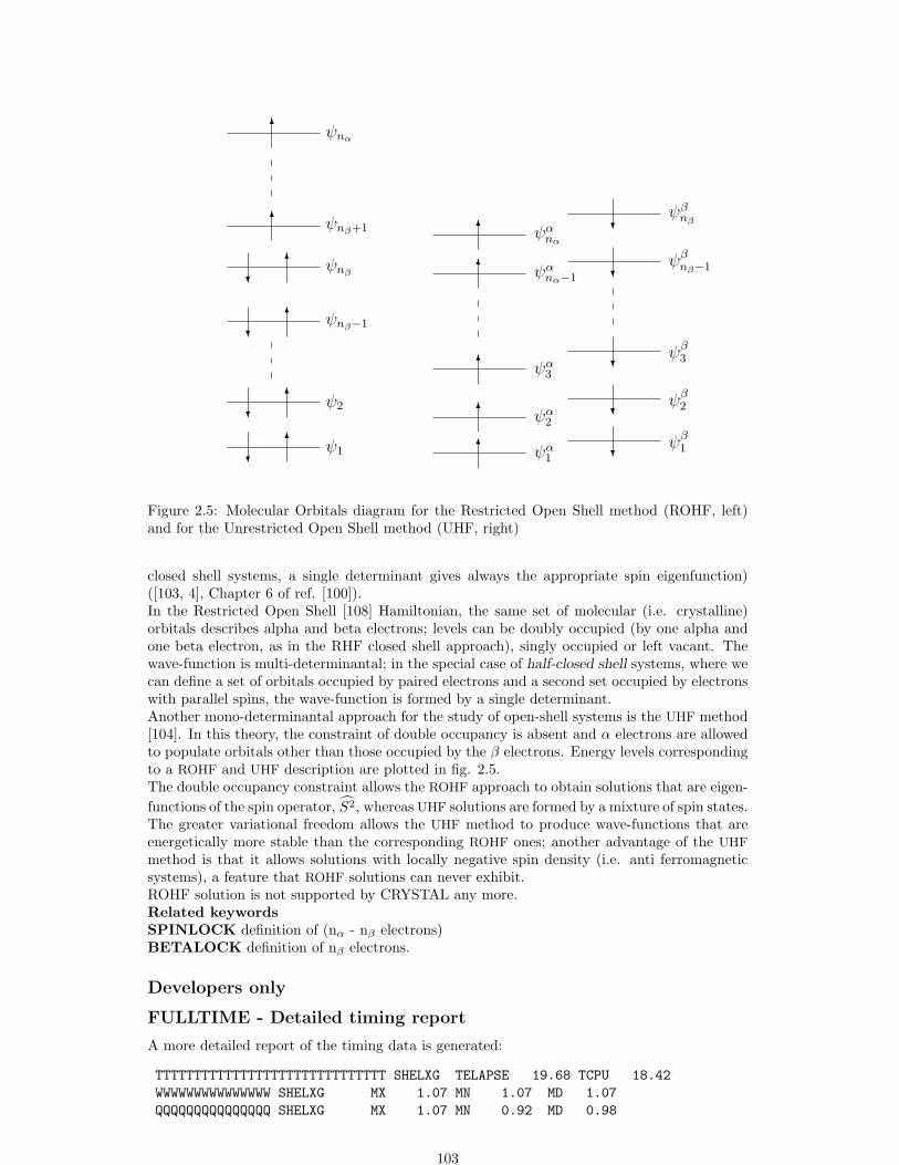
6?

?6

?6

?6

6

6

6

6

6

6

6

?

?

?

?

?

ψ1

ψ2

ψnβ−1

ψnβ

ψnβ+1

ψnα

ψα1

ψα2

ψα3

ψαnα−1

ψαnα

ψβ1

ψβ2

ψβ3

ψβnβ−1

ψβnβ

Figure 2.5: Molecular Orbitals diagram for the Restricted Open Shell method (ROHF, left)and for the Unrestricted Open Shell method (UHF, right)

closed shell systems, a single determinant gives always the appropriate spin eigenfunction)([103, 4], Chapter 6 of ref. [100]).In the Restricted Open Shell [108] Hamiltonian, the same set of molecular (i.e. crystalline)orbitals describes alpha and beta electrons; levels can be doubly occupied (by one alpha andone beta electron, as in the RHF closed shell approach), singly occupied or left vacant. Thewave-function is multi-determinantal; in the special case of half-closed shell systems, where wecan define a set of orbitals occupied by paired electrons and a second set occupied by electronswith parallel spins, the wave-function is formed by a single determinant.Another mono-determinantal approach for the study of open-shell systems is the UHF method[104]. In this theory, the constraint of double occupancy is absent and α electrons are allowedto populate orbitals other than those occupied by the β electrons. Energy levels correspondingto a ROHF and UHF description are plotted in fig. 2.5.The double occupancy constraint allows the ROHF approach to obtain solutions that are eigen-functions of the spin operator, S2, whereas UHF solutions are formed by a mixture of spin states.The greater variational freedom allows the UHF method to produce wave-functions that areenergetically more stable than the corresponding ROHF ones; another advantage of the UHF

method is that it allows solutions with locally negative spin density (i.e. anti ferromagneticsystems), a feature that ROHF solutions can never exhibit.ROHF solution is not supported by CRYSTAL any more.Related keywordsSPINLOCK definition of (nα - nβ electrons)BETALOCK definition of nβ electrons.

Developers only

FULLTIME - Detailed timing report

A more detailed report of the timing data is generated:

TTTTTTTTTTTTTTTTTTTTTTTTTTTTTT SHELXG TELAPSE 19.68 TCPU 18.42WWWWWWWWWWWWWWW SHELXG MX 1.07 MN 1.07 MD 1.07QQQQQQQQQQQQQQQ SHELXG MX 1.07 MN 0.92 MD 0.98

103

The first line is the standard data. The second line reports the minimum, maximum and meanwall time since the last report. The last line reports the minimum, maximum and mean cputime since the last report. The minimum, maximum and mean operations are across processors,and so this directive is most useful for parallel job.

DCDIAG - ”divide and conquer” diagonalization

This directive is ONLY for MPP jobs. It instructs the code to use the divide and conqueralgorithm for the diagonalization stage. This algorithm can be up to four times quicker thanthe standard, but it has been found very, very, occasionally to generate incorrect results.

CMPLXFAC - Detailed timing report

This directive is ONLY for MPP jobs. For load balancing reasons the MPP code must knowhow many times more expensive a calculation on a complex k point is relative to a real one.This allows the user to specify a value for this. The default value is 2.333333.

QVRSGDIM - limiting size switch for multipole moments gradients

rec variable meaning• ∗ NFILE limiting size of multipole moment gradients to switch from generation by

pairs to generation by shells. Default 90000000.

104

Chapter 3

Geometry optimization

Geometry optimization at constant symmetry is invoked by the keyword OPTGEOM in inputblock 1 (geometry). OPTGEOM must be the last keyword in geometry input. OPTGEOMinput block admits several options (sub keywords), and terminates with keyword END (orEND[OPT], END[—]: the first three characters only are processed).

crystal allows geometry optimization of systems with any periodicity: molecules, polymers,slabs, and crystals. Unconstrained relaxation of the structure and different optimizations withconstraints can be carried out. The full symmetry of the system is preserved.

Geometry optimization can be performed in symmetrized fractional coordinates [default] orredundant internal coordinates (optional choice, page 115).

OPTGEOM sub keywords can be classified as follow:

1. General sub keywords:

A - Optimization type (page 109)B - Initial Hessian (page 109)C - Hessian updating technique (page 107)D - Convergence criteria (page 106)E - Step control (page 110)F - Coordinate system related options (page 111)G - Optimization procedure control (page 112)H - Numerical (first) derivatives (page 113)I - Printing options (page 114)

2. Geometry optimization in redundant coordinates (page 115).

3. Geometry optimization with constraints (page 117).

A - Constant volume optimization (page 117)B - Fixing lattice deformations (page 118)C - Linear constraints between atomic coordinates (page 119)D - Partial optimization of atomic positions (page 119)E - Fixing internal coordinates (page 120)

4. Geometry optimization with application of an external stress (page 121)

5. Searching a transition state (page 123)

Default values are supplied for all computational parameters.

By default an unconstrained geometry optimization of the atomic positions at fixedcell is performed.

Users can find supplementary information and input examples in the CRYSTAL TutorialsProject web page at the CRYSTAL web site (http://www.crystal.unito.it/tutorials).

105

Geometry optimization strategy

A Quasi-Newton optimization scheme is implemented. Gradients are evaluated every time thetotal energy is computed; the second derivative matrix (i.e. Hessian matrix) is built from thegradients. The default choice for the initial Hessian matrix is obtained from a model Hessian,as proposed by Schlegel and updated by using the BFGS algorithm[19, 20, 50, 59, 120].

By default the step considered is the Newton step (direction and length) controlled by theTrust Radius scheme (see ALLOWTRUSTR page 111). NOTRUSTR to remove trustradius control (CRYSTAL06 default choice).

HF and DFT (pure and hybrid functionals) analytical gradients are used for insulators andconductors, both for all-electron and ECP calculations.Note that for conducting systems analytic first derivatives are not fully implemented whenthe keyword SMEAR (page 99) is used. In that case, numerical first derivatives should becomputed (see page 113).For very small value of smearing (around 0.001 hartree) analytical gradients can be used.

For atomic positions, geometry optimization is performed in symmetrized fractional coordi-nates, in order to exploit the point group symmetry of the lattice. The keyword PRSYMDIR(input block 1, page 53) may be used to print the so-called symmetry allowed directions adoptedin the geometry optimization. If there are no symmetry allowed directions, the program printsa warning message and stops, unless FULLOPTG or CELLONLY is requested (see page109).

To optimize the lattice parameters a set of symmetry preserving cell deformations (see Symme-try Allowed Elastic Distortions, USESAED, page 61) related to changes of isotropic volumeand of axial ratios is defined. By default, the symmetry allowed deformations are printed inthe output file.

When a full optimization of atom positions and cell parameters is carried out, a normalizedcombined set of symmetrized directions and deformations is adopted.

Optional choice (keyword INTREDUN, page 115) is the geometry optimization in redundantinternal coordinates. In such a case, atomic displacements and cell deformations are implicitlydetermined by the internal coordinate system.

Default choices

- Type of optimization:

The default geometry optimization type is the relaxation of the nuclear coordinates at fixedlattice parameters in symmetrized fractional coordinates.Optional choices: see page 109.

- Convergence criteria

A stationary point on the potential energy surface is found when the forces acting on atoms arenumerically zero. Geometry optimization is usually completed when the gradients are below agiven threshold.

In crystal, the optimization convergence is checked on the root-mean-square (RMS) and theabsolute value of the largest component of both the gradients and the estimated displacements.When these four conditions are all satisfied at a time, optimization is considered complete.

In some cases (see page. 123), the optimization process stops with a warning message controlledby the threshold in the energy change between consecutive optimization steps.

Default values are set for all computational parameters, and they may be modified throughkeywords. Default choices:

106

default keyword

RMS on gradient 0.000300 a.u. TOLDEGlargest component of gradient 1.5 * 0.000300 1.5 * TOLDEGRMS on estimated displacements 0.0012 a.u. TOLDEXabsolute value of largest displacement 1.5 * 0.0012 1.5 * TOLDEXmax number of optimization cycles 100 MAXCYCLEenergy change between optimization steps threshold 10−7a.u. TOLDEE

Optimization convergence criteria are set to different values according to the context wheregeometry optimization is performed.

RMS on gradient RMS on displacementStandard geometry opt 0.0003 0.0012preopt in frequency calculation 0.00003 0.00012preopt in EOS 0.00006 0.00012preopt in elastic constants 0.00006 0.00012

- Initial Hessian guess

The initial Hessian is generated by means of a classical model as proposed by Schlegel.

H.B. Schlegel, Theoret. Chim. Acta 66 (1984) 333J.M. Wittbrodt and H.B. Schlegel, J. Mol. Struct. (Theochem) 398-399 (1997) 55

It adopts a simple valence force field. Empirical rules are used to estimate the diagonal forceconstants for a set of redundant internal coordinates (stretches, bends and torsions). Parame-ters are available from H to At.

Warning - To define bonds the sum of covalent radii (see page 53) is used. For ionic systemsit may be necessary to modify the default values (see RAYCOV, page 53).

- Hessian updating technique

BFGS Broyden-Fletcher-Goldfarb-Shanno scheme [19, 20, 50, 59, 120].

Optional choices:

1. Schlegel’s updating scheme [117], (OLDCG, page 110), optimization scheme as in CRYS-TAL03

2. Powell’s updating scheme (POWELL, page 110)

- SCF convergence and guess

The default value for SCF convergence criterion on total energy is set to 10−7 (TOLDEE ininput block 3 to modify it: never reduce accuracy).

After the first step, at each SCF cycle, the density matrix is recovered from the previousgeometry optimization step (implicit GUESSP, page 91 option).

This choice may be modified by inserting the keyword NOGUESS. A superposition of atomicdensities is then adopted on each step as SCF initial guess.

If the SCF solution at a given optimization step does not correspond to real convergence,but to an energy stabilization due to the techniques applied to help convergence (LEVSHIFT,FMIXING, BROYDEN..), the hamiltonian eigenvalues may be unphysical, and there is nochance to recover the SCF process. In those cases it may be better to use an atomic guess(keyword NOGUESS).

107

- Output files

The following formatted files are written during geometry optimization, and may be saved forfurther processing.

fort.33 Cartesian coordinates of the atoms in the unit cell and total energy for each geometryoptimization step are written to file fort.33 in a simple xyz format (see Appendix D, page262). This file is suitable to be read by molecular graphics programs (e.g. Molden...) todisplay the animation of a geometry optimization run.

fort.34 If optimization is successful, the last geometry in written in file fort.34 (format de-scribed in Appendix D, page 264).

The file can be read to define the basic geometry input. See EXTERNAL, page 15

opta(c)xxx At each xxx optimization step, the geometry is written in file optaxxx (opti-mization of atoms coordinates only), or optcxxx (optimization of cell parameters or fulloptimization) in the format of ”fort.34” file (see Appendix D, page 264). The file mustbe renamed ”fort.34” if used to enter geometry input (keyword EXTERNAL).

The ”history” of the optimization allows restarting from a given step with differentparameters, when the procedure did not converge.

OPTINFO.DAT contains information to restart optimization. (see keyword RESTART inOPTGEOM input block, page 113).

HESSOPT.DAT The hessian matrix is written, and can be read to define the initial guessfor the Hessian (keyword HESSOPT) in geometry optimization of a system with samegeometry and symmetry (it may have different BS, Hamiltonian, computational param-eters).

SCFOUT.LOG SCF and optimization process printout is routed to file SCFOUT.LOG afterthe first cycle. Keyword ONELOG: full printing on standard output.

1 - General sub keywords

A number of optional keywords allow tuning of the optimization procedure.

A - Type of optimization (page 109)

B - Initial Hessian (page 109)

C - Hessian updating technique (page 110)

D - Convergence criteria (page 106)

E - Step control (page 110)

F - Coordinate system related options (page 111)

G - Optimization procedure control (page 112)

H - Numerical first derivatives (page 113)

I - Printing options (page 114)

108

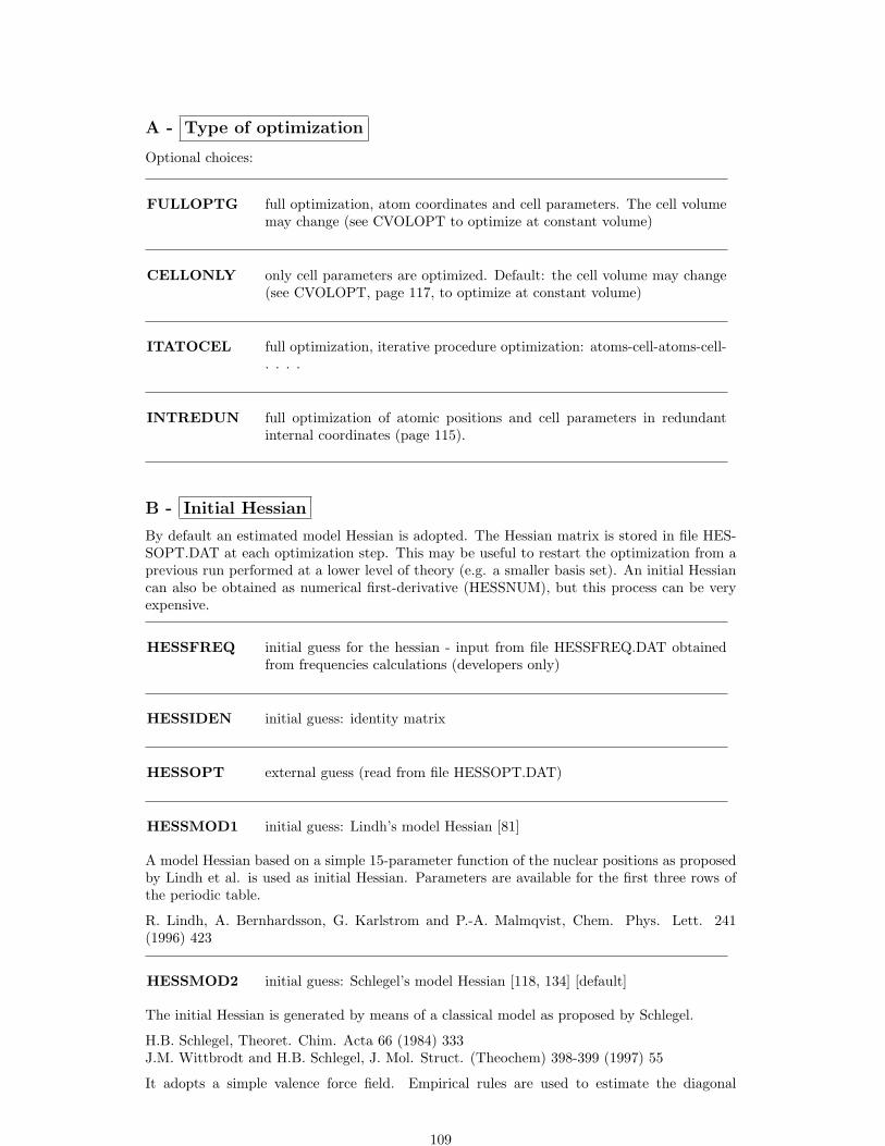
A - Type of optimization

Optional choices:

FULLOPTG full optimization, atom coordinates and cell parameters. The cell volumemay change (see CVOLOPT to optimize at constant volume)

CELLONLY only cell parameters are optimized. Default: the cell volume may change(see CVOLOPT, page 117, to optimize at constant volume)

ITATOCEL full optimization, iterative procedure optimization: atoms-cell-atoms-cell-. . . .

INTREDUN full optimization of atomic positions and cell parameters in redundantinternal coordinates (page 115).

B - Initial Hessian

By default an estimated model Hessian is adopted. The Hessian matrix is stored in file HES-SOPT.DAT at each optimization step. This may be useful to restart the optimization from aprevious run performed at a lower level of theory (e.g. a smaller basis set). An initial Hessiancan also be obtained as numerical first-derivative (HESSNUM), but this process can be veryexpensive.

HESSFREQ initial guess for the hessian - input from file HESSFREQ.DAT obtainedfrom frequencies calculations (developers only)

HESSIDEN initial guess: identity matrix

HESSOPT external guess (read from file HESSOPT.DAT)

HESSMOD1 initial guess: Lindh’s model Hessian [81]

A model Hessian based on a simple 15-parameter function of the nuclear positions as proposedby Lindh et al. is used as initial Hessian. Parameters are available for the first three rows ofthe periodic table.

R. Lindh, A. Bernhardsson, G. Karlstrom and P.-A. Malmqvist, Chem. Phys. Lett. 241(1996) 423

HESSMOD2 initial guess: Schlegel’s model Hessian [118, 134] [default]

The initial Hessian is generated by means of a classical model as proposed by Schlegel.

H.B. Schlegel, Theoret. Chim. Acta 66 (1984) 333J.M. Wittbrodt and H.B. Schlegel, J. Mol. Struct. (Theochem) 398-399 (1997) 55

It adopts a simple valence force field. Empirical rules are used to estimate the diagonal

109

force constants for a set of redundant internal coordinates (stretches, bends and torsions).Parameters are available from H to At.

Warning - To define bonds the sum of covalent radii (see page 53) is used. For ionic systemsit may be necessary to modify the default values (see RAYCOV, page 53).

HESSNUM initial guess: numerical estimate

C - Hessian updating technique

Different Hessian updating schemes are available for minimization:

BFGS Hessian update - Broyden-Fletcher-Goldfarb-Shanno scheme [19, 20, 50,59, 120] - [default]

OLDCG Hessian updating - old Schlegel updating scheme[117] (CRYSTAL03)

POWELL Hessian update - symmetric Powell scheme [105]

D - Optimization convergence criteria

These options are available to modify the default values:

TOLDEE threshold on the energy change between optimization steps• ∗ IG |∆E| < 10−IG (default: 7)

The value of IG must be larger or equal to the threshold adopted for the SCF convergence.The value is checked when input block 3, defining the SCF convergence criteria, is processed.

TOLDEG convergence criterion on the RMS of the gradient• ∗ TG max RMS of the gradient (default: 0.0003)

TOLDEX convergence criterion on the RMS of the displacement• ∗ TX max RMS of the displacement (default: 0.0012)

E - Step control

To avoid the predicted step size being too large, two options are available:

Simple scalingSimple scaling of the displacement vector. Each component is scaled by a factor that makesthe largest component of the displacement vector equal to 0.5 a.u.

Trust Radius [default]A more sophisticated and accurate technique to control the step size is the trust radius region

110

scheme. The trust radius limits the step length of the displacement at each cycle, accordingto the quadratic form of the surface in the actual region. The default maximum value forminimization is 0.5.

To run CRYSTAL06 as CRYSTAL09 the keyword ALLOWTRUSTR must be specified alongwith BFGS.

To run CRYSTAL09 as CRYSTAL06, the keyword NOTRUSTR must be specified in geom-etry optimization input

Related keywords are discussed below:

ALLOWTRUSTR activate the trust radius technique to control the step size [0.5 for geometryoptimization; 0.1 for transition state search] [default]

The step at each cycle is computed by means of a Newton-like scheme, while the length isdetermined by linear minimization along an extrapolated quadratic polynomial.

MAXTRADIUS optional• ∗ TRMAX maximum value allowed for the trust radius - default [16]

This is useful in transition state optimizations or in minimizations along flat potential surfacesin order to avoid too large displacements from one point to the next one. Default value:geometry optimization: ∞ ; transition states search : 0.3

NOTRUSTR not using trust radius to limit displacement

TRUSTRADIUS• ∗ TRADIUS set the initial value for trust radius

Set the initial value of the trust radius to [TRADIUS]. The trust radius limitates the steplength of the displacement at each cycle, according to the quadraticity of the surface in theactual region.Default: geometry optimization 0.5; transition state search 0.1.

Warning - When the Trust Radius technique is active, the value of the trust radius couldbecome too small and the geometry optimization process stops with an error message:”TRUST RADIUS TOO SMALL”.In this case, we suggest to restart the optimization from the last geometry, written to fileoptc(a)xxx, being xxx the optimization cycle number.

F - Coordinate system related options

Geometry optimization can be performed in fractional (default) or redundant internal coor-dinates (see INTREDUN). Default fractional coordinates are defined as symmetry alloweddirections (atomic positions) and deformations (cell). The latter are related to changes ofisotropic volume and of axial ratios.

Some options related to the choice of the coordinate systems are also available:

111

CRYDEF crystallographic-like symmetrized cell deformations, corresponding tosymmetrized strains of the unit-cell edges (consistent with symmetry).This set of deformations is useful for fixing lattice parameters in con-strained optimizations in combination with the keyword FIXDEF (page118) - 3D only.

FRACTION optimization in fractional coordinates

FRACTIOO optimization in normalized fractional coordinates [default when FUL-LOPTG is requested]

FRACTCOOR third type of symmetrized fractional coordinates (non-orthogonal; the ori-gin on polar axes must be explicitly fixed by the FIXCOOR option [to beused with constraints])

RENOSAED renormalize symmetry allowed deformations [default when FULLOPTGis requested]

G - Optimization procedure control

EXPDE• ∗ DE expected energy change used to estimate the initial step [default 10−3 Ha,

if model 1 initial hessian; 10−4 Ha, otherwise]

FINALRUN action after geometry optimization - integrals classification is based on thelast geometry. See page 122

• ∗ ICODE Action type code:0 the program stops (default)1 single-point energy calculation2 single-point energy and gradient calculation3 single-point energy and gradient calculation - if convergence criteria on

gradients are not satisfied, optimization restarts4 step 3 is iterated until full stable optimization

FIXDELTE• ∗ IE 10−ie hartree: threshold on the total energy change for redefining the

geometry to which integral classification is referred - see FIXINDEX,page 86 - [default -1000, no reclassification]

FIXDELTX• ∗ DX RMS (bohr) of the displacement for redefining the geometry to which

integral classification is referred - [default: -1, no reclassification]

112

FIXDEIND the reference geometry for integrals classification does not change duringoptimization [default choice]

FITDEGR• ∗ N degree of polynomial fitting function for linear search:

2 parabolic fit [default]3 cubic polynomial function4 constrained quartic fitting

HESEVLIM limits for the allowed region of hessian eigenvalues (hartree)• ∗ VMIN lower limit [default 0.001]

VMAX upper limit [default 1000.]

ITACCONV• ∗ DE energy difference threshold for ITATOCEL [default 0.1 * TOLDEE be-

tween 2 optimization cycles]

MAXITACE• ∗ MAXI max number of iteration cycles in atom/cell iterative optimization [default

100]

MAXCYCLE• ∗ MAX maximum number of optimization steps [default 100]

N.B. When optimization is restarted, the first restarted optimization cycle number is the lastof the previous run + 1. Set MAXCYCLE value accordingly.

NOGUESS SCF guess at each geometry point: superposition of atomic densities ateach SCF calculation (default choice in geometry optimization: GUESSP

NRSTEPS• ∗ DE number of stored steps to be used in the OLDCG Hessian updating scheme

[default: number of degrees of freedom]

RESTART restart geometry optimization from a previous run.See page 123

SORT sorting of the previous optimization steps information when the OLDCGscheme is active [default:nosort]

H - Numerical first derivatives

The nuclear coordinate gradients of the energy can also be computed numerically. A three-pointnumerical derivative formula is adopted. A finite positive (and then negative) displacement

113

is applied to the desired coordinate and a full SCF calculation is performed. The gradient isthen computed as

gi =E∆xi − E−∆xi

2 ∆xi

where ∆xi is the finite displacement along the i-coordinate.

Such a computation is very expensive compared to analytical gradients, since the cost is 2 ·N ·t,where N is the number of coordinates to be optimized and t the cost of the SCF calculation.Numerical first-derivatives should be avoided whenever possible, but sometimes they are theonly way to obtain gradients (i.e. for metals) and therefore to optimize the atoms coordinates.

One choice only, NUMGRCEL, NUMGRATO, NUMGRALL, is allowed.

NUMGRALL geometry optimization - numerical atomic and cell gradient

NUMGRATO geometry optimization - numerical atomic gradients

NUMGRCEL geometry optimization - numerical cell gradients

STEPSIZE modify step for numerical gradient [default 0.001 au] (developers only)• ∗ STEP new stepsize value

I - Printing options

ONELOG This causes all output to be sent to the standard log file, instead of toSCFOUT.LOG

NOXYZ printing of cartesian coordinates at the end of optimization removed

NOSYMMOPS printing of symmetry operators at the end of optimization removed

PRINTFORCES printing atomic gradients

PRINTHESS printing Hessian information

PRINTOPT prints information on optimization process

PRINT verbose printing

114

2 - Optimization in redundant internal coordinates

INTREDUN geometry optimization in internal redundant coordinates

An optimization in redundant internal coordinates is performed when the keywordINTREDUN is inserted in OPTGEOM input block.

Optional keywords related to geometry optimization in redundant internal coordinates mustfollow.

A symmetrized set of internal coordinates (i.e. bonds, angles and torsions) is defined, whichcontains more coordinates than the requisite internal degrees of freedom.

Redundant internal coordinates are generated according to a hierarchical scheme: bondlengths are firstly identified by using covalent radii. Then, angles are determined on the basisof the irreducible set of distances and, finally, dihedral angles are defined. Note that to definebonds the sum of covalent radii (see page 53) is used. For ionic systems it may be necessaryto reduce the default values (see RAYCOV, page 53). In case of systems constituted byunconnected fragments (ie some molecular crystals or adsorption complexes), fragments arelinked to each other by pseudo “bond lengths” between the closest pair of atoms belonging toeach fragment.

There has been substantial controversy in recent years concerning the optimal coordinatesystem for optimizations.

For molecular systems, it is now well-established that redundant internal coordinates requirefewer optimization steps than Cartesian coordinates. However, this is not definitely demon-strated for periodic systems. Nevertheless, the use of internal coordinates can be very useful inseveral respects: for a chemical intuitive view (e.g. internal coordinates can easily be added),for constrained geometry optimization (see below) and for searching transition states (underdevelopment).

By default, optimization of internal redundant coordinates involves both atomic positions andcell parameters. To avoid optimizing cell parameters the keyword FIXCELL page 116 mustbe specified.

Before running a geometry optimization in redundant internal coordinates, the set of coordi-nates generated automatically by CRYSTAL should be checked for consistency. This can bedone by specifying the keyword TESTREDU.

Optional keywords related to the geometry optimization in redundant internal coordinates arelisted below.

Managing with almost linear angles

Linear or almost linear angles (i.e. close to 1800) can lead to numerical instabilities in thecomputation of the dihedrals. To avoid this problem a common practice is to split the anglein two ones. The double angles are defined by the angles obtained by projection of the vectorsonto two suitable perpendicular planes, in order to avoid the indetermination around 1800. Thethreshold value, beyond which the almost linear angle is split, is controlled by the keywordANGTODOUBLE.

115

ANGTODOUBLE minimum value (degrees) beyond which a double angle is defined• ∗ AL value of the angle (degrees) - default [1650]

The default value is set to 1650. This means that all angles larger than 1650 are automaticallysplit into two.This option can be required, for instance, when optimizing zeolitic structures where siloxanebridges could change a lot during the geometry minimization. In that case, it is better toreduce the default value to 1500.

A list of angle to be converted into two can also be explicitly given by specifying

DBANGLIST list of angles chosen to be converted in double angles - advanced option• ∗ MU number of angles to convert in double• ∗ (IN(I),

I=1,MU)list of the angles

This keyword provides the list of angles chosen to be converted in double angles (i.e. definedby the angles obtained by projection of the vectors onto two suitable perpendicular planes) inorder to avoid the indetermination around 180 degrees). The labels used for the angles arethose provided by a previous automatic generation of internal coordinates computed in a testrun (TESTREDU keyword).

Adding internal coordinates - bonds and angles

When some relevant internal coordinates are missing (e.g. intermolecular bonds) they can beadded by means of two keywords: DEFLNGS and DEFANGLS.

DEFLNGS definition of bond lengths• ∗ NL number of bonds to be added

insert NL sets of 5 data to define the bond AB IILA label of the atom A (it must be in the reference cell)LB label of the atom BI1, I2, I3 indices of the cell where the atom B is located

DEFANGLS definition of bond angles• ∗ NL number of angles to be defined

insert NL sets of 9 data to define the angle ABC IILA label of the atom A (it must be in the reference cell)LB label of the atom BI1, I2, I3 indices of the cell where the atom B is locatedLC label of the atom CI1, I2, I3 indices of the cell where the atom C is located

Other optional keywords

FIXCELL keep cell parameters fixed in internal coordinates optimization

116

STEPBMAT step used for numerical bmat calculation (developers only)• ∗ I integer - step = 10I (default 7: step=107)

TESTREDU request test run for checking automatic definition of internal coordinates.

TOLREDU tolerance used to eliminate redundancies (developers only)• ∗ I tolerance 10−I (default: 7, 10−7).

3 - Geometry optimization with constraints

Along with an unconstrained relaxation of the crystalline structure, options are available toperform different optimizations with constraints.In particular:

A - Constant volume optimization (page 117)

B - Fixing lattice deformations (page 118)

C - Linear constraints between atomic coordinates (page 119)

D - Partial optimization of atomic positions (page 119)

E - Fixing internal coordinates (page 120)

All constraining strategies are compatible with any choice of coordinate system adopted for theoptimization process to perform the optimization process. On the other hand, option E is onlyoperative together with the choice of a redundant internal coordinate system (INTREDUNpage 115).The examples at the CRYSTAL Tutorial Project web page illustrate the use of the availablekeywords for constrained geometry optimizations.

A - Constant volume optimization

CVOLOPT constant volume optimization.

Only active with CELLONLY (cell parameters only optimization) or FULLOPTG (atomcoordinates and cell parameters optimization).The volume is kept fixed at the value corresponding to the input unit cell; all cell angles andratios between cell edges unconstrained by the point-group symmetry are optimized.Examples: in the tetragonal symmetry, only the c/a ratio, and in the monoclinic symmetrythe a/b and b/c ratios and the beta angle, respectively, are optimized.

This option is useful for computing E vs V curves point-by-point by relaxing the crystallinestructure at different values of the cell volume. In this case, the keyword FIXINDEX must beused to obtain a smooth curve. The reference geometry must correspond either to the smallestvolume to be explored, or to the equilibrium structure obtained from a prior optimization run(FULLOPTG).

Warning: if large changes of the individual unit-cell parameters occur in the optimizationprocess, the linear strain approximation may not be strictly obeyed and very small volumevariations (of the order of 0.01%) may ensue.

117

B - Fixing lattice deformations

Linear constraints between unit cell deformations can be set up during optimization by meansof the keyword FIXDEF:

FIXDEF optimization with constrained symmetrized cell deformation - 3D only• ∗ NFIXC number of constraints relating pairs of cell deformations

insert NFIXC records II• ∗ LA,LB integer sequence number of the two constrained symmetrized cell defor-

mations.CA,CB real coefficients multiplying the two cell deformations in the linear com-

bination constraint. If LA=0, the cell deformation denoted by the secondinteger (LB) is kept fixed during the optimization (the coefficients in thiscase can take any value).

FIXDEF can also be combined with the keyword CRYDEF, that sets crystallographic-likecell deformations (i.e. a, b, c, α, β, γ) to fix lattice parameters. Integer sequence number givenas input refer to the minimal set of lattice parameters:

1 2 3 4 5 6cubic ahexagonal a, crhombohedral hexagonal cell a, c

rhombohedral cell a, αtetragonal a, corthorhombic a, b, cmonoclinic a, b, c, β

a, b, c, γa, b, c, α

triclinic a, b, c, α, β, γ

Note that the labels of the symmetry allowed deformations must correspond to the onesprinted in the output file.

As an example, a constrained optimization of the crystalline structure of α-quartz (hexagonal)with the c unit cell edge kept fixed follows

QUARTZ ALFA STO-3GCRYSTAL0 0 21540 0 164.916 5.4054214 0.4697 0. 0.8 0.4135 0.2669 0.1191

OPTGEOMFULLOPTGCRYDEFFIXDEF10 2 0.0 0.0 : the second lattice parameter, c, is kept fixedENDOPTEND

118

C - Linear constraints between atomic coordinates

Linear constraints between atomic coordinates can be set up during optimization by using thekeyword FIXCOOR.

FIXCOOR optimization with constrained symmetrized coordinates• ∗ NFIX number of constraints relating pairs of coordinates

insert NFIX records II• ∗ LA,LB integer sequence number of the two constrained symmetrized coordinates

(sequence numbers are read from the output of PRSYMDIR)CA,CB real coefficients multiplying the two coordinates in the linear combination

constraint. If LA=0, the coordinate denoted by the second integer (LB)is kept fixed during the optimization (the coefficients in this case can takeany value).

Note that the labels of the symmetry allowed directions must correspond to the one printedin the output file (PRSYMDIR keyword for coordinates).

In the following example on α-quartz, two constraints are set up on coordinates

QUARTZ ALFA - Linear constraints between atomic coordinatesCRYSTAL0 0 21540 0 164.916 5.4054214 0.4697 0. 0.8 0.4135 0.2669 0.1191

OPTGEOMFULLOPTGFRACTCOORFIXCOOR22 3 1.0 1.00 4 0.0 0.0ENDOPTEND

1. The x and y fractional coordinates of Oxygen are forced to change by the same amount,so that their difference remains constant.

2. The z coordinate of Oxygen is kept fixed.

In general, any of the structural parameters can be kept fixed in the optimization process bythe combined use of FIXCOOR and FIXDEF keywords.

D - Partial optimization of atomic positions

FRAGMENT Partial geometry optimization (default: global optimization)• ∗ NL number of atoms ”free”• ∗ LB(L),L=1,NL label of the atoms to move

119

Optimization is limited to an atomic fragment. Symmetrized cartesian coordinates are gen-erated according to the list of atoms allowed to move. Note that no advantage is taken inthe gradient calculation to reduce the number of atoms, i.e. gradients are calculated on thewhole system. The symmetrized forces are then computed by using the new set of symmetrizedcoordinates. See example in section 9.4, page 206.

E - Fixing internal coordinates

Constraints on internal coordinates can be easily imposed during geometry optimization.The following two options allow users to both define and freeze one or more bond lengths orangles:

LNGSFROZEN explicitly freezes bond lengths• ∗ MU number of bond lengths to freeze

insert NL sets of 5 data to define the bond AB IILA label of the atom A (it must be in the reference cell)LB label of the atom BI1, I2, I3 indices of the cell where the atom B is located

ANGSFROZEN definition of bond angles to be frozen• ∗ NL number of angles to be frozen

insert NL sets of 9 data to define the angle ABC IILA label of the atom A (it must be in the reference cell)LB label of the atom BI1, I2, I3 indices of the cell where the atom B is locatedLC label of the atom CI1, I2, I3 indices of the cell where the atom C is located

According to the list of redundant internal coordinates automatically generated by the code,bond lengths or angles can also be frozen by means of the FREEZINT option:

FREEZINT freeze internal coordinates (active with INTREDUN only):• ∗ NB first NB bond length are frozen

NA first NA bond angles are frozenND first ND dihedral angles are frozen (not active)

The list of redundant coordinates can be obtained from a prior run, by inserting the keywordTESTREDU (the program stops after printing internal coordinates).

Note that for a better control over the selected frozen internal coordinates we suggest usingthe keywords LNGSFROZEN and ANGSFROZEN.

Constraint optimization combining internal coordinates and fractional coordinates can also beperformed.

For instance, one can keep fixed a bond angle together with the constraint that the x and yfractional coordinates of a given atom change by the same amount. Such a combination ofconstraining strategies must be used with caution, as it may lead to undesired behavior in theoptimization process.

The constraining of internal coordinates is performed with numerical techniques (particu-larly in the back-transformation from redundant internal to cartesian coordinate systems)

120

and the fixed values may be affected by some small changes (in general of the order of 10−4 au).

The following example corresponds to a rigid tetrahedral geometry optimization of α-quartz:

QUARTZ ALFA fixing internal coordinatesCRYSTAL0 0 21540 0 164.916 5.4054214 0.4697 0. 0.8 0.4135 0.2669 0.1191

OPTGEOMINTREDUNLGNSFROZEN24 1 0 0 05 1 -1 0 0ANGSFROZEN44 1 0 0 0 7 0 0 04 1 0 0 0 5 1 0 04 1 0 0 0 8 1 0 05 1 -1 0 0 8 0 0 0ENDOPTEND

The two independent Si-O bond lengths and then the four O-Si-O angles of the SiO4 tetrahe-dron are frozen in order to relax just the Si-O-Si bridges and the dihedral angles.

FREEZDIH freeze a list of dihedral (active with INTREDUN only):• ∗ NDH number of dihedrals to be frozen• ∗ IFR(I),

I=1,NDH)list of dihedrals to be frozen

The list of dihedrals, to choose the ones to be frozen, is obtained performing a previous runwith the keyword TESTREDU into OPTGEOM input block (the program stops after theprinting of the internal coordinates, see page 117).

After using FREEZINT (page 120) it turns out that the order of the dihedral angles in theoutput changes: the frozen parameters appear at the beginning of the list. All of them arenow labeled as frozen (”FRZ=T”) in the printed list of redundant coordinates.

4 - Geometry optimization with application of an externalstress

Geometry optimization can be done under an hydrostatic pressure (EXTPRESS) or a generalexternal stress. The choice of the external stress is controlled by keywords.

121

EXTPRESS to apply external, hydrostatic pressure• ∗ pres pressure in hartree/bohr3

EXTSTRESS to apply a general external stress - stress matrix follows

• ∗ D11 D12 D13 first row of the stress matrix.• ∗ D21 D22 D23 second row of the stress matrix.• ∗ D31 D32 D33 third row of the stress matrix.

The stress matrix, input by row - must be a symmetric 3x3 matrix, all elements inhartree/bohr3)

EXTSTRESS may require to reduce the symmetry, e.g. when you apply uniaxial pressure toa cubic system, then you have to break the symmetry. The keyword BREAKELAS (geometryinput, input block 1, page 35) breaks the symmetry according to a general distortion, but doesnot perform the distortion.‘

EXTPRESS0.001 hydrostatic pressure of hartree/bohr^3 s applied

EXTSTRESS the distortion matrix allows for instance a0.001 0. 0. cubic lattice to become tetragonal‘0. 0. 0.0. 0. 0.

Notes on geometry optimization

On the integrals classification during a geometry optimization

Truncation of infinite Coulomb and exchange series, based on the overlap between two atomicfunctions (see chapter 11.11), depends on the geometry of a crystal. With default thresholds,different selection of integrals are evaluated with different geometries. This introduces smalldiscontinuities in the PES, producing artificial noise in the optimization process. To avoidnoise in interpolation of PES, the FIXINDEX option is always active during optimization.The adopted selection pattern refers to the starting geometry.

If equilibrium geometry is significantly different from the starting point, reference truncationpattern may be inappropriate and the use of proper truncation becomes mandatory.

Since both total energy and gradients are affected by the integrals classification, a single-pointenergy calculation ought to be run always with the final structure, and integrals classifiedaccording to the new final geometry, to calculate correct total energy and gradients.

If during the final run the convergence test on the forces is not satisfied, optimization has to berestarted, keeping the integrals classification based on the new geometry. The FINALRUNoption has been implemented to this aim.The four different options of FINALRUN allow the following actions, after classification ofintegrals:

1. single-point energy calculation (correct total energy),

2. single-point energy and gradient calculation (correct total energy and gradients),

3. single-point energy and gradient computation, followed by a new optimization process,starting from the final geometry of the previous one, (used to classify the integrals), ifthe convergence test is not satisfied.

122

4. step 3 is iterated until full stable optimization

If the starting and final geometry are close, the energy and gradient calculated from the finalgeometry, with integral classification based on the initial geometry, are not very different fromthe values obtained with correct classification of integrals. In some cases (e.g. optimizationof the geometry of a surface, with reconstruction) the two geometries are very different, anda second optimization cycle is almost mandatory (ICODE=3 in FINALRUN input). This isstrongly recommended.

Optimization of flat surfaces

Flat regions of surfaces often behave as non quadratic. This may give rise to erratic opti-mization paths when using the linear minimization to control the step length. In these casesit is recommendable using the trust radius strategy set by the keyword ALLOWTRUSTR.Under this scheme the step is controlled so as to never go out from the quadratically behavedregions of the surface (the trust regions). Additionally, one can set the maximum trust radiusto a given value MAXTRADIUS [def ∞], in order to avoid too large displacements from onepoint to the next one.Additional combined test on gradient and energy are adopted for treating special cases:

1. If the gradient criteria are satisfied (but not the displacement criteria) and the energydifference between two steps is below a given threshold (see TOLDEE), the optimizationstops with a warning message;

2. If both the gradient and displacements criteria are not satisfied, but the energy does notchange (TOLDEE parameter) for four subsequent steps, the optimization stops with awarning message.

Restart optimization

Restart of geometry optimization is possible for a job which is abruptly terminated (e.g. numberof steps exceeded, available cpu time exceeded,...).

The optimization restarts from the last complete step of the previous run.The geometry at each step is written to file optc number of step, and can be read by EXTER-NAL (see page 15).If optimization ended successfully, the optimized geometry is written to file fort.34 (EXTER-NAL format).

When restarting an optimization, information on previous optimization steps is read from fileOPTINFO.DAT. Optimization then proceeds, saving information in the same file at each step.

The SCF guess, read from file fort.20, is the density matrix written in file fort.9 at the end ofSCF of the last successful step of the optimization process.

The same input deck as for the initial geometry optimization must be used whenthe RESTART keyword is added.

Visualizing the optimization process

CRYSTAL output is read by the software MOLDRAW:http://www.moldraw.unito.it to visualize the optimization process.

File fort.33 contains the geometry at each step, in xyz format.

5 - Searching a transition state

TSOPT transition state search requested [default: false]

123

Transition state optimization is invoked by the keyword TSOPT in the OPTGEOM inputblock.

The reference to be quoted is:

C. M. Zicovich-Wilson, M. L. San-Romn, A. Ramrez-Sols,Mechanism of F− Elimination from Zeolitic D4R Units: A Periodic B3LYP Study on theOctadecasil ZeoliteJ. Phys. Chem. C 114 (2010) 2989-2995.

An example of transition state search is presented in http://www.crystal.unito.it/tutorials

By default the eigenvector that corresponds to the lowest eigenvalue is followed uphill accordingto the scheme proposed by Simmons and Nichols [Simmons, J., and Nichols, J.: , Int. J.Quantum Chem. Symp. 24, volume 24, 263, (1990)].To adopt other choices for directions to be followed uphill see keywords: MODEFOLLOW,PATHFOLLOW, FITTOPATH and CHNGTSFOL.

Transition state control keywords

MODEFOLLOW• ∗ MODEFOL mode to follow

ABS(MODEFOL) is the label of the eigenvector to be followed uphill initially, DIR(0).

If MODEFOL < 0, the initial uphill direction, DIR(0), is the opposite to that of the eigenvectorof label ABS(MODEFOL)

In a general optimization step, NSTEP, the current uphill direction DIR(NSTEP) is chosenas the hessian eigenvector of maximum overlap with the direction chosen in the previous step,DIR(NSTEP-1). In this scheme the uphill direction is allowed to smoothly change alongthe optimization. Some problems might appear when there are quasi-degeneracies betweenthe eigenvalue of the uphill direction and other that corresponds to a direction to be followeddownhill. In such a case the optimization might go in troubles. (Improvements still in progress)

PATHFOLLOW only with redundant internal coords• ∗ NPATHFOL max coord to choose the mode to follow

Only valid together with INTREDUN.

The uphill direction is the eigenvector that has maximal absolute contribution of the internalvalence coordinate labeled ABS(NPATHFOL), which is thus supposed to dominate the reactioncoordinate.

If NPATHFOL < 0, the uphill search is such that the value of coordinate ABS(NPATHFOL)decreases along the reaction coordinate, otherwise the opposite direction is chosen.

At variance with the MODEFOLLOW case, where the reference direction changes from stepto step, here the same strategy is employed in every step of the optimization. This preventstroubles when near-degeneracies occur (see keyword MODEFOLLOW).

FITTOPATH only with redundant internal coords• ∗ NPATHFOL2 integer

NPATHWEIGHT integer

Only valid together with INTREDUN and PATHFOLLOW

ABS(NPATHFOL2) is the label of a second valence coordinate, coordinate (II), that togetherwith the one labeled ABS(NPATHFOL), coordinate (I), mostly contributes to the reaction

124

coordinate.

Once the eigenvector with maximum contribution of coordinate (I), namely XMAXCONTR,is obtained (see PATHFOLLOW keyword), the eigenvectors are once more scanned and thosehaving a contribution of this coordinate larger in absolute value than XMAXCONTR*(100-NPATHWEIGHT)/100 selected. If NPATHFOL2 > 0 the previously selected eigenvector withmaximum contribution of coordinate (II) with the same sign of XMAXCNTR is chosen as uphilldirection. Otherwise, the one with maximum contribution having opposite sign is considered.

CHNGTSFOL only with redundant internal coords

Valid together with INTREDUN, PATHFOLLOW (FITTOPATH).

The optimization follows uphill the path according to the PATHFOLLOW (+FITTOPATH)scheme while the chosen eigenvector is not the first one in the list ordered by increasing eigenval-ues, i.e. it has the lowest eigenvalue. Once this occurs, the scheme changes to MODEFOLLOWin the following steps and the uphill direction is chosen according to the criterion of maximumoverlap with the previous uphill directionr.

Scan keywords

SCANATOM• ∗ NATSCAN (integer): label of the atom to be scanned

TARGET (real array dim 3): last position of the atom in the scanMSCAN number of steps in which the previous displacement is carried out

Only for P1 structures.

Perform a series of optimizations in which one atom is kept fixed at different contiguous posi-tions and the remainder of the structure fully or partially relaxed.

Compatible with the optimization of atomic positions (default) and atoms+cell (FUL-LOPTG).Not compatible with INTREDUN.This directive must be used associated with FRAGMENT. The atom to be scanned togetherwith an other atom that belongs to other moiety of the system must be kept fixed usingFRAGMENT (the remainder atoms can be relaxed).

SCANREDU To be used with INTREDUN only• ∗ IREDSCA (integer): type of valence coordinate to be scanned (1, bond length; 2

angle; 3 dihedral)ENDSCA (real): last value taken by the chosen coordinate along the scan The initial

value is the current one with the geometry defined for the structure.MAXSCA number of points considered in the scan

Perform a series of optimizations (scan) in which one (or two) redundant valence internalcoordinate(s) are kept fixed at different values while the remainder are fully relaxed.

To be used only with INTREDUN.

The directive SCANREDU must be accompanied with freezing the redundant valence internalcoordinate(s) one wants to scan (see keywords FREEZINT (page 120), FREEZDIH (page121), ANGSFROZEN (page 120), LNGSFROZEN (page 120).

According to the order of the coordinates given in the output (see INTREDUN, TESTREDU)the scan is performed on the last frozen coordinate (indicated in the output by a ”T”) of typeIREDSCA. If SCANREDU is requested twice with the same IREDSCA, the second time itrefers to the last but one frozen coordinate of type IREDSCA.

125

SCANREDU may be requested at maximum twice so as to carry out a bidimensional scan.

126

Chapter 4

Vibration calculations at Γ point

FREQCALC - Frequency harmonic calculation

Harmonic frequency calculation at Γ is invoked by the keyword FREQCALC in input block1 (geometry). FREQCALC must be the last keyword in geometry input. FREQCALCinput block admits several options (subkeywords), and terminates with keyword END (orEND[FREQ], END[—]: the first three characters only are processed).References to be quoted when using this module:

F. Pascale, C.M. Zicovich-Wilson, F. Lopez, B. Civalleri, R. Orlando, R. DovesiThe calculation of the vibration frequencies of crystalline compounds and its implementationin the CRYSTAL code., J. Comput. Chem. 25 (2004) 888-897

C.M. Zicovich-Wilson, F. Pascale, C. Roetti, V.R. Saunders, R. Orlando, R. DovesiThe calculation of the vibration frequencies of alpha-quartz: the effect of Hamiltonian andbasis set., J. Comput. Chem. 25 (2004) 1873-1881

Besides harmonic frequency calculation at Γ [default] it allows:

1. Calculation of IR intensities (keyword (INTENS, page 133).

2. Scanning of geometry along selected normal modes (SCANMODE, page 136).

3. Calculation of the IR reflectance spectrum (REFLECTANCE, page 140).

4. Harmonic calculation of phonon dispersion (DISPERSION, page 144.

The second derivatives of the energy are computed numerically by using the analytical firstderivatives. Frequencies are obtained by diagonalizing the mass-weighted Hessian in cartesiancoordinates.

Symmetry exploitation

The point group symmetry of the lattice is used to reduce the number of SCF+gradient cal-culation to be performed. At each point, the residual symmetry is exploited for the SCFcalculation.Second derivatives calculations are done on the irreducible atoms only.The full hessian matrix is then generated by applying the point group symmetry to the irre-ducible part.The mass-weighted hessian matrix is diagonalized to obtain eigenvalues, which are convertedin frequencies (cm−1), and eigenvectors, i.e. the normal modes.

127

Geometry

The first step to compute frequencies is the calculation of the wave function at the equilibriumgeometry. The geometry of the system must correspond to a stationary point on the potentialenergy surface.Geometry optimization can be controlled by two keywords:

NOOPTGEOM do not perform previous optimization in FREQCALC job [default]

PREOPTGEOM perform optimization before starting the Vibrational modes calcula-tion.

insert OPTGEOM keywords (close with END) II

keyword END II

An input block is open that must finish with keyword END . The numerical conditions forthe optimization are controlled by means of the same keywords as documented in page 105(keyword OPTGEOM).The conditions adopted by default in geometry optimization before frequency calculation aredifferent than those considered for normal optimizations, to obtain much more accurate min-ima numerical second derivatives. This ensures a good accuracy in the computation of thefrequencies and modes. The defaults are:

TOLDEG 0.00003TOLDEX 0.00012FINALRUN 4MAXTRADIUS 0.25TRUSTRADIUS .TRUE.

If frequency calculation is restarted (keyword RESTART, page 133) the input geometry mustbe the final optimized geometry found by PREOPTGEOM.

Default choices

SCF guess for wave function calculation for all subsequent geometries defined to computenumerical second derivatives is the density matrix obtained at equilibrium geometry.

The default value for SCF convergence criterion on total energy is set to 10−9 (TOLDEE inblock3 input to modify it).The default choice for DFT grid, when DFT Hamiltonian is used, corresponds to XLGRID(page 79). It was LGRID in CRYSTAL06.

The calculation of longitudinal optical (LO) frequencies and IR intensities is not performed bydefault. If the INTENS (page 133) keyword is used, intensities are evaluated.The frequency input block must be closed by the keyword END (or ENDFREQ). All thekeywords are optional.

Output files

Files written during frequency calculation, to be saved to restart a calculation.

SCFOUT.LOG The output from the wave function and gradient calculation is printed instandard output for the reference geometry only. The output is then written in fileSCFOUT.LOG.

FREQINFO.DAT Formatted. Contains information on the hessian. Updated at each point,it is necessary to restart a frequency calculation.

128

HESSFREQ.DAT Formatted. Contains the hessian in cartesian coordinates to be read byHESSFREQ in geometry optimization input block..

fort.9 Binary. Wave function computed at the equilibrium geometry. Full symmetry exploitedby default. When those data are used to restart, file fort.9 is read as file fort.20 (SCFguess).

fort.13 Binary. Reducible density matrix at central point. To exploit maximum symmetry innumerical second derivatives calculations.

fort.28 Binary. Data for restart of IR intensities calculation through Berry phase approach.

fort.80 Binary. Localized Wannier functions, computed only if IR intensities are computedthrough Wannier functions.

Optional keywords

• A ANALYSIS Analysis of the vibrational modes

• A DIELISO to be used if INTENS is active. Calculation of the LO/TO shifts byusing the dielectric tensor. The isotropic dielectric tensor (dielectricconstant) should be calculated previously with options CPHF (page145) or (SUPERCELL/FIELD) and (DIEL) applied for each axis ofthe system.

• ∗ DIEL dielectric constant

• A DIELTENS to be used if INTENS is active. Calculation of the LO/TO shifts byusing the dielectric tensor.

• ∗ TENS(1:9) Dielectric tensor matrix TENS (3x3 elements, input by rows: 9 reals(3D).The dielectric tensor elements can be obtained from the literatureor computed with CRYSTAL using CPHF (page 145) or SUPER-CEL/FIELD (page 41).It must be computed in order to obtain LO modes. See keywordINTENS (page 133).

• A FRAGMENT Frequency calculation on a moiety of the system

• ∗ NL number of atoms active for frequencies• ∗ LB(L),L=1,NL label of the active atoms

Frequency calculation can be limited to an atomic fragment, instead of the whole system.Symmetry is removed. If a fragment contains symmetry related atoms, they must be explicitlydefined. A reduced hessian is computed, according to the list of atoms belonging to thefragment. A chemically sound moiety of the system must be considered to avoid randomresults.

• A ISOTOPES atomic masses modified• ∗ NL number of atoms whose atomic mass must be modifiedII insert NL records II• ∗ LB,AMASS label and new atomic mass (amu) of the atom.II II

129

When the isotopic mass of one atom symmetry related to others is modified, the symmetry ofthe electronic wave function is not modified, as the mass of the atoms is not present in thesingle particle electronic Hamiltonian. For instance, if in a methane molecule (point group Td)we want to substitute H with D, we can redefine the mass of the 1, 2, 3, 4 Hydrogen atoms; ifC is the first atom, the corresponding input are:

1 H atom 2 H atoms 3 H atoms 4 H atoms

ISOTOPES ISOTOPES ISOTOPES ISOTOPES

1 2 3 4

2 2.000 2 2.000 2 2.000 2 2.000

3 2.000 3 2.000 3 2.000

4 2.000 4 2.000

5 2.000

If a single D is inserted, the symmetry is reduced, (point group C3v), the three-fold degeneracybecomes two-fold. When all the four Hydrogens are substituted, the three-fold degeneracy isrestored.If a frequency calculation was performed with standard atomic masses, new frequencies valueswith different atomic masses for selected atoms can be computed from the hessian alreadycomputed, at low computational cost, by inserting the keyword RESTART in FREQCALCinput block, and supplying the file FREQINFO.DAT written by the previous run.

130

• A MODES Printing of eigenvectors [default]

• A NEGLEFRE Reads the number of lowest vibration frequencies to be neglectedin the computation of the thermodynamical properties. By default,the (rotational)+translational degrees of freedom are automaticallyneglected. This keyword allows to neglect further soft vibrations withlow frequencies which may carry numerical issues on the computationof thermodynamical properties.

• ∗ N Number of frequencies to be neglected

• A NOANALYSIS No analysis of the vibrational modes [default]

• A NOINTENS No calculation of the IR intensities [default choice].

• A NOMODES No printing of eigenvectors

• A NORMBORN Normalize Born tensor to fulfill sum rule

• A NOUSESYMM Symmetry is removed, the space group is set to P1

• A NUMDERIV specifies the technique to compute the numerical first-derivativesh(x)=dg(x)/dx of the gradient g(x)=dE(x)/dx

• ∗ N 1 different quotient formula: h(x)=(g(x+t)-g(x))/t t=0.001 A(one displacement for each atom along each cartesian direction)2 Central-difference formula: h(x)=(g(x+t)-g(x-t))/2t t=0.001 A(two displacements for each atom along each cartesian direction)

• A PRESSURE Pressure range for thermodynamic analysis• ∗ NP,P1,P2 3 reals, NP is the number of intervals in the pressure range P1 to P2

(GPa) [1,0.101325,0.101325]

• A PRINT Extended printing active (hessian and hessian eigenvectors)

131

• A RESTART Restart frequency calculation from a previous run. See page 133.

• A STEPSIZE Modify the step size of displacement along each cartesian axis• ∗ STEP step (A) for numerical derivatives [0.003]

• A TEMPERAT Temperature range for thermodynamic analysis• ∗ NT,T1,T2 3 reals, NT is the number of interval in the range T1 to T2 tempera-

ture (K) [1,298.0,298.0]

• A TEST[FREQ] Frequency test run

• A USESYMM Maximum space group symmetry used to compute wave function ateach point [default]

Partition of the modes into Building Unit contributions

The external portion of the motion of the b-th Building Unit (BU) in mode i is quantified bymeans of

εbi =

(P(b)ei

)2Nbi

, (4.1)

where matrix P(b) ≡ P(b)Aα,Bβ , with atoms A,B belonging to the b-th BU, is the projector

onto the roto-translational degrees of freedom of the unit taken as an isolated fragment andNbi =

∑A∈b

∑3α=1 e

2i,Aα is a normalization factor. Accordingly, the corresponding internal

contribution is given by 1− εbi.The contribution of the b-th BU to mode i is computed as

ξbi =3∑

α=1

∑A∈b

e2i,Aα

mA, (4.2)

where mA is the number of BUs to which atom A belongs. If the mode vector is normalizedEq. (4.2) ensures that

∑b ξbi gives the portion of the mode covered by the partition (1 if a full

partition is considered). By adopting such partitions, the internal and external contributions(per cent) of the b-th BU to mode i are given by Γ(n)

bi = (1 − εbi) × ξbi × 100 and Γ(x)bi =

εbi × ξbi × 100, respectively. In some cases one may be interested in considering the overallexternal contribution under a given BU partition. This is given by

Ξi =∑

b Γ(x)bi∑

b ξbi, (4.3)

where∑

i Ξi is not 100%, but the percentage of the structure covered by the BUs consideredin the partition.Though this analysis may be somehow arbitrary, the resulting indices provide a systematicand clear description of most of the significant features of the vibrational modes of the systemunder study.

The keyword BUNITSDECO performs a building unit decomposition of the vibrational modes.The vibrational modes are decomposed in terms of internal and external motions of some unitsdefined by input. The latter coorrespond to rotations and translations of the units behavinglike rigid, while the former to the relative motions of the constitutive atoms.

132

BUNITSDECO perform a building unit decomposition of the vibrational modes.

• ∗ NBDNGUNIT number of building units irreducible by symmetry considered (theunits symmetry-equivalent are automatically generated)

• ∗ MBDNGUNIT(I),

I=1,NBDNGUNIT

number of atoms of each unit. The sum defines NATOMS, thetotal number of atoms considered

• ∗ (LBDNGUNIT(JA,IU),

JA=1,4),IU=1,NATOMS

identification of the atoms: for each atom, the sequence numberand three cell indexes, in the order given in MBDNGUNIT

Restart a calculation

A frequency calculation for a job abruptly terminated (e.g. machine crash, exceeded theavailable cpu time,....). can be restarted exactly from the last point of the previous run.

The same input deck used for the incomplete calculation, with the keyword RESTART inthe FREQCALC input block is submitted. The following files, written by the previous job,must be present:

FREQINFO.DAT formatted - information on the part of the hessian already computed.

fort.20 binary - wave function at the equilibrium geometry, with no symmetry, as guess forSCF process (fort.9 saved at the end of single point calculation).

fort.28 (binary) Data for restart of IR intensities calculation through Berry phase approach.

fort.80 (binary) localized Wannier functions (if IR intensities through Wannier cunctions arecomputed).

fort.13 binary - Reducible density matrix at central point. To exploit maximum symmetryin numerical second derivatives calculations.

IR intensities calculation must be present in the first frequency calculation, it can not beinserted in restart only.The restart option can be used to modify the algorithm used to compute gradients (switch fromdifferent quotient formula to Central-difference formula, keyword NUMDERIV). In this casethe new points only are calculated. The same input deck as for the initial frequency calculationmust be used.Restart can be used to evaluate frequencies for a system with different isotopes of selectedatoms (keyword RESTART followed by ISOTOPES 129).

1 - IR intensities

Calculation of IR intensities is invoked by the keyword INTENS in FREQCALC input block.

Two different techniques can be adopted:

• IR intensities through Berry phase - keyword INTPOL [default choice in CRYSTAL09]

• IR intensities through Wannier functions - keyword INTLOC [default choice in CRYS-TAL06]

In order to obtain the LO modes, the high frequency dielectric tensor must be provided. Seekeyword DIELTENS, page 129.

The dielectric tensor elements can be obtained from the literature or computed with CRYSTALusing CPHF (page 145) or SUPERCEL/FIELD (page 41).

133

- IR intensities through Berry phase [default CRYSTAL09]

Calculation of IR intensities through Berry Phase approach, keyword INTPOL, is the defaultchoice.

This is possible for 3D, 2D, 1D and 0D systems, but only for insulating system.

Born charges are the key quantities for the calculation of the IR intensities, the longitudinaloptical (LO) frequencies and the static dielectric tensor. The Berry phase approach consistsin evaluating the Born charges, that is the derivative of the dipole moment with respect tothe atomic displacements, as polarization differences between the central and the distortedgeometries: the polarization difference is then equal to the time-integrated transient macro-scopic current that flows through the insulating sample during the vibrations.

The scheme operates on the crystalline-orbital eigenfunctions in the reciprocal space. As aconsequence of that, the accuracy of IR intensities might be sensitive to the density of theMonkhorst net.

There are no additional keywords related to this method.

- IR intensities through Wannier functions [default CRYSTAL06]

Calculation of IR intensities through Wannier functions (default of CRYSTAL06) is invokedby the keyword INTLOC following INTENS in FREQCALC input block.

Many keywords are related to the Wannier functions calculation, and should be used by devel-opers and very experienced users only.

If keyword INTLOC is activated in FREQCALC input block, IR intensities, Born chargesand LO-TO split are evaluated through the Wannier functions, obtained by localizing theCrystalline Orbitals. This is possible for insulators only.

IR intensities calculation through localization is very demanding, in terms of memory alloca-tion. NOINTENS, default choice, avoids intensity calculation, when not necessary.

As regards the computation of the IR intensities, they are obtained by means of the Wan-nier Function (WnF) approach, in which those functions span the occupied manifold and areexplicitly constructed in real space. They are at time obtained from the eigenvectors of the one-electron Hamiltonian (Bloch Functions) by numerical integration in reciprocal space throughthe definition of a Pack-Monkhorst net. The system must be an insulator. By default thedipole moment in the non central points are computed with Wannier Functions that are theprojection onto the occupied space of the current point of those obtained by localization at thecentral point. If RELOCAL is requested these WFs are relocalized at each point

This procedure leads not to real WnFs, but to an approximation contained into a cyclic space.In the mapping (unfolding) that permits to convert cyclic to real WnFs, CRYSTAL exploitsthe classification of the lattice vectors made at the very beginning of the SCF calculation that,obviously, does not involve the infinite space, but just a cluster of a finite number of cells,ordered by increasing length (i.e. it covers a close to spherical region of the real space).

In all the tested cases, this classification provides sufficient room to represent the matricesneeded in the SCF part within the required accuracy. This is also so in what concerns the(post-SCF) computation of the WnFs, apart from very particular cases in which the primitivecell is oblong and the corresponding unfolded cyclic cluster associated to the Monkhorst-Packnet (also very elongated in one direction) does not fit into the real cluster (always close tospherical shape).

A set of keywords can be used to modify the localisation process (see properties input, keywordLOCALWF, page 169) They are entered after the DIPOMOME keyword. Modification ofdefault choices is not recommended, it should be restricted to developers only.

The keyword DIPOMOME defines an input block (closed by END) with keywords allowing

134

modification of the localization process.

To be modified by developers only.

• A DIPOMOME Calculation of the dipole moment - see Localisation part (properties,keyword LOCALWF, page 169To be modified by developers only.

• A END end of the DIPOMOME block.all keywords are optional II

• A DMACCURA (Optional) Change the final dipole moment tolerance• ∗ NTOL Value of the new tolerance as TOLWDM=0.1−NTOL

• A RELOCAL (Optional) Relocalize all points in frequency calculations• A BOYSCTRL see LOCALWF, page 171• A CAPTURE see LOCALWF, page 172• A WANDM see LOCALWF, page 175• A FULLBOYS see LOCALWF, page 175• A MAXCYCLE see LOCALWF, page 171• A CYCTOL see LOCALWF, page 170• A ORTHNDIR see LOCALWF, page 175• A CLUSPLUS see LOCALWF, page 174• A PHASETOL see LOCALWF, page 170• A RESTART see LOCALWF, page 170• A IGSSBNDS see LOCALWF, page 172• A IGSSVCTS see LOCALWF, page 171• A IGSSCTRL see LOCALWF, page 171

135

2 - Scanning of geometry along selected normal modes

Scanning of geometry along selected normal modes is invoked by the keyword SCANMODEin FREQCALC input block. Preliminary frequency calculation is required to single out theselected mode.


• ∗ NMO |NMO| number of modes to be scanned.> 0 SCF calculation at each point along the path - energy is computed< 0 only the geometry along the path is computed (no SCF calculation)

INI Initial point for the scanIFI Final point for the scanSTEP Step given as a fraction of the maximum classical displacement, that

corresponds to the 1.0 value• ∗ N(I),I=1,NMO sequence number of the modes selected.

Let |r0 > be the equilibrium configuration; then the following configurations are explored:|ri >= |r0 > +i∆|u >, where |u > is the eigenvector of the selected mode, i is a positive ornegative integer, running from INI to IFI, and ∆ is the step. IFI − INI + 1 is the numberof points that will be considered in the INI ∗ STEP − IFI ∗ STEP interval. If the STEPvariable is set to 1.0, the maximum classical displacement is computed. This displacementcorresponds to the point where the potential energy in the harmonic approximation is equalto the energy of the fundamental vibrational state as follows:

V = Evib0

12kx2 =

12

~ω

Where x=|rmax〉 − |r0〉 and the force constant k is given by:

k = ω2µ

The final expression of the maximum classical displacement is therefore:

x =

√~ωµ

This option can be useful in two different situations.Let us consider νi as the frequency of the Qi normal mode:

νi > 0 we want to explore the energy curve along Qi normal mode and check the deviation ofthe energy from the harmonic behaviour. See example 1;

νi < 0 the system is in a transition state. We want to explore the Qi normal mode in order tofind a total energy minimum; usually Qi is not total-symmetric, the symmetry of thestructure needs to be reduced. CRYSTAL determines automatically the subgroup of theoriginal group to which the symmetry of the mode belongs. See example 2.

At each point, the geometry is written in file ”SCANmode number frequencyvalue DISP i∆”(see below), in a format suitable to be read by the keyword EXTERNAL (geometry input,page 15).The geometry of the system then has to be re-optimized in this new subgroup using as astarting geometry one of those external files (better the one corresponding to the minimum).Frequencies can then be evaluated in the new minimum and the new set of frequencies shouldcontain only positive values (apart from the three referring to translations).

136

Example 1 - Methane molecule

First run: optimization of the geometry (full input at page 212).Second run: calculation of the vibrational frequencies of CH4 in the optimized geometry.

The optimized geometry corresponds to a minimum, as all frequencies are positive (modes 1-3,translational mode; modes 4-6, rotational modes).

MODES EIGV FREQUENCIES IRREP IR RAMAN(HARTREE**2) (CM**-1) (THZ)

1- 3 -0.1863E-11 -0.2995 -0.0090 (F2 ) A A4- 6 0.7530E-07 60.2270 1.8056 (F1 ) I I7- 9 0.4821E-04 1523.8308 45.6833 (F2 ) A A10- 11 0.6302E-04 1742.3056 52.2330 (E ) I A12- 12 0.2099E-03 3179.3763 95.3153 (A ) I A13- 15 0.2223E-03 3272.4193 98.1047 (F2 ) A A

Third run: Scanning of a selected mode.To explore the 12th normal mode, corresponding to C-H symmetric stretching, the followinglines must be inserted before the end of geometry input (RESTART to read from external filevibrational modes, computed in 2nd run):

FREQCALCRESTARTSCANMODE1 -10 10 0.212END

The potential energy function as well as its harmonic approximation is computed are repre-sented in the figure. The anharmonicity of C–H stretching is evident.

Figure 4.1: Scanning of the energy along normal mode 12, ν=3179.3763 cm−1, corresponding toC–H symmetric stretching

137

Example 2 - PbCO3

The space group of this carbonate, as it can be found in the literature [ICSD database], isPmcn (orthorhombic lattice).First run: full optimization of the geometry in Pmcn space group (full input at page 212).Second run: frequency calculation. The output would look as follows:

MODES EIGV FREQUENCIES IRREP IR RAMAN(HARTREE**2) (CM**-1) (THZ)

1- 1 -0.3212E-07 -39.3362 -1.1793 (AU ) I I2- 2 -0.1388E-09 -2.5858 -0.0775 (B3U) A I3- 3 -0.6924E-10 -1.8262 -0.0547 (B2U) A I4- 4 -0.2405E-11 -0.3404 -0.0102 (B1U) A I5- 5 0.4141E-07 44.6637 1.3390 (AG ) I A6- 6 0.4569E-07 46.9137 1.4064 (B3G) I A7- 7 0.5304E-07 50.5476 1.5154 (B1G) I A

. . . . . . . . . . . . . . . . . . . . . . . . . . . . . . .53- 53 0.4245E-04 1429.9950 42.8702 (AU ) I I54- 54 0.4338E-04 1445.5993 43.3380 (B1G) I A55- 55 0.4340E-04 1445.8649 43.3459 (AG ) I A56- 56 0.4401E-04 1455.9714 43.6489 (B1U) A I57- 57 0.4408E-04 1457.1539 43.6844 (B3G) I A58- 58 0.4417E-04 1458.5583 43.7265 (B3U) A I59- 59 0.4475E-04 1468.2070 44.0157 (B2U) A I60- 60 0.5007E-04 1553.0286 46.5586 (B2G) I A

Four negative frequencies are present. Modes 2, 3 and 4 are translations, as results from theirsmall values (< 2 cm−1) and from a visual analysis (program MOLDRAW [87]); mode 1,frequency -39.3362 cm−1, corresponds to a maximum along the Q1 normal coordinate.Third run: scanning of the first normal mode. The input lines for the frequency calculation

Figure 4.2: Scanning of the energy along normal mode 1, corresponding to a frequency of -39.3362cm−1 (L. Valenzano, unpuplished results)

block are now the following:

138

FREQCALCRESTARTSCANMODE1 -10 10 0.4 scanning of 1 mode, initial point -10, final +10, step 0.41END

where we are asking to perform the scan of 1 mode (mode 1), computing energy in 21 pointsin the interval -10/+10 with a step equal to 0.4. Figure 2 shows the energy computed, and theenergy in the harmonic approximation.The optimized geometry of PbCO3 in Pmcn space group corresponds to a transition state.Fourth run:

We need to fully re-optimize the geometry of the system with symmetry as a subgroup (P21212,space group number 19) of the original space group (Pmcn). The geometry, with correctreduced symmetry, is read (EXTERNAL, page 15) from one of the files written during the scan,copied as file fort.34. For instance SCAN1 -39.3361 DISP -2.400 (scan of mode 1, frequency-39.3361 cm−1, displacement -2.4 the classical amplitude).Please refer to the standard script for running CRYSTAL09 to handle input/output file names.Fifth run: After full geometry optimization, we are ready to run a new frequency calculation.

The new frequency output looks like (just the first four lines are given):

MODES EIGV FREQUENCIES IRREP IR INTENS RAMAN(HARTREE**2) (CM**-1) (THZ) (KM/MOL)

1- 1 -0.1504E-09 -2.6917 -0.0807 (B1 ) A ( 0.00) A2- 2 -0.1414E-09 -2.6097 -0.0782 (B3 ) A ( 0.00) A3- 3 -0.1690E-11 -0.2853 -0.0086 (B2 ) A ( 0.00) A4- 4 0.4363E-07 45.8409 1.3743 (A ) I ( 0.00) A[. . . . . . . . . . . . .]

Only the three expected negative (translational) modes are present, the fourth negative fre-quency is not present any more. The PbCO3 structure corresponds now to a minimum in thepotential energy surface.

139

3 - Calculation of the IR reflectance spectrum

Keyword REFLECTANCE, inserted in the FREQCALC input block, activates the calcu-lation of the IR reflectance spectrum. Prior calculation of IR intensities is required (keywordINTENS, page 133) and definition of the dielectric tensor matrix (keyword DIELTENS,page 129) or of the isotropic dielectric constant (keyword DIELISO, page

For each desired direction 3 quantities are calculated (for a given frequency range):

1. Reflectance (R)

2. Imaginary part of the inverse dielectric function (Im(1/ε)). The maxima provide theLongitudinal Optical frequencies (LO)

3. Imaginary part of the dielectric function (Im(ε))

The keyword REFLECTANCE defines an input block (closed by END).


• REFLDIR keyword to define directions• ∗ NDIR Number of directions along which the spectrum is computed [1]• ∗ IDIR(I),I=1,NDIR Directions are labeled from 1 to 6 as in Voigt notation (see Chap-

ter 11.11, page 230END

REFLECTANCE is at the moment limited to:

• 3D systems

• directions 1,2 and 3 only (ε11, ε22, ε33, according to Voigt notation, page 230))

• dielectric tensor in diagonal form (all crystal systems, apart from monoclinic and triclinic,can be oriented in order to have diagonal dielectric tensor)

Generalization is in progress.

REFLECTANCE data are written in file REFLECTANCE.DAT and can be directly plottedwith gnuplot (http://www.gnuplot.info, appendix D, page 266).

Once the dielectric tensor and the vibrational spectrum are calculated, the reflectance spectrumcan be calculated at almost zero computational time with a RESTART in the FREQCALCinput block (the FREQINFO.DAT file is required):

FREQCALCRESTARTINTENS[options for INTENS]DIELTENS or DIELISO...[optional keywords]REFLECTANCEREFLDIR......[other optional keywords]END [end REFLECTANCE]END [end FREQCALC]

To be modified by developers only.

140

There are several keywords which allow to modify the default values.


• A REFLNSTEP .• ∗ N Number of points used for the reflectance spectrum [1000].• A REFLSTEPS• ∗ X Step size used for the reflectance spectrum [no default]. To be used

as an alternative to REFLNSTEP• A REFLRANGE• ∗ X1,X2 Frequency range used for the reflectance spectrum Default: [0., 1.3

νmax], where νmax is the frequency of the highest calculated mode .

• A REFLDAMP• ∗ GAMMA Damping factor (related to peak width) used for the reflectance spec-

trum [8.0]

• A REFLANGLE• ∗ ALPH Angle of incidence used for the reflectance spectrum (degrees) [10.0]

.

‘

141

4 - Anharmonic calculation of frequencies of X-H (X-D)bond stretching

Anharmonic calculation of frequencies of X-H (X-D) bond stretching is invoked by the keywordANHARM in FREQCALC input block.


• ∗ LB label of the atom to be displaced (it must have atomic number 1, Hydrogenor Deuterium. The first neighbour (NA) of the LB atom is identified. LBmoves along the (NA-LB) direction.

• A END End of ANHARM input block

This keyword allows the calculation of the anharmonic X-Y stretching. The selected X-Ybond is considered as an independent oscillator. This condition is fulfilled when H or D areinvolved. It can be used for X-H (or X-D) only.

S. Tosoni, F. Pascale, P. Ugliengo, R. Orlando, V.R. Saunders and R. Dovesi,”Vibrational spectrum of brucite, Mg(OH)(2): a periodic ab initio quantum mechanicalcalculation including OH anharmonicity”Chem. Phys. Lett. 396, 308-315 (2004)].

Frequencies are calculated as follows:i) the X-H distance is varied around the equilibrium value, d0 [default: d0+ (-0.2, -0.16, -0.06,0.00, 0.16, 0.24, 0.3 A)], all other geometrical features being constant (only H moves);ii) the total potential energy is calculated for each value of the X-H distance [default 7 points];iii) a polynomial curve of sixth degree is used to best fit the energy points; the root meansquare error is well below 10−6 hartree;iv) the corresponding nuclear Schrodinger equation is solved numerically following the methodproposed in reference [80]. See P. Ugliengo, ”ANHARM, a program to solve the monodimensional nuclear Schrodinger equation”, Torino, 1989.

The anharmonicity constant and the harmonic XH stretching frequency are computed fromthe first vibrational transitions ω01 and ω02, as:

ωexe = (2ω01 − ω02) /2

ωe = ω01 + 2ωexe

Stretching of the X-H bond may reduce the symmetry (default). If keyword KEEPSYMM isinserted, all equivalent X-H bonds will be stretched, to maintain the symmetry. For example,in CH4 (point group Td), KEEPSYMM forces the four CH bonds to stretch in phase; otherwiseonly the selected C-H bond is stretched, and the symmetry reduced (point group C3v).

142

Optional keywords of ANHARM input block

ISOTOPES atomic mass of selected atoms modified• ∗ NL number of selected atomsII insert NL records II• ∗ LB,AMASS label and new atomic mass (amu) of the atom.II II

KEEPSYMM all atoms symmetry equivalent to the selected one are displaced

NOGUESS scf guess at each geometry point: superposition of atomic densities at eachscf calculation

POINTS26 26 points: dX−H range: d0 -0.2 ÷ d0 +0.3 with a step of 0.02 A.

PRINT extended printing

PRINTALL printing for programmers

TEST[ANHA] Preliminary test to check if the neighbour(s) of the selected atom is cor-rectly identified and the X-Y direction properly set. No energy calculationsis performed.

It has been verified that calculations with 7 points provides very similar results to the onesobtained with 26 points. In the following table, results for POINTS=7 and 26 are reported forthree systems. All values are in cm−1.

system NPOINTS 26 NPOINTS 7W01 4358.6 4359.0

HF (molecule) W02 8607.3 8608.1We 4468.6 4468.8WeXe 55.0 54.9W01 3325.3 3325.8

Be(OH)2 (bulk) W02 6406.3 6407.4We 3569.5 3569.9WeXe 122.1 122.1W01 3637.2 3637.5

Ca(OH)2 (bulk) W02 7111.4 7111.9We 3800.3 3800.7WeXe 81.5 81.6

143

5 - Harmonic calculation of phonon dispersion

Keyword DISPERSION, inserted in the FREQCALC input block, activates the calculationof phonon dispersion on the reciprocal points, compatible with the supercell given in input.

The supercell must be generated using the keyword SCELPHONO (page 58). in order toperform a dispersion calculation.

DISPERSION can not be run with INTENS.

The program finds the symmetry irreducible set of points in the first Brillouin zone correspond-ing to the supercell. The frequencies and symmetry adapted modes are computed for thesepoints, allowing a better description of thermodynamic and other related properties.

NOKSYMDISP

Active if DISPERSION is active. Do not factorize the Dinamic Matrices in reciprocal spaceaccording to the irreducible representations of the Space Groups. The symmetry properties ofthe phonons are not recognized.

144

Chapter 5

Coupled Perturbed HF/KScalculation

CPHF - Coupled Perturbed HF/KS calculation up to thesecond order

This keyword performs Coupled Perturbed HF/KS calculation up to the second order. Itmust be the last keyword in geometry input block.

Users of this module are requested to cite the following papers:

M. Ferrero, M. Rerat, R. Orlando and R. DovesiCoupled perturbed Hartree-Fock for periodic systems: the role of symmetry and relatedcomputational aspectsJ. Chem. Phys. 128, Art.N. 014100 (2008)

M. Ferrero, M. Rerat, R. Orlando and R. DovesiThe calculation of static polarizabilities in 1-3D periodic compounds. The implementation inthe CRYSTAL code.J. Comput. Chem. 29, 1450–1459 (2008)

rec variable meaning• A END[CPHF] end of CPHF input block• A FMIXING permits to mix the Fock/KS matrix derivatives

between CPHF-SCF1 cycles n and n− 1∗ IPMIX percentage of cycle n− 1 [IPMIX=0, no mixing]

• A TOLALPHA threshold on energy first derivative change between CPHF-SCF1 cy-cles

∗ ITOL |∆E| < 10−ITOL [default: 4]∗ ITOL |∆E| < 10−ITOL [default: 4]

• A MAXCYCLE permits to modify the max number of CPHF-SCF1 cycles [default:100]

∗ NMAX maximum number of SCF cycles• A TOLUDIK maximum allowed difference between degenerate eigenvalues• ∗ ITOL |∆E| < 10−ITOL [default: 6]

CPHF-SCF1 is the self consistent field that calculates the U [1] matrix, the polarizability tensor(α) and, through the 2n+ 1 formula, the first hyperpolarizability tensor (β).CPHF-SCF2 is the self consistent field that calculates the U [2] matrix, the first hyperpolariz-ability tensor (β).The keyword TOLUDIK may be useful for calculations extended above the first order (CPHF-SCF1). In this case, in fact, the non− canonical approach leads to the problem of calculating

145

the difference between eigenvalues to obtain the ∂U [εb]ij /∂ka matrix derivative. The latter is

defined as a function of Qkαij , the derivative of the density matrix with respect to the kα point

Qkaij (~k) =

Kkaij (~k)− EjR

kaij (~k)

Ej − Ei(5.1)

where Kkaij (~k) and Rka

ij (~k) are, respectively, the Fock matrix and the overlap matrix derivativeswith respect to ka. Qka

ij can be conveniently redefined in terms of the equivalent hermitianmatrix

Qkaij = Qka

ij +12Rka

ij

that, as can be shown, leads toQka

ii = 0

and to

Qkaij (~k) =

Kkaij (~k)− 1

2Rkaij (~k)(Ej + Ei)

Ej − Eii 6= j

Thus, it becomes necessary to define a threshold value (10−ITOL) as the maximum differenceallowed between degenerate eigenvalues, in order to separate these two cases.

RESTARTA CPHF/CPKS run can be started from the results of an analogous previous run (even anincomplete run). Every CPHF/CPKS run dumps the necessary information for a restart to filefort.31. This file must be copied to file fort.32 before running a calculation with the RESTARTdirective. GUESSP (SCF guess from density matrix of a previous run, input block 3, page 91)is not applied by default, but its use is recommended.

For computational detail on the implementation of CPHF method see [48]. For applicationssee [47, 49, 106].

146

Chapter 6

Mapping of CRYSTALcalculations to modelHamiltonians

CONFCNT - Configuration counting and cluster expan-sion

The CONFCNT environment can be used to study possible configurations within a given cellif one or more than one sites are activated, i. e. atoms lying in this site can be substitutedor its spin flipped. If DUMMYFIT keyword is inserted a subsequent mapping to two bodyHamiltonian is performed. This method is usually indicated as cluster expansion method andcan be applied to solid solutions (elemental substitution within the given cell) or magneticconfigurations (Ising model to map different anti ferromagnetic and ferrimagnetic ordering).In this manual section the allowed keywords are described, for a longer explanation of the useof this part of the code, please refer to the tutorial page:

http://www.crystal.unito.it → tutorials → Combinatorial mapping of solid solutions and

magnetic configurations..For the use and implementation of this scheme in the CRYSTAL code see:

A. Meyer, R. Orlando, R. Dovesi

Andradite - grossular solid solution: an hybrid functional all electron calculation and clusterexpansion scheme approach.For a discussion concerning the cluster expansion method see:

M. H. F. Sluiter, Y. Kawazoe

Cluster expansion method for adsorption: Application to hydrogen chemisorption on graphene.,Phys. Rev. B 68 (2003) 085410

Default choices

CONFCNT• ∗ N number of active sites

ST number of analyzed stars of neighbors of N sites• ∗ NA(L),L=1,N label of the active atoms

CONFCNT as such is an information keyword. A symmetry and neighbors analysis of Nirreducible atoms is performed. ST stars of neighbors of the N activated atoms are printed.Note that only atoms symmetry equivalent to the activated ones are reported as neighbors.

147

Atom pair neighbors characterized by the same distance but symmetry in-equivalent are splitin subsets. Each one of the N atoms is specified with the label NA (CRYSTAL output).Atoms symmetry related to all NA atoms are printed. Let us indicate the sum of all atomsequivalent to the activated sites as IALL. The number of in-equivalent configurations that canbe obtained by substituting from one to IALL/2 (or IALL/2 plus one if IALL is odd) is printedincreasing the number of substitutions that take place. Symmetry analysis is performed andin-equivalent configurations only are printed. The number of in-equivalent configurations for afixed number of substitutions as well as the total number of configurations including all possiblenumber of substitutions is reported. After the CONFCNT analysis the program stops exceptif DUMMYFIT keyword is inserted.Example

CONFCNT1 213END

One site (N=1) is analyzed, two (ST=2) stars of neighbors of the activated site are printed.The atom label (CRYSTAL output) of the activated atom is 13.

Optional keywords

END indicates that CONFCNT environment input is concluded and no moreoptional keywords will be inserted.

JDIST stars of neighbors of atom pairs characterized by the same distance arenot split even thought they are not symmetry equivalent

PRTCONF all configurations are printed, equivalent configuration subsets are distin-guished

SETCOMP• ∗ IX the whole configurational analysis is performed for a subset of possible

configurations, the ones referring to IX substitutions (or spin flipping).IX must be higher than zero and lower equal to IALL/2

148

Chapter 7

Calculation of elastic constants

ELASTCON - second-order elastic constants

A fully-automated procedure for calculating the second-order elastic constants for an arbitrarycrystal is activated by specifying the keyword ELASTCON in input block 1 (geometry).ELASTCON must be the last keyword in geometry input.

. . . geometry input . . . .ELASTCONEND[ELAS] close ELASTCON input blockEND close geometry input block

ELASTCON input block admits several options (optional sub keywords), and terminateswith keyword END (or END[ELAS], END[—]: the first three characters only are processed).

The procedure for calculating the second-order elastic constants takes maximum advantage ofthe capabilities of the CRYSTAL09 according to the following steps:

1. Determine the minimum number of deformations required to calculate the entire set ofelastic constants.

2. Make a deformation followed by full optimization of the geometry.

3. When optimization has been achieved for a given deformation, the 3x3 force matrix iscalculated using the analytic first derivative.

4. Steps 2 and 3 are repeated in order to obtain numerical second derivatives of the totalenergy, which give the second-order elastic constants.

Note that the user must be confident that the input structure is already well optimized. Atthe beginning of the run, the forces at the central point are calculated and if they exceed 10−4,then a warning is printed suggesting re-optimization.

Users of this module are requested to cite the following papers:

W.F. Perger, J. Criswell, B. Civalleri and R. DovesiAb-initio calculation of elastic constants of crystalline systems with the CRYSTAL codeComp. Phys. Comm. 180, 1753-1759 (2009)

Keywords, options, and defaults

A default value is chosen for all computational parameters.SCF energy convergence threshold is set to 10−8. To modify it, see keyword TOLDEE ininput block 3, page 102.

Default choices can be modified by optional keywords (in any order):

149


• A NUMDERIV This sets the number of points for the numerical second derivative∗ INUM number of points including the central (zero displacement) one

[default = 3]• A STEPSIZE This gives the size of the displacement to be used for the calculation

of the numerical second derivative.∗ STEP size of the strain step along a given deformation [default = 0.01]

For example, if NUMDERIV = 5 and STEPSIZE = 0.002, then the displacements will be-0.004, -0.002, 0.002, and 0.004.

rec variable meaning• A PRINT This option turns on a higher level of diagnostic printing and will

generally not be necessary for the typical user. [default minimalprinting]

• A RESTART Allows RESTART using file ELASINFO.DAT from a previousrun.

• A PREOPTGEOM A preliminary geometry optimization of cell and atomic positionsis performed before starting elastic constant calculation.

Geometry optimization is performed at convergence criteria tighter than the ones given inOPTGEOM. Some values can be modified by inserting the following keywords:

• A TOLDEG ELASTCON default [0.00006] - see OPTGEOM, page 110• A TOLDEX ELASTCON default [0.00012] - see OPTGEOM, page 110• A TOLDEE ELASTCON default [8] - see OPTGEOM, page 110• A MAXCYCLE see OPTGEOM, page 113• A NOTRUSTR see OPTGEOM, page 111• A TRUSTRADIUS see OPTGEOM, page 111• A MAXTRADIUS see OPTGEOM, page 111

Example (the following lines are inserting into the ‘geometry’ section):...ELASTCONNUMDERIV modify default choice of n. points [3]5STEPSIZE modify step size for numerical gradient [0.001]0.002PRINT extended printing - Warning: may be very large!!!!END[ELAST] ELASTCON inputEND geometry input

Internal Diagnostics

In order to monitor the quality of the calculation as it proceeds, the total energy after opti-mization is stored. The recommended use of the ‘ELASTCON’ option assumes that the usersupplies an input file from a previously optimized geometry (and not experimental lattice con-stants and atomic positions, for example). Therefore, in principle, as the various deformationsare made, the optimized total energy for each of the deformed geometries should be higherthan the energy at the undeformed, equilibrium, geometry. The code monitors each optimizedtotal energy for each deformed geometry and if any deformation lowers the total energy fromthe equilibrium value, a warning is printed for the user to verify that the input file was reallyfrom a previously optimized geometry.

As a second diagnostic, the optimized total energy for each deformation is tested to see if it iswithin TOLDEE ∗ 100 of the equilibrium value. If it is, a warning is printed for the user totry decreasing TOLDEE or increasing STEPSIZE.

150

New in CRYSTAL09 v2.0.1

The calculation of elastic constants has been deeply revised in th new version. Thanks to ElisaAlbanese and Alessandro Erba for helping in revising the code.

In particular, the restart option has been modified to make it more stable and flexible. Cal-culations can be restared from any deformation and the number of points can be increased aswell. For instance, a 5-point calculation can start from a previous 3-point calculation

WARNING: With v2.0.1, the compatibility between ELASINFO.DAT v1.0.1 and ELAS-INFO.DAT v2.0.1 is broken. Therefore, calculations cannot restart from previous data files.

151

Chapter 8

Properties

One-electron properties and wave function analysis can be computed from the SCF wave func-tion by running properties. At the end of the SCF process, data on the crystalline systemand its wave function are stored as unformatted sequential data in file fort.9, and as formatteddata in file fort.98 . The wave function data can be transferred formatted from one platformto another (see keyword RDFMWF, page 167).The data in file fort.9 (or fort.98) are read when running properties, and cannot be modified.The data include:

1. Crystal structure, geometry and symmetry operators.

2. Basis set.

3. Reciprocal lattice k-points sampling information.

4. Irreducible Fock/KS matrix in direct space (Unrestricted: Fα, Fβ).

5. Irreducible density matrix in direct space (Unrestricted: Pα+β Pα−β).

The properties input deck is terminated by the keyword END. See Appendix C, page 256,for information on printing.

8.1 Preliminary calculations

In order to compute the one-electron properties it is necessary to access wave function dataas binary data set: if binary data are not available in file fort.9, the keyword RDFMWF,entered as 1st record, will read formatted data from file fort.98 and write them unformattedin file fort.9.Full information on the system is generated: :

a. symmetry analysis information stored in COMMON areas and modulesb. reducible Fock/KS matrix stored on Fortran unit 11c. reducible density matrix

c.1 all electron stored on Fortran unit 13 (1st record)c.2 core electron stored on Fortran unit 13 (2nd record)c.3 valence electron stored on Fortran unit 13 (3rd record)

d. reducible overlap matrix stored on Fortran unit 3e. Fock/KS eigenvectors stored on Fortran unit 10

1. a, b, c1, d, are automatically computed and stored any time you run the propertiesprogram.

2. in unrestricted calculations, the total electron density matrix (α+β) and the spin densitymatrix (α− β) are written as a unique record in fortran unit 13.

152

3. The core and valence electron density matrices (c.2, c.3) are computed only by theNEWK option when IFE=1. They are stored as sequential data set on Fortran unit13, after the all electron density matrix. Calculation of Compton profiles and relatedquantities requires such information.

4. Properties can be calculated using a new density matrix, projected into a selected rangeof bands (keyword PBAN, PGEOMW), range of energy (keyword PDIDE), or con-structed as a superposition of the atomic density matrices relative to the atoms (or ions)of the lattice (keyword PATO). In the latter case a new basis set can be used.

When a specific density matrix is calculated [band projected (PBAN), energy projected(PDIDE), atomic superposition (PATO)], all subsequent properties are calculated usingthat matrix.

The option PSCF restores the SCF density matrix.

The keyword PMP2 (see page 181) reads the MP2 correction to the valence densitymatrix. Properties can then be computed from a MP2 corrected density matrix.

8.2 Properties keywords

RDFMWF wave function data conversion formatted-binary (fort.98 → fort.9)

Preliminary calculations

NEWK Eigenvectors calculation 179 INOSYMADA No symmetry Adapted Bloch Functions 95 –PATO Density matrix as superposition of atomic (ionic) densities 180 IPBAN Band(s) projected density matrix (preliminary NEWK) 180 IPGEOMW Density matrix from geometrical weights (preliminary NEWK) 181 IPDIDE Energy range projected density matrix (preliminary NEWK) 181 IPSCF Restore SCF density matrix 187 –

Properties computed from the density matrix

ADFT Atomic density functional correlation energy 155 IBAND Band structure 157 IBIDIERD Reciprocal form factors 158 ICLAS Electrostatic potential maps (point multipoles approximation) 159 IECHG Charge density and charge density gradient - 2D grid 164 IECH3 Charge density - 3D grid 163 IEDFT Density functional correlation energy (HF wave function only) 164 IEMDLPG Electron momentum distribution from density matrix 166 IPMP2 MP2 correction to the Valence Density Matrix 181POLI Atom and shell multipoles evaluation 182 IPOTM Electrostatic potential - 2D grid 185 IPOT3 Electrostatic potential - 3D grid 183 IPOTC Electrostatic properties 184 IPPAN Mulliken population analysis 96XFAC X-ray structure factors 188 I

Properties computed from the density matrix (spin-polarized systems)

ANISOTRO Hyperfine electron-nuclear spin tensor 156 IISOTROPIC Hyperfine electron-nuclear spin interaction - Fermi contact 168 IPOLSPIN Atomic spin density multipoles 182 I

Properties computed from eigenvectors (after keyword NEWK)

153

ANBD Printing of principal AO component of selected CO 155 IBWIDTH Printing of bandwidth 159 IDOSS Density of states 162 IEMDL Electron momentum distribution - line 165 IEMDP Electron momentum distribution - plane maps 166 IPROF Compton profiles and related quantities 186 I

New properties

POLARI Berry phase calculations 190 ISPOLBP Spontaneous polarization (Berry phase approach) 192 –SPOLWF Spontaneous polarization (localized CO approach) 193 –PIEZOBP Piezoelectricity (Berry phase approach) preliminary 189 –PIEZOWF Piezoelectricity (localized CO approach) - preliminary 189 –LOCALWF Localization of Wannier functions 169 IDIEL Optical dielectric constant 160 I


ANGSTROM Set input unit of measure to Angstrom 31 –BASISSET Printing of basis set, Fock/KS, overlap and density matrices 157 –BOHR Set input unit of measure to bohr 34 –CHARGED Non-neutral cell allowed (PATO) 62 –END Terminate processing of properties input keywords –FRACTION Set input unit of measure to fractional 44 –MAPNET Generation of coordinates of grid points on a plane 177 INEIGHBOR Number of neighbours to analyse in PPAN 51 IPRINTOUT Setting of printing options 53 IRAYCOV Modification of atomic covalent radii 53 ISETINF Setting of inf array options 54 ISETPRINT Setting of printing options 54 ISTOP Execution stops immediately 56 –SYMMOPS Printing of point symmetry operators 60 –

Info - Output of data on external units

ATOMIRR Coordinates of the irreducible atoms in the cell 156 –ATOMSYMM Printing of point symmetry at the atomic positions 34 –COORPRT Coordinates of all the atoms in the cell 37 –CRYAPI OUT geometry, BS, direct lattice information 160 –EXTPRT Explicit structural/symmetry information 41 –FMWF Wave function formatted outputi in file fort.98. Section 8.2 167 –INFOGUI Generation of file with wf information for visualization 168 –CRYAPI OUT Reciprocal lattice information + eigenvalues 160 –

154

ANBD - Principal AO components of selected eigenvectors

rec variable value meaning• ∗ NK n Number of k points considered.

0 All the k points are considered.NB n Number of bands to analyse

0 All the valence bands + 4 virtual are analysed.TOL Threshold to discriminate the important eigenvector coefficients. The

square modulus of each coefficient is compared with TOL.if NK > 0 insert II

• ∗ IK(J),J=1,NK Sequence number of the k points chosen (printed at the top of NEWKoutput)

if NB > 0 insert II• ∗ IB(J),J=1,NB Sequence number of the bands chosen

The largest components of the selected eigenvectors are printed, along with the correspondingAO type and centre.

ADFT/ACOR - A posteriori Density Functional atomiccorrelation energy

The correlation energy of all the atoms not related by symmetry is computed. The chargedensity is always computed using an Hartree-Fock Hamiltonian (even when the wave functionis obtained with a Kohn-Shamm Hamiltonian).The input block ends with the keyword END. Default values are supplied for all the compu-tational parameters.A new atomic basis set can be entered. It must be defined for all the atoms labelled with adifferent conventional atomic number (not the ones with modified basis set only).

BECKE Becke weights [default] [12]or


RADIAL Radial integration informationrec variable meaning• ∗ NR number of intervals in the radial integration [1]• ∗ RL(I),I=1,NR radial integration intervals limits in increasing sequence [4.]• ∗ IL(I),I=1,NR number of points in the radial quadrature in the I-th interval [55].

ANGULAR Angular integration informationrec variable meaning• ∗ NI number of intervals in the angular integration [default 10]• ∗ AL(I),I=1,NI angular intervals limits in increasing sequence. Last limit is set to 9999.

[default values 0.4 0.6 0.8 0.9 1.1 2.3 2.4 2.6 2.8]• ∗ IA(I),I=1,NI accuracy level in the angular Lebedev integration over the I-th interval

[default values 1 2 3 4 6 7 6 4 3 1].PRINT printing of intermediate information - no inputPRINTOUT printing environment (see page 53)TOLLDENS• ∗ ID DFT density tolerance [default 9]TOLLGRID• ∗ IG DFT grid weight tolerance [default 18]NEWBASIS a new atomic basis set is input

insert complete basis set input, Section 1.2

155

ANGSTROM - unit of measure

Unit of measure of coordinates (ECHG, POTM, CLAS) See input block 1, page 31.

ANISOTRO - anisotropic tensor

rec variable meaning• A keyword enter one of the following keywords:• A3 ALL

The anisotropic tensor is evaluated for all the atoms in the cellor

• A6 UNIQUE (alias NOTEQUIV) The anisotropic tensor is evaluated for all the non-equivalent atoms in the cell

or• A6 SELECT The anisotropic tensor is evaluated for selected atoms

• ∗ N number of atoms where to evaluate the tensor

• ∗ IA(I),I=1,N label of the atoms• A PRINT

extended printing

The anisotropic hyperfine interaction tensor is evaluated. This quantity is given in bohr−3

and is transformed into the hyperfine coupling tensor through the relationship [131]

T[mT] =1000

(0.529177 · 10−10)314πµ0βNgNT = 3.4066697gNT

(see ISOTROPIC for the units and conversion factors). The elements of the T tensor atnucleus A are defined as follows:

TAij =

∑µν

∑g

Pspinµνg

∫ϕµ(r)

(r2Aδij − 3rAirAj

r5A

)ϕg

ν(r)dr

where rA = |r −A| and rAi = (r −A)i (ith component of the vector).

For extended printing (tensor in original cartesian axes and in principal axis system) insert,before the keyword ANISOTRO:

SETPRINT118 1

See tests 29, 31, 32, 33.

ATOMIRR - coordinates of irreducible atoms

Cartesian and fractional coordinates of the irreducible atoms are printed. No input datarequired.

ATOMSYMM


156

BAND - Band structure

rec variable value meaning• A TITLE any string (max 72 characters).• ∗ NLINE > 0 number of lines in reciprocal space to be explored (max 20)).

ISS shrinking factor in terms of which the coordinates of the extremes ofthe segments are expressed.

NSUB total number of k points along the path.INZB first bandIFNB last bandIPLO 0 eigenvalues are not stored on disk.

= 1 formatted output for plotting; see Appendix D, page 260LPR66 6= 0 printing of eigenvalues

add NLINE records• ∗ coordinates of the line extremes in units of |bi|/ISS

I1,I2,I3 first point coordinates.J1,J2,J3 last point coordinates.

The band structure along a given path n the Brillouin zone is computed.The data are printed in standard output and (if IPLO = 1) written in file fort.25 (for-matted data processed by Crgra2006) and in file BAND.DAT (processed by DLV; seehttp://www.cse.clrc.ac.uk/cmg/DLV). See Appendix D, page 260).

1. Warning : does not run for molecules!! (0D)

2. For a correct interpretation of HF band-structure and DOS’s, it must be stressed thatthe HF eigenvalues are not a good approximation to the optical excitation spectrum ofthe crystal. However, as discussed in section III.2 of reference [103] and in Chapter 2 ofreference [100], the band structures, in conjunction with total and projected DOS’s, canbe extremely useful in characterizing the system from a chemical point of view.

3. Note on band extremes coordinates: in two-(one-) dimensional cases I3, J3 (I2,I3,J2,J3)are formally input as zero (0). See test 3 and 6.

4. The only purpose of ISS is to express the extremes of the segments in integer units (seetests 8-9). It does not determine the density of k points along the lines, which dependsonly on NSUB. The number of k points for each line is computed by the program. Thestep is constant along each line. The step is taken as close as possible to a constant alongdifferent lines.

5. If symmetry adapted Bloch functions are used (default option), BAND generates sym-metry information in k points different from the ones defined by the Monkhosrt net.Eigenvectors computed by NEWK in k points corresponding to the Monkhosrt net arenot readable any more. To compute density of states and bands, the sequence must be:BAND - NEWK - DOSS.

See tests 3, 4, 6, 7, 8, 9, 11, 12 and 30.

BASISSET - Printing of basis set and data from SCF

rec variable value meaning• ∗ NPR number of printing options.

if NPR 6= 0 insert prtrec (see page 54) II

This option allows printing of the basis set and the computational parameters, and, on re-quest (keyword PRINTOUT before BASISSET), of the Fock/KS matrix (FGRED), theoverlap matrix (OVERLAP), and the reducible density matrix (PGRED), in direct latticerepresentation.

157

Warning: the contraction coefficients of the primitive gaussians are different from the onesgiven in input. See “Normalization coefficients”, Appendix E.Printing options:59 (Density matrix); 60 (Overlap matrix); 64 (Fock/KS matrix).

BIDIERD - Reciprocal form factors

This option evaluates the reciprocal form factors (RFF) (also called auto-correlation function)for any direction directly from the direct space density matrix.Compton Profiles (CPs) can be computed by Fourier transforming the RFF. The startingauto-correlation function must be of good quality in order to get good CPs. Both RFFs andCPs can be convoluted in order to be compared with the experiments (affected by the finiteresolution of the spectrometer); this procedure is performed by multiplying the RFF by thegaussian function g(r)σr

:

g(r)σr= e

− r2

2σ2r where σr =

1σp

=2√

2log2FWHMp

where FWHMp, the convolution parameter, has to be defined in input by the user (in atomicunits); the r and p pedices identify quantities in coordinates and momentum space, respectively.The anisotropies of the RFFs and the CPs can be evaluated via the DIFF keyword. This blockmust be ended by ENDB. It works also for open-shell systems.By using the PROF keyword, followed by the BR keyword, it is possible to obtain the samequantity by Fourier transforming the Compton profiles. As the latter implies numerical inte-gration, the BIDIERD keyword is expected to provide more accurate results.

rec variable value meaning• ∗ NDIR number of directions along which the RFF are evaluated

NPU number of sampling points along each directionSTEP step along each directionIMODO 0: the direction is defined by the Cartesian coordinates (bohr) of a point

6= 0: the direction is defined by the atom label and indices of the cell wherethe atom is located

ICASO 1: the total density matrix is used2: the core density matrix is used3: the valence density matrix is used

• A4 CONV Convolution of the B(r) previously computed• ∗ FWHMp convolution parameter (a.u.)• A4 PROF Compton Profiles computed as Fourier Transforms of the B(r)• ∗ STEPC step along each direction (a.u.)• A4 DIFF B(r) and CPs anisotropies are computed• A3 DIR The directions are specified

if IMODO=0, insert NDIR records• ∗ X Y Z the explored direction is defined by the straight line going from the

origin to (X,Y,Z)if IMODO6=0, insert NDIR records

• ∗ I XG YGZG

label of the atom and indices of the cell where the atom is located. Theexplored direction is defined by the straight line going from the originto the atom position

• A4 END End block autocorrelation functions

Notes:The explored interval is (NPU−1)×STEP long; X,Y,Z or I,XG,YG,ZG data are just used fordefining the direction, NOT the length of the explored interval.

BOHR - unit of measure

Unit of measure of coordinates (ECHG, POTM, CLAS) See input block 1, page 34.

158

BWIDTH - Printing of band width

rec variable meaning• ∗ INZB first band considered

0 analysis from first valence bandIFNB last band considered0 analysis up to first 4 virtual bands

The Fock/KS eigenvalues are ordered in bands following their values. Band crossing is notrecognized.

CHARGED - charged reference cell

See input block 2, page 62.To be used before PATO, when new basis set and/or electron configuration of the atoms resultin a charged cell.

CLAS - Point charge electrostatic potential maps

rec variable value meaning• ∗ IDER 0 potential evaluation

1 calculation of potential and its first derivativesIFOR 0 point multipoles have to be evaluated by POLI option

1 point formal charges given as inputif IFOR 6= 0 insert II

• ∗ Q(I),I=1,NAF formal net charge for all the NAF atoms in the unit cell (equivalentand non equivalent, following the sequence printed at the top of theproperties printout)

insert MAPNET input records (page 177)

1. When IDER=0, the electrostatic potential is calculated at the nodes of a 2-dimensionalnet in a parallelogram-shaped domain defined by the segments AB and BC (see keywordMAPNET, page 177). The potential values are written formatted in file fort.25. (seeAppendix D, page 259).

2. When IDER 6= 0, the electrostatic potential gradient is computed at the nodes of thesame grid. The x, y and z components are printed on the standard output.

3. The potential is generated by an array of point multipoles up to a maximum order IDIPOdefined in the POLI option input, or by atomic point charges given in input (IFOR=1;IDIPO = 0 is set in that case).

4. The multipoles must be previously computed by running the option POLI when IFORis equal to zero.

COORPRT


DENSMAT - First order density matrix ρ(r, r′) - developers only

First order density matrix ρ(r, r′) along a given path is computed.The variable r′ explores the same interval as r.For UHF cases two matrices are generated, one corresponding to the total and the other to thespin density matrix.

159

rec variable value meaning• ∗ NKN number of knots in the path (=number of segments+1)

NPU number of sampling points along the full pathIPLOT 0: data are not saved for plot

= 1: data are saved in file fort.25IMODO 0: knot coordinates (x, y, z) in a. u.

6= 0: knots are defined through atom labelsLPR 6= 0: print the ρ(r, r′) matrix in integer form (values are multiplied by 10000)

if IMODO=0, insert NKN records• ∗ X Y Z Cartesian coordinates (bohr) of the i-th knot

if IMODO6=0, insert:• ∗ DX DY

DZdisplacement (bohr) applied to all atoms defining the path

insert NKN records• ∗ I XG YG

ZGlabel of the atom and indices of the cell where the atom is located

• A NPU×NPU square matrix is generated.

• The step between contiguous sampling points belonging to different segments is the same.

• Meaning of the displacement: suppose you want the density matrix corresponding to theπ structure of benzene. Define, for example, the path H–C–C–C–H through the atomlabels and then displace it along z (if the molecule is in the x−y plane) by an appropriateamount.

CRYAPI OUT - Geometry, BS, and full wave function information

Geometry, local function Basis Set, overlap, hamiltonian, density matrices n direct lattice arewritten formatted in file GRED.DATWannier functions (if file fort.80 is present; see keyword LOCALWF, page 169) are appendedto file GRED.DATk points coordinates (Monkhorst sampling net) and eigenvectors (if computed by NEWK page179) in the full Brillouin zone are written formatted in file KRED.DAT.The scripts runcry06/runprop06 save files GRED.DAT and KRED.DAT (if present) asinpfilename.GRED and inpfilename.KREDThe utility program cryapi inp reads and prints the data. The organization of data can beunderstood from the output of cryapi inp and from its source.See Appendix D, page 267.

DIEL/DIELECT - Optical dielectric constant

rec variable meaning• A END/ENDDIELend of DIEL input block

optional keywords II• A PRINT extended output

The electron density must be obtained by applying an electric field (keyword FIELD, page41). The dielectric constant is calculated by using the concept of macroscopic average of thetotal charge density (see for example Fu et al. [54]) and Poisson’s equation. The charge densityis first averaged with respect to the (infinite) plane orthogonal to the field

ρ(z) =1A

∫A

ρ(z) dA (8.1)

where A = |~a×~b|, and ~a and ~b are the lattice parameters of the supercell orthogonal to the fielddirection. When a Fourier representation of the charge density is used, the previous equation

160

becomes:

ρ(z) =1V

+∞∑`=−∞

F00` e−ı 2π`z

C (8.2)

F00` are structure factors (note that the two first indices are always zero) calculated analyticallyfrom the SCF crystalline orbitals depending now on the applied field. The quantity ρ is thenaveraged with respect to the z coordinate

ρ(z) =1

∆z

z+∆z/2∫z−∆z/2

ρ(z′) dz′ (8.3)

that is

ρ(z) =1V

+∞∑`=−∞

F00` sinc(`π

∆zC

)e−ı 2π`z

C (8.4)

where the sinc function is the cardinal sinus (sinc(u) = sin(u)u ) and ∆z has been chosen equal

to c; we can now apply Poisson’s equation to ρ(z):

∂2V (z)∂z2

= −4πρ(z) (8.5)

or∂E(z)∂z

= 4πρ(z) (8.6)

because

∂V (z)∂z

= −E(z) (8.7)

V (z), F (z) and ρ(z) are the mean values of the macroscopic electric potential, electric fieldand electron density at z position along the electric field direction.Structure factors can be separated in a real and an imaginary part:

F00` = F<00` + ıF=00` (8.8)

Exploiting the following properties of the structure factors:

F000 = Ne (number of electrons in the supercell) (8.9)F<00` = F<00−`

F=00` = −F=00−`

the real and imaginary parts of ρ take the following form:

<[ρ(z)

]=Ne

V+

2V

+∞∑`=1

[F<00` cos

(2π`zC

)+ F=00` sin

(2π`zC

)]sinc

(`π

∆zC

)(8.10)

=[ρ(z)

]= 0 (8.11)

As expected, the imaginary part is null. The Ne/V term can be disregarded, as it is exactlycanceled by the nuclear charges in the supercell.According to equation 8.7, the local macroscopic field corresponds to minus the slope of V (z),it has opposite sign with respect to the imposed outer field, according to the Lenz law, and isobtained from ρ(z)(eq. 8.6):

E(z) =8πV

+∞∑`=1

[F<00`

sin(

2π`zC

)(2π`C

) − F=00`

cos(

2π`zC

)(2π`C

) ]sinc

(`π

∆zC

)(8.12)

161

The corresponding macroscopic electric potential can be written as follows:

V (z) =−8πV

+∞∑`=1

[F<00`

cos(

2π`zC

)(2π`C

)2 + F=00`

sin(

2π`zC

)(2π`C

)2]

sinc(`π

∆zC

)(8.13)

Since −E and E0 have opposite sign, the ratio E0/(E0+E) is larger than one, and characterizesthe relative dielectric constant of the material along the direction of the applied field:

ε =E0

E0 + E(8.14)

The number of structure factors computed for a Fourier representation of the perturbed chargedensity by default is equal to 300, the structure factors from F001 to F00 300.

The data computed are written in file DIEL.DAT in append mode. See Appendix D, page 260.

DOSS - Density of states

rec variable value meaning• ∗ NPRO 0 only total DOS is calculated

> 0 total DOS and NPRO projected densities are calculated. The maximumnumber of projections is 15.

NPT number of uniformly spaced energy values (≤ LIM019) where DOSs arecalculated, from bottom of band INZB to top of band IFNB.

INZB first band considered in DOS calculationIFNB last band considered in DOS calculationIPLO 0 DOSs are not stored on disk

1 formatted output to file fort.25 for plotting (Appendix D, page 260).2 formatted output to file DOSS.DAT for plotting (Appendix D, page 261).

NPOL number of Legendre polynomials used to expand DOSS (≤ 25)NPR number of printing options to switch on

if INZB and IFNB < 0 insert II• ∗ BMI,BMA Minimum and maximum energy (hartree) values to span for DOSS. They

must be in a band gapif NPRO 6= 0, insert NPRO records II

• ∗ N > 0 DOS projected onto a set of N AOs< 0 DOS projected onto the set of all AOs of the N atoms.

NDM(J),J=1,N vector NDM identifies the AOs (N>0) or the atoms (N<0) by their sequencenumber (basis set order)

if NPR 6= 0, insert prtrec (see page 54) II

Following a Mulliken analysis, the orbital (ρµ), atom (ρA) and total (ρtot) density of states canbe defined for a closed shell system as follows:

ρµ(ε) = 2/VB

∑j

∑ν

∑g

∫BZ

dkSµν(k)aµj(k)a∗νj(k) eik·g δ[ε− εj(k)] (8.15)

ρA(ε) =∑µ∈A

ρµ(ε) (8.16)

ρtot(ε) =∑A

ρA(ε) (8.17)

where the last sum extends to all the atoms in the unit cell.Bond population density of states are not computed.

1. Warning: do not run for molecules!

162

2. The NEWK option must be executed (to compute Hartree-Fock/KS eigenvectors andeigenvalues) before running DOSS. The values of the input parameters IS and ISP ofNEWK have a consequent effect on the accuracy of the DOSS calculation. Suggestedvalues for IS: from 4 to 12 for 3-D systems, from 6 to 18 for 2-D and 1-D systems (Section11.7, page 227). ISP must be equal or greater than 2*IS; low values of the ratio ISP/IScan lead to numerical instabilities when high values of NPOL are used.If BAND is called between NEWK and DOSS, and symmetry adapted Bloch functionsare used (default option), the information generated by NEWK is destroyed. To computedensity of states and bands, the sequence must be: BAND - NEWK - DOSS.

3. DOSS are calculated according to the Fourier-Legendre technique described in ChapterII.6 of reference 1, and in C. Pisani et al, ([101, 102]). Three computational parametersmust be defined: NPOL, IS, ISP. IS and ISP are entered in the NEWK option input.

4. NPOL is the number of Legendre polynomials used for the expansion of the DOS. Thevalue of NPOL is related to the values of IS and ISP, first and second input data ofNEWK option.

Suggested values for NPOL: 10 to 18.

5. Warning NEWK with IFE=1 must be run when spin-polarized solutions (SPIN-LOCK, page 101) or level shifter (LEVSHIFT, page 92) were requested in SCF, toobtain the correct Fermi energy and eigenvalues spectra.

6. Unit of measure: energy: hartree; DOSS: state/hartree/cell.

Computed data are written in file fort.25 (in Crgra2006 format), and in file DOSS.DATPrinting options: 105 (density of states and integrated density of states); 107 (symmetrizedplane waves).See tests 3, 4, 5, 6, 7, 8, 9, 11 and 30.

ECH3 - Electronic charge (spin) density on a 3D grid

rec variable meaning• ∗ NP Number of points along the first direction

if non-3D systemkeyword to choose the type of grid on the non-periodic direction(s):

SCALE RANGElength scales for non-periodic dimensions boundary for non-periodic dimensions (au)

if 2D system• ∗ ZSCALE • ∗ ZMIN

• ∗ ZMAX

if 1D system• ∗ YSCALE,ZSCALE • ∗ YMIN,ZMIN

• ∗ YMAX,ZMAX

if 0D system• ∗ XSCALE,YSCALE,ZSCALE • ∗ XMIN,YMIN,ZMIN

• ∗ XMAX,YMAX,ZMAX

The electronic charge [and spin density] (electron/bohr3)is computed at a regular 3-dimensionalgrid of points. The grid is defined by the lattice vectors of the primitive unit cell and userdefined extents in non-periodic directions. NP is the number of points along the first latticevector (or XMAX-XMIN for a molecule). Equally spacing is used along the other vectors.Non-periodic extents may be specified as an explicit range (RANGE) or by scaling the extentdefined by the atomic coordinates (SCALE).Formatted data are written to file fort.31 (function value at the grid points) in the formatrequired by the visualization program DLV.

163

See Appendix D, page 265, for description of the format.Function data computed at 3D grid points are written according to GAUSSIAN CUBE formatin files:DENS CUBE.DAT charge densitySPIN CUBE.DAT spin density

PS. The sum of the density values divided by the number of points and multiplied by thecell volume (in bohr, as printed in the output) gives a very rough estimate of the number ofelectrons in the cell.

ECHG - Electronic charge density maps and charge density gradient

rec variable value meaning• ∗ IDER n order of the derivative - < 2

insert MAPNET input records (Section 8.2, page 177)

1. IDER=0The electron charge density (and in sequence the spin density, for unrestricted wave func-tions) is calculated at the nodes of a 2-dimensional net in a parallelogram-shaped domaindefined by the segments AB and BC (see keyword MAPNET, page 177). The electrondensity values (electron bohr−3) are written formatted in file fort.25 (see Appendix D,page 259).

2. IDER=1electron charge density, x, y, z component of first derivative, and modulus of the deriva-tive, are written. The string in the header is always ”MAPN”.

3. When the three points define a segment (A≡B or B≡C), function data are written in fileRHOLINE.DAT. (see Appendix D, page 259)

4. When IDER 6= 0, the charge density gradient is computed at the nodes of the same grid.The x, y and z components are printed on the standard output and written formatted infile fort.25 (see Appendix D, page 259).

5. The electron charge density is computed from the density matrix stored in file fort.31.The density matrix computed at the last cycle of SCF is the default.

6. Band projected (keyword PBAN), energy projected (keyword PDIDE) or atomic su-perposition (keyword PATO) density matrices can be used to compute the charge den-sity. The sequence of keywords must be: (NEWK-PBAN-ECHG), (NEWK-PDIDE-ECHG) or (PATO-ECHG).

EDFT/ENECOR -A posteriori Density Functional correlation energy

Estimates a posteriori the correlation energy via a HF density. It is controlled by keywords.The input block ends with the keyword END. All the keywords are optional, as default valuesfor all the integration parameters are supplied by the program, to obtain reasonably accurateintegration of the charge density. Please check the integration error printed on the output.

164

BECKE Becke weights [default] [12]or


RADIAL Radial integration informationrec variable meaning• ∗ NR number of intervals in the radial integration [1]• ∗ RL(I),I=1,NR radial integration intervals limits in increasing sequence [4.]• ∗ IL(I),I=1,NR number of points in the radial quadrature in the I-th interval [55].

ANGULAR Angular integration informationrec variable meaning• ∗ NI number of intervals in the angular integration [default 10]• ∗ AL(I),I=1,NI angular intervals limits in increasing sequence. Last limit is set to 9999.

[default values 0.4 0.6 0.8 0.9 1.1 2.3 2.4 2.6 2.8]• ∗ IA(I),I=1,NI accuracy level in the angular Lebedev integration over the I-th interval

[default values 1 2 3 4 6 7 6 4 3 1].PRINT printing of intermediate information - no inputPRINTOUT printing environment (see page 53)TOLLDENS• ∗ ID DFT density tolerance [default 9]TOLLGRID• ∗ IG DFT grid weight tolerance [default 18]

EMDL - Electron Momentum Density - line maps

rec variable value meaning• ∗ N number of directions (≤ 10)

PMAX maximum momentum value (a.u.) for which the EMD is to be calcu-lated

STEP interpolation step for the EMDIPLO 0 no data stored on disk

1 formatted output to file fort.25 for plotting (Appendix D, page 261).2 formatted output to file LINEA.DAT for plotting (Appendix D,

page261).LPR113 6= 0 printing of EMD before interpolation

• ∗ (K(I,J),I=1,3),J=1,N

directions in oblique coordinates

• ∗ NPO number of orbital projections (≤ 10)NPB number of band projections(≤ 10)

if NPO 6= 0 insert NPO sets of records II• ∗ NO number of A.O.’s in the I-th projection• ∗ IQ(I),I=1,NO sequence number of the A.O.’s in the I-th projection - basis set se-

quence.if NPB 6= 0 insert NPB sets of records II

• ∗ NB number of bands in the I-th projection• ∗ IB(I),I=1,NB sequence number of the bands in the I-th projection

Warning The calculation of the Fermi energy is necessary (NEWK keyword with IFE =1).The Electron Momentum Density is calculated along given directions (equation 11.22, page228). It can be computed also for open-shell systems. The electron momentum distribution,EMD, is a non-periodic function; it falls rapidly to zero outside the first Brillouin zone. ρ(0)gives the number of electrons at rest. The oblique coordinates directions given in input refer

165

to the conventional cell, not to the primitive cell, for 3D systems.Example: in a FCC system the input directions refer to the orthogonal unit cell frame (sidesof the cube) not to the primitive non-orthogonal unit cell frame.

EMDLPG - Electron Momentum Density from Density Matrix - linepath

rec variable value meaning• ∗ N number of directions (≤ 10)

PMAX maximum momentum value (a.u.) for which the EMD is to be calcu-lated

STEP interpolation step for the EMDIPLO 0 no data stored on disk

1 formatted output to file fort.25 for plotting (Appendix D, page 261).2 formatted output to file LINEA.DAT for plotting (Appendix D,

page261).LPR113 6= 0 printing of EMD before interpolation

• ∗ (K(I,J),I=1,3),J=1,N

directions in oblique coordinates

• ∗ ICASO 1: the total density matrix is used2: the core density matrix is used3: the valence density matrix is used

The Electron Momentum Density is calculated along given directions (equation 11.23, page228) directly from the Density Matrix. The Electron Momentum Density, EMD, is a non-periodic function; it falls rapidly to zero outside the first Brillouin zone. ρ(0) gives the numberof electrons at rest. For Open-Shell systems the α+β and the α−β EMD are computed. Theoblique coordinates directions given in input refer to the conventional cell, not to the primitivecell, for 3D systems.

EMDP - Electron Momentum Density - plane maps

rec variable value meaning• ∗ NP number of planes (< 5)

IS shrinking factor.IPLO 0 no data stored on disk.

1 formatted output on Fortran unit 25 for plottingLPR115 printing of the EMD function in output

insert NP set of records• ∗ (L1(J),J=1,3),

(L2(J),J=1,3)fractional coordinates of the reciprocal lattice vectors that identify theplane

• ∗ PMX1 maximum p value along the first directionPMX2 maximum p value along the second direction

• ∗ NPO number of orbital projections (≤ 10)NPB number of band projections(≤ 10)

if NPO 6= 0 insert NPO set of records II• ∗ NO number of A.O.’s in the I-th projection• ∗ IQ(I),I=1,NO sequence number of the A.O.’s in the I-th projection - basis set order

if NPB 6= 0 insert NPB set of records II• ∗ NB number of bands in the I-th projection• ∗ IB(I),I=1,NB sequence number of the bands in the I-th projection

Warning The Fermi energy must be computed (NEWK keyword with IFE = 1)Calculation of electron momentum density on definite planes (equation 11.22, page 228). Itworks also for open-shell systems.If LPR115 6= 0 the EMD function is printed in output (recommended).

166

The fractional coordinates of the reciprocal lattice vectors given in input refer to the conven-tional cell, not to the primitive cell, for 3D systems.Example: in a FCC system the input directions refer to the orthogonal unit cell frame (sidesof the cube) not to the primitive non-orthogonal unit cell frame.

END

Terminate processing of properties input. Normal end of the program properties. Subse-quent input records are not processed.

EXTPRT


FMWF - Wave function formatted output

The keyword FMWF, entered in properties input, writes formatted wave function data (samedata are written in file fort.9, unformatted, at the end of SCF) in file fort.98 (LRECL=80).The formatted data can then be transferred to another platform. No input data required.The resources requested to compute the wave function for a large system (CPU time, diskstorage) may require a mainframe or a powerful workstation, while running properties is notso demanding, at least in terms of disk space. It may be convenient computing the wavefunction on a given platform, and the properties on a different one.The keyword RDFMWF, entered in the first record of the properties input deck readsformatted data from file fort.98, and writes unformatted data in file fort.9. The key dimensionsof the program computing the wave function and the one computing the properties are checked.If the dimensions of the arrays are not compatible, the program stops, after printing thePARAMETER statement used to define the dimension of the arrays in the program whichcomputed the wave function. The sequence of the operations, when transferring data from oneplatform to another is the following:

platform program input action1 properties FMWF wave function formatted to file fort.98

ftp file fort.98 from platform 1 to platform 22 properties RDFMWF wf read from file fort.98 (formatted) and written in

file fort.9 (unformatted)

FRACTION - unit of measure

Unit of measure of coordinates in the periodic direction (ECHG, POTM, CLAS) See inputblock 1, page 44.

GRID3D - Selected property computed on a 3D grid

rec variable meaning• ∗ NP Number of points along the first direction• A CHARGE electronic charge selected - see ECH3 input

or• ∗ POTENTIAL electronic charge selected - see POT3 input

The propertty to be computed at the grid points is chosen by a keyword. Input as required bythe selected property follows.Computed data are written, formatted, to file fort.31. See Appendix D, page 265, for descrip-tion of the format.

167

INFOGUI/INFO - output for visualization

No input data required.Information on the system and the computational parameters are written formatted in fortranunit 32, in a format suitable for visualization programs.See Appendix D, page 265, for description of the format.

ISOTROPIC - Fermi contact - Hyperfine electron-nuclearspin interaction isotropic component

rec variable meaning• A keyword enter one of the following keywords:

ALL Fermi contact is evaluated for all the atoms in the cellor

UNIQUE Fermi contact is evaluated for all the non-equivalent atoms in the cellor

SELECT Fermi contact is evaluated for selected atoms• ∗ N number of atoms where to evaluate Fermi contact• ∗ IA(I),I=1,N label of the atoms

The spin density at the nuclei (〈ρspin(rN)〉) is evaluated. This quantity is given in bohr−3 andis transformed into the hyperfine coupling constant aN[mT] through the relationship [131]

aN[mT] =1000

(0.529177 · 10−10)323µ0 βN gN 〈ρspin(rN)〉 = 28.539649 gN 〈ρspin(rN)〉

where

µ0 = 4π · 10−7 = 12.566370614 · 10−7[T2J−1m3] (permeability of vacuum)

βN = 5.0507866 · 10−17[JT−1] (nuclear magneton)

the nuclear gN factors for most of the nuclei of interest are available in the code and are takenfrom [131]. Conversion factors:

aN[MHz] =aN[mT]geβe

109h[Js]= 28.02.6 · aN[mT]

aN[cm−1] =aN [MHz]108

c[ms−1]= 0.33356410 · 10−4 · aN[MHz]

aN[J] = ge βe 10−3aN[mT] = 1.856954 · 10−26aN[mT]

where:

βe = 9.2740154 · 10−24 [JT−1] (bohr magneton)

ge = 2.002319304386 (free-electron g factor)

c = 2.99792458 · 108 [ms−1] (speed of light in vacuum)

h = 6.6260755 · 10−34 [Js] (Planck constant)

For extended printing (tensor in original cartesian axes and in principal axis system) insert,before the keyword ISOTROPIC:

SETPRINT118 1

See tests 29, 31, 32, 33.

168

KNETOUT - Reciprocal lattice information - Fock/KS eigenvalues

Obsolete. See CRYAPI OUT, page 160.

LOCALWF - Localization of Wannier Functions (WnF)

Wannier functions are computed fromBloch functions, and then localized, following the methoddescribed in [140] and [139] The method applies to non-conductor systems only.The localization of Wannier Functions (WnF) is controlled by parameters. Default values aresupplied for all parameters.Optional keywords allow modification of the default choices, recommended to developers only.The LOCALWF block is closed by the END keyword.For UHF calculations two set of blocks must be inserted for the α and β electrons, each oneending with the keyword END.

1. The NEWK option must be executed before running LOCALWF, to compute theBlochfunctions.

2. The number of k points required for a good localization depends on the characteristics ofthe bands chosen. For core electrons or valence bands in non-conducting materials, an ISslightly larger than that used in the SCF part is enough to provide well localized WnFs.For valence bands in semiconductors or conduction bands the k-point net is required tobe denser, but there are no recipes to determine a priori the optimum IS value. TheIS value chosen determines a Born-von Karman supercell (or cyclic cluster) from whichthe program a priori estimates the memory space that should be enough to contain allWnF coefficients lower than the threshold 10−ITDP (see the meaning of ITDP in whatfollows) in real space. The size of this crystal domain in terms of unit cells is provided inoutput before the localization procedure. If the crystal domain is too small usually thelocalization fails and IS must be increased. On the other hand, if it is too large (verylarge IS) the memory space reserved for the WnF coefficients becomes overestimated andthe calculation may stop because of a lack of memory for array allocation.

3. The efficiency of the localization can be controlled using the CYCTOL parameters. Inmost cases, increasing ITDP and/or ICONV leads to larger and more accurate localiza-tion of the WnFs.

4. The RESTART option admits MAXCYCLE = 0, then the program just reconstructsall the information about the WnFs given in file fort.81 but does not continue the lo-calization. This two options together with a IS=1 in NEWK is useful to perform theanalysis of the WnFs after localization by means of the PRINTPLO option.

Definition of the set of bands considered in the localization process

VALENCE

Valence bands are chosen for localization.

OCCUPIED

All the occupied bands are chosen for localization [default].

INIFIBND

rec variable value meaning• ∗ IBAN initial band considered for localization

LBAN last band considered for localization

BANDLIST

rec variable meaning• ∗ NB number of bands considered• ∗ LB(I),I=1,NB labels of the bands.

169

Tolerances for short and large cycles

A short cycle is a sequence of wannierization and Boys localization steps. The accuracies inboth, the calculation of the Dipole Moments (DM) and the definition of the phases assignedto each periodically irreducible atom, are controlled so that they increase as the localizationprocess evolves. This results in a significant saving of computational cost. Therefore, eachtime a given criterion is fulfilled, the accuracy in the DM evaluation increases and a new largecycle starts.

CYCTOL

rec variable value meaning• ∗ ITDP0 > 0 Initial tolerance used to calculate the DM matrix elements:

10−ITDP0 2ITDP > 0 Final tolerance used to calculate the DM matrix elements:

10−ITDP 5ICONV > 0 Convergence criterion to finish a large cycle: ABS(ADI(N) -

ADI(N-1)) < 10−ICONV, where ADI is the atomic delocaliza-tion index and N is the short cycle number 5

PHASETOL

rec variable value meaning• ∗ ITPH0 > 0 10−ITPH0 is the initial tolerance on the atomic charge popula-

tion to attribute the phase to atoms in the wannierization step2

ITPH > 0 10−ITPH is the final tolerance used to attribute this phase 3ICHTOL > 0 DM tolerance of the cycle where ITPH0 changes to ITPH.

ITDP0+1

Restart Keywords

With this option the WnFs of a previous run are read from file fort.81 (copy of file fort.80,written by the previous run) and projected onto the current occupied subspace. Along withthe projection the WnFs are re-orthonormalized within the Born-von Karman cyclic cluster.Tolerances and active bands must be the same as in the previous run.Three variants are possible, corresponding to three different keywords.

RESTART: can be used to start a new localization or to improve a previous one. Afterthe projection, cycles of wannierization and localization are performed until convergence isattained.RESTORTH: similar to the RESTART keyword but here the WnF are orthonormalized in di-rect space (where the tails feature different topological properties than in the Born-von Karmancyclic cluster) immediately after their reading. Next the localization properties in direct spaceof the resulting WnFs may optionally be improved using the appropriate keywords (WANDMand FULLBOYS).FIXWF: this keyword can be used only if file fort.80 of the previous run has been gener-ated with the keyword SYMMWF. After projection, no further Boys localization step isperformed. Both the original symmetry and the WnF labeling are kept with a negligible lossin the localization indices.The last option is recommended when a sequence of CRYSCOR calculations are to be per-formed corresponding each time to small geometrical changes. Accordingly, to ensure a smoothevolution of the energy and wave function, all indices concerning the symmetry and the label-ing of the WnFs are kept to be the same along the sequence. This is required in particularin geometry optimizations and scanning along geometrical parameters (for instance: in thecalculation of molecular physisorption energy curves – see the CRYSCOR Users’s Manual andthe CRYSCOR Tutorials for a detailed description of the procedure). As for the FIXINDEXoption (page 86), the reference calculation should be the one with the most compact structure.

170

General Keywords

MAXCYCLE

rec variable value meaning• ∗ NCYC > 0 maximal number of short cycles for the iterative process 30

BOYSCTRL

Parameters that control the Boys localization step. Convergence of the process is achievedwhen the orbital-stability conditions: Bst = 0;Ast > 0, (see Pipek and Mezey 1989 [99]) arefulfilled for all pairs st of WnFs. Additionally, in order to avoid nearly free rotations (forinstance in core or lone-pair WnFs) those pairs st with Ast close to 0 are not mixed (frozen).

rec variable value meaning• ∗ IBTOL 10−IBTOL is the threshold used for the stability condition on

Bst. 4IBFRZ If for a pair of WnFs st, |Ast| ≤ 10−IBFRZ, then the corre-

sponding WnFs are not mixed. 4MXBCYC Maximum number of cycles allowed in the Boys localization

process 500

Initial guess options

The iterative localization process of the WnFs needs to start from a reasonable initial guess.By default the starting functions are obtained automatically from the Hamiltonian eigenvectorsat the Γ point. When required (pure covalent bonds that link atoms in different unit cells), apre-localization is performed using a scheme similar to that suggested by Magnasco and Perico(1967) [82].

IGSSCTRL

Parameters used to control the pre-localization of the Γ point eigenvectors.

rec variable value meaning• ∗ CAPTURE The capture distance between atoms I and J is given by

CAPTURE ∗ (RAYCOV(I) + RAYCOV(J)) (RAYCOV, cova-lent radius (default value table page 53). An inter-atomic dis-tance lower than the capture indicates that I and J can becovalently bonded. Default value [ 2.0 ].

MPMAXIT Maximum number of iterations in the pre-localizationprocess 200

ICNVMP 10−ICNVMP is the convergence threshold for the Magnasco-Perico pre-localization 8

IOVPOP Just those pairs of atoms whose overlap population are greaterthan 10−IOVPOP are considered covalently bonded 4

The initial guess can be given as input in two mutually exclusive ways, controlled by thekeywords IGSSVCTS and IGSSBNDS:

IGSSVCTS

The eigenvectors and the phases are given explicitly after the LOCALWF block (and beforethe plot parameters if required), in the following format.

171

rec variable value meaning• ∗ NGUES Number of bands whose phase is pre-assigned such that the

involved atoms are to be located in a given cell.insert 2 × NGUES records

• ∗ IB• ∗ IGAT(I,IB),I=1,NAF

Index of the direct lattice vector corresponding to the cellwhere atom I is expected to have the largest charge populationin Wannier IB (NAF is the number of atoms per cell)

insert:GUESSV(I),I=NDF*NOCC

where NDF is the basis set dimension and NOCC the num-ber of bands considered. GUESSV is a matrix containing theinitial guess vectors for the iterative Wannier-Boys procedure(GUESSV is written in free format as a one-dimensional ar-ray).

IGSSBNDS

Use this option to explicitly indicate the WnFs that are to be assigned to covalent bonds.

rec variable value meaning• ∗ NBOND Number of covalent bonds given as input.

insert NBOND records• ∗ NAT1 Label of the first atom of the bond, it is assumed to be located

in the reference cell.NAT2 Label of the second atom of the covalent bondIC1,IC2,IC3 Indices of the cell where atom NAT2 is locatedNBNDORD Bond Order

CAPTURE

The value of the CAPTURE parameter (see IGSSCTRL can be redefined.

rec variable value meaning• ∗ CAPTURE The capture distance between atoms I and J is given by

CAPTURE ∗ (RAYCOV(I) + RAYCOV(J)) (RAYCOV, cova-lent radius (default value table page 53). An inter-atomic dis-tance lower than the capture indicates that I and J can becovalently bonded. Default value [ 2.0 ].

Symmetry adaptation of Wannier Functions

SYMMWF

The WnFs a-posteriori symmetrization procedure [22], activated by the SYMMWF keyword,is mandatory in the case of a subsequent CRYSCOR calculations. A brief outline of theprocedure can help to orient in the particular nomenclature adopted to define the symmetrizedWnFs and their symmetry relations.

1. after the localization step, the WnFs are centered at different Wickoff sites of the referencecell which are invariant with respect to point-symmetry subgroup H of the space groupG of the crystal;

2. for each site, a coset decomposition of G by H is performed, thus leading to the definitionof NF = |G|

|H| symmetry operators (coset representatives) which rotate the reference siteinto equivalent ones;

3. among each set of equivalent sites, a reference site is chosen;

172

4. the WnFs of the reference site are symmetrized according to the corresponding subgroupH: each of these symmetrized WnFs is basis of an irreducible representations (IRREP) ofthe subgroup H and hereafter each component of the irreducible basis set will be referredto as petal;

5. the collection of petals belonging to the same IRREP of H ,the whole irreducible basisset, constitutes a so-called flower. It is worth noting that bi/three-dimensional IRREPsgives rise to flower made up of two/three petals, respectively;

6. the rotation of the reference flower performed by means of the corresponding NF -1 cosetrepresentatives (identity excluded) yields the creation of others NF -1 symmetry relatedflowers; the set of such equivalent flowers constitutes a bunch;

7. in general, more than one bunch could be associated to the same reference site;

8. as a result of this procedure, each WnF is fully classified by four indices |b,f,p,g〉 (b= bunch, f=flower, p= petal, g= crystal cell) such that a general symmetry operator ofthe system R ∈ G, applied to a WnF gives: R |b,f,p,g〉 =

∑p′ [A(R)]pp′ |b,fR,p’,gR〉.

In addition to the general keywords of the localization step, a set of optional keywords, recom-mended to developers only, can be used to modify some default settings.The SYMMWF input block must be closed by the keyword END.

rec variable value meaning• A TOLBOND redefinition of the tolerance to classify WFs as bond or

atomic - default value [ 0.2 ]• F TOLB if |[pi

1 − pi2]| < tolb then the WnF ωi is a bond one (pi

x

is the atomic population of the two atoms which mostcontribute to the WnF i)

• F TOLSYM a WnF ωi is classified as already symmetric if〈ωj |R|ωi〉 > TOLSYM - default value [ 0.99 ]

• A NOSYMAP an alternative algorithm for the unpacking of WnFs (fromthe reciprocal to the direct lattice) is followed

• A PRINT default value [ 0 ]

WnFs’s Quality. Get WnFs of good quality, in terms of norm and symmetry, is a necessaryprerequisites for obtaining reliable energy at the MP2 level. The output file contains someuseful information that can be used to check the quality of the solution: as a general andsafety rule, the final value for ”ERR PER WF” should be less than 1∗10−5 and the precisionon the scalar products between WnFs (printed by setting the PRINT option equals 2) shouldnot be less than 1∗10−5.The solution can be eventually improved by tuning some computational parameters; in partic-ular the user can:• set tighter tolerances for the evaluation of two-electron integrals in the HF reference solution(TOLINTEG): despite the increase of computational time, it turns out that the localizationprocedure is particularly sensitive to the the first threshold;• increase the number of k points (NEWK) according to the suggestions reported in the LO-CALWF introduction paragraph;• use more severe values for the short and large cycles tolerances (CYCTOL).Finally, in some case, the activation of the FULLBOYS option can be decisive.

173

Printing Options and Plot of the WnFs

PRINTPLO

rec variable value meaning• ∗ IPRT 0 Does not print Wannier coefficients [default]

> 0 Prints Wannier coefficients at each cycle up to the IPRT-thstar of direct lattice vectors 0

IPRP 0 Prints population analysis only at the end of the localization.6=0 Prints analysis at each W-B cycle 0

ITPOP Only atomic population larger than 10−ITPOP are printed 2IPLOT 0 WnFs are not computed for plot

6= 0 WnFs are computed in a grid of points, IPLOT being thenumber of stars of direct lattice vectors taken into account forWnF coefficients. Data are written in file fort.25 0

If IPLOT 6= 0 insert after the LOCALWF keyword block (defining the localization procedurecomputational parameters, and terminated by END) the following data:

rec variable value meaning• ∗ NWF number of WnF to plot

insert NWF blocks of data• ∗ NUMBWF sequence number (output order) of the WnF to plot

MAPNET input data (Section 8.2, page 177)

Each block defines the index number of WnF to be computed in a grid of points,followed by data defining the frame inside which the value of localized WnF hasto be computed in a grid of points (see MAPNET, 177. The package Crgra2006(http://www.crystal.unito.it/Crgra2006.html) allows plotting the function as contour lines.The WnFs and the WnFs densities (in this order) within the selected regions are given in filefort.25.

New keywords - developers only

CLUSPLUS

Upon transformation from Bloch Functions to Wannier Function, the latter are defined withina region with cyclic boundary condition imposed. We call it the ”cyclic cluster”. The volumeof this region depends on the shrinking factor used in the previous NEWK. For instance, ifIS=4, then the cyclic cluster in a 3D system will be 4**3 times larger than the primitive cell.For the localization part to work the WnFs are required to be described in the real space,hence the cyclic conditions and the WnFs are mapped onto a cluster in direct space. The sizeof this cluster where the localization is performed is defined as follows:

1. We define a small cluster, as a spherical region that contains the minimum number ofG-vectors that fully map the cyclic cluster. Let’ s call RO its radius.

2. As the centroid of some WnFs may be at the border of the reference cell we shouldconsider some additional space in the direct cluster so as to allow the tails to be fullyincluded in the region. This additional distance R1 is calculated as the maximum G-vector modulus of the set of cells at the neighbours of the reference one.

3. The radius of the resulting direct cluster will read: R = R0 + IPLUSCLUS*R1, whereIPLUSCLUS is given in input. By default IPLUSCLUS is 5.

rec variable value meaning• ∗ iplusclus factor to define the radius of direct cluster

ORTHNDIR

174

After the WANNIER-BOYS localization the WnFs are not fully orthonormal in direct space(they are just orthonormal within the cyclic cluster). To perform a true localization in directspace (see FULLBOYS) a previous re-orthonormalization in direct space is required. Thisis carried out by constructing the first order approximation of the Lowdin transformation andapplying it to the WnFs. This process is performed iteratively up to fulfill a given criterion.ORTHNDIR sets the parameters that control this process.

rec variable value meaning• ∗ ISTORTH > 0 number of stars of G-vectors that contains the transformation

matrix.= 0 the number of stars is computed so as to contain the reference

cell and all its neighbors [default].ITOLORTH > 0 the overlap matrix elements are computed just between WnF

components gt 10**-ITOLORTH in absolute value [default 5].NREORTHN ≥ 0 maximum number of iterations [default 10 in properties, 0 in

crystal.< 0 the iterative procedure is performed up to the mean normal-

ization error of the WnFs is < 10**NREORTHN in absolutevalue (Default -7)

WANDM

WANDM controls the computation of the DM matrix elements between WnFs assigned to thereference and the neighboring cells (translational images of the former).

rec variable value meaning• ∗ INEIGH controls the extent of the DM matrix by limiting the neigh-

boring cell around the origin considered in the computation ofthe matrix elements:

> 0 number of stars of neighboring cells considered for the matrixelements of DM

< 0 the DM matrix is computed up to star of neighbor IS-TAR with the condition that ABS(ALOCLEN(ISTAR)-ALOCLEN(ISTAR-1))¡10**(-ABS(INEIGH)), where ALO-CLEN(ISTAR) means ”localization length computed up tostar ISTAR”

• ∗ TOLDM tolerance in the WnF coefficients used to calculate the DMmatrix elements (see CYCTOL)

FULLBOYS

rec variable value meaning• ∗ ITOLWPG > 0 TOLWPG 10**(-ITOLWPG) tolerance on the DM matrix el-

ements

Request of Foster-Boys localization in direct space. The set of WnFs considered in the calcula-tion of the DM matrix (see WANDM) are orthogonally transformed so as to obtain maximallylocalized WnFs under the Boys criterion. The resulting functions keep both, orthonormalityand translational equivalence.TOLWPG 10**(-TOLWPG) tolerance on the DM matrix elements to keep and use it in com-pact form. A small TOLWPG means that only a few DM matrix elements are considered inthe localization process, then the calculation is quite fast and not very demanding in mem-ory. A very large value would bring about very accurate LWFs with high computational cost.Recommended values: 4-6.

175

Bibliography

N. Ashcroft, D. Mermin ”Solid State Physics”, Holt Rinehart and Winston: New York, 1976.

P.-O. Lowdin (Editor) ”Quantum Theory of Atoms, Molecules and the Solid State”, Academic:New York, 1966.

S. F. Boys Rev. Mod. Phys 32 (1960) 296.

J. M. Foster and S. F. Boys Rev. Mod. Phys 32 (1960) 300.

J. Pipek and P. G. Mezey J. Chem. Phys 90 (1989) 4916.

V. Magnasco and A. Perico, J. Chem. Phys. 47 (1967) 971.

176

MAPNET - coordinates of grid points on a plane

This is a dummy keyword, to explain the way is generated the grid of points in which isevaluated a given function F: charge density and spin density (ECHG), electrostatic potential(CLAS, POTM). The graphic representation of the resulting 2D function is made by externalsoftware.

rec variable meaning• ∗ NPY number of points on the B-A segment.• A keyword enter a keyword to choose the type of coordinate:• COORDINA• ∗ XA,YA,ZA cartesian coordinates of point A• ∗ XB,YB,ZB cartesian coordinates of point B• ∗ XC,YC,ZC cartesian coordinates of point C

or• ATOMS• ∗ IA label of the atom at point A

AL,AM,AN indices (direct lattice, input as reals) of the cell where the atom is located• ∗ IB label of the atom at point B

BL,BM,BN indices (direct lattice, input as reals) of the cell where the atom is located• ∗ IC label of the atom at point C

CL,CM,CN indices (direct lattice, input as reals) of the cell where the atom is locatedoptional keyword II

• RECTANGU definition of a new A’B’C’D’ rectangular window, with B’C’ on BC, A’D’on AD and diagonals A’C’=B’D’=max(AC,BD) (see Fig 8.1)

optional keyword II• MARGINS definition of a new A”,B”,C”,D” window including ABCD (or A’B’C’D’)

(see Fig 8.2)• ∗ ABM margins along AB

CDM margins along CDADM margins along ADBCM margins along BC

optional keyword II• PRINT printing of the values of the function in the net• ANGSTROM cartesian coordinates in Angstrom (default)• BOHR cartesian coordinates in bohr• FRACTION cartesian coordinates in fractional units• END end of MAPNET input block

1. Function F is mapped in a ABCD parallelogram-shaped domain defined by the sides ABand BC of any ABC angle. F is calculated at the nAB * nBC nodes of a commensuratenet (nAB and nBC integers).

2. If C ≡ B, F is calculated along the line AB. Data are written in file RHOLINE.DAT D.

3. nBC is set by the program such that all points in the net are as equally spaced as possible( δAB ≈ δBC ).

4. formatted output is written in file fort.25 (processed by Crgra2006; see Appendix D, page259.

5. The position of the three points A, B and C can be specified in two alternative ways:

COORDINA the cartesian coordinates of the three points are given in bohr /Angstrom / fractional units (default Angstrom; see Section 2.1,page 31)

ATOMS A,B,C correspond to the position of 3 nuclei, identified by theirsequence number in the reference cell, and the crystallographic in-dices of the cell in which they are located (input as real numbers).

177

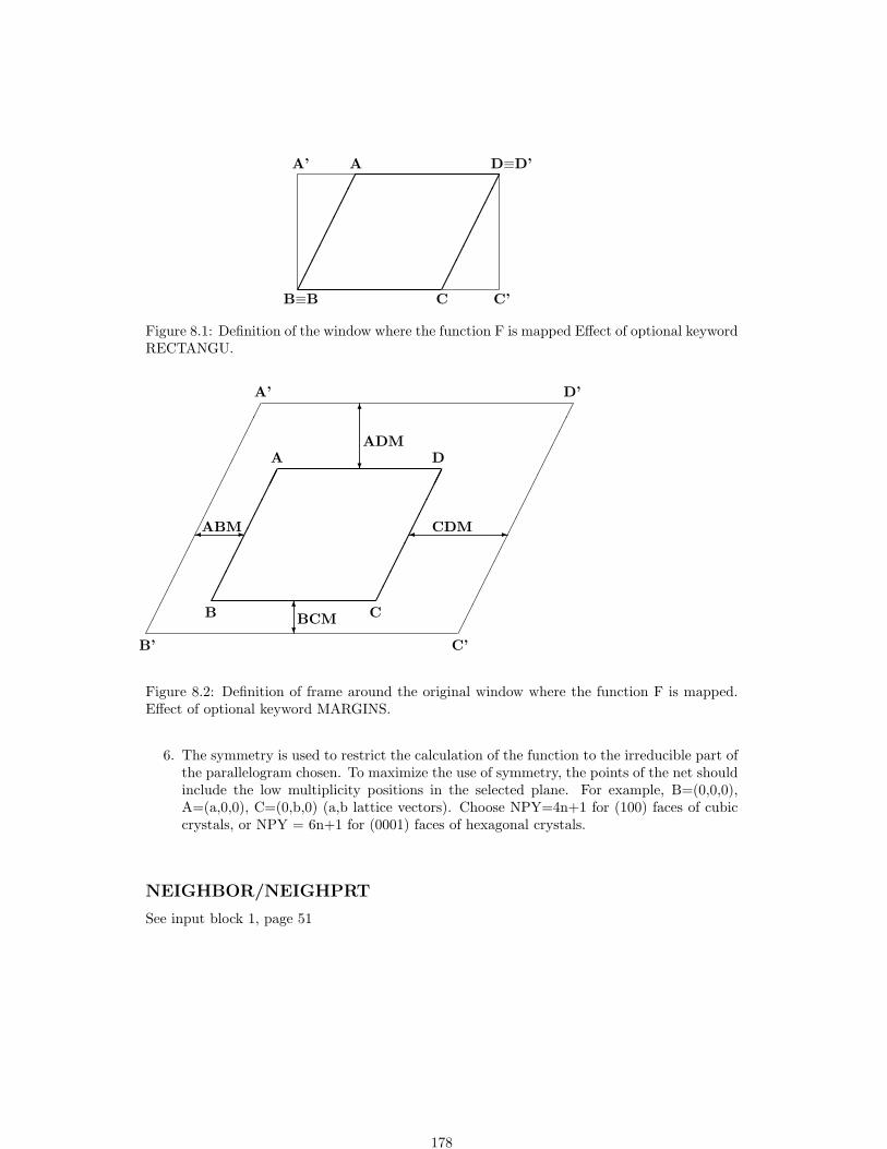
B≡B C C’

A’ A D≡D’

Figure 8.1: Definition of the window where the function F is mapped Effect of optional keywordRECTANGU.

B C

A D

B’ C’

A’ D’

6

?BCM

6

?

ADM

-ABM - CDM

Figure 8.2: Definition of frame around the original window where the function F is mapped.Effect of optional keyword MARGINS.

6. The symmetry is used to restrict the calculation of the function to the irreducible part ofthe parallelogram chosen. To maximize the use of symmetry, the points of the net shouldinclude the low multiplicity positions in the selected plane. For example, B=(0,0,0),A=(a,0,0), C=(0,b,0) (a,b lattice vectors). Choose NPY=4n+1 for (100) faces of cubiccrystals, or NPY = 6n+1 for (0001) faces of hexagonal crystals.

NEIGHBOR/NEIGHPRT


178

NEWK - Hamiltonian eigenvectors

rec variable value meaningif system is periodic, insert II

• ∗ IS Shrinking factor for reciprocal space net (Monkhorst net). The num-ber NKF of k points, where the Fock/KS matrix is diagonalized, isroughly proportional to ISIDIM/MV F where IDIM denotes the pe-riodic dimensionality of the system, and MVF denotes the number ofpoint symmetry operators (see page 23).

ISP Shrinking factor of the secondary reciprocal space net (Gilat net) forthe evaluation of the Fermi energy and density matrix.

if system is periodic and IS=0, insert II• ∗ Shrinking factors of reciprocal lattice vectors

IS1 Shrinking factor along B1IS2 Shrinking factor along B2IS3 Shrinking factor along B3.

• ∗ IFE 0 no Fermi energy calculation is performed;1 Fermi energy is computed, by performing integration on the new k

points net. Total, valence and core density matrices are written onFortran unit 13

NPR number of printing options to switch onif NPR 6= 0 insert prtrec (see page 54) II

The Fock/KS eigenvectors are computed at a number of k points in reciprocal space, definedby the shrinking factor IS, and written unformatted in file fort.10 (in the basis of symmetryadapted Bloch functions) and in file fort.8 (in the basis of AO). Eigenvalues and related infor-mation (coordinates of k points in reciprocal lattice, weights etc) are written in file KIBZ.DATby inserting the keyword CRYAPI OUT (page 160).

1. The Fock/KS matrix in direct space is always the SCF step final one. If the SCF con-vergence was poor, and convergence tools were used, eigenvalues and eigenvectors maybe different from the ones that could be obtained after one more cycle without anyconvergence trick.

2. The shrinking factors IS and ISP (Section 11.7, page 227) can be redefined with respectto the ones used in the SCF process. If this value is smaller than the one used in the scfstep, numerical inaccuracy may occur in the Fourier transform of the Fock/KS matrix,Fg → Fk (Chapter 11, equation 11.5).

3. A Fermi energy calculation must be performed (IFE=1) to run PROF the Comptonprofiles option, PBAN and PDIDE in order to compute the weight associated to eacheigenvalue.

4. Warning NEWK with IFE=1 must be run to obtain the correct Fermi energy and eigen-values spectra when a shift of eigenvalues was requested in SCF (LEVSHIFT, page 92;SPINLOCK, page 101; BETALOCK, 73.A new density matrix is computed. If the convergence of scf was poor, and convergencetools were used (FMIXING, LEVSHIFT, ..), the density matrix obtained from the eigen-vectors computed by NEWK may be different from the matrix that could be calculatedwith one more scf cycle. Properties depending on the density matrix may be different ifcomputed before or after NEWK.

5. if BAND is called after NEWK, and symmetry adapted Bloch functions are used(default option), the information generated by NEWK is destroyed. For instance, tocompute density of states and bands, the sequence must be: BAND - NEWK - DOSS.The sequence NEWK BAND DOSS will give the error message:NEWK MUST BE CALLED BEFORE DOSS

Printing options: 59 (Density matrix - direct lattice); 66 (Hamiltonian eigenvalues); 67 (Hamil-tonian eigenvectors).

179

NOSYMADA


PARAMPRT - - printing of parametrized dimensions


PATO - Density matrix as superposition of atomic densities

rec variable value meaning• ∗ IBN 0 density matrix computed with the same basis set as in the crystal cal-

culation.6= 0 new basis set and/or new electron configuration is given

NPR 6= 0 printing of the density matrix for the first NPR direct lattice vectorsif IBN 6= 0 insert basis set input (page 19) II

1. The PATO option is used for calculating crystal properties, such as charge density(ECHG), structure factors (XFAC) with a periodic density matrix obtained as a su-perposition of atomic solutions (periodic array of non interacting atoms). The reducibledensity matrix is written to file fort.13.

2. The atomic wave function is computed by the atomic program [6], using HF hamiltonian,s, p, d orbitals basis set, properly handling the open shell electronic configuration.

3. If the basis set used for the crystalline calculation (given as input of the integral part)is not suitable for describing a free- atom or free-ion situation, a new basis set can besupplied (see Section 1.2). When this option is used (IBN.NE.0) the basis set of all theatoms with different conventional atomic number has to be provided.

4. The electronic configuration of selected atoms may be modified (CHEMOD in basis setinput). This allows calculation of the density matrix as superposition of atomic densitiesor ionic densities, for the same crystal structure.

5. The wave function data stored in file fort.9 at the end of the SCF cycles are not modified.Only the data stored on the temporary data set (reducible density matrix in fortran unit13 and overlap matrix in fortran unit 3) are modified. The keyword PSCF restores thescf density matrix and all the original information (including geometry and basis set).

6. See also ATOMHF, input block 3, page 72, and CHARGED, input block 2, page 62.

PBAN/PDIBAN - Band(s) projected density matrix

rec variable meaning• ∗ NB number of bands to consider.

NPR printing of the density matrix for the first NPR direct lattice cells.• ∗ N(I),I=1,NB sequence number of the bands summed up for the projected density ma-

trix.

A density matrix projected onto a given range of bands is computed and stored in fortran unit13. The properties will subsequently be computed using such a matrix.For spin polarized systems, two records are written:first record, total density matrix (N=nα + nβ electrons);second record, spin density matrix (Ns=nα - nβ electrons).

To be combined only with ECHG and PPAN. Fock/Kohn-Sham eigenvectors and bandweights must be precomputed by running NEWK and setting IFE=1.

180

PGEOMW - Density matrix from geometrical weights

A density matrix projected onto the range of bands defined in input (see PBAN input instruc-tions) is computed, using the geometrical weights of the k points in the reciprocal lattice. Theproperties will subsequently be computed using such a matrix. All the bands are attributed anoccupation number 1., independently of the position of the Fermi energy. The density matrixdoes not have any physical meaning, but the trick allows analysis of the virtual eigenvectors.For spin polarized systems, two records are written:first record, total density matrix (N=nα + nβ electrons);second record, spin density matrix (Ns=nα - nβ electrons).To be combined only with ECHG and PPAN.Fock/Kohn-Sham eigenvectors and band weights must be computed by running NEWK andsetting IFE=1. Symmetry adaptation of Bloch functions is not allowed, the keyword NOSY-MADA must be inserted before NEWK.

PDIDE - Density matrix energy projected

rec variable meaning• ∗ EMI,EMAX lower and upper energy bound (hartree)

A density matrix projected onto a given energy range is computed and stored in file fort.13.The properties will subsequently be computed using such a matrix. To be combined only withECHG and PPAN. Fock/Kohn-Sham eigenvectors and band weights must be computed byrunning NEWK and setting IFE=1.The charge density maps obtained from the density matrix projected onto a given energy rangegive the STM topography [79] within the Tersoff-Haman approximation [123].

PMP2 - Reads the MP2 correction to the Valence Density Matrix

rec variable value meaning• ∗ IMP2 0 The HF+MP2 Density Matrix is used

1 The MP2 Density Matrix is used

1. The MP2 correction to the Valence Density Matrix, as computed by the CRYSCORprogram, is read from the external unformatted file fort.63, which has to be provided bythe user.

2. The PMP2 keyword must be preceded by NEWK (with IFE=1) since the Fermi energyhas to be computed in order to split the total SCF DM into core and valence densitymatrices. The MP2 correction to the DM is summed to the valence SCF DM.

3. By default the PROPERTIES program adopts the SCF density matrix (DM) but if oneadds the PMP2 keyword in the input file then any property whose corresponding key-word is inserted after PMP2 is computed using the HF+MP2 density matrix (IMP2=0)or the pure MP2 one (IMP2=1), where the former choice is the recommended one andcan be used in order to compute any DM-related quantity, while the latter can be usedjust for plotting electron charge density maps (ECHG keyword).

4. For instance, in order to evaluate the MP2 correction to the X-rays Structure Factors Fhkl,the following sequence of keywords has to be used: NEWK-XFAC-PMP2-XFAC-END; in the output file will be printed the HF Fhkl followed by the HF+MP2 Fhkl.

We report in the following the list of the properties for which the MP2 correction can beevaluated, along with some advices one has to take in mind:

• Directional Compton Profiles (PROF) The ICORE variable must be 1 or 3 and the IVIAvariable must be 1

181

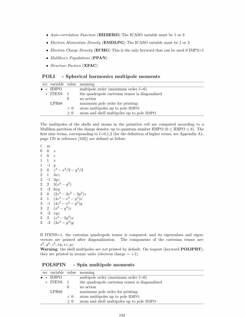
• Auto-correlation Function (BIDIERD) The ICASO variable must be 1 or 3

• Electron Momentum Density (EMDLPG) The ICASO variable must be 1 or 3

• Electron Charge Density (ECHG) This is the only keyword that can be used if IMP2=1

• Mulliken’s Populations (PPAN)

• Structure Factors (XFAC)

POLI - Spherical harmonics multipole moments

rec variable value meaning• ∗ IDIPO multipole order (maximum order `=6)∗ ITENS 1 the quadrupole cartesian tensor is diagonalized

0 no actionLPR68 maximum pole order for printing:

< 0 atom multipoles up to pole IDIPO

≥ 0 atom and shell multipoles up to pole IDIPO

The multipoles of the shells and atoms in the primitive cell are computed according to aMulliken partition of the charge density, up to quantum number IDIPO (0 ≤ IDIPO ≤ 6). Thefirst nine terms, corresponding to `=0,1,2 (for the definition of higher terms, see Appendix A1,page 170 in reference [103]) are defined as follow:

` m0 0 s1 0 z1 1 x1 -1 y2 0 z2 − x2/2− y2/22 1 3xz2 -1 3yz2 2 3(x2 − y2)2 -2 6xy3 0 (2z2 − 3x2 − 3y2)z3 1 (4z2 − x2 − y2)x3 -1 (4z2 − x2 − y2)y3 2 (x2 − y2)z3 -2 xyz3 3 (x2 − 3y2)x3 -3 (3x2 − y2)y

If ITENS=1, the cartesian quadrupole tensor is computed, and its eigenvalues and eigen-vectors are printed after diagonalization. The components of the cartesian tensor are:x2, y2, z2, xy, xz, yzWarning: the shell multipoles are not printed by default. On request (keyword POLIPRT),they are printed in atomic units (electron charge = +1).

POLSPIN - Spin multipole moments

rec variable value meaning• ∗ IDIPO multipole order (maximum order `=6)∗ ITENS 1 the quadrupole cartesian tensor is diagonalized

0 no actionLPR68 maximum pole order for printing:

< 0 atom multipoles up to pole IDIPO

≥ 0 atom and shell multipoles up to pole IDIPO

182

The electron spin density is partitioned in atomic contributions according to the Mullikenscheme, and the spherical harmonic atomic multipoles up to the IDIPO angular quantumnumber are evaluated (see the POLI keyword for definition of the multipoles and references).The Cartesian tensor Tij =

∫xixj ρ

spin(r) dr is computed and diagonalized, and its eigenvaluesand eigenvectors are printed. This option may be useful in the analysis of the size, shape andorientation of localized electron holes.

POT3 - Electrostatic potential on a 3D grid

rec variable meaning• ∗ NP Number of points along the first direction• ∗ ITOL penetration tolerance (suggested value: 5) (see POTM, page 185)

if non-3D systemkeyword to choose the type of grid on the non-periodic direction(s):

SCALE RANGElength scales for non-periodic dimensions boundary for non-periodic dimensions (au)

if 2D system• ∗ ZSCALE • ∗ ZMIN

• ∗ ZMAX

if 1D system• ∗ YSCALE,ZSCALE • ∗ YMIN,ZMIN

• ∗ YMAX,ZMAX

if 0D system• ∗ XSCALE,YSCALE,ZSCALE • ∗ XMIN,YMIN,ZMIN

• ∗ XMAX,YMAX,ZMAX

The electrostatic potential is computed at a regular 3-dimensional grid of points. The gridis defined by the lattice vectors of the primitive unit cell and user defined extents in non-periodic directions. NP is the number of points along the first lattice vector (or XMAX-XMINfor a molecule). Equally spacing is used along the other vectors. Non-periodic extents maybe specified as an explicit range (RANGE) or by scaling the extent defined by the atomiccoordinates (SCALE).

Formatted data are written in fortran unit 31 (function value at the grid points), in the formatrequired by the visualization program DLV.See Appendix D, page 265, for description of the format.

Function data computed at 3D grid points are written according to GAUSSIAN CUBE formatin file POT CUBE.DAT

183

POTC - Electrostatic potential and its derivatives

rec variable meaning• ∗ ICA 0 calculation of potential (V ), its first derivative (E) and second derivatives (E′)

in one or more points1 not implemented2 calculation of V (z), E(z), E′(z) and ρ(z) averaged in the plane at z position

(2D only)3 calculation of V (z), E(z), E′(z) and ρ(z) averaged in the volume between z–ZD

and z+ZD (2D only)NPU n number of points at which these properties are computed

0 these properties are computed at the atomic positions defined by IPA valueIPA 0 calculations are performed at each atomic positions in the cell

1 calculations are performed just for non equivalent atomic positions in the cellif ICA = 0 then

if NPU > 0 insert NPU records II• ∗ X,Y,Z point coordinates (cartesian, bohr)

if NPU < 0 data are read from file POTC.INP IIif ICA = 2 insert II

• ∗ ZM,ZP properties are averaged over NPU planes orthogonal to the z axis from z = ZPto z = ZM by step of (ZP–ZM)/(NPU–1) (bohr)

if ICA = 3 insert II• ∗ ZM,ZP properties are averaged over NPU volumes centered on planes orthogonal to

the z axis, same as ICA = 2ZD half thickness of the volume (bohr)

The exact electrostatic potential V , its derivatives E (electric field) and E′ (electric fieldgradient) are evaluated for molecules (0D), slabs (2D) and crystals (3D). Plane and volumeaveraged properties can be computed for slabs (2D) only. The plane is orthogonal to the zaxis.For ICA = 3, the volume average is performed around a middle plane at z position, from z–ZDto z+ZD, giving a thickness of 2∗ZD.According to Poisson’s law, the charge density ρ(z) is defined as

ρ(z) = − 14π

d2V (z)dz2

=−E′(z)

4πIf an electric field of intensity E0 is present (keyword FIELD, see page 2.1, only for slabs),the total potential Vfield(z) is calculated:

Vfield(z) = V (z)− E0z

where V (z) is the potential of the slab itself and −E0z is the perturbation applied.

• ICA = 0 ; NPU > 0; 2D or 3D systemIt is possible to enter the cartesian coordinates (bohr) of the points where the exactvalue of the properties must be computed. It is useful when applying fitting procedureto obtain formal point charges.

• ICA = 0 ; NPU < 0; 2D or 3D systemcoordinates in bohr are read (free format) from file POTC.INP

record type of data content1 1 integer N, number of points

2..2+N-1 4 real x y z

• ICA 6= 0; NPU 6= 0; 2D or 3D system

The data computed are written in file POTC.DAT. See Appendix D, page 262.

184

POTM - Electrostatic potential maps and electric field

rec variable value meaning• ∗ IDER 0 the electrostatic potential is evaluated

1 the potential and its first derivatives are evaluatedITOL penetration tolerance (suggested value: 5)

insert MAPNET input records (page 177)

1. When IDER=0, the electrostatic potential is calculated at the nodes of a 2-dimensionalnet in a parallelogram-shaped domain defined by the segments AB and BC (see keywordMAPNET, page 177). The electrostatic potential values are written formatted in filefort.25 (see Appendix D, page 259).

2. When IDER 6= 0, the electrostatic potential gradient is computed at the nodes of thesame grid. The x, y and z components are printed in the standard output, and writtenformatted in file fort.25 (see Appendix D, page 259).

3. The electrostatic potential at r is evaluated [114] by partitioning the periodic chargedensity ρ(r) in shell contributions ρh

λ:

ρ(r) =∑

h

∑λ

ρλ(r − h)

(h translation vector).

4. The long range contributions are evaluated through a multipolar expansion of ρλ(r − h)[129]. The short range contributions are calculated exactly.

5. The separation between long and short range is controlled by ITOL: ρλ(r−h) is attributedto the short range (exact) region if

e−αλ(r−sλ−h)2 > 10−ITOL

where: αλ = exponent of the adjoined gaussian of shell λ; sλ = internal coordinates ofshell λ in cell at h.

The difference between the exact and the approximated potential is smaller than 1%when ITOL=5 (input datum to POTM), and IDIPO=4 (input datum to POLI), andsmaller than 0.01% when ITOL=15 and IDIPO=6 [114, 129].

6. The multipoles of shell charges are computed if POLI option was not run before POTM.

PPAN/MULPOPAN - Mulliken Population Analysis




185

PROF - Compton Profiles

rec variable value meaning• ∗ ICORE 1 core plus valence calculation.

2 core only calculation.3 valence only calculation.

IVIA 0 valence contribution is computed by numerical integration.1 valence contribution is computed analytically.

NPR number of printing options to switch on.IPLO 0 CP related data are not stored on disk

1 formatted CP data stored in file fort.25 (Appendix D, page 261)2 formatted CP data stored in Fortran unit 24 (Appendix D, page 261)

if NPR 6= 0 insert prtrec (see page 54) II• A2 CP calculation of Compton profiles (J(q)) along selected directions (eq.

11.27).• ∗ ND number of directions (≤ 6).

REST maximum value of q for J(q) calculation (bohr−1).RINT internal sphere radius (bohr−1).IRAP shrinking factor ratio.

• ∗ (KD(J,N), J=1,3),N=1,ND

directions in oblique coordinates; see note 9

• ∗ STPJ interpolation step (in interpolated Compton profiles calculation).• A4 DIFF CP difference between all computed directional CPs.

• A2 BR auto-correlation function B(r) calculation (eq. 11.30).• ∗ RMAX maximum r value (bohr) at which B(r) is computed

STBR step in computation of B(r).• A4 CONV convolution of the data previously computed (CP, DIFF, BR) (eq.

11.29)• ∗ FWHM convolution parameter (a.u.) full width half maximum;

σ =√

(FWHM)2/(8 · 2log2).• A4 ENDP End of input records for CP data

The keyword PROF starts the calculation of Compton profiles (J(q)) along selected directions(eq. 11.27). The specific keywords DIFF BR CONV allow the calculation of the relatedquantities. The card with the keyword ENDP ends the Compton profiles input section.

1. The input of the options must be given in the order in which they appear in the abovedescription. To enter this property, the CP option must always be selected after PROF,while the others are optional.

2. Core and valence contributions are computed by using different algorithms. Core con-tribution to CP’s is always computed analytically via the Pg matrix (direct lattice sum-mation, equation 11.25); the valence contribution is computed numerically (IVIA=0) byintegrating the EMD (equation 11.23). Valence contribution can be evaluated analyti-cally, setting IVIA=1.

3. The numerical integration is extended to a sphere (radius RINT) where EMD is sampledat the points of a commensurate net characterized by a shrinking factor IS (in the IBZ)and at all the points (with modulus less then RINT) obtained from these by applyingreciprocal lattice translations.

It is possible to define a second sphere (with radius REST); in the volume betweenthe two spheres a second net is employed with shrinking factor IS1 greater then IS.IRAP=IS1/IS is given in INPUT card 2; a reasonable value is IRAP=2. The outercontribution is supposed to be the same for different CP’s, and is obtained by integratingthe average EMD.

186

4. If ICORE 6= 2 (valence electron CP’s are required) the NEWK option, with IFE=1,must be run before the PROF option, in order to generate the eigenvectors required forthe EMD calculation, as well as the weights associated with each k point.

5. If ICORE 6= 2 and IVIA = 0 the CPs are evaluated at points resulting from the ISpartition of the reciprocal lattice translators. The interpolation is performed at STPJintervals (STPJ is given in input).

If ICORE = 2 or IVIA = 1 the CPs are, in any case, evaluated at points resulting fromSTPJ intervals.

IVIA=0 (numerical integration) produces much more accurate results;

IVIA=1 (analytical integration) is to be used only for molecular calculations or for nonconducting polymers.

6. Total CP’s are always obtained by summing core and valence contributions.

7. Reasonable values of the integration parameters depend on the system under investi-gation. The normalization integral of the CP’s is a good check of the accuracy of thecalculation. For instance, in the case of the valence electron of beryllium (test 9), goodvalues of RINT and IS are 10. a.u. and 4 respectively. In the case of silicon (test 10),good values of the same variables are 8. a.u. and 8 respectively. Much greater RINTvalues are required in order to include all the core electrons (70. a.u. in the case ofsilicon, and 25. a.u. in the case of beryllium).

8. BR (auto-correlation function or reciprocal space form factor) should be calculated onlyfor valence electrons. All electron BR are reliable when the normalization integral, afterthe analytical integration for core electrons contribution, is equal to the number of coreelectrons.

9. The oblique coordinates directions given in input refer to the conventional cell, not tothe primitive cell for 3D systems.

Example: in a FCC system the input directions refer to the orthogonal unit cell frame(sides of the cube) not to the primitive non-orthogonal unit cell frame.

Printing options: 116 (Compton profiles before interpolation); 117 (average EMD before inter-polation); 118 (printing of core, valence etc. contribution). The LPRINT(118) option shouldbe used only if ICORE=1, that is, if core plus valence calculation are chosen.

PSCF - Restore SCF density matrix

The wave function data computed at the last SCF cycle are restored in common areas andfortran units 3 (overlap matrix), 11 (Fock/KS matrix), 13 (density matrix). The basis setdefined in input block 2 is restored. Any modification in the default settings introduced inproperties is overwritten. No input data required.

RAYCOV - covalent radii modification


ROTREF - Rotation of eigenvectors and density matrix

This option permits the rotation of the cartesian reference frame before the calculation of theproperties.It is useful, for example, in the population analysis or in the AO projected density of states ofsystems containing transition metal atoms with partial d occupation.Consider for example a d7 occupation as in CoF2, where the main axis of the (slightly distorted)CoF6 octahedron in the rutile structure makes a 450 angle with the x axis, and lies in the xyplane, so that the three empty β states are a combination of the 5 d orbitals. Re-orienting theoctahedron permits to assign integer β occupations to dxz and dyz.

187

Input for the rotation as for EIGSHROT (page 82)





STOP


SYMADAPT


XFAC - X-ray structure factors

rec variable value meaning• ∗ ISS > 0 number of reflections whose theoretical structure factors are calculated.

< 0 a set of non-equivalent reflections with indices h,k,l < |ISS| is gener-ated

if ISS > 0 insert ISS records II• ∗ H,K,L Miller indices of the reflection (conventional cell) .

The Fourier transform of the ground state charge density of a crystalline system provides thestatic structure factors of the crystal, which can be determined experimentally, after takinginto account a number of corrective terms, in particular those related to thermal and zero pointmotion of nuclei:

Fk =∫ρ(r) eik·rdr

where k ≡ h b1 + k b2 + l b3. The Miller indices refer to the conventional cell. The structurefactors are integrated over the primitive cell volume.

188

8.3 Spontaneous polarization and piezoelectricity

Y. Noel, September 2002 - not fully updated to CRYSTAL09

PIEZOBP - Piezoelectricity (Berry phase approach)

The calculation the piezoelectric constants of a system, can be decompose in few steps. Apreliminary run must be performed for the undistorted system (λ = 0) with the keywordPOLARI. Then, for a first distorted system (λ = 1), a second preliminary run (with thekeyword POLARI) must be performed, followed by third run with the keyword PIEZOBPthat calculates a approximated value of the piezoelectric constants. The evaluation of the slopedϕα

dεjkis computed with a single point. For more accuracy, other runs must be done for other

distortions (one run with the keyword POLARI of the new system, followed by a second runwith the keyword PIEZOBP with the undistorted and the new distorted systems). Then themean value of the obtained piezoelectric constants must be performed.

1. First run: preliminary calculation related to system λ = 0 (undistorted)

Program Keyword commentscrystal see deck 1 for input blocks 1 and 1bproperties NEWK additional keywords allowed

POLARI see abovesave Fortran unit 27 as undistord.f27

2. Second run: preliminary calculation related to system λ = 1 (distorted)

Program Keyword commentscrystal see deck 1 for input blocks 1 and 1bproperties NEWK same input as in first run

POLARIsave Fortran unit 27 as distord1.f27

3. Third run: merging of previous data.

copy undistord.f27 to Fortran unit 28copy distord1.f27 to fortran unit 29Program Keyword commentsproperties PIEZOBP

4. Refine the computed value

Repeat 2. and 3. for several distortions.Then compute the mean value of the piezoelectric constants obtained in each case.

PIEZOWF - Piezoelectricity (localized CO approach)

The calculation the piezoelectric constants of a system, can be decompose in few steps. Apreliminary run must be performed for the undistorted system (λ = 0) with the keywordLOCALWF. Then, for a first distorted system (λ = 1), a second preliminary run (with thekeyword LOCALWF) must be performed, followed by third run with the keyword PIEZOWFthat calculates a approximated value of the piezoelectric constants. The evaluation of the slopedϕα

dεjkis computed with a single point. For more accuracy, other runs must be done for other

distortions (one run with the keyword LOCALWF of the new system, followed by a secondrun with the keyword PIEZOWF with the undistorted and the new distorted systems). Thenthe mean value of the obtained piezoelectric constants must be performed.

189

1. First run: preliminary calculation related to system λ = 0 (undistorted)


LOCALWF see abovesave Fortran unit 37 as undistord.f37

2. Second run: preliminary calculation related to system λ = 1 (distorted)


LOCALWFsave Fortran unit 37 as distord1.f37


copy undistord.f37 to Fortran unit 38copy distord1.f37 to Fortran unit 39Program Keyword commentsproperties PIEZOWF

4. Refine the computed value

Repeat 2. and 3. for several distortions.Then compute the mean value of the piezoelectric constants obtained in each case.

POLARI - Spontaneous polarization (steps 1 and 2)

PHASE - Spontaneous polarization (step 3)

The ferroelectric phases of a ferroelectric material exhibit two possible enantiomorphic noncentrosymmetric structures, which can be labelled by the geometric parameters λ=+1 andλ=−1. An external electric field can force the system to change from one structure to theother, passing through a small energy maximum. The centrosymmetric unstable structurewhich sits in the middle of the λ=+1 and λ=−1 structures can be labelled by the geometricparameters λ=0.The spontaneous polarization in ferroelectric materials is then evaluated through the Berryphase approach [107, 30] as the polarization difference between one of the two enantiomorphicstructures (λ=+1 or λ=−1) and the intermediate geometric structure (λ=0).The fortran unit 70 is defined as direct access:

OPEN(UNIT=IO70,ACCESS=’DIRECT’,RECL=LREC)

Three subsequent runs are required.

1. First run: preliminary calculation related to λ=0 structure

Program Keyword commentscrystal see deckproperties NEWK see page 179

POLARI no input data requiredmove fortran unit 27 to zero.f27

2. Second run: preliminary calculation related to λ=+1 (or λ=−1) structure

190

Program Keyword commentscrystal see deck 2properties NEWK same input as in first run

POLARI no input data requiredmove fortran unit 27 to one.f27

3. Third run: merging of previous data

fortran unit 9 of previous calculation must be presentcopy zero.f27 to fortran unit 28copy one.f27 to fortran unit 29

Program Keyword commentsproperties PHASE no input data required

END terminate processing of polari keywords

Deck 1Potassium niobate - KNbO3

CRYSTAL 3D system0 0 0 IFLAG IFHR IFSO123 space group, P4/mmm3.997 4.063 lattice parameters4 4 non equivalent atoms (5 atoms in the primitive cell)19 0.5 0.5 0.5 Z=19, Potassium; x, y, z (multiplicity 1)8 0.0 0.0 0.5 Z=8, Oxygen I; x, y, z (multiplicity 1)8 0.5 0.0 0.0 Z=8, Oxygen II; x, y, z (multiplicity 2)41 0.0 0.0 0.0 Z=41, Niobium; x, y, z (multiplicity 1)END end of geometry input records

Deck 2Potassium niobate - KNbO3

CRYSTAL 3D system0 0 0 IFLAG IFHR IFSO123 space group, P4/mmm3.997 4.063 lattice parameters4 4 non equivalent atoms (5 atoms in the primitive cell)19 0.5 0.5 0.5 Z=19, Potassium; x, y, z (multiplicity 1)8 0.0 0.0 0.5 Z=8, Oxygen I; x, y, z (multiplicity 1)8 0.5 0.0 0.0 Z=8, Oxygen II; x, y, z (multiplicity 2)41 0.0 0.0 0.0 Z=41, Niobium; x, y, z (multiplicity 1)FRACTION fractional coordinatesATOMDISP displacement of atoms4 four atoms to be displaced1 0.0 0.0 -0.023 displacement of atom no. 1 (Potassium)2 0.0 0.0 -0.042 displacement of atom no. 2 (Oxygen II)3 0.0 0.0 -0.042 displacement of atom no. 3 (Oxygen II)4 0.0 0.0 -0.040 displacement of atom no. 4 (Oxygen I)END end of geometry input records

1. The unit-cell has to contain an even number of electrons.

2. Cell parameters have to be the same for whatever value of the geometric parameterλ. The difference between the λ=+1, λ=0, and λ=−1 structures is only in the atomicpositions.

3. Numerical accuracy and computational parameters in input block 3 (such as TOLIN-TEG, POLEORDR, etc.) should be the same for the first and the second run.

4. See page 179 for the NEWK input, which has to be the same for the first and the secondrun. The shrinking factor IS should be at least equal to 4. Fermi energy calculation isnot necessary, then set IFE=0.

191

5. Data evaluated with the keyword POLARI in the first two runs do not have any physicalmeaning if considered independently. Only the output produced choosing the keywordPHASE in the third run is significant.

6. When the λ=−1 geometric structure is chosen in the second run, the spontaneous polar-ization vector obtained at the end will have the same modulus and direction but oppositeversus with respect to the vector obtained by choosing the λ=+1 structure.

7. The spontaneous polarization is obtained through the Berry phase approach. Since aphase is defined only in the interval −π to +π, each component of the spontaneouspolarization vector is defined to within an integer number (positive or negative) of thecorrespondent component of the ”quantum of polarization” vector, which is automaticallyshown in the output of the third run.Usually there is not need to take into account the quantum of polarization vector, unlessthe ferroelectric material shows a large value of the spontaneous polarization.In case of doubt whether the quantum of polarization vector has to be considered ornot, it is possible to evaluate the spontaneous polarization by setting in the second run ageometric structure corresponding to an intermediate geometric parameter, e.g. λ=0.25,and then to extrapolate linearly the result to the λ=1 structure.

SPOLBP - Spontaneous polarization (Berry phase approach)

To calculate the spontaneous polarization, a preliminary with the keyword POLARI run is neededfor each of the two systems λ = 1 and λ = 0. Then a third run with the keyword SPOLBPgives the difference of polarization between both systems.

1. First run: preliminary calculation related to system λ = 0


POLARI see abovesave Fortran unit 27 as sys0.f27

2. Second run: preliminary calculation related to system λ = 1


POLARIsave Fortran unit 27 as sys1.f27


copy sys0.f27 to Fortran unit 28copy sys1.f27 to Fortran unit 29Program Keyword commentsproperties SPOLBP

192

SPOLWF - The spontaneous polarization (localized CO approach)

To calculate the spontaneous polarization, two preliminary runs with the keyword LOCALIis needed for each of the two systems λ = 1 and λ = 0. Then a third run with the keywordSPOLBP computes the difference of polarization between both systems.

1. First run: preliminary calculation related to system λ = 0


LOCALI see abovesave Fortran unit 37 as sys0.f23

2. Second run: preliminary calculation related to system λ = 1


LOCALIsave Fortran unit 37 as sys1.f37


copy sys0.f37 to Fortran unit 38copy sys1.f37 to Fortran unit 39Program Keyword commentsproperties SPOLWF

193

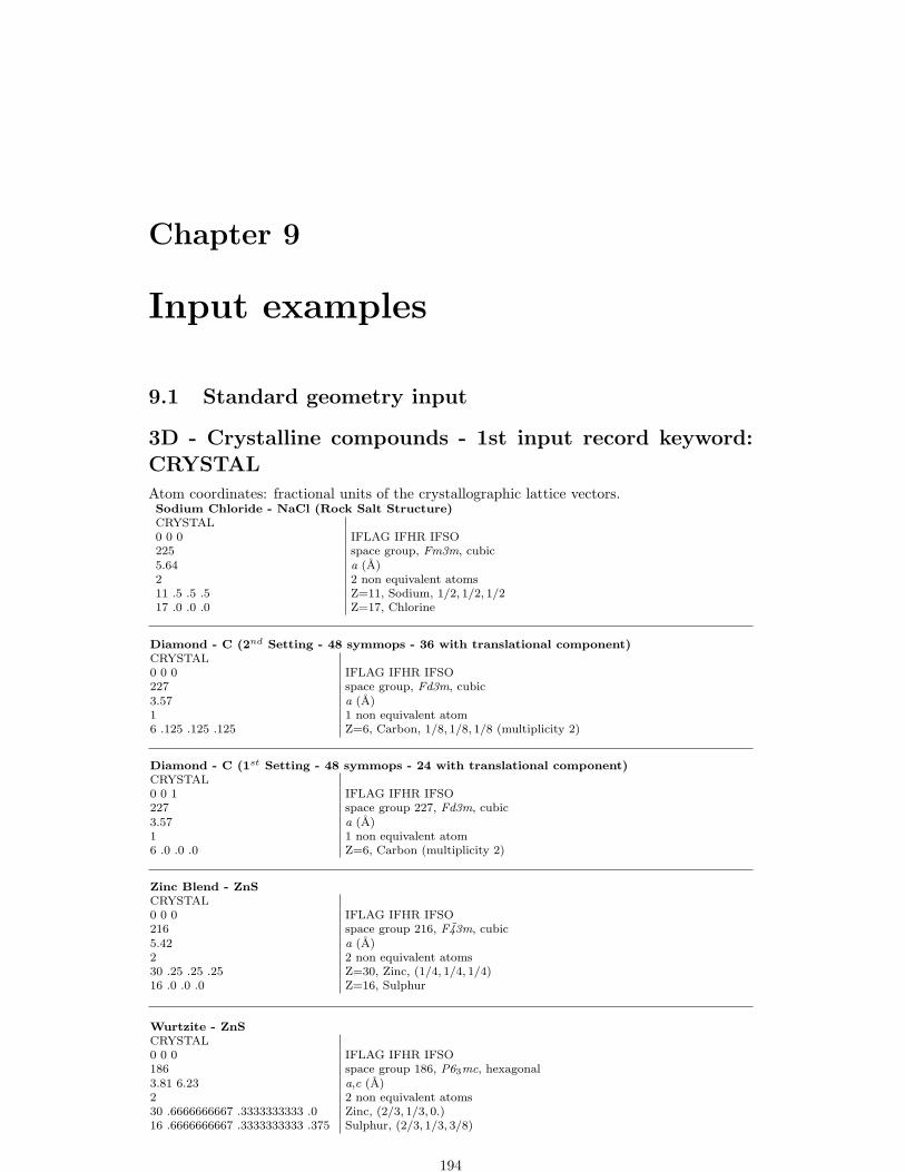
Chapter 9

Input examples

9.1 Standard geometry input

3D - Crystalline compounds - 1st input record keyword:CRYSTAL

Atom coordinates: fractional units of the crystallographic lattice vectors.Sodium Chloride - NaCl (Rock Salt Structure)CRYSTAL0 0 0 IFLAG IFHR IFSO225 space group, Fm3m, cubic5.64 a (A)2 2 non equivalent atoms11 .5 .5 .5 Z=11, Sodium, 1/2, 1/2, 1/217 .0 .0 .0 Z=17, Chlorine

Diamond - C (2nd Setting - 48 symmops - 36 with translational component)CRYSTAL0 0 0 IFLAG IFHR IFSO227 space group, Fd3m, cubic3.57 a (A)1 1 non equivalent atom6 .125 .125 .125 Z=6, Carbon, 1/8, 1/8, 1/8 (multiplicity 2)

Diamond - C (1st Setting - 48 symmops - 24 with translational component)CRYSTAL0 0 1 IFLAG IFHR IFSO227 space group 227, Fd3m, cubic3.57 a (A)1 1 non equivalent atom6 .0 .0 .0 Z=6, Carbon (multiplicity 2)

Zinc Blend - ZnSCRYSTAL0 0 0 IFLAG IFHR IFSO216 space group 216, F43m, cubic5.42 a (A)2 2 non equivalent atoms30 .25 .25 .25 Z=30, Zinc, (1/4, 1/4, 1/4)16 .0 .0 .0 Z=16, Sulphur

Wurtzite - ZnSCRYSTAL0 0 0 IFLAG IFHR IFSO186 space group 186, P63mc, hexagonal3.81 6.23 a,c (A)2 2 non equivalent atoms30 .6666666667 .3333333333 .0 Zinc, (2/3, 1/3, 0.)16 .6666666667 .3333333333 .375 Sulphur, (2/3, 1/3, 3/8)

194

Cuprite - Cu2OCRYSTAL0 0 0 IFLAG IFHR IFSO208 space group 208, P4232, cubic4.27 a (A)2 2 non equivalent atoms8 .0 .0 .0 Z=8, Oxygen29 .25 .25 .25 Z=29, Copper (1/4, 1/4, 1/4)

Aragonite - CaCO3

CRYSTAL1 0 0 IFLAG (1, SPGR symbol) IFHR IFSOP M C N space group Pmcn, orthorhombic4.9616 7.9705 5.7394 a,b,c (A)4 4 non equivalent atoms20 .25 .4151 .2103 Z=20, Calcium6 .25 .7627 .085 Z=6, Carbon8 .25 .9231 .0952 Z=8, Oxygen8 .4729 .6801 .087 Z=8, Oxygen

Fluorite - CaF2

CRYSTAL0 0 0 IFLAG IFHR IFSO225 space group 225, Fm3m, cubic5.46 a (A)2 2 non equivalent atoms9 .25 .25 .25 Fluorine20 .0 .0 .0 Calcium

Cesium chloride - CsClCRYSTAL0 0 0 IFLAG IFHR IFSO221 space group 221, Pm3m, cubic4.12 a (A)2 2 non equivalent atoms55 .5 .5 .5 Cesium17 .0 .0 .0 Chlorine

Rutile - TiO2

CRYSTAL0 0 0 IFLAG IFHR IFSO136 space group 136, P42/mnm, tetragonal4.59 2.96 a, c (A)2 2 non equivalent atoms22 .0 .0 .0 Titanium8 .305 .305 .0 Oxygen

Graphite - C (Hexagonal)CRYSTAL0 0 0 IFLAG IFHR IFSO194 space group 194, P63/mmc, hexagonal2.46 6.70 a,c (A)2 2 non equivalent atoms6 .0 .0 .25 Carbon, 0, 0, 1/46 .33333333333 .66666666667 .25 Carbon, 1/3, 2/3, 1/4

Pyrite - FeS2

CRYSTAL0 0 0 IFLAG IFHR IFSO205 space group 205, Pa3, cubic5.40 a (A)2 2 non equivalent atoms26 .0 .0 .0 Iron16 .386 .386 .386 Sulphur

195

Calcite - CaCO3

CRYSTAL0 1 0 IFLAG IFHR (=1, rhombohedral representation) IFSO167 space group 167, R3c, hexagonal6.36 46.833 a (A), α

3 3 non equivalent atoms20 .0 .0 .0 Calcium6 .25 .25 .25 Carbon8 .007 .493 .25 Oxygen

Corundum - Al2O3 (hexagonal representation)CRYSTAL0 0 0 IFLAG IFHR IFSO167 space group 167, R3c, hexagonal4.7602 12.9933 a,c (A)2 2 non equivalent atoms13 0. 0. 0.35216 Aluminium8 0.30621 0. 0.25 Oxygen

Corundum - Al2O3 (rhombohedral representation)CRYSTAL0 1 0 IFLAG IFHR (=1, rhombohedral cell) IFSO167 space group 167, R3c, hexagonal5.12948 55.29155 a (A), α

2 2 non equivalent atoms13 0.35216 0.35216 0.35216 Aluminium8 0.94376 0.25 0.55621 Oxygen

Zirconia - ZrO2 - monoclinic structureCRYSTAL0 0 1 IFLAG IFHR IFSO (=1, standard shift of origin)14 space group 14, P21/c, monoclinic5.03177 5.03177 5.258 90.0 a,b,c (A), β

3 3 non equivalent atoms240 0.2500 0.0000 0.25000 Zirconium, Pseudopotential (Z’ > 200)208 0.0000 0.2500 0.07600 Oxygen, Pseudopotential208 -0.500 -0.250 0.07600 Oxygen, Pseudopotential

Zirconia - ZrO2 - tetragonal structureCRYSTAL0 0 1 IFLAG IFHR IFSO (=1, standard shift of origin)137 space group 137, P42/nmc, tetragonal3.558 5.258 a,c (A)3 3 non equivalent atoms240 0.0 0.0 0.0 Zirconium, Pseudopotential (Z’ > 200)208 0.0 -0.5 0.174 Oxygen, Pseudopotential208 0.5 0.0 0.326 Oxygen, Pseudopotential

Zirconia - ZrO2 - cubic structureCRYSTAL0 0 1 IFLAG IFHR IFSO (=1, standard shift of origin)225 space group 225, Fm3m, cubic5.10 a (A)3 3 non equivalent atoms240 0.00 0.00 0.00 Z=40 Zirconium, Pseudopotential (Z’ > 200)208 0.25 0.25 0.25 Oxygen, Pseudopotential208 -0.25 -0.25 -0.25 Oxygen, Pseudopotential

196

SiO2, ChabaziteCRYSTAL0 1 0 IFLAG IFHR (=1,rhombohedral representation) IFSO166 space group 166 R3m, hexagonal9.42 94.47 a (A), β

5 5 non equivalent atoms (36 atoms in the primitive cell)14 .1045 .334 .8755 Silicon (multiplicity 12)8 .262 -.262 .0 Oxygen (multiplicity 6)8 .1580 -.1580 .5000 Oxygen (multiplicity 6)8 .2520 .2520 .8970 Oxygen (multiplicity 6)8 .0250 .0250 .3210 Oxygen (multiplicity 6)

SiO2, Siliceous FaujasiteCRYSTAL0 0 0 IFLAG IFHR IFSO227 space group 227, Fd3m, cubic21.53 a (A)5 5 non equivalent atoms (144 atoms in the primitive cell)14 .1265 -.0536 .0370 Silicon (multiplicity 48)8 .1059 -.1059 .0 Oxygen (multiplicity 24)8 -.0023 -.0023 .1410 Oxygen (multiplicity 24)8 .1746 .1746 -.0378 Oxygen (multiplicity 24)8 .1785 .1785 .3222 Oxygen (multiplicity 24)

SiO2, Siliceous EdingtoniteCRYSTAL0 0 0 IFLAG IFHR IFSO115 space group 115, P4m2, tetragonal6.955 6.474 a, c (A)5 5 non equivalent atoms (15 atoms in the primitive cell)14 .0 .0 .5000 Silicon (multiplicity 1)14 .0 .2697 .1200 Silicon (multiplicity 4)8 .0 .189 .3543 Oxygen (multiplicity 4)8 .50000 .0 .8779 Oxygen (multiplicity 2)8 .189 .189 .0 Oxygen (multiplicity 4)

SiO2, Siliceous SodaliteCRYSTAL0 0 0 IFLAG IFHR IFSO218 space group 218, P43n, cubic8.950675 a (A)3 3 non equivalent atoms (36 atoms in the primitive cell)14 .25000 .50000 .0 Silicon (multiplicity 6)14 .25000 .0 .50000 Silicon (multiplicity 6)8 .14687 .14687 .50000 Oxygen (multiplicity 24)

197

2D - Slabs (surfaces) - 1st input record keyword: SLAB

A 2D structure can either be created by entering directly the 2D cell parameters andirreducible atoms coordinates to obtain a slab of given thickness (keyword SLAB in the firstrecord of the geometry input), or it can be derived from the 3D structure through the keywordSLABCUT (page 55), entered in the geometry editing section of 3D structure input. In thatcase the layer group is automatically identified by the program. The input tests 4-24, 5-25,6-26 and 7-27 show the two different ways to obtain the same 2D structure.Atom coordinates: z in Angstrom, x, y in fractional units of the crystallographic cell translationvectors.

Test05 - graphite 2D (see test 25)

SLAB77 layer group (hexagonal)2.47 lattice vector length (A)1 1 non equivalent atom6 -0.33333333333 0.33333333333 0. Z=6; Carbon; x,y,z

Beryllium - 3 layers slabSLAB78 layer group (hexagonal)2.29 lattice vector length (A)2 2 non equivalent atoms4 0.333333333333 0.666666666667 0. Z=4, Beryllium; 1/3, 2/3, z4 0.666666666667 0.333333333333 1.795 Z=4, Beryllium; 2/3, 1/3,z

Test06 - beryllium - 4 layers slab (see test 26)SLAB72 layer group (hexagonal)2.29 lattice vector length (A)2 2 non equivalent atoms4 0.333333333333 0.666666666667 0.897499 Z=4, Beryllium;x,y,z4 0.666666666667 0.333333333333 2.692499 Z=4, Beryllium;x,y,z

Test04 - Corundum 001 (0001) 2 layers slab (see test 24)SLAB66 layer group (hexagonal)4.7602 lattice vector length (A)3 3 non equivalent atoms13 0. 0. 1.9209 Z=13, Aluminum; x,y,z8 0.333333333 -0.027093 1.0828 Z=8, Oxygen; x,y,z13 -0.333333333 0.333333333 0.2446 Z=13, Aluminum; x,y,z

Test07 - Corundum 110 (1010) slab (see test 27)SLAB7 layer group (Oblique)5.129482 6.997933 95.8395 a,b (A) α (degrees)6 6 non equivalent atoms8 -0.25 0.5 2.1124 Z=8, Oxygen; x,y,z8 0.403120 0.153120 1.9189 Z=8, Oxygen; x,y,z8 0.096880 0.346880 0.4612 Z=8, Oxygen; x,y,z8 -0.25 0.00 0.2677 Z=8, Oxygen; x,y,z13 0.454320 0.397840 1.19 Z=13, Aluminum; x,y,z13 0.045680 0.102160 1.19 Z=13, Aluminum; x,y,z

MgO (110) 2 layers slabSLAB40 layer group4.21 2.97692 lattice vectors length (A)2 2 non equivalent atoms12 0.25 0.25 0.74423 Z=12, Magnesium; x,y,z8 0.75 0.25 0.74423 Z=8, Oxygen; x,y,z

198

MgO (110) 3 layers slabSLAB374.21 2.97692 lattice vectors length (A)4 4 non equivalent atoms12 0. 0. 1.48846 Z=12, Magnesium; x,y,z8 0.5 0. 1.48846 Z=8, Oxygen; x,y,z12 0.5 0.5 0. Z=12, Magnesium; x,y,z8 0. 0.5 0. Z=8, Oxygen; x,y,z

CO on MgO (001) two layers slab - one-side adsorptionSLAB55

2.97692 lattice vector length [4.21/√

2] (A)6 6 non equivalent atoms108 0. 0. 4.5625 Z=8, Oxygen; x,y,z6 0. 0. 3.4125 Z=6, Carbon; x,y,z12 0. 0. 1.0525 Z=12, Magnesium; x,y,z8 0.5 0.5 1.0525 Z=8, Oxygen; x,y,z12 0. 0. -1.0525 Z=12, Magnesium; x,y,z8 0.5 0.5 -1.0525 Z=8, Oxygen; x,y,z

Two different conventional atomic numbers (8 and 108) are attributed to the Oxygen in CO and to the Oxygenin MgO. Two different basis sets will be associated to the two type of atoms (see Basis Set input, page 19, andtest 36).

CO on MgO (001) two layers slab - two-side adsorptionSLAB642.97692 lattice vector length (A)4 4 non equivalent atoms108 0.25 0.25 4.5625 Z=8, Oxygen; x,y,z6 0.25 0.25 3.4125 Z=6, Carbon; x,y,z12 0.25 0.25 1.0525 Z=12, Magnesium; x,y,z8 0.75 0.75 1.0525 Z=8, Oxygen; x,y,z

Two different conventional atomic numbers (8 and 108) are attributed to the Oxygen in CO and to the Oxygenin MgO.

Diamond slab parallel to (100) face - nine layers slabSLAB592.52437 lattice vector length (A)5 5 non equivalent atoms6 0. 0. 0. Z=6, Carbon; x,y,z6 0.5 0. 0.8925 Z=6, Carbon; x,y,z6 0.5 0.5 1.785 Z=6, Carbon; x,y,z6 0. 0.5 2.6775 Z=6, Carbon; x,y,z6 0. 0. 3.57 Z=6, Carbon; x,y,z

Diamond slab parallel to (100) face - ten layers slabSLAB39 layer group2.52437 2.52437 lattice vectors length (A)5 5 non equivalent atoms6 0.25 0. 0.44625 Z=6, Carbon; x,y,z6 0.25 0.5 1.33875 Z=6, Carbon; x,y,z6 0.75 0.5 2.23125 Z=6, Carbon; x,y,z6 0.75 0 3.12375 Z=6, Carbon; x,y,z6 0.25 0. 4.01625 Z=6, Carbon; x,y,z

199

1D - Polymers - 1st input record keyword: POLYMER

Atom coordinates: y,z in Angstrom, x in fractional units of the crystallographic cell translationvector.

Test03 - (SN)x polymer

POLYMER4 rod group4.431 lattice vector length (A)2 2 non equivalent atoms16 0.0 -0.844969 0.0 Z=16, Sulphur; x, y, z7 0.141600540 0.667077 -0.00093 Z=7, Nitrogen; x, y, z

Water polymer

POLYMER14.965635 lattice vector length (A)6 6 non equivalent atoms8 0. 0. 0. Z=8, Oxygen; x, y, z1 0.032558 0.836088 -0.400375 Z=1, Hydrogen; x, y, z1 0.168195 -0.461051 0. Z=1, Hydrogen; x, y, z8 0.5 -1.370589 0. Z=8, Oxygen; x, y, z1 0.532558 -2.206677 0.400375 Z=1, Hydrogen; x, y, z1 0.668195 -0.909537 0. Z=1, Hydrogen; x, y, z

Formamide chain - test40 DFT

POLYMER4 rod group8.774 lattice vector length (A)6 6 non equivalent atoms8 -7.548E-2 5.302E-3 0.7665 Z=8, Oxygen; x, y, z7 0.1590 -0.8838 0.3073 Z=7, Nitrogen; x, y, z6 5.627E-2 7.051E-2 0.2558 Z=6, Oxygen; x, y, z1 0.2677 -0.6952 -9.1548E-2 Z=1, Hydrogen; x, y, z1 0.1310 -1.8019 0.7544 Z=1, Hydrogen; x, y, z1 9.244E-2 0.9973 -0.2795 Z=1, Hydrogen; x, y, z

200

0D - Molecules - 1st input record keyword: MOLECULE

Atom coordinates: x,y,z in Angstrom.Test00 - CO molecule

MOLECULE1 point group2 2 non equivalent atoms6 0. 0. 0. Z=6, Carbon; x, y, z8 0.8 0.5 0.4 Z=8, Oxygen; x, y, z

Test01 - CH4 Methane molecule

MOLECULE44 point group2 2 non equivalent atoms6 0. 0. 0. Z=6, Carbon; x, y, z1 0.629 0.629 0.629 Z=1, Hydrogen; x, y, z

Test02 - CO(NH2)2 Urea molecule

MOLECULE15 point group5 5 non equivalent atoms6 0. 0. 0. Z=6, Carbon; x, y, z8 0. 0. 1.261401 Z=8, Oxygen; x, y, z7 0. 1.14824666034 -0.69979 Z=7, Nitrogen; x, y, z1 0. 2.0265496501 -0.202817 Z=1, Hydrogen; x, y, z1 0. 1.13408048308 -1.704975 Z=1, Hydrogen; x, y, z

9.2 Basis set input

Optimized basis sets for periodic systems used in published papers are available on WWW:


All electron Basis sets for Silicon atom

STO-3G14 3 Z=14, Silicon; 3 shells1 0 3 2. 0. Pople BS; s shell; 3G; CHE=2; standard scale factor1 1 3 8. 0. Pople BS; sp shell; 3G; CHE=8; standard scale factor1 1 3 4. 0. Pople BS; sp shell; 3G; CHE=4; standard scale factor

6-21G14 4 Z=14, Silicon; 4 shells2 0 6 2. 1. Pople 6-21 BS; s shell; 6G; CHE=2; scale factor 1 (core AO).2 1 6 8. 1. Pople 6-21 BS; sp shell; 6G; CHE=8; scale factor 1 (core AOs).2 1 2 4. 1. Pople 6-21 BS; sp shell; 2G; CHE=4; scale factor 1 (inner valence).2 1 1 0. 1. Pople 6-21 BS; sp shell; 1G; CHE=0; scale factor 1 (outer valence).

NB. The 4th shell has electron charge 0. The basis functions of that shell are included in the basis set tocompute the atomic wave functions, as they correspond to symmetries (angular quantum numbers) occupiedin the ground state of the atom. The atomic basis set is: 4s, 3p.

6-21G modified14 4 Z=14, Silicon; 4 shells2 0 6 2. 1. Pople 6-21 BS; s shell; 6G; CHE=2; scale factor 1.2 1 6 8. 1. Pople 6-21 BS; sp shell; 6G; CHE=8; scale factor 1.2 1 2 4. 1. Pople 6-21 BS; sp shell; 2G; CHE=4; scale factor 1.0 1 1 0. 1. free BS; sp shell; 1G; CHE=0; scale factor 1.0.16 1. 1. gaussian exponent; s coefficient; p coefficient

201

3-21G14 4 Z=14, Silicon; 4 shells2 0 3 2. 1. Pople 3-21 BS; s shell; 3G; CHE=2; scale factor 1.2 1 3 8. 1. Pople 3-21 BS; sp shell; 3G; CHE=8; scale factor 1.2 1 2 4. 1. Pople 3-21 BS; sp shell; 2G; CHE=4; scale factor 1.2 1 1 0. 1. Pople 3-21 BS; sp shell; 1G; CHE=0; scale factor 1.

3-21G*14 5 Z=14, Silicon; 5 shells2 0 3 2. 1. Pople 3-21 BS; s shell; 3G; CHE=2; scale factor 1.2 1 3 8. 1. Pople 3-21 BS; sp shell; 3G; CHE=8; scale factor 1.2 1 2 4. 1. Pople 3-21 BS; sp shell; 2G; CHE=4; scale factor 1.2 1 1 0. 1. Pople 3-21 BS; sp shell; 1G; CHE=0; scale factor 1.2 3 1 0. 1. Pople 3-21 BS; d shell; 1G; CHE=0; scale factor 1.

NB. The basis functions of the 5th shell, d symmetry, unoccupied in the ground state of Silicon atom, is notincluded in the atomic wave function calculation.

3-21G modified+polarization14 5 Z=14, Silicon; 5 shells2 0 3 2. 1. Pople 3-21 BS; s shell; 3G; CHE=2; scale factor 1.2 1 3 8. 1. Pople 3-21 BS; sp shell; 3G; CHE=8; scale factor 1.2 1 2 4. 1. Pople 3-21 BS; sp shell; 2G; CHE=4; scale factor 1.0 1 1 0. 1. free BS; sp shell; 1G; CHE=0; scale factor 1.0.16 1. 1. gaussian exponent; s contraction coefficient; p contr. coeff.0 3 1 0. 1. free BS; d shell; 1G; CHE=0; scale factor 1.0.5 1. gaussian exponent; d contraction coefficient.

free basis set14 4 Z=14, Silicon; 4 shells0 0 6 2. 1. free BS; s shell; 6 GTF; CHE=2; scale factor 1.16115.9 0.00195948 1st gaussian exponent; s contraction coefficient2425.58 0.0149288 2nd gaussian exponent; s contraction coefficient553.867 0.0728478 3rd gaussian exponent; s contraction coefficient156.340 0.24613 4th gaussian exponent; s contraction coefficient50.0683 0.485914 5th gaussian exponent; s contraction coefficient17.0178 0.325002 6th gaussian exponent; s contraction coefficient0 1 6 8. 1. free BS; sp shell; 6 GTF; CHE=8; scale factor 1.292.718 -0.00278094 0.00443826 1st gaussian exp.; s contr. coeff.; p contr. coeff.69.8731 -0.0357146 0.0326679 2nd gaussian exp.; s contr. coeff.; p contr. coeff.22.3363 -0.114985 0.134721 3rd gaussian exp.; s contr. coeff.; p contr. coeff.8.15039 0.0935634 0.328678 4th gaussian exp.; s contr. coeff.; p contr. coeff.3.13458 0.603017 0.449640 5th gaussian exp.; s contr. coeff.; p contr. coeff.1.22543 0.418959 0.261372 6th gaussian exp.; s contr. coeff.; p contr. coeff.0 1 2 4. 1. free BS; sp shell; 2 GTF; CHE=4; scale factor 11.07913 -0.376108 0.0671030 1st gaussian exp.; s contr. coeff.; p contr. coeff.0.302422 1.25165 0.956883 2nd gaussian exp.; s contr. coeff.; p contr. coeff.0 1 1 0. 1. free BS; sp shell; 1 GTF; CHE=0; scale factor 1.0.123 1. 1. gaussian exp.; s contr. coeff.; p contr. coeff.

Examples of ECP and valence only basis set input

Nickel atom. Electronic configuration: [Ar] 4s(2) 3d(8)

202

Durand & Barthelat large core228 4 Z=28,Nickel; 4 shells valence basis setBARTHE keyword; Durand-Barthelat ECP0 1 2 2. 1. free BS;sp shell;2 GTF;CHE=2;scale factor 11.55 .24985 1. 1st GTF exponent;s coefficient;p coefficient1.24 -.41636 1. 2nd GTF exponent;s coefficient;p coefficient0 1 1 0. 1. free BS; sp shell; 1 GTF; CHE=0; scale factor 10.0818 1.0 1. GTF exponent;s coefficient;p coefficient0 3 4 8. 1. free BS; d shell; 4 GTF; CHE=8; scale factor 14.3842E+01 .03337 1st GTF exponent; d coefficient1.2069E+01 .17443 2nd GTF exponent; d coefficient3.9173E+00 .42273 3rd GTF exponent; d coefficient1.1997E+00 .48809 4th GTF exponent; d coefficient0 3 1 0. 1. free BS; d shell; 1 GTF; CHE=0; scale factor 10.333 1. GTF exponent; d coefficient

Hay & Wadt Large Core - [Ar] 4s(2) 3d(8)228 4 Z=28,Nickel; 4 shells valence basis setHAYWLC keyword; Hay-Wadt large core ECP0 1 2 2. 1. free BS; sp shell; 2 GTF; CHE=2; scale factor 11.257 1.1300E-01 2.6760E-02 exponent,s coefficient,p coefficient1.052 -1.7420E-01 -1.9610E-020 1 1 0. 1. second shell,sp type,1 GTF0.0790 1.0 1.0 3 4 8. 1. third shell,d type,4 primitive GTF4.3580E+01 .032041.1997E+01 .175773.8938E+00 .414611.271 .461220 3 1 0. 1. fourth shell,d type,1 GTF0.385 1.

Hay & Wadt Small Core - [Ne] 3s(2) 3p(6) 4s(2) 3d(8)228 6 nickel basis set - 6 shellsHAYWSC keyword; Hay-Wadt small core ECP0 1 3 8. 1. first shell,sp type,3 primitive GTF -2.5240E+01 -3.7000E-03 -4.0440E-02 exponent,s coefficient,p coefficient7.2019E+00 -5.3681E-01 -7.6560E-023.7803E+00 4.2965E-01 4.8348E-010 1 2 2. 1. second shell,sp type,2 primitive GTF1.40 .84111 .559220.504 .13936 .125280 1 1 0. 1. third shell,sp type,1 GTF0.0803 1.0 1.0 3 3 8. 1. fourth shell,d type,4 primitive GTF4.1703E+01 3.5300E-021.1481E+01 1.8419E-013.7262E+00 4.1696E-010 3 1 0. 1. fifth shell,d type,1 GTF1.212 1.0 3 1 0. 1. sixth shell,d type,1 GTF0.365 1.0

203

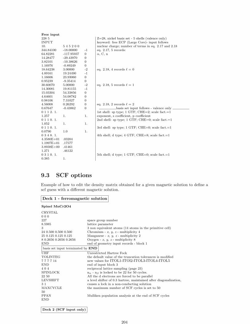
Free input228 5 Z=28, nickel basis set - 5 shells (valence only)INPUT keyword: free ECP (Large Core)- input follows10. 5 4 5 2 0 0 nuclear charge; number of terms in eq. 2.17 and 2.18344.84100 -18.00000 -1 eq. 2.17, 5 records:64.82281 -117.95937 0 α, C, n14.28477 -29.43970 03.82101 -10.38626 01.16976 -0.89249 018.64238 3.00000 -2 eq. 2.18, 4 records ` = 04.89161 19.24490 -11.16606 23.93060 00.95239 -9.35414 030.60070 5.00000 -2 eq. 2.18, 5 records ` = 114.30081 19.81155 -115.03304 54.33856 04.64601 54.08782 00.98106 7.31027 04.56008 0.26292 0 eq. 2.18, 2 records ` = 20.67647 -0.43862 0 basis set input follows - valence only0 1 1 2. 1. 1st shell: sp type; 1 GTF; CHE=2; scale fact.=11.257 1. 1. exponent, s coefficient, p coefficient0 1 1 0. 1. 2nd shell: sp type; 1 GTF; CHE=0; scale fact.=11.052 1. 1.0 1 1 0. 1. 3rd shell: sp type; 1 GTF; CHE=0; scale fact.=10.0790 1.0 1.0 3 4 8. 1. 4th shell; d type; 4 GTF; CHE=8; scale fact.=14.3580E+01 .032041.1997E+01 .175773.8938E+00 .414611.271 .461220 3 1 0. 1. 5th shell; d type; 1 GTF; CHE=0; scale fact.=10.385 1.

9.3 SCF options

Example of how to edit the density matrix obtained for a given magnetic solution to define ascf guess with a different magnetic solution.

Deck 1 - ferromagnetic solution

Spinel MnCr2O4

CRYSTAL0 0 0227 space group number8.5985 lattice parameter3 3 non equivalent atoms (14 atoms in the primitive cell)24 0.500 0.500 0.500 Chromium - x, y, z - multiplicity 425 0.125 0.125 0.125 Manganese - x, y, z - multiplicity 28 0.2656 0.2656 0.2656 Oxygen - x, y, z - multiplicity 8END end of geometry input records - block 1

basis set input terminated by END

UHF Unrestricted Hartree FockTOLINTEG the default value of the truncation tolerances is modified7 7 7 7 14 new values for ITOL1-ITOl2-ITOL3-ITOL4-ITOL5END end of input block 34 0 4 reciprocal lattice sampling (page 23)SPINLOCK nα - nβ is locked to be 22 for 50 cycles.22 50 All the d electrons are forced to be parallelLEVSHIFT a level shifter of 0.3 hartree, maintained after diagonalization,3 1 causes a lock in a non-conducting solutionMAXCYCLE the maximum number of SCF cycles is set to 5050PPAN Mulliken population analysis at the end of SCF cyclesEND

Deck 2 (SCF input only)

204

4 0 4GUESSP initial guess: density matrix from a previous runSPINEDIT elements of the density matrix are modified2 the diagonal elements corresponding to 2 atoms5 6 label of the 2 atoms (6 is equivalent to 5)LEVSHIFT a level shifter of 0.3 hartree, maintained after diagonalization,3 1 causes a lock in a non-conducting solutionPPAN Mulliken population analysis at the end of SCF cyclesEND

=====================================================================First run - geometry output=====================================================================

COORDINATES OF THE EQUIVALENT ATOMS (FRACTIONAL UNITS)

N. ATOM EQUIVALENT AT. NUMBER X Y Z

1 1 1 24 CR -5.000E-01 -5.000E-01 -5.000E-012 1 2 24 CR -5.000E-01 -5.000E-01 0.000E+003 1 3 24 CR 0.000E+00 -5.000E-01 -5.000E-014 1 4 24 CR -5.000E-01 0.000E+00 -5.000E-01

5 2 1 25 MN 1.250E-01 1.250E-01 1.250E-016 2 2 25 MN -1.250E-01 -1.250E-01 -1.250E-01

7 3 1 8 O 2.656E-01 2.656E-01 2.656E-018 3 2 8 O 2.656E-01 2.656E-01 -2.968E-019 3 3 8 O -2.968E-01 2.656E-01 2.656E-01

10 3 4 8 O 2.656E-01 -2.968E-01 2.656E-0111 3 5 8 O -2.656E-01 -2.656E-01 -2.656E-0112 3 6 8 O -2.656E-01 -2.656E-01 2.968E-0113 3 7 8 O -2.656E-01 2.968E-01 -2.656E-0114 3 8 8 O 2.968E-01 -2.656E-01 -2.656E-01

=====================================================================Ferromagnetic solution: all unpaired electrons with the same spin=====================================================================SPIN POLARIZATION - ALPHA-BETA = 22 FOR 50 CYCLES

=====================================================================Convergence on total energy reached in 33 cycles (level shifter active)=====================================================================CYCLE 33 ETOT(AU) -7.072805900367E+03 DETOT -8.168E-07 DE(K) 9.487E+00

=====================================================================Population analysis - ferromagnetic solution=====================================================================MULLIKEN POPULATION ANALYSISALPHA+BETA ELECTRONS - NO. OF ELECTRONS 210.000000

ATOM Z CHARGE SHELL POPULATIONs sp sp sp sp d d

1 CR 24 21.884 2.000 8.047 2.251 4.487 1.331 3.078 .6905 MN 25 23.147 2.000 8.081 2.170 4.299 1.489 4.478 .6297 O 8 9.521 1.996 2.644 2.467 2.414

MULLIKEN POPULATION ANALYSISALPHA-BETA ELECTRONS - NO. OF ELECTRONS 22.000000


1 CR 24 3.057 .000 -.002 .011 .027 -.011 2.790 .2425 MN 25 4.925 .000 -.003 .019 .055 -.052 4.408 .4987 O 8 -.010 .000 .003 -.014 .002

================================================================================================================================================================Second run - Anti ferromagnetic solution:Integrals calculation not affected by the spin state

Cr (atoms 1-2-3-4) unpaired electrons spin alpha;Mn (atoms 5 and 6) unpaired electrons spin beta================================================================================

RESTART FROM A PREVIOUS RUN DENSITY MATRIXSPIN INVERSION IN SPIN DENSITY MATRIX FOR ATOMS: 5 6

=====================================================================Convergence on total energy reached in 15 cycles

205

=====================================================================CYCLE 15 ETOT(AU) -7.072808080821E+03 DETOT -4.930E-07 DE(K) 6.694E-06

======================================uuuu============================Population analysis - anti ferromagnetic solution=====================================================================MULLIKEN POPULATION ANALYSIS

ALPHA+BETA ELECTRONS - NO. OF ELECTRONS 210.000000


1 CR 24 21.884 2.000 8.047 2.251 4.487 1.331 3.078 .6905 MN 25 23.149 2.000 8.081 2.170 4.299 1.489 4.479 .6317 O 8 9.521 1.997 2.644 2.467 2.414

MULLIKEN POPULATION ANALYSISALPHA-BETA ELECTRONS - NO. OF ELECTRONS 2.000000ATOM Z CHARGE SHELL POPULATION

s sp sp sp sp d d1 CR 24 3.049 .000 -.002 .011 .027 -.012 2.785 .2405 MN 25 -4.917 .000 .003 -.018 -.055 .054 -4.406 -.4957 O 8 -.045 .000 -.024 -.013 -.008

================================================================================

9.4 Geometry optimization

Crystal geometry input section (block1) for the geometry optimization of the urea molecule:

. Example

Urea Molecule TitleMOLECULE Dimension of the system15 Point group (C2v)5 Number of non equivalent atoms6 0. 0. 0. Atomic number and cartesian coordinates8 0. 0. 1.2614017 0. 1.148247 -0.6997901 0. 2.026550 -0.2028171 0. 1.134080 -1.704975OPTGEOM Keyword to perform a geometry optimizationENDOPT End of geometry optimization input blockEND end og geometry inputBasis set input As in test 12END End of basis set input sectionEND block3 input - Molecule - no information on sampling in K space

Crystal output contains additional information on the optimization run after the initial partof the geometry output:

. . . . . . . . .. . . . . . . . . . . . . . . . . .

BERNY OPTIMIZATION CONTROL

MAXIMUM GRADIENT COMPONENT 0.00045 MAXIMUM DISPLACEMENT COMPONENT 0.00030R.M.S. OF GRADIENT COMPONENT 0.00180 R.M.S. OF DISPLACEMENT COMPONENTS 0.00120THRESHOLD ON ENERGY CHANGE 0.100E-06 EXTRAPOLATING POLYNOMIAL ORDER 2MAXIMUM ALLOWED NUMBER OF STEPS 100 SORTING OF ENERGY POINTS: NOANALYTICAL GRADIENTS. . . . . . . . .. . . . . . . . . . . . . . . . . .

SYMMETRY ALLOWED INTERNAL DEGREE(S) OF FREEDOM: 7

. . . . . . . . .. . . . . . . . . . . . . . . . . .

206

At the first step of the optimization, the Crystal standard output contains both energy(complete SCF cycle) and gradient parts. At the end of the first step, a convergence check isperformed on the initial forces and the optimization stops if the criteria are already satisfied.For the subsequent steps, only few lines on the optimization process are reported in standardoutput, namely: current geometry, total energy and gradients, and convergence tests (SCFoutput is routed to file SCFOUT.LOG).At each optimization step, xxx, the geometry is written in file optcxxx (in a format suitableto be read with EXTERNAL keyword). Optimization step can be restarted from any stepgeometry, by renaming optcxxx as fort.34.The standard output for the urea molecule geometry optimization looks as follows:

OPTOPTOPTOPTOPTOPTOPTOPTOPTOPTOPTOPTOPTOPTOPTOPTOPTOPTOPTOPTOPTOPTOPTOPTOPTOPT*******************************************************************************GEOMETRY OPTIMIZATION - POINT 2*******************************************************************************ATOMS IN THE ASYMMETRIC UNIT 5 - ATOMS IN THE UNIT CELL: 8

ATOM X(ANGSTROM) Y(ANGSTROM) Z(ANGSTROM)*******************************************************************************

1 T 6 C 0.000000000000E+00 0.000000000000E+00 2.645266012706E-022 T 8 O 0.000000000000E+00 0.000000000000E+00 1.241474126876E+003 T 7 N 0.000000000000E+00 1.150483100972E+00 -7.044307566681E-014 F 7 N 0.000000000000E+00 -1.150483100972E+00 -7.044307566681E-015 T 1 H 0.000000000000E+00 2.022583078191E+00 -2.043778206895E-016 F 1 H 0.000000000000E+00 -2.022583078191E+00 -2.043778206895E-017 T 1 H 0.000000000000E+00 1.135517317174E+00 -1.702036316144E+008 F 1 H 0.000000000000E+00 -1.135517317174E+00 -1.702036316144E+00

T = ATOM BELONGING TO THE ASYMMETRIC UNIT

INTRACELL NUCLEAR REPULSION (A.U.) 1.2463005288098E+02

TOTAL ENERGY(HF)(AU)( 11) -2.2379435865343E+02 DE-4.8E-08 DP 7.2E-06

SYMMETRY ALLOWED FORCES (ANALYTICAL) (DIRECTION, FORCE)

1 4.0854048E-02 2 -2.8460660E-02 3 1.4184257E-03 4 -3.0361419E-035 -1.7599295E-02 6 -1.3809310E-02 7 6.7962224E-03

GRADIENT NORM 0.055108 GRADIENT THRESHOLD 0.500000

MAX GRADIENT 0.040854 THRESHOLD 0.000450 CONVERGED NORMS GRADIENT 0.020829 THRESHOLD 0.000300 CONVERGED NOMAX DISPLAC. 0.024990 THRESHOLD 0.001800 CONVERGED NORMS DISPLAC. 0.015649 THRESHOLD 0.001200 CONVERGED NO

When all four convergence tests are satisfied, optimization is completed. The final energy andthe optimized structure are printed after the final convergence tests.

******************************************************************* OPT END - CONVERGED * E(AU): -2.237958289701E+02 POINTS 14 *******************************************************************

. . . . . . . . . . . . . . . . . . . . . . . . . . . . . . .. . .

FINAL OPTIMIZED GEOMETRY - DIMENSIONALITY OF THE SYSTEM 0(NON PERIODIC DIRECTION: LATTICE PARAMETER FORMALLY SET TO 500)*******************************************************************************ATOMS IN THE ASYMMETRIC UNIT 5 - ATOMS IN THE UNIT CELL: 8

ATOM X(ANGSTROM) Y(ANGSTROM) Z(ANGSTROM)*******************************************************************************

1 T 6 C 0.000000000000E+00 0.000000000000E+00 3.468988750953E-022 T 8 O 0.000000000000E+00 0.000000000000E+00 1.230143233209E+003 T 7 N 0.000000000000E+00 1.143750090534E+00 -7.056136525307E-014 F 7 N 0.000000000000E+00 -1.143750090534E+00 -7.056136525307E-015 T 1 H 0.000000000000E+00 2.001317638364E+00 -2.076003454226E-016 F 1 H 0.000000000000E+00 -2.001317638364E+00 -2.076003454226E-017 T 1 H 0.000000000000E+00 1.157946292824E+00 -1.696084062406E+00

207

8 F 1 H 0.000000000000E+00 -1.157946292824E+00 -1.696084062406E+00

T = ATOM BELONGING TO THE ASYMMETRIC UNIT

INTRACELL NUCLEAR REPULSION (A.U.) 1.2541002823701E+02

**** 4 SYMMOPS - TRANSLATORS IN FRACTIONA LUNITSV INV ROTATION MATRICES TRANSLATOR1 1 1.00 0.00 0.00 0.00 1.00 0.00 0.00 0.00 1.00 0.00 0.00 0.002 2 -1.00 0.00 0.00 0.00 -1.00 0.00 0.00 0.00 1.00 0.00 0.00 0.003 3 -1.00 0.00 0.00 0.00 1.00 0.00 0.00 0.00 1.00 0.00 0.00 0.004 4 1.00 0.00 0.00 0.00 -1.00 0.00 0.00 0.00 1.00 0.00 0.00 0.00

The final geometry is both printed in the Crystal output and writ-ten in file fort.34. The following input defines the geometry, read-ing data from file fort.34 (keyword EXTERNAL, input block1, page 15).

. Example

Urea Molecule TitleEXTERNAL Geometry read from file fort.34optional keywordsEND End of the geometry input section

Optimization can restart, by adding the keyword RESTART in the sameinput deck used for the first optimization run. Information to restartare read from file OPTINFO.DAT, updated after each optimization cycle.

. Example

Initial input Restart input

Urea Molecule Urea MoleculeMOLECULE MOLECULE15 155 56 0. 0. 0. 6 0. 0. 0.8 0. 0. 1.261401 8 0. 0. 1.2614017 0. 1.148247 -0.699790 7 0. 1.148247 -0.6997901 0. 2.026550 -0.202817 1 0. 2.026550 -0.2028171 0. 1.134080 -1.704975 1 0. 1.134080 -1.704975OPTGEOM OPTGEOMENDOPT RESTARTEND ENDOPT

END

Partial optimization

In order to optimize the coordinates of the hydrogens in urea molecule, the following inputmust be entered:

208

. Example

Urea Molecule TitleMOLECULE Dimension of the system15 Point group (C2v)5 Number of non equivalent atoms6 0. 0. 0. Atomic number and cartesian coordinates8 0. 0. 1.2614017 0. 1.148247 -0.6997901 0. 2.026550 -0.2028171 0. 1.134080 -1.704975KEEPSYMM maintain symmetry in subsequent operationsOPTGEOM Keyword to perform a geometry optimizationFRAGMENT Keyword for a partial optimization2 Number of atoms to be optimized5 7 Label of the atoms to be optimizedENDOPT End of the geometry optimization input blockEND End of the geometry input section

The atoms allowed to move are the two hydrogens irreducible, 5 and 7. The symmetry ismaintained, atoms 6 and 7 are allowed to move.

******************************************************************************** PARTIAL OPTIMIZATION - ATOMS FREE TO MOVE 2 INPUT LIST :

5( 1) 7( 1)

SYMMETRY IS KEPT

ATOM 5 AND 6 ARE LINKED BY SYMMOP 2ATOM 7 AND 8 ARE LINKED BY SYMMOP 2*******************************************************************************

If the symmetry is not maintained (default, no KEEPSYMM before OPTGEOM) the symmetryoperators linking atoms 5 and 6, and atoms 7 and 8, are removed.

******************************************************************************** PARTIAL OPTIMIZATION - ATOMS FREE TO MOVE 2 INPUT LIST :

5( 1) 7( 1)

SYMMETRY MAY BE BROKEN

THE NUMBER OF SYMMETRY OPERATORS HAS BEEN REDUCED FROM 4 TO 2******************************************************************************

. . . . . . . . . . . . . . . . . . . . . . . . . . . . . . .. . .SYMMETRY ALLOWED INTERNAL DEGREE(S) OF FREEDOM: 4. . . . . . . . . . . . . . . . . . . . . . . . . . . . . . .. . .

Final run

During optimization process, the classification of the integrals is done with reference to theinput geometry, and used for all subsequent wave function calculations.In some cases, when the optimized geometry is far from the original one, the series truncationdefined with reference to the starting geometry may be inhomogeneous if applied to the finalgeometry (see keyword FIXINDEX for explanation). In those cases, the total energy com-puted for one geometry, with integrals selected according to a different geometry, may be notcorrect.A single point calculation, with the final optimized geometry, allows to check if that is thecase.

209

A safe procedure to check if that geometry corresponds to a real energy minimum, is to per-form a second optimization process, with same truncation criteria, starting from the geometryobtained in the first optimization (read from file fort.34, keyword EXTERNAL, page 15).The keyword FINALRUN starts the process automatically. (it does not work with Pcrystal)

A typical example is the geometry optimization of a surface, described with a slabmodel. The optimization process may lead to a structure significantly differentfrom the one cut from the bulk, when there is surface relaxation. As an exam-ple, the geometry optimization of the surface (001) of the α -Al2O3 is reported.

. Example - Optimization of surface

α -Al2O3 - (001) surface titleCRYSTAL dimension of the system0 0 0167 space group4.7602 12.9933 lattice parameters2 number of irreducible atoms13 0. 0. 0.35216 fractional coordinates of first atom8 0.30624 0. 0.25 fractional coordinates of second atomSLABCUT 3D→ 2D0 0 1 (h, k, l) Miller indices of the surface1 6 number of layers, starting from the first classifiedOPTGEOM Keyword to perform a geometry optimizationFINALRUN keyword to check gradients vs true series truncation3 new optimization if convergence criteria are not satisfiedENDOPT end of the geometry optimization input blockEND end of the geometry input section

Neighbors analysis on the initial geometry obtained with SLABCUT

N = NUMBER OF NEIGHBORS AT DISTANCE R 11 cycles

ATOM N R/ANG R/AU NEIGHBORS (ATOM LABELS AND CELL INDICES)

1 AL 3 1.8551 3.5057 2 O 0 0 0 3 O 0 0 0 4 O 0 1 0

1 AL 3 3.2192 6.0834 5 AL 0 0 0 5 AL 1 1 0 5 AL 0 1 0

1 AL 3 3.2219 6.0885 2 O -1 0 0 3 O 1 1 0 4 O 0 0 0

1 AL 3 3.4295 6.4808 7 O 0 1 0 8 O 0 1 0 9 O 0 0 0

1 AL 3 3.4990 6.6121 6 AL 0 0 0 6 AL -1 0 0 6 AL 0 1 0

1 AL 1 3.8419 7.2601 10 AL 0 0 0

Total energy E = -1399.7999027 hartree

Series truncation is defined with reference to that geometry. Optimization begins. After 11cycles convergence on gradients and displacements is satisfied.Neighbors analysis on the optimized geometry:

N = NUMBER OF NEIGHBORS AT DISTANCE Ra 6 cycles


1 AL 3 1.6886 3.1911 2 O 0 0 0 3 O 0 0 0 4 O 0 1 0

1 AL 1 2.6116 4.9351 10 AL 0 0 0

1 AL 3 2.8198 5.3286 7 O 0 1 0 8 O 0 1 0 9 O 0 0 0

1 AL 3 3.0425 5.7494 5 AL 0 0 0 5 AL 1 1 0 5 AL 0 1 0

210

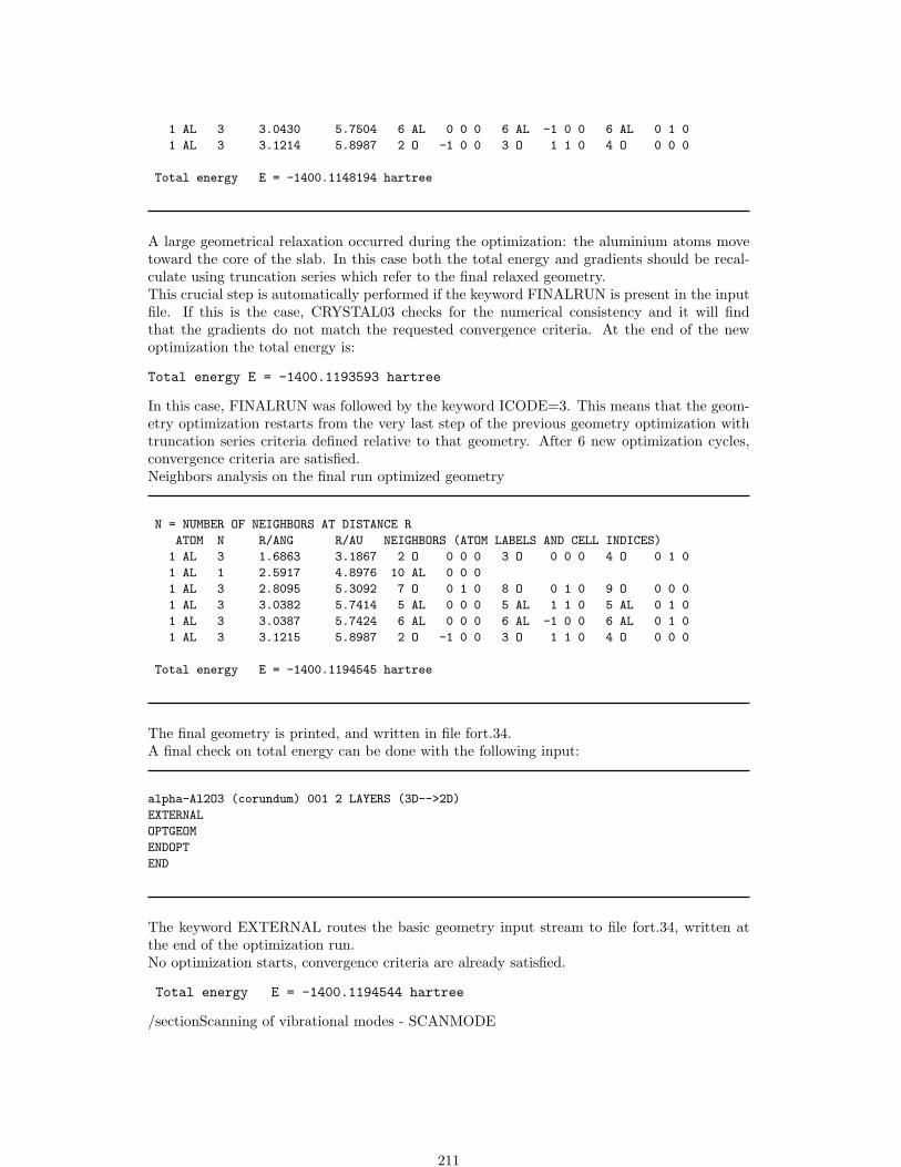
1 AL 3 3.0430 5.7504 6 AL 0 0 0 6 AL -1 0 0 6 AL 0 1 0

1 AL 3 3.1214 5.8987 2 O -1 0 0 3 O 1 1 0 4 O 0 0 0


A large geometrical relaxation occurred during the optimization: the aluminium atoms movetoward the core of the slab. In this case both the total energy and gradients should be recal-culate using truncation series which refer to the final relaxed geometry.This crucial step is automatically performed if the keyword FINALRUN is present in the inputfile. If this is the case, CRYSTAL03 checks for the numerical consistency and it will findthat the gradients do not match the requested convergence criteria. At the end of the newoptimization the total energy is:


In this case, FINALRUN was followed by the keyword ICODE=3. This means that the geom-etry optimization restarts from the very last step of the previous geometry optimization withtruncation series criteria defined relative to that geometry. After 6 new optimization cycles,convergence criteria are satisfied.Neighbors analysis on the final run optimized geometry

N = NUMBER OF NEIGHBORS AT DISTANCE R


1 AL 3 1.6863 3.1867 2 O 0 0 0 3 O 0 0 0 4 O 0 1 0

1 AL 1 2.5917 4.8976 10 AL 0 0 0

1 AL 3 2.8095 5.3092 7 O 0 1 0 8 O 0 1 0 9 O 0 0 0

1 AL 3 3.0382 5.7414 5 AL 0 0 0 5 AL 1 1 0 5 AL 0 1 0

1 AL 3 3.0387 5.7424 6 AL 0 0 0 6 AL -1 0 0 6 AL 0 1 0

1 AL 3 3.1215 5.8987 2 O -1 0 0 3 O 1 1 0 4 O 0 0 0


The final geometry is printed, and written in file fort.34.A final check on total energy can be done with the following input:

alpha-Al2O3 (corundum) 001 2 LAYERS (3D-->2D)

EXTERNAL

OPTGEOM

ENDOPT

END

The keyword EXTERNAL routes the basic geometry input stream to file fort.34, written atthe end of the optimization run.No optimization starts, convergence criteria are already satisfied.


/sectionScanning of vibrational modes - SCANMODE

211

Methane molecule

MOLECULE4426 0.000000000000E+00 0.000000000000E+00 0.000000000000E+001 6.252140000000E-01 6.252140000000E-01 6.252140000000E-01FREQCALCSCANMODE-1 -1 0 0.112ENDfreqEND6 30 0 3 2. 1.172.256000 0.617669000E-0125.9109000 0.3587940005.53335000 0.7007130000 1 2 4. 1.3.66498000 -0.395897000 0.2364600000.770545000 1.21584000 0.8606190000 1 1 0. 1.0.195857000 1.00000000 1.000000001 20 0 2 1. 1.5.44717800 0.1562850000.824547000 0.9046910000 0 1 0. 1.0.183192000 1.0000000099 0ENDTOLINTEG20 20 20 20 20ENDTOLDEE11END

PbCO3

PBCO3 - frequency calculationCRYSTAL1 0 0P m c n5.20471446 8.45344758 6.160741454282 2.500000000000E-01 4.175726169487E-01 -2.463557995068E-016 2.500000000000E-01 -2.363341497085E-01 -8.558132726424E-028 2.500000000000E-01 -8.360585350428E-02 -9.431628799197E-028 4.648370653436E-01 -3.129222129903E-01 -8.842925698155E-02FREQCALCRESTARTSCANMODE1 -40 40 0.11END

212

END282 4HAYWLC0 1 2 4. 1.1.335104 -0.1448789 -0.10706120.7516086 1.0 1.0

0 1 1 0. 1.0.5536686 1.0 1.0

0 1 1 0. 1.0.1420315 1.0 1.0

0 3 1 0. 1.0.1933887 1.0

6 40 0 6 2.0 1.03048.0 0.001826456.4 0.01406103.7 0.0687629.23 0.23049.349 0.46853.189 0.3628

0 1 2 4.0 1.03.665 -0.3959 0.23650.7705 1.216 0.8606

0 1 1 0.0 1.00.26 1.0 1.0

0 3 1 0.0 1.00.8 1.0

8 40 0 6 2.0 1.0

.5484671660D+04 .1831074430D-02

.8252349460D+03 .1395017220D-01

.1880469580D+03 .6844507810D-01

.5296450000D+02 .2327143360D+00

.1689757040D+02 .4701928980D+00

.5799635340D+01 .3585208530D+000 1 3 6.0 1.0

.1553961625D+02 -.1107775490D+00 .7087426820D-01

.3599933586D+01 -.1480262620D+00 .3397528390D+00

.1013761750D+01 .1130767010D+01 .7271585770D+000 1 1 0.0 1.0

.2700058226D+00 .1000000000D+01 .1000000000D+010 3 1 0.0 1.0

.8000000000D+00 .1000000000D+0199 0ENDBSSCFDIRDFTB3LYPRADIAL14.099ANGULAR50.1667 0.5 0.9 3.5 9999.06 10 14 18 14END

213

SHRINK6 6LEVSHIFT5 0TOLDEE10MAXCYCLE200ENDSCF

214

Chapter 10

Basis set

The most common source of problems with CRYSTAL is probably connected with the basis set.It should never be forgotten that ultimately the basis functions are Bloch functions, modulatedover the infinite lattice: any attempt to use large uncontracted molecular or atomic basis sets,with very diffuse functions can result in the wasting of computational resources. The denselypacked nature of many crystalline structures gives rise to a large overlap between the basisfunctions, and a quasi-linear dependence can occur, due to numerical limitations.The choice of the basis set (BS) is one of the critical points, due to the large variety ofchemical bonding that can be found in a periodic system. For example, carbon can be involvedin covalent bonds (polyacetylene, diamond) as well as in strongly ionic situations (Be2C, wherethe Mulliken charge of carbon is close to -4).Many basis sets for lighter elements and the first row transition metal ions have been developedfor use in periodic systems. A selection of these which have been used in published work areavailable on WWW:


We summarize here some general considerations which can be useful in the construction of aBS for periodic systems.It is always useful to refer to some standard basis set; Pople’s STO-nG, 3-21G and 6-21G haveproved to be good starting points. A molecular minimal basis set can in some cases be usedas it is; larger basis sets must be re-optimized specifically for the chemical periodic structureunder study.Let us explore the adequacy of the molecular BS for crystalline compounds and add someconsiderations which can be useful when a molecular BS must be modified or when an ex novocrystalline BS is defined.

10.1 Molecular BSs performance in periodic systems

Two sets of all electron basis sets are included in CRYSTAL (see Chapter 1.2):

1. Minimal STO-nG basis set of Pople and co-workersobtained by fitting Slater type orbitals with n contracted GTFs (n from 2 to 6, atomicnumber from 1 to 54) [73, 72, 98, 97].The above BSs are still widely used in spite of the poor quality of the resulting wave func-tion, because they are well documented and as a rule provide quite reasonable optimizedgeometries (due to fortuitous cancellation of errors) at low cost.

2. ”Split valence” 3-21 and 6-21 BSs.The core shells are described as a linear combination of 3 (up to atomic number 54)or 6 (up to atomic number 18) gaussians; the two valence shells contain two and onegaussians, respectively [15, 60]. Exponents (s and p functions of the same shell share thesame exponent) and contraction coefficients have been optimized variationally for theisolated atoms.

215

A single set of polarization functions (p,d) can be added without causing numerical problems.Standard molecular polarization functions are usually also adequate for periodic compounds.

When free basis sets are chosen, two points should be taken into account:

1. From the point of view of CPU time, basis sets with sp shells (s and p functions sharingthe same set of exponents) can give a saving factor as large as 4, in comparison withbasis sets where s and p have different exponents.

2. As a rule, extended atomic BSs, or ’triple zeta’ type BSs should be avoided. Many ofthe high quality molecular BSs (Roos, Dunning, Huzinaga) cannot be used in CRYSTALwithout modification, because the outer functions are too diffuse. One should not forgetthat the real basis functions are Bloch functions.

Let us consider in more detail the possibility of using molecular BS for periodic systems. Wecan refer to five different situations:

Core functionsValence functions: molecular crystals

covalent crystalsionic crystalsmetals.

10.2 Core functions

In this case standard (contracted) molecular BSs can be adopted without modification, be-cause even when very strong crystal field effects are present, the deformation of inner statesis small, and can be correctly described through the linear variational parameters in SCF cal-culation. An adequate description of the core states is important in order to avoid large basisset superposition errors.

10.3 Valence functions

Molecular crystals

Molecular BSs, minimal and split-valence, are perfectly adequate. Tests have been performedon bulk urea [36] and oxalic acid, where the molecules are at relatively small distances, withSTO-3G, 6-21, 6-21* and 6-21** BSs presenting no problem.

Covalent crystals.

Standard minimal and split valence BSs are usually adequate. In the split valence case thebest exponent of the most diffuse shell is always slightly higher than the one proposed formolecules; in general it is advisable to re-optimize the exponent of this shell. This produces aslightly improved basis, while reducing the cost of the calculation. Let us consider for examplethe 6-21 basis set for carbon (in diamond) and silicon (bulk).At an atomic level, the best exponent of the outer shell is 0.196 and 0.093 for C and Si, respec-tively. Optimization of the valence shell has been repeated in the two crystalline compounds.The innermost valence shell is essentially unaltered with respect to the atomic solution; for theouter single-gaussian shell the best exponent is around 0.22 and 0.11 bohr−2 for carbon andsilicon, as shown in Table 10.1. The last entry of Table 10.1 refers to ”catastrophic” behaviour:the low value of the exponent generates unphysical states.A set of 5 polarization single-gaussian d functions can be added to the 6-21G basis (6-21G*BS); the best exponents for the solid are very close to those resulting from the optimization inmolecular contexts: 0.8 for diamond [66] and 0.45 for silicon.

Basis sets for III-V and IV-IV semiconductors (all electron and valence electron (to be associ-ated with effective core pseudopotentials) are given in references [86, 26].

216

Table 10.1: Total energy per cell and number of computed bielectronic integrals in 106 units(N), as a function of the exponent α (bohr−2) of the most diffuse shell for carbon and silicon.____________________________________________________________________

Diamond Silicon------------------------ --------------------------a N Et a N Et___________________________________________________________0.296 58 -75.6633 0.168 46 -577.80990.276 74 -75.6728 0.153 53 -577.81810.256 83 -75.6779 0.138 72 -577.82310.236 109 -75.6800 0.123 104 -577.82680.216 148 -75.6802 0.108 151 -577.82760.196 241 -75.6783 0.093 250 -577.82660.176 349 catastrophe 0.078 462 catastrophe

____________________________________________________________________

Ionic crystals.

Cations

The classification of covalent or ionic crystals is highly conventional, many systems beingmidway. Let us first consider totally ionic compounds, such as LiH, MgO, or similar. For thesesystems the cation valence shell is completely empty. Therefore, for cations it is convenientto use a basis set containing the core functions plus an additional sp shell with a relativelyhigh exponent. For example, we used for Mg in MgO and for Li in LiH ( Li2 O and Li3 N) a’valence’ sp shell with exponent 0.4-0.3 and 0.5-0.6, respectively [41, 25].The crystalline total energies obtained by using only core functions for Li or Mg and by addinga valence shell to the cation differ by 0.1 eV/atom, or less. This figure is essentially the samefor a relatively large range of exponents of the valence shell (say 0.5-0.2 for Mg) [25].It can be difficult (or impossible) to optimize the exponents of nearly empty shells: the en-ergy decreases almost linearly with the exponent. Very low exponent values can give rise tonumerical instabilities, or require the calculation of an enormous number of integrals (selectedon the basis of overlap criteria). In the latter cases, when the energy gain is small (∆E ≤ 1 mhartree for ∆α = 0.2 bohr−2), it is convenient to use a relatively large exponent.

Anions

Reference to isolated ion solutions is only possible for halides, because in such cases the ionsare stable even at the HF level. For other anions, which are stabilized by the crystallinefield (H−, O2−, N3− and also C4−), the basis set must be re-designed with reference to thecrystalline environment. For example, let us consider the optimization of the O2− BS in Li2O[41]. Preliminary tests indicated the fully ionic nature of the compound; the point was then toallow the valence distribution to relax in the presence of the two extra electrons. We startedfrom a standard STO-6G BS. Two more gaussians were introduced in the 1s contraction, inorder to improve the virial coefficient and total energy, as a check of wave function quality. The6 valence gaussians were contracted according to a 411 scheme; the exponents of the two outerindependent gaussians and the coefficients of the four contracted ones were optimized. Whereasthe two most diffuse gaussians are more diffuse than in the neutral isolated atom (α=0.45 and0.15 to be compared with α=0.54 and 0.24 respectively), the rest of the O2− valence shell isunchanged with respect to the atomic situation. The introduction of d functions in the oxygenbasis-set causes only a minor improvement in energy (1 10−4 hartree/cell, with a populationof 0.02 electrons/atom in the cell). Ionic BSs for H and N can be found in reference 1.For anions, re-optimization of the most diffuse valence shell is mandatory; when starting froma standard basis set, the most diffuse (or the two most diffuse) gaussians must be allowed torelax.

217

From covalent to ionics

Intermediate situations must be considered individually, and a certain number of tests mustbe performed in order to verify the adequacy of the selected BSs.Let us consider for example α-quartz (SiO2) and corundum (Al2O3). The exponent of theouter shell for the 2 cations in the 6-21G BS is 0.093 (Si) and 0.064 (Al), respectively; in bothcases this function is too diffuse (in particular in the Al case it causes numerical catastrophes).For quartz, re-optimization in the bulk gives α=0.15 bohr−2 for Si (the dependence of totalenergy per Si atom on α is much smaller than the one resulting from Table 10.1; note too thatthe cost at α=0.15 is only 50% of the one at α=0.09). On the contrary, the best molecularand crystalline exponent (α=0.37) for oxygen coincide. Corundum is more ionic than quartz,and about 2 valence electrons are transferred to oxygen. In this case it is better to eliminatethe most diffuse valence shell of Al, and to use as independent functions the two gaussians ofthe inner valence shells (α=0.94 and 0.20 bohr−2, respectively [109]).

Metals

Very diffuse gaussians are required to reproduce the nearly uniform density characterizingsimple metallic systems, such as lithium and beryllium. This is the worse situation, where afull optimization of the atomic basis set is probably impossible. Functions which are too diffusecan create numerical problems, as will be discussed below.The optimization procedure can start from 6-21 BS; the most diffuse valence shell (exponent0.028 for Li and 0.077 for Be) can be dropped and the innermost valence shell (exponents 0.54and 0.10 for Li, and 1.29 and 0.268 for Be) can be split.

Table 10.2: Example of BS for metallic lithium and beryllium derived from the standard 6-21GBS

.

_______________________________________________________________Lithium Beryllium

shell Exp. Coeff. shell Exp. Coeff._______________________________________________________________s 642.418 0.00215096 s 1264.50 0.00194336

96.5164 0.0162677 189.930 0.014825122.0174 0.0776383 43.1275 0.07206626.1764 0.246495 12.0889 0.2370221.93511 0.467506 3.80790 0.468789

sp 0.640 1. 1. 1.282 1. 1.sp 0.10 1. 1. 0.27 1. 1.

_______________________________________________________________

At this point the outer gaussian of the 6G core contraction, with very similar exponents (0.64and 1.28) to those of the innermost valence shell (0.54 and 1.29), can be used as an independent(sp) function, and the innermost valence shell can be eliminated.The resulting (reasonable) BS, derived from the split valence standard one, is reported in Table10.2. Finally, the most diffuse gaussian can be optimized; in the two cases the minimum hasnot been found owing to numerical instabilities.See [37] for a more extensive discussion of the metallic lithium case.

10.4 Hints on crystalline basis set optimization

In the definition of a valence shell BS, each exponent can be varied in a relatively narrow range:in the direction of higher exponents, large overlaps with the innermost functions may occur(the rule of thumb is: exponents must be in a ratio not too far from 3; ratios smaller than

218

2 can give linear dependence problems); proceeding towards lower exponents, one must avoidlarge overlaps with a high number of neighbours (remember: the basis functions are Blochfunctions).Diffuse gaussian orbitals play a critical role in HF-LCAO calculations of crystals, especiallythe three-dimensional ones; they are expensive, not always useful, in some cases dangerous.

• Cost.

The number of integrals to be calculated increases dramatically with decreasing exponents;this effect is almost absent in molecular calculations. Table 10.1 shows that the cost of thecalculation (number of bielectronic integrals) for silicon (diamond) can increase by a factor10 (6) simply by changing the exponent of the most diffuse single-gaussian from 0.168 to0.078 (0.296 to 0.176). The cost is largely dominated by this shell, despite the fact that largecontractions are used for the 1s, 2sp and the innermost valence shell.A high number of contracted primitives tremendously increases the integrals computation time.

• Usefulness.

In atoms and molecules a large part of the additional variational freedom provided by diffusefunctions is used to describe the tails of the wave function, which are poorly represented by thee−αr2

decay of the gaussian function. On the contrary, in crystalline compounds (in particular3D non-metallic systems), low exponent functions do not contribute appreciably to the wavefunction, due to the large overlap between neighbours in all directions. A small split valenceBS such as the 6-21G one, is nearer to the variational limit in crystals than in molecules.

• Numerical accuracy and catastrophic behaviour.

In some conditions, during the SCF (periodic) calculation, the system ’falls’ into non-physicalstates, characterized by very low single particle and total energies (see for example the lastentry in Table 10.1 and the above discussion on metals).This behaviour, generically interpreted in our early papers as due to ’linear dependence’, isactually due to poor accuracy in the treatment of the Coulomb and exchange series. Theexchange series is much more delicate, for two reasons: first, long range contributions are nottaken into account (whereas the long range Coulomb contributions are included, although in anapproximate way); second, the ”pseudoverlap” criteria associated with the two computationalparameters ITOL4 and ITOL5 mimic only in an approximate way the real behaviour of thedensity matrix.The risks of ”numerical catastrophes” increase rapidly with a decreasing exponent; higherprecision is required in order to obtain physical solutions.For non-metallic systems, and split-valence type BSs, the default computational conditionsgiven in section 1.3 are adequate for the optimization of the exponents of the valence shell andfor systematic studies of the energy versus volume curves.For metallic systems, the optimization of the energy versus exponent curve could require ex-tremely severe conditions for the exchange series and, as a consequence, for the reciprocalspace net. Reasonable values of the valence shell exponent (say 0.23 for beryllium and 0.10for lithium, see Table 10.2), though not corresponding to a variational minimum, are reason-ably adequate for the study of the structural and electronic properties of metallic systems (seereference 1).

10.5 Check on basis-set quasi-linear-dependence

In order to check the risk of linear dependence of Bloch functions, it is possible to calculatethe eigenvalues of the overlap matrix in reciprocal space by running integrals and enteringthe keyword EIGS (input block 3, page 81). Full input (general information, geometry, basisset, SCF) is to be entered.

219

The overlap matrix in direct space is Fourier transformed at all the k points generated in theirreducible part of the Brillouin zone, and diagonalized. The eigenvalues are printed.The higher the numerical accuracy obtained by severe computational conditions, the closerto 0 can be the eigenvalues without risk of numerical instabilities. Negative values indicatenumerical linear dependence. The program stops after the check (even if negative eigenvaluesare not detected).The Cholesky reduction scheme [77] requires basis functions linearly independent. A symptomof numerical dependence may produce an error message in RHOLSK or CHOLSK while runningscf.

220

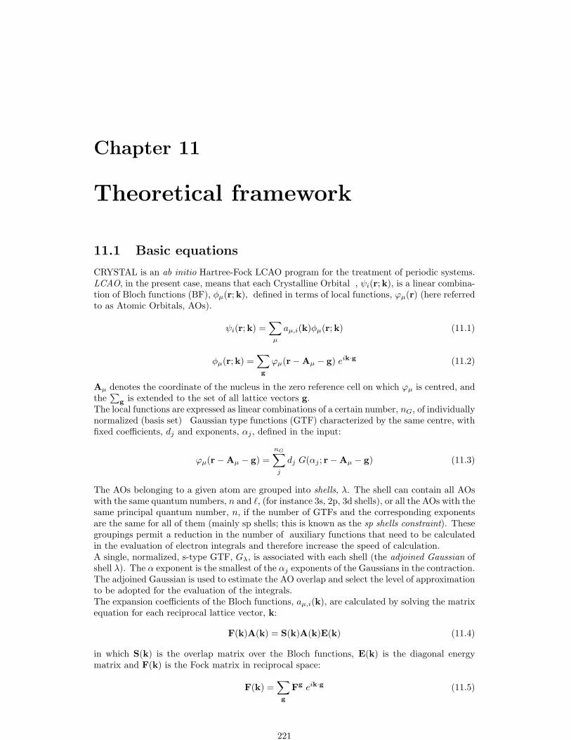
Chapter 11

Theoretical framework

11.1 Basic equations

CRYSTAL is an ab initio Hartree-Fock LCAO program for the treatment of periodic systems.LCAO, in the present case, means that each Crystalline Orbital , ψi(r;k), is a linear combina-tion of Bloch functions (BF), φµ(r;k), defined in terms of local functions, ϕµ(r) (here referredto as Atomic Orbitals, AOs).

ψi(r;k) =∑

µ

aµ,i(k)φµ(r;k) (11.1)

φµ(r;k) =∑g

ϕµ(r−Aµ − g) eik·g (11.2)

Aµ denotes the coordinate of the nucleus in the zero reference cell on which ϕµ is centred, andthe

∑g is extended to the set of all lattice vectors g.

The local functions are expressed as linear combinations of a certain number, nG, of individuallynormalized (basis set) Gaussian type functions (GTF) characterized by the same centre, withfixed coefficients, dj and exponents, αj , defined in the input:

ϕµ(r−Aµ − g) =nG∑j

dj G(αj ; r−Aµ − g) (11.3)

The AOs belonging to a given atom are grouped into shells, λ. The shell can contain all AOswith the same quantum numbers, n and `, (for instance 3s, 2p, 3d shells), or all the AOs with thesame principal quantum number, n, if the number of GTFs and the corresponding exponentsare the same for all of them (mainly sp shells; this is known as the sp shells constraint). Thesegroupings permit a reduction in the number of auxiliary functions that need to be calculatedin the evaluation of electron integrals and therefore increase the speed of calculation.A single, normalized, s-type GTF, Gλ, is associated with each shell (the adjoined Gaussian ofshell λ). The α exponent is the smallest of the αj exponents of the Gaussians in the contraction.The adjoined Gaussian is used to estimate the AO overlap and select the level of approximationto be adopted for the evaluation of the integrals.The expansion coefficients of the Bloch functions, aµ,i(k), are calculated by solving the matrixequation for each reciprocal lattice vector, k:

F(k)A(k) = S(k)A(k)E(k) (11.4)

in which S(k) is the overlap matrix over the Bloch functions, E(k) is the diagonal energymatrix and F(k) is the Fock matrix in reciprocal space:

F(k) =∑g

Fg eik·g (11.5)

221

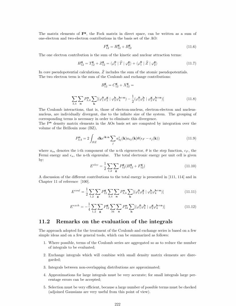
The matrix elements of Fg, the Fock matrix in direct space, can be written as a sum ofone-electron and two-electron contributions in the basis set of the AO:

F g12 = Hg

12 +Bg12 (11.6)

The one electron contribution is the sum of the kinetic and nuclear attraction terms:

Hg12 = T g

12 + Zg12 = 〈ϕ0

1 | T | ϕg2 〉+ 〈ϕ0

1 | Z | ϕg2 〉 (11.7)

In core pseudopotential calculations, Z includes the sum of the atomic pseudopotentials.The two electron term is the sum of the Coulomb and exchange contributions:

Bg12 = Cg

12 +Xg12 =

∑3,4

∑n

Pn3,4

∑h

[(ϕ01ϕ

g2 | ϕh

3ϕh+n4 )− 1

2(ϕ0

1ϕh3 | ϕ

g2ϕ

h+n4 )] (11.8)

The Coulomb interactions, that is, those of electron-nucleus, electron-electron and nucleus-nucleus, are individually divergent, due to the infinite size of the system. The grouping ofcorresponding terms is necessary in order to eliminate this divergence.The Pn density matrix elements in the AOs basis set are computed by integration over thevolume of the Brillouin zone (BZ),

Pn3,4 = 2

∫BZ

dkeik·n∑

j

a∗3j(k)a4j(k)θ(εF − εj(k)) (11.9)

where ain denotes the i-th component of the n-th eigenvector, θ is the step function, εF , theFermi energy and εn, the n-th eigenvalue. The total electronic energy per unit cell is givenby:

Eelec =12

∑1,2

∑g

P g12(H

g12 + F g

12) (11.10)

A discussion of the different contributions to the total energy is presented in [111, 114] and inChapter 11 of reference [100].

Ecoul =12

∑1,2

∑g

P g12

∑3,4

∑n

Pn3,4

∑h

[(ϕ01ϕ

g2 | ϕh

3ϕh+n4 )] (11.11)

Eexch = −14

∑1,2

∑g

P g12

∑34

∑n

Pn34

∑h

[(ϕ01ϕ

h3 | ϕ

g2ϕ

h+n4 )] (11.12)

11.2 Remarks on the evaluation of the integrals

The approach adopted for the treatment of the Coulomb and exchange series is based on a fewsimple ideas and on a few general tools, which can be summarized as follows:

1. Where possible, terms of the Coulomb series are aggregated so as to reduce the numberof integrals to be evaluated;

2. Exchange integrals which will combine with small density matrix elements are disre-garded;

3. Integrals between non-overlapping distributions are approximated;

4. Approximations for large integrals must be very accurate; for small integrals large per-centage errors can be accepted;

5. Selection must be very efficient, because a large number of possible terms must be checked(adjoined Gaussians are very useful from this point of view).

222

11.3 Treatment of the Coulomb series

For the evaluation of the Coulomb contributions to the total energy and Fock matrix, correctcoupling of electron-nucleus and electron-electron interactions is essential. The computationaltechnique for doing so was presented by Dovesi et al [40] and by Saunders et al. [114]. It maybe summarized as follows.Consider the Coulomb bielectronic contribution to the Fock matrix (Cg

12) and to the totalenergy :

Ecoulee =

12

∑1,2

∑g

P g12

∑3,4

∑n

Pn3,4

∑h

[(ϕ01ϕ

g2 | ϕh

3ϕh+n4 ) (11.13)

Seven indices are involved in equation 11.13; four of them (1, 2, 3 and 4) refer to the AOsof the unit cell; in principle, the other three (g, n and h) span the infinite set of translationvectors: for example, ϕg

2 (r) is AO number 2 in cell g. P is the density matrix; the usualnotation is used for the bielectronic integrals. Due to the localized nature of the basis set, thetotal charges, q1 and q2, associated with the two pseudo-overlap distributions: G10G2g andG3hG4h+n, decay exponentially to zero with increasing |g| and |n| (for example, G1 is theadjoined gaussian of the shell to which ϕ1 belongs).A Coulomb overlap parameter, Sc, can be defined in such a way that when either q1 or q2 aresmaller than Sc, the bielectronic integral is disregarded, and the sum over g or n truncated.The ITOL1 input parameter is defined as ITOL1=−log10Sc. The same parameter value isused for selecting overlap, kinetic, and multipole integrals.The problem of the h summation in equation 11.13 is more delicate, h being related to thedistance between the two interacting distributions. The multipolar expansion scheme illus-trated below is particularly effective when large unit cell or low dimensionality systems areconsidered. The electron-electron and electron-nuclei series (Cg

12 and Zg12 ) can be rearranged

as follows:

1. Mulliken shell net charge distributions are defined as :

ρλ(r− h) ≡ λ′ ≡ λ − Zλ =∑3∈λ

∑4n

Pn34 ϕ3(r− h) ϕ4(r− h− n)− Zλ (11.14)

where Zλ is the fraction of nuclear charge formally attributed to shell λ, and λ is theelectron charge distribution of shell λ.

2. Z and C contributions are reordered:

Cg12 + Zg

12 =∑

λ

∑h

∫dr dr′ϕ0

1(r) ϕg2 (r) |r− r′ − h|−1 ρλ(r′ − h) (11.15)

3. For a given shell λ, there is a finite set Bλ of h vectors for which the two interactingdistributions overlap; in this Bλ zone (bielectronic zone), all the bielectronic integrals areevaluated explicitly. In the outer, infinite region which we define as Mλ, complementaryto Bλ (the mono-electronic zone), ρλ can be expanded in multipoles and the series can beevaluated to infinity analytically, using Ewald’s method combined with recursion formulae[114].

The resulting expression for the Coulomb contribution to the Fock matrix is:

Cg12 + Zg

12 =∑

λ∑Bλ

h [∑

3∈λ

∑4

∑n P

n34(ϕ

01ϕ

g2 | ϕh

3ϕh+n4 ) +

−∑

`,m γm` (Aλ; λ)Φm

` (12g;Aλ + h)] + (11.16)+

∑h

∑`,m γm

` (Aλ; λ′)Φm` (12g;Aλ + h)

where:

γm` (Aλ; λ) =

∫dr ρλ(r−Aλ)Nm

` Xm` (r−Aλ) (11.17)

Φm` (12g;Aλ + h) =

∫drϕ0

1(r)ϕg2 (r)Xm

` (r−Aλ − h) |r−Aλ − h|−2`−1 (11.18)

223

The Ewald term in eq. 11.16 includes zones Bλ + Mλ. The contribution from Bλ is subtracted.The Xm

` functions entering in the definition of the multipoles and field terms are real, solidharmonics, and Nm

` , the corresponding normalization coefficients.The advantage of using equation 11.16 is that many four-centre (long-range) integrals can bereplaced by fewer three-centre integrals.The attribution of the interaction between ρ1 = 10, 2g and ρλ to the exact, short-range orto the approximate, long-range zone is performed by comparing the penetration between ρ1

and ρλ with the ITOL2 input parameter (if ITOL2> − logS1λ, then ρλ is attributed to theexact Bλ zone).The multipolar expansion in the approximate zone is truncated at L = `max. The default valueof L is 4; the maximum possible value is 6, the minimum suggested value, 2 (defined via theinput keyword POLEORDR, input block 3, page 96).

11.4 The exchange series

The exchange series does not require particular manipulations of the kind discussed in theprevious section for the Coulomb series, but needs a careful selection of the terms contributingappreciably to the Fock operator and to the total energy [24]. The exchange contribution tothe total energy can be written as follows:

Eex =12

∑12

∑g

P g12 [−1

2

∑34

∑n

Pn34

∑h

(ϕ01ϕ

h3 | ϕ

g2ϕ

h+n4 )] (11.19)

where the term in square brackets is the exchange contribution to the 12g element of the directspace Fock matrix. Eex has no counterpart of opposite sign as the Coulomb term has; hence,it must converge by itself.The h summation can be truncated after a few terms, since the ϕ0

1ϕh3 overlap distribution

decays exponentially as h increases. Similar considerations apply to the second charge distri-bution. In CRYSTAL, the h summation is, therefore, truncated when the charge associatedwith either G10 G3h or G2g G4h + n is smaller than 10−ITOL3.The situation is more complicated when g and n summations are analysed. Let us considerthe leading terms at large distance, corresponding to ϕ1=ϕ3, ϕ2=ϕ4, h = 0 and n = g:

eg12 = −1/4(P g12)

2(10 10|2g 2g) = −(pg)2/(4|g|) (11.20)

(Here pg indicates the dominant P matrix element at long range). Since the number of termsper unit distance of this kind increases as |g|d−1, where d is the dimensionality of the system,it is clear that the convergence of the series depends critically on the long range behaviour ofthe bond order matrix.Cancellation effects, associated in particular with the oscillatory behaviour of the density ma-trix in metallic systems, are not predominant at long range. Even if the actual behaviour ofthe P matrix elements cannot be predicted because it depends in a complicated way on thephysical nature of the compound [102], on orthogonality constraints and on basis set quality,the different range of valence and core elements can be exploited by adopting a pseudoverlapcriterion. This consists in truncating g summations when the

∫drϕ0

1ϕg2 overlap is smaller

than a given threshold, defined as P gex (where ITOL4 = -log10 (P g

ex)) and also truncating then summation when

∫drϕ0

3ϕn4 overlap is smaller than the threshold, Pn

ex (ITOL5 = -log10(Pn

ex)).Despite its partially arbitrary nature, this criterion presents some advantages with respect toother more elaborate schemes: it is similar to the other truncation schemes (ITOL1, ITOL2,

ITOL3), and so the same classification tables can be used; it is, in addition, reasonably efficientin terms of space occupation and computer time.This truncation scheme is symmetric with respect to the g and n summations. However, ifaccount is not taken of the different role of the two summations in the SC (Self Consistent)stage, distortions may be generated in the exchange field as felt by charge distributions ϕ1ϕ

T2 ,

where T labels the largest (in modulus) g vector taken into account according to ITOL4. Thisdistortion may be variationally exploited, and unphysically large density matrix elements build

224

up progressively along the SC stage, eventually leading to catastrophic behaviour (see ChapterII.5 of reference [103] for a discussion of this point). In order to overcome this problem, thethreshold, Pn

ex (ITOL5) for n summation must be more severe than that for g summation(ITOL4). In this way, all the integrals whose second pseudo charge

∫drϕ0

3ϕn4 is larger than

Pnex are taken into account. A difference in the two thresholds ranging from three to eight

orders of magnitude is sufficient to stabilize the SC behaviour in most cases.

11.5 Bipolar expansion approximation of Coulomb andexchange integrals

We may now return to the partition of the h summation in the Coulomb series shown inequation 11.13. Consider one contribution to the charge distribution of electron 1, centred inthe reference cell: ρ0 = ϕ0

1ϕg2 ; now consider the charge distribution ρλ(h) of shell λ centred

in cell h (equation 11.14). For small |h| values, ρλ and ρ0 overlap, so that all the relatedbielectronic integrals must be evaluated exactly, one by one; for larger values of |h|, ρλ isexternal to ρ0, so that all the related bielectronic integrals are grouped and evaluated in anapproximate way through the multipolar expansion of ρλ .However, in many instances, although ρλ is not external to ρ0, the two-centre ϕh

3ϕh+n4 con-

tributions to ρλ are external to ρ0 = ϕ01ϕ

g2 ; in this case, instead of exactly evaluating the

bielectronic integral, a two-centre truncated bipolar expansion can be used (see Chapter II.4.cin reference [103] and references therein).In order to decide to which zone a shell may be ascribed, we proceed as follows: when, for agiven pair of shells λ0

1λg2 , shell λh

3 is attributed to the B (bielectronic) zone, the penetrationbetween the products of adjoined Gaussians G0

1Gg2 and Gh

3Gh+n4 is estimated: the default

value of the penetration parameter is 14, and the block of bielectronic integrals is attributedaccordingly to the be (exact) or to the bb (bipolar) zone. The set of h vectors defining the Bzone of ρ0= 12g and ρλ ≡ λ3 is then split into two subsets, which are specific for eachpartner λl

4 of λ3.A similar scheme is adopted for the selected exchange integrals (see previous section) whosepseudo charges do not overlap appreciably. The default value of the penetration parameter is10.The total energy change due to the bipolar expansion approximation should not be greaterthan 10−4 hartree/atom; exact evaluation of all the bielectronic integrals (obtained by settingthe penetration parameter value > 20000) increases the computational cost by a factor ofbetween 1.3 and 3. Multipolar expansion is very efficient, because the following two conditionsare fulfilled:

1. A general algorithm is available for reaching high ` values easily and economically [40,114]. The maximum allowed value is `=6.

2. The multipolar series converges rapidly, either because the interacting distributions arenearly spherical (shell expansion), or because their functional expression is such thattheir multipoles are zero above a certain (low) ` value.

11.6 Exploitation of symmetry

Translational symmetry allows the factorization of the eigenvalue problem in periodic calcula-tions, because the Bloch functions are a basis for irreducible representations of the translationalgroup.In periodic calculations, point symmetry is exploited to reduce the number of points for whichthe matrix equations are to be solved. Point symmetry is also explicitly used in the reconstruc-tion of the Hamiltonian, which is totally symmetric with respect to the point group operatorsof the system.In the HF-CO-LCAO scheme, the very extensive use of point symmetry allows us to evaluatebielectronic and mono-electronic integrals with saving factors as large as h in the number ofbielectronic integrals to be computed or h2 in the number of those to be stored for the SCF part

225

of the calculation, where h is the order of the point group. The main steps of the procedure[35] can be summarized as follows:

• The set of Coulomb and exchange integrals whose 3,4 indices identify translationallyequivalent pairs of AOs, so that the associated element of the density matrix P34 is thesame, are summed together to give D1234 elements:

D1,2T ;3,4Q =∑n

[(ϕ01ϕ

g2 | ϕh

3ϕh+n4 )− 1/2(ϕ0

1ϕh3 | ϕ

g2ϕ

h+n4 )] (11.21)

• The products of AOs ϕ1ϕ2 ( and ϕ3ϕ4) are classified in symmetry-related sets; using thefact that the Fock matrix is totally symmetric, only those quantities are evaluated whoseindices 1, 2 refer to the first member of a symmetry set. The corresponding saving factoris as large as h.

• Using the symmetry properties of the density matrix, D quantities referring to 3, 4, cou-ples belonging to the same symmetry set (and with the same 1, 2g index) can be combinedafter multiplication by appropriate symmetry matrices, so that a single quantity for each3, 4 symmetry set is to be stored, with a saving factor in storage of the order of h.

• The symmetry Pn34 = P−n

43 is exploited.

• The symmetry Fg12 = F−g

21 is exploited.

Symmetry-adapted Crystalline Orbitals

A computational procedure for generating space-symmetry-adapted Bloch functions, when BFare built from a basis of local functions (AO), is implemented in the CRYSTAL98 code. Themethod, that applies to any space group and AOs of any quantum number, is based on thediagonalization of Dirac characters. For its implementation, it does not require character tablesor related data as an input, since the information is automatically generated starting from thespace group symbol and the AO basis set. Formal aspects of the method, not available intextbooks, are discussed in:

C. M. Zicovich-Wilson and R. DovesiOn the use of Symmetry Adapted Crystalline Orbitals in SCF-LCAO periodic calculations. I.The construction of the Symmetrized OrbitalsInt. J. Quantum Chem. 67, 299–310 (1998)

C. M. Zicovich-Wilson and R. DovesiOn the use of Symmetry Adapted Crystalline Orbitals in SCF-LCAO periodic calculations. II.Implementation of the Self-Consistent-Field scheme and examplesInt. J. Quantum Chem. 67, 311–320 (1998).

The following table presents the performance obtained with the new method. In all casesconvergence is reached in ten cycles.

System Chabazite Pyrope Faujasite

Space Group R3m Ia3d Fd3mN. of atoms 36 80 144N. of AOs 432 1200 1728N. symmetry operators 12 6 3 48 48CPU time (sec) on IBM RISC-6000/365integrals 447 900 1945 4286 815Atomic BF(ABF) scf (total) 1380 2162 4613 24143 50975Atomic BF scf (diagonalization) 898 898 898 19833 44970Symmetry Adapted BF (SABF) scf (total) 526 1391 4335 3394 2729Symmetry Adapted BF scf (diagonalization) 42 97 570 312 523ABF/SABF scf time 2.62 1.55 1.06 7.11 18.7

226

11.7 Reciprocal space integration

The integration in reciprocal space is an important aspect of ab initio calculations for periodicstructures. The problem arises at each stage of the self-consistent procedure, when determiningthe Fermi energy, εF , when reconstructing the one-electron density matrix, and, after self-consistency is reached, when calculating the density of states (DOS) and a number of observablequantities. The P matrix in direct space is computed following equation 11.9. The techniqueadopted to compute εF and the P matrix in the SCF step is described in reference [46].The Fourier-Legendre technique presented in Chapter II.6 of reference [103] is adopted in thecalculation of total and projected DOS. The Fermi energy and the integral in equation 11.9 areevaluated starting from the knowledge of the eigenvalues, εn(k) and the eigenvectors, aµn(k),at a certain set of sampling points, κ. In 3D crystals, the sampling points belong to a lattice(called the Monkhorst net, [85] ) with basis vectors b1/s1, b2/s2, b3/s3, where b1,b2 and b3

are the ordinary reciprocal lattice vectors; s1, s2 and s3 (input as IS1, IS2 and IS3) are integershrinking factors. Unless otherwise specified, IS1=IS2=IS3=IS. In 2D crystals, IS3 is set equalto 1; in 1D crystals both IS2 and IS3 are set equal to 1. Only points of the Monkhorst netbelonging to the irreducible part of the Brillouin Zone (BZ) are considered, with associatedgeometrical weights, wi.In the selection of the κ points for non-centrosymmetric crystal, time-reversal symmetry isexploited (εn(κ) = εn(−κ)).The number of inequivalent sampling points, κi, is asymptotically given by the product of theshrinking factors divided by the order of the point group. In high symmetry systems and withsmall si values, it may be considerably larger because many points lie on symmetry planes oraxes.Two completely different situations (which are automatically identified by the code) must nowbe considered, depending on whether the system is an insulator (or zero gap semiconductor), ora conductor. In the former case, all bands are either fully occupied or vacant. The identificationof εF is elementary, and the Fourier transform expressed by equation 11.9 is reduced to aweighted sum of the integrand function over the set κi with weights wi, the sum over n beinglimited to occupied bands.The case of conductors is more complicated; an additional parameter, ISP, enter into play.ISP (or ISP1, ISP2, ISP3) are Gilat shrinking factors which define a net Gilat net [57, 56]completely analogous to the Monkhorst net. The value of ISP is larger than IS (by up to afactor of 2), giving a denser net.In high symmetry systems, it is convenient to assign IS magic values such that all low multi-plicity (high symmetry) points belong to the Monkhorst lattice. Although this choice does notcorrespond to maximum efficiency, it gives a safer estimate of the integral.The value assigned to ISP is irrelevant for non-conductors. However, a non-conductor maygive rise to a conducting structure at the initial stages of the SCF cycle, owing, for instance,to a very unbalanced initial guess of the density matrix. The ISP parameter must therefore bedefined in all cases.

11.8 Electron momentum densityand related quantities

Three functions may be computed which have the same information content but different usein the discussion of theoretical and experimental results; the momentum density itself, ρ(p) orEMD; the Compton profile function, J(p) or CP; the autocorrelation function, or reciprocalspace form factor, B(r) or BR.With reference to a Crystalline-Orbital (CO)-LCAO wave function, the EMD can be expressedas the sum of the squared moduli of the occupied COs in a momentum representation, or equiv-alently, as the diagonal element of the six-dimensional Fourier transform of the one electrondensity matrix from configuration to momentum space:

227

ρ(p) = 1/VBZ

∑j

∫BZ

dk |ψj(k, p)|2 θ[εF − εj(k)] = (11.22)

=∑

j

∑µν

e−ip·(sµ−sν)aµj(p0)a∗νj(p0)χµ(p)χ∗ν(p) θ[εF − εj(p0)] (11.23)

ρ(p) = N−1

∫drdr′e−ip·(r′−r)ρ(r − r′) (11.24)

=∑µν

∑g

Pgµνe

−ip·(g+sµ−sν)χµ(p)χ∗ν(p) (11.25)

In the above equations p0 is the value of momentum in the Brillouin zone (BZ), which is relatedto p by a reciprocal lattice vector K, sµ is the fractional coordinate of the χµ centre, and χµ(p)is the Fourier transform of χµ(r), calculated analytically:

χµ(p) =∫drχµ(r) eip·r (11.26)

Equation 11.25 is used by default to compute the core band contribution, and equation 11.23the valence band contribution.The CPs are obtained by 2D integration of the EMD over a plane through p and perpendicularto the p direction. After indicating with p⊥ the general vector perpendicular to p, we have:

J(p) =∫dp′⊥ρ(p+ p′⊥) (11.27)

It is customary to make reference to CPs as functions of a single variable p, with reference toa particular direction < hkl > identified by a vector

e = (ha1 + ka2 + la3)/|(ha1 + ka2 + la3)|

We have:J<hkl>(p) = J(p e) (11.28)

The function J<hkl>(p) will be referred to as directional CPs.The weighted average of the directional CPs over all directions is the average CP.

In the so called impulse approximation, J<hkl>(p) may be related to the experimental CPs,after correction for the effect of limited resolution as a convolution of the ”infinite resolution”results, J0

<hkl>(p), with a normalized function characterized by a given standard deviation σ:

Jσ<hkl>(p) =

∫ +∞

−∞dp′J0

<hkl>(p′)gσ(p− p′) (11.29)

In CRYSTAL gσ is a gaussian function with standard deviation σ. Once the directional CPs areavailable, the numerical evaluation of the corresponding autocorrelation function, or reciprocalspace form factor, B(r) is given by the 1D Fourier Transform:

B<hkl>(r) =12π

∫ +∞

−∞dpJ<hkl>(p)ei pr (11.30)

The average Compton profile can be evaluated from the average EMD:

J(q) = 2π∫ ∞

q

ρ(p)pdp (11.31)

and can be used for the evaluation of the kinetic energy:

KE =∫ ∞

0

p2J(p)dp (11.32)

228

11.9 Elastic Moduli of Periodic Systems

The elastic constants are second derivatives of the energy density with respect to strain com-ponents:

Cij = 1/V · ∂2E

∂εi∂εj(11.33)

where V is the volume of the cell. The energy derivatives must be evaluated numerically.Particular care is required in the selection of the computational parameters and of the pointswhere the energy is evaluated, in order to avoid large numerical errors in the fitting procedure(FIXINDEX, page 86; OPTGEOM, page 105).

See http://www.crystal.unito.it ⇒ tutorials ⇒ Elastic and piezoelectric tensors

When the unit cell is deformed, the point group is reduced to a subgroup of the originalpoint group (see examples below). The new point group is automatically selected by the code.Off-diagonal (partial derivatives) elastic constants can be computed as linear combinationsof single-variable energy curves. For example, for a cubic system, C12 can be obtained fromB=(C11 + 2C12)/3 and (C11 − C12) (see examples below). Following the deformation of theunit cell, internal relaxation of the atoms may be necessary (depending on the space groupsymmetry) See test 20, referring to Li2 O.The analysis of the point group at the atomic positions (printed by the ATOMSYMM option,page 34) is useful in finding the atomic coordinates to be relaxed. Examples of deformationstrategies are discussed in references [41, 23].In a crystalline system a point r is usually defined in terms of its fractional components:

r = h Lp

where :

Lp =

l1l2l3

=

l1x l1y l1z

l2x l2y l2z

l3x l3y l3z

(11.34)

V = det(Lp)

l1, l2, l3 are the fundamental vectors of the primitive cell, h is the fractional vector and V thecell volume.Lp can be computed from the six cell parameters a, b, c, α, β, γ. For instance, the matrix Lp

for a face centred cubic lattice with lattice parameter a has the form:

Lp =

0 a/2 a/2a/2 0 a/2a/2 a/2 0

Under an elastic strain, any particle at r migrates microscopically to r′ according to the relation:

r′ = r (I + ε)

where ε is the symmetric Lagrangian elastic tensor.In the deformed crystalline system:

r′ = h L′p

L′p = (I + ε)Lp (11.35)

or:L′p = Lp + Z (11.36)

whereZ = ε Lp

V ′ = det(L′p)

229

The deformation may be constrained to be volume-conserving, in which case the lattice vectorsof the distorted cell must be scaled as follows:

Lp” = L′p(V/V′)1/3 (11.37)

If a non-symmetric Lagrangian elastic tensor, η, is used, instead of ε, the deformation is thesum of a strain (ε) and a rotation (ω) of the crystal:

ε = (η + η+)/2

ω = (η − η+)/2

The total energy of the crystal is invariant to a pure rotation, which allows non-symmetric ηmatrices to be employed. However, a non-symmetric deformation will lower the symmetry ofthe system, and therefore increase the complexity of the calculation, since the cost required isroughly inversely proportional to the order of the point group.The elastic constants of a crystal are defined as the second derivatives of the energy withrespect to the elements of the infinitesimal Lagrangian strain tensor ε.Let us define, according to the Voigt convention:

ε1 = ε11 ε4 = ε32 + ε23ε2 = ε22 ε5 = ε13 + ε31ε3 = ε33 ε6 = ε12 + ε21

A Taylor expansion of the energy of the unit cell to second order in the strain componentsyields:

E(ε) = E(0) +6∑i

∂E

∂εiεi + 1/2

6∑i,j

∂2E

∂εi∂εjεiεj (11.38)

If E(0) refers to the equilibrium configuration the first derivative is zero, since there is noforce on any atom in equilibrium. The elastic constants of the system can be obtained byevaluating the energy as a function of deformations of the unit cell parameters. The indicesof the non-zero element(s) (in the Voigt convention) of the ε matrix give the correspondingelastic constants.

Examples of ε matrices for cubic systems

Consider a face-centred cubic system, for example Li2O, with the Fm3m space group.For cubic systems there are only three independent elastic constants (C11, C12 and C44), as thesymmetry analysis shows that:

C11 = C22 = C33;C44 = C55 = C66;C12 = C13 = C23;Cij = 0 for i = 1, 6, j = 4, 6 and i 6= j.

Calculation of C11

The ε matrix for the calculation of C11 is

ε =

δ 0 00 0 00 0 0

The energy expression is:

E(δ) = E(0) + 1/2∂2E

∂ε21δ2 + · · · = a+ bδ2 + cδ3 · · ·

230

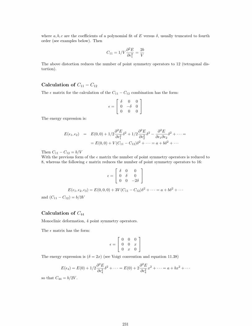
where a, b, c are the coefficients of a polynomial fit of E versus δ, usually truncated to fourthorder (see examples below). Then

C11 = 1/V∂2E

∂ε21=

2bV

The above distortion reduces the number of point symmetry operators to 12 (tetragonal dis-tortion).

Calculation of C11 − C12

The ε matrix for the calculation of the C11 − C12 combination has the form:

ε =

δ 0 00 −δ 00 0 0

The energy expression is:

E(ε1, ε2) = E(0, 0) + 1/2∂2E

∂ε21δ2 + 1/2

∂2E

∂ε22δ2 − ∂2E

∂ε1∂ε2δ2 + · · · =

= E(0, 0) + V (C11 − C12)δ2 + · · · = a+ bδ2 + · · ·

Then C11 − C12 = b/VWith the previous form of the ε matrix the number of point symmetry operators is reduced to8, whereas the following ε matrix reduces the number of point symmetry operators to 16:

ε =

δ 0 00 δ 00 0 −2δ

E(ε1, ε2, ε3) = E(0, 0, 0) + 3V (C11 − C12)δ2 + · · · = a+ bδ2 + · · ·

and (C11 − C12) = b/3V

Calculation of C44

Monoclinic deformation, 4 point symmetry operators.

The ε matrix has the form:

ε =

0 0 00 0 x0 x 0

The energy expression is (δ = 2x) (see Voigt convention and equation 11.38)

E(ε4) = E(0) + 1/2∂2E

∂ε24δ2 + · · · = E(0) + 2

∂2E

∂ε24x2 + · · · = a+ bx2 + · · ·

so that C44 = b/2V .

231

Calculation of C44

Rhombohedral deformation, 12 point symmetry operators.


ε =

0 x xx 0 xx x 0

The energy expression is (δ = 2x,C45 = C46 = C56 = 0)

E(ε4, ε5, ε6) = E(0) + 3/2∂2E

∂ε24δ2 + · · · = E(0) + 6

∂2E

∂ε24x2 + · · · = a+ bx2 + · · ·

so that C44 = b/6V .

Bulk modulus

The bulk modulus can be evaluated simply by varying the lattice constant, (1 in cubic systems)without the use of the ε matrix, and fitting the curve E(V ).If the ε matrix is used, the relation between B and Cij (cubic systems) must be taken intoaccount:

B = (C11 + 2C12)/3


ε =

δ 0 00 δ 00 0 δ

and the energy:

E(ε) = E(0) + 3/2∂2E

∂ε21δ2 + 3

∂2E

∂ε1∂ε2δ2 = (11.39)

= E(0) +3V2

[C11 + 2C12]δ2 (11.40)

so that B = 29V b

N.B. Conversion factors:1 hartree A−3 = 4359.74812 GPa1 GPa = 1 GN m−2 = 1 GJ m−3 = 1010 dyne cm−2 = 10−2 Mbar.

232

11.10 Spontaneous polarization through the Berry phaseapproach

The electronic phase of a system λ in the direction 1, ϕ(λ,1)el , can be written as:

ϕ(λ,1)el =

1s2s3

∑j2,j3

∑j1

∆ϕ(λ,1)j1,j2,j3

(k) (11.41)

The electronic contribution to the polarization of a system λ can be written as :

P(λ)el =

1Ω(λ)

(B(λ)

)−1

ϕ(λ)el (11.42)

Where (B(λ))−1 is the reciprocal lattice vectors components inverse matrix and ϕ(λ)el the elec-

tronic phase difference vector of a system λ (which components are ϕ(λ,i)el ). The nuclear con-

tribution to the polarization of a system λ, P(λ)nuc can also be written as:

P(λ)nuc =

1Ω(λ)

∑A

R(λ)A · ZA (11.43)

where R(λ)A and ZA are the position vector and the nuclear charge of the atom A respectively of

the system λ. The total polarization is the sum of these two contributions and can be writtenas

P(λ)tot = P(λ)

nuc + P(λ)el (11.44)

The spontaneous polarization is the difference between the systems λ = 1 and λ = 0

P = P(λ)tot −P(λ)

tot (11.45)

Spontaneous polarization through the localized crystallineorbitals approach

The electronic contribution to the polarization of a system λ, P(λ)el , can be written as

P(λ)el =

e

Ω(λ)

∑µ

〈rµ〉 (11.46)

Where 〈rµ〉 is the centroid of the Wannier function µ.The nuclear contribution to the polarization of a system λ, P(λ)

nuc can also be written as

P(λ)nuc =

1Ω(λ)

∑A

RA · ZA (11.47)

where RA and ZA are the position vector and the nuclear charge of the atom A respectively.The total polarization is the sum of these two contributions and can be written as

P(λ)tot = P(λ)

nuc + P(λ)el (11.48)

The spontaneous polarization is the difference between the both systems λ = 1 and λ = 0:

P = P(1)tot −P(2)

tot (11.49)

To calculate the spontaneous polarization, a preliminary run is needed for each of the twosystems λ = 1 and λ = 0. Then a third run with the keyword SPOLWF gives the difference ofpolarization between systems λ = 1 and λ = 0.

233

11.11 Piezoelectricity through the Berry phase approach

The electronic phase vector of a system λ, is given by (2.1). The nuclear phase vector of asystem λ, ϕ(λ)

nuc, can be written as

ϕ(λ)nuc = Ω(λ) B(λ)P(λ)

nuc (11.50)

Where B(λ) reciprocal lattice vectors components matrix.The last equation can be simplifiedthanks to (11.43):

ϕ(λ)nuc = B(λ)

∑A

R(λ)A · ZA (11.51)

So the phase vector of a system λ, ϕ(λ) is:

ϕ(λ) = ϕ(λ)nuc + ϕ

(λ)el (11.52)

The proper piezoelectric constants can be obtained by:

eijk = − 12π

1Ω

∑α

dϕα

dεjkaα,i (11.53)

Where ϕα is projection of the phase ϕ along the α direction and aα,i is the component of alattice vector aα along the cartesian axis i . To obtain the improper piezoelectric constants,the following correction must done:

eijk = eijk + δijPk − δjkPi (11.54)

In the piezoelectric constants calculations the dϕα

dεjkterm is evaluated numerically. The calcu-

lated term is:dϕα

dεjk' ∆ϕα

∆εjk=ϕ

(1)α − ϕ

(0)α

ε(1)jk − ε

(0)jk

(11.55)

Piezoelectricity through the localized crystalline orbitalsapproach

The electronic phase vector of a system λ, is given by:

ϕ(λ)el = Ω(λ) B(λ)P(λ)

el (11.56)

Where B(λ) reciprocal lattice vectors components matrix. The nuclear phase vector of a systemλ, ϕ(λ)

nuc, can be written asϕ(λ)

nuc = Ω(λ) B(λ)P(λ)nuc (11.57)

The last equation can be simplified thanks to 11.43:

ϕ(λ)nuc = B(λ)

∑A

R(λ)A · ZA (11.58)

So the phase vector of a system λ, ϕ(λ) is:

ϕ(λ) = ϕ(λ)nuc + ϕ

(λ)el (11.59)

The proper piezoelectric constants can be obtained by:

eijk = − 12π

1Ω

∑α

dϕα

dεjkaα,i (11.60)

Where ϕα is projection of the phase ϕ along the α direction and aα,i is the component of alattice vector aα along the cartesian axis i . To obtain the improper piezoelectric constants,the following correction must done:

eijk = eijk + δijPk − δjkPi (11.61)

234

In the piezoelectric constants calculations the dϕα

dεjkterm is evaluated numerically. The calcu-

lated term is:dϕα

dεjk' ∆ϕα

∆εjk=ϕ

(1)α − ϕ

(0)α

ε(1)jk − ε

(0)jk

(11.62)

235

Appendix A

Symmetry groups

A.1 Labels and symbols of the space groups

The labels are according to the International Tables for Crystallography [64]. The symbols arederived by the standard SHORT symbols, as shown in the following examples:

Symbol Input to CRYSTALP 6 2 m → P -6 2 M ;P 63 m → P 63 M.

For the groups 221-230 the symbols are according to the 1952 edition of the InternationalTables, not to the 1982 edition. The difference involves the 3 axis: 3 (1952 edition); 3 (1982edition) (Example group 221: 1952 ed. → P m 3 m ; 1982 ed. → P m 3 m)

236

IGR symbol

Triclinic lattices1 P12 P 1

Monoclinic lattices3 P24 P21

5 C26 Pm7 Pc8 Cm9 Cc10 P2/m11 P21/m12 C2/m13 P2/c14 P21/c15 C2/c

Orthorhombic lattices16 P22217 P2221

18 P2121219 P212121

20 C2221

21 C22222 F22223 I22224 I212121

25 Pmm226 Pmc21

27 Pcc228 Pma229 Pca21

30 Pnc231 Pmn21

32 Pba233 Pna21

34 Pnn235 Cmm236 Cmc21

IGR symbol

37 Ccc238 Amm239 Abm240 Ama241 Aba242 Fmm243 Fdd244 Imm245 Iba246 Ima247 Pmmm48 Pnnn49 Pccm50 Pban51 Pmma52 Pnna53 Pmna54 Pcca55 Pbam56 Pccn57 Pbcm58 Pnnm59 Pmmn60 Pbcn61 Pbca62 Pnma63 Cmcm64 Cmca65 Cmmm66 Cccm67 Cmma68 Ccca69 Fmmm70 Fddd71 Immm72 Ibam73 Ibca74 Imma

IGR symbol

Tetragonal lattices75 P476 P41

77 P42

78 P43

79 I480 I41

81 P 482 I 483 P4/m84 P42/m85 P4/n86 P42/n87 I4/m88 I41/a89 P42290 P421291 P412292 P4121293 P422294 P4221295 P432296 P4321297 I42298 I412299 P4mm100 P4bm101 P42cm102 P42nm103 P4cc104 P4nc105 P42mc106 P42bc107 I4mm108 I4cm109 I41md110 I41cd111 P 42m112 P 42c

237

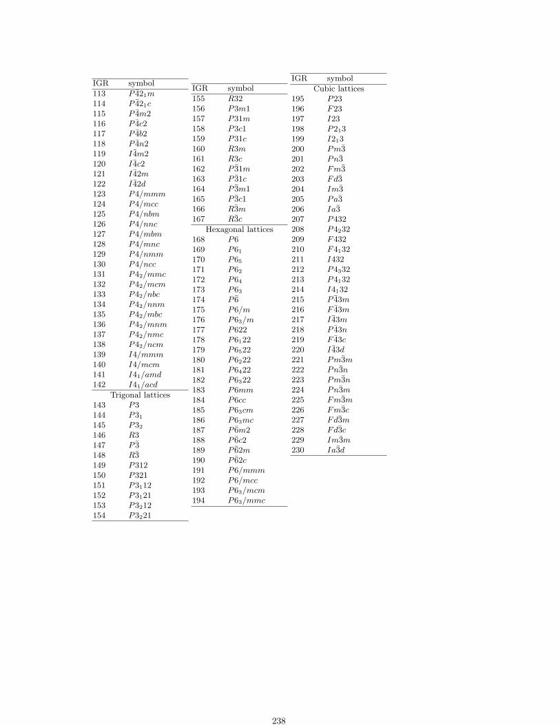
IGR symbol

113 P 421m114 P 421c115 P 4m2116 P 4c2117 P 4b2118 P 4n2119 I 4m2120 I 4c2121 I 42m122 I 42d123 P4/mmm124 P4/mcc125 P4/nbm126 P4/nnc127 P4/mbm128 P4/mnc129 P4/nmm130 P4/ncc131 P42/mmc132 P42/mcm133 P42/nbc134 P42/nnm135 P42/mbc136 P42/mnm137 P42/nmc138 P42/ncm139 I4/mmm140 I4/mcm141 I41/amd142 I41/acd

Trigonal lattices143 P3144 P31

145 P32

146 R3147 P 3148 R3149 P312150 P321151 P3112152 P3121153 P3212154 P3221

IGR symbol

155 R32156 P3m1157 P31m158 P3c1159 P31c160 R3m161 R3c162 P 31m163 P 31c164 P 3m1165 P 3c1166 R3m167 R3c

Hexagonal lattices168 P6169 P61

170 P65

171 P62

172 P64

173 P63

174 P 6175 P6/m176 P63/m177 P622178 P6122179 P6522180 P6222181 P6422182 P6322183 P6mm184 P6cc185 P63cm186 P63mc187 P 6m2188 P 6c2189 P 62m190 P 62c191 P6/mmm192 P6/mcc193 P63/mcm194 P63/mmc

IGR symbol

Cubic lattices195 P23196 F23197 I23198 P213199 I213200 Pm3201 Pn3202 Fm3203 Fd3204 Im3205 Pa3206 Ia3207 P432208 P4232209 F432210 F4132211 I432212 P4332213 P4132214 I4132215 P 43m216 F 43m217 I 43m218 P 43n219 F 43c220 I 43d221 Pm3m222 Pn3n223 Pm3n224 Pn3m225 Fm3m226 Fm3c227 Fd3m228 Fd3c229 Im3m230 Ia3d

238

A.2 Labels of the layer groups (slabs)

The available layer groups belong to a subset of the 230 space groups. Therefore they can beidentified by the corresponding space group.The first column gives the label to be used in the input card (IGR variable).The second column gives the Hermann-Mauguin symbol of the corresponding space group(generally the short one; the full symbol is adopted when the same short symbol could referto different settings). The third column gives the Schoenflies symbol. The fourth column thenumber of the corresponding space group, according to the International Tables for Crystal-lography. The number of the space group is written in parentheses when the orientation of thesymmetry operators does not correspond to the first setting in the I. T.

IGR HermannMauguin

Schoenflies N

Oblique lattices (P)1 P1 C1

1 12 P 1 C1

i 23 P112 C1

2 (3)4 P11m C1

s (6)5 P11a C2

s (7)6 P112/m C1

2h (10)7 P112/a C4

2h (13)

Rectangular lattices (P or C)8 P211 C1

2 (3)9 P2111 C2

2 (4)10 C211 C3

2 (5)11 Pm11 C1

s (6)12 Pb11 C2

s (7)13 Cm11 C3

s (8)14 P2/m11 C1

2h (10)15 P21/m11 C2

2h (11)16 C2/m11 C3

2h (12)17 P2/b11 C4

2h (13)18 P2/b11 C5

2h (14)19 P222 D1

2 1620 P2212 D2

2 (17)21 P21212 D3

2 1822 C222 D6

2 2123 Pmm2 C1

2v 2524 Pma2 C4

2v 2825 Pba2 C8

2v 3226 Cmm2 C1

2v 3527 P2mm C1

2v (25)28 P21am C2

2v (26)29 P21ma C2

2v (26)30 P2mb C4

2v (28)31 P21mn C7

2v (31)32 P2aa C3

2v (27)33 P21ab C5

2v (29)34 P2an C6

2v (30)35 C2mm C1

2v (38)36 C2mb C5

2v (39)37 Pmmm D1

2h 4738 Pmam D5

2h (51)39 Pmma D5

2h 5140 Pmmn D3

2h 59

IGR HermannMauguin

Schoenflies N

41 Pbam D92h 55

42 Pmaa D32h (49)

43 Pman D72h (53)

44 Pbma D12h (57)

45 Pbaa D82h (54)

46 Pban D42h 50

47 Cmmm D92h 65

48 Cmma D22h 67

Square lattices (P)49 P4 C1

4 7550 P 4 S1

4 8151 P4/m C1

4h 8352 P4/n C3

4h 8553 P422 D1

4 8954 P4212 D2

4 9055 P4mm C1

4v 9956 P4bm C2

4v 10057 P 42m D1

2d 11158 P 421m D3

2d 11359 P 4m2 D5

2d 11560 P 4b2 D7

2d 11761 P4/mmm D1

4h 12362 P4/nbm D3

4h 12563 P4/mbm D5

4h 12764 P4/nmm D7

4h 129

Hexagonal lattices (P)65 P3 C1

3 14366 P 3 C1

3i 14767 P312 D1

3 14968 P321 D2

3 15069 P3m1 C1

3v 15670 P31m C2

3v 15771 P 31m D1

3d 16272 P 3m1 D3

3d 16473 P6 C1

6 16874 P 6 C1

3h 17475 P6/m C1

6h 17576 P622 D1

6 17777 P6mm C1

6v 18378 P 6m2 D1

3h 18779 P 62m D3

3h 18980 P6/mmm D1

6h 191

239

A.3 Labels of the rod groups (polymers)

The available rod groups belong to a subset of the 230 space groups; the symmetry operatorsare generated for the space groups (principal axis z) and then rotated by 90 through y, tohave the polymer axis along x (CRYSTAL convention).In the table, the first column gives the label to be used in the input card for identifying therod group (IGR variable).The second column gives the ”polymer” symbol, according to the the following convention: xis the first symmetry direction, y the second.The third column gives the Schoenflies symbol.The fourth column gives the Hermann-Mauguin symbol (generally the short one; the full symbolis adopted when the same short symbol could refer to different settings) of the correspondingspace group (principal axis z).The fifth column gives the number of the corresponding space group, according to the Interna-tional Tables for Crystallography; this number is written in parentheses when the orientationof the symmetry operators does not correspond to the first setting in the I. T.

”Polymer” Hermann Number ofIGR symbol Schoenflies Mauguin space group

(x direction) (z direction)

1 P1 C11 P1 1

2 P 1 C1i P 1 2

3 P211 C12 P112 (3)

4 P2111 C22 P1121 (4)

5 P121 C12 P121 (3)

6 P112 C12 P211 (3)

7 Pm11 C1s P11m (6)

8 P1m1 C1s P1m1 (6)

9 P1a1 C2s P1c1 (7)

10 P11m C1s Pm11 (6)

11 P11a C2s Pc11 (7)

12 P2/m11 C12h P112/m (10)

13 P21/m11 C22h P1121/m (11)

14 P12/m1 C12h P12/m1 (10)

15 P12/a1 C42h P12/c1 (13)

16 P112/m C12h P2/m11 (10)

17 P112/a C42h P2/c11 (13)

18 P222 D12 P222 16

19 P2122 D22 P2221 17

20 P2mm C12v Pmm2 25

21 P21am C22v Pmc21 26

22 P21ma C22v Pcm21 (26)

23 P2aa C32v Pcc2 27

24 Pm2m C12v Pm2m (25)

25 Pm2a C42v Pc2m (28)

26 Pmm2 C12v P2mm (25)

27 Pma2 C42v P2cm (28)

28 Pmmm D12h Pmmm 47

29 P2/m2/a2/a D32h Pccm 49

30 P21/m2/m2/a D52h Pcmm (51)

31 P21/m2/a2/m D52h Pmcm (51)

240



32 P4 C14 P4 75

33 P41 C24 P41 76

34 P42 C34 P42 77

35 P43 C44 P43 78

36 P 4 S14 P 4 81

37 P4/m C14h P4/m 83

38 P42/m C24h P42/m 84

39 P422 D14 P422 89

40 P4122 D34 P4122 91

41 P4222 D54 P4222 93

42 P4322 D74 P4322 95

43 P4mm C14v P4mm 99

44 P42am C34v P42cm 101

45 P4aa C54v P4cc 103

46 P42ma C74v P42mc 105

47 P 42m D12d P 42m 111

48 P 42a D22d P 42c 112

49 P 4m2 D52d P 4m2 115

50 P 4a2 D62d P 4c2 116

51 P4/mmm D14h P4/mmm 123

52 P4/m2/a2/a D24h P4/mcc 124

53 P42/m2/m2/a D94h P42/mmc 131

54 P42/m2/a2/m D104h P42/mcm 132

55 P3 C13 P3 143

56 P31 C23 P31 144

57 P32 C33 P32 145

58 P 3 C13i P 3 147

59 P312 D13 P312 149

60 P3112 D33 P3112 151

61 P3212 D53 P3212 153

62 P321 D23 P321 150

63 P3121 D43 P3121 152

64 P3221 D63 P3221 154

65 P3m1 C13v P3m1 156

66 P3a1 C33v P3c1 158

67 P31m C23v P31m 157

68 P31a C43v P31c 159

69 P 31m D13d P 31m 162

70 P 31a D23d P 31c 163

71 P 3m1 D33d P 3m1 164

72 P 3a1 D43d P 3c1 165

241



73 P6 C16 P6 168

74 P61 C26 P61 169

75 P65 C36 P65 170

76 P62 C46 P62 171

77 P64 C56 P64 172

78 P63 C66 P66 173

79 P 6 C13h P 6 174

80 P6/m C16h P6/m 175

81 P63/m C26h P63/m 176

82 P622 D16 P622 177

83 P6122 D26 P6122 178

84 P6522 D36 P6522 179

85 P6222 D46 P6222 180

86 P6422 D56 P6422 181

87 P6322 D66 P6322 182

88 P6mm C16v P6mm 183

89 P6aa C26v P6cc 184

90 P63am C36v P63cm 185

91 P63ma C46v P63mc 186

92 P 6m2 D13h P 6m2 187

93 P 6a2 D23h P 6c2 188

94 P 62m D33h P 62m 189

95 P 62a D43h P 62c 190

96 P6/mmm D16h P6/mmm 191

97 P6/m2/a2/a D26h P6/mcc 192

98 P63/m2/a2/m D36h P63/mcm 193

99 P63/m2/m2/a D46h P63/mmc 194

242

A.4 Labels of the point groups (molecules)

The centre of symmetry is supposed to be at the origin; for the rotation groups the principalaxis is z.The first column gives the label to be used in the input card for identifying the point group(IGR variable). The second column gives the short Hermann-Mauguin symbol. The thirdcolumn gives the Schoenflies symbol; for the C2 , C2h and Cs groups the C2 direction or thedirection orthogonal to the plane is indicated. The fourth column gives the number of purerotations for molecules (σ).

IGR Hermann Schoenflies σMauguin

1 1 C1 12 1 Ci 13 2 (x) C2 (x) 24 2 (y) C2 (y) 25 2 (z) C2 (z) 26 m (x) Cs (x) 17 m (y) Cs (y) 18 m (z) Cs (z) 19 2/m (x) C2h (x) 210 2/m (y) C2h (y) 211 2/m (z) C2h (z) 212 222 D2 413 2mm C2v (x) 214 m2m C2v (y) 215 mm2 C2v (z) 216 mmm D2h 417 4 C4 418 4 S4 219 4/m C4h 420 422 D4 821 4mm C4v 422 42m D2d (σv planes along x+y and x-y) 423 4m2 D2d (σv planes along x and y) 424 4/mmm D4h 825 3 C3 326 3 C3i 327 321 D3 (one C2 axis along y) 628 312 D3 (one C2 axis along x) 629 3m1 C3v (one σv plane along x) 330 31m C3v (one σv plane along y) 331 3m1 D3d (one σd plane along x) 632 31m D3d (one σd plane along y) 633 6 C6 634 6 C3h 335 6/m C6h 636 622 D6 1237 6mm C6v 638 6m2 D3h (one C2 axis along x) 639 62m D3h (one C2 axis along y) 640 6/mmm D6h 1241 23 T 1242 m3 Th 1243 432 O 2444 43m Td 1245 m3m Oh 24

243

A.5 From conventional to primitive cells:transforming matrices

The matrices describing the transformations from conventional (given as input) to primitive(internally used by CRYSTAL) cells of Bravais lattices are coded in CRYSTAL. A point called xin the direct lattice has xP coordinates in a primitive cell and xC coordinates in a conventionalcell. The relation between xP and xC is the following:

WxP = xC (A.1)

Likewise, for a point in the reciprocal space the following equation holds:

W−1x∗P = x∗C (A.2)

The W transforming matrices adopted in CRYSTAL, and reported below, satisfy the followingrelation between the two metric tensors GP and GC :

GP = WGCW (A.3)

The values of the elements of the metric tensors GP and GC agree with those displayed inTable 5.1 of the International Tables of Crystallography (1992 edition).

P → A

0BBBB@1 0 0

0 12

12

0 12

12

1CCCCA P → B

0BBBB@12

0 12

0 1 0

12

0 12

1CCCCA

P → C

0BBBB@12

12

0

12

12

0

0 0 1

1CCCCA P → F

0BBBB@0 1

212

12

0 12

12

12

0

1CCCCA

P → I

0BBBB@12

12

12

12

12

12

12

12

12

1CCCCA R→ H

0BBBB@23

13

13

13

13

23

13

13

13

1CCCCA

A→ P

0@ 1 0 00 1 10 −1 1

1A B → P

0@ 1 0 −10 1 01 0 1

1A

C → P

0@ 1 1 0−1 1 0

0 0 1

1A F → P

0@ −1 1 11 −1 11 1 −1

1A

I → P

0@ 0 1 11 0 11 1 0

1A H → R

0@ 1 0 1−1 1 1

0 −1 1

1A

Table A.1: W matrices for the transformation from conventional to primitive and from prim-itive to conventional cells. P stands for primitive, A, B and C for A-, B- and C-face centred,I for body centred, F for all-face centred, R for primitive rhombohedral (‘rhombohedral axes’)and H for rhombohedrally centred (‘hexagonal axes’) cell (Table 5.1, ref. [64]).

244

Appendix B

Summary of input keywords

All the keywords are entered with an A format; the keywords must be typed left-justified, withno leading blanks. The input is not case sensitive.

Geometry (Input block 1)

Symmetry information

ATOMSYMM printing of point symmetry at the atomic positions 34 –MAKESAED printing of symmetry allowed elastic distortions (SAED) 45 –PRSYMDIR printing of displacement directions allowed by symmetry. 53 –SYMMDIR printing of symmetry allowed geom opt directions 60 –SYMMOPS printing of point symmetry operators 60 –TENSOR print tensor of physical properties up to order 4 60 I

Symmetry information and control

BREAKELAS symmetry breaking according to a general distortion 35 IBREAKSYM allow symmetry reduction following geometry modifications 34 –KEEPSYMM maintain symmetry following geometry modifications 44 –MODISYMM removal of selected symmetry operators 45 IPURIFY cleans atomic positions so that they are fully consistent with the

group53 –

SYMMREMO removal of all symmetry operators 60 –TRASREMO removal of symmetry operators with translational components 60 –

Modifications without reduction of symmetry

ATOMORDE reordering of atoms in molecular crystals 32 –NOSHIFT no shift of the origin to minimize the number of symmops with

translational components before generating supercell52 –

ORIGIN shift of the origin to minimize the number of symmetry operatorswith translational components

52 –

PRIMITIV crystallographic cell forced to be the primitive cell 52 –ROTCRY rotation of the crystal with respect to the reference system cell 54 I

Atoms and cell manipulation (possible symmetry reduction (BREAKSYMM)

245

ATOMDISP displacement of atoms 32 IATOMINSE addition of atoms 32 IATOMREMO removal of atoms 32 IATOMROT rotation of groups of atoms 33 IATOMSUBS substitution of atoms 34 IELASTIC distortion of the lattice 38 IPOINTCHG point charges input 52 ISCELPHONO generation of supercell for phonon dispersion 58 ISUPERCEL generation of supercell - input refers to primitive cell 56 ISUPERCON generation of supercell - input refers to conventional cell 56 IUSESAED given symmetry allowed elastic distortions, reads δ 61 I

From crystals to slabs (3D→2D)

SLABINFO definition of a new cell, with xy ‖ to a given plane 56 ISLABCUT generation of a slab parallel to a given plane (3D→2D) 55 I

From slabs to nanotubes (2D→1D)

NANOTUBE building a nanotube from a slab 47 ISWCNT building a nanotube from an hexagonal slab 50 I

From periodic structure to clusters

CLUSTER cutting of a cluster from a periodic structure (3D→0D) 36 IHYDROSUB border atoms substituted with hydrogens (0D→0D) 44 I

Molecular crystals

MOLECULE extraction of a set of molecules from a molecular crystal(3D→0D)

46 I

MOLEXP variation of lattice parameters at constant symmetry and molec-ular geometry (3D→3D)

46 I

MOLSPLIT periodic structure of non interacting molecules (3D→3D) 47 –RAYCOV modification of atomic covalent radii 53 I

BSSE correction

MOLEBSSE counterpoise method for molecules (molecular crystals only)(3D→0D)

45 I

ATOMBSSE counterpoise method for atoms (3D→0D) 31 I


ANGSTROM sets input units to Angstrom 31 –BOHR sets input units to bohr 34 –BOHRANGS input bohr to A conversion factor (0.5291772083 default value) 34 IBOHRCR98 bohr to A conversion factor is set to 0.529177 (CRY98 value) –END/ENDG terminate processing of geometry input –FRACTION sets input units to fractional 44 –NEIGHBOR number of neighbours in geometry analysis 51 IPARAMPRT printing of parameters (dimensions of static allocation arrays) 52 –PRINTCHG printing of point charges coordinates in geometry output 52PRINTOUT setting of printing options by keywords 53 –SETINF setting of inf array options 54 ISETPRINT setting of printing options 54 ISTOP execution stops immediately 56 –TESTGEOM stop after checking the geometry input 60 –


246

COORPRT coordinates of all the atoms in the cell 37 –EXTPRT write file in CRYSTAL geometry input format 41 –FINDSYM write file in FINDSYM input format 44 –STRUCPRT cell parameters and coordinates of all the atoms in the cell 56 –

External electric field - modified Hamiltonian

FIELD electric field applied along a periodic direction 41 IFIELDCON electric field applied along a non periodic direction 43 I

Geometry optimization - see index for keywords full list

OPTGEOM Geometry optimization input block - closed by END 105 IType of optimization (default: atom coordinates)FULLOPTG full geometry optimization –CELLONLY cell parameters optimization –INTREDUN optimization in redundant internal coordinates 115 –ITATOCEL iterative optimization (atom/cell) –CVOLOPT full geometry optimization at constant volume 117 –Initial HessianHESSIDEN initial guess for the Hessian - identity matrix –HESSMOD1 initial guess for the Hessian - model 1 (default) –HESSMOD2 initial guess for the Hessian - model 2 –HESSNUM initial guess for the Hessian - numerical estimate –Convergence criteria modificationTOLDEG RMS of the gradient [0.0003] ITOLDEX RMS of the displacement [0.0012] ITOLDEE energy difference between two steps [10−7] IMAXCYCLE max number of optimization steps IOptimization controlFRAGMENT partial geometry optimization 119 IRESTART data from previous run –FINALRUN Wf single point with optimized geometry IGradient calculation controlNUMGRATO numerical atoms first derivatives 114 –NUMGRCEL numerical cell first derivatives 114 –NUMGRALL numerical atoms and cell first derivatives 114 –External stressEXTSTRESS apply external stress 121 IEXTPRESS apply external hydrostatic pressure 121 IPrinting optionsPRINTFORCES atomic gradients –PRINTHESS Hessian –PRINTOPT optimization procedure –PRINT verbose printing –

Frequencies at Γ - Harmonic calculation

247

FREQCALC Frequencies at Γ (harmonic calculation) input block - closed by END 127 IANALYSIS –[NOANALYSIS] –DIELISO IDIELTENS IEND[FREQ] –FRAGMENT IINTENS –INTLOC - IR intensities through Wannier functions 134 –[INTPOL] - IR intensities through Berry phase [default] 134 –ISOTOPES 129 I[MODES] –[NOINTENS] –NOMODES –NORMBORN –NOUSESYMM –NUMDERIV IPRESSURE IPRINT –RESTART –SCANMODE ISTEPSIZE ITEMPERAT ITESTFREQ –[USESYMM] –

ANHARM Frequency at Γ (anharmonic calculationinput block - closed by END142 IEND[ANHA] –ISOTOPES modification of atomic mass 143 IKEEPSYMM 44 –NOGUESS 143 –POINTS26 143 –PRINT –TEST[ANHA] –

CONFCNT - Configuration counting and cluster expansion 147

CPHF - Coupled Perturbed Hartree-Fock 145

ELASTCON - Second order elastic constants 149

EOS - Equation of state 145

Basis set input (Input block 2)

Symmetry control

ATOMSYMM printing of point symmetry at the atomic positions 34 –

Basis set modification

248

CHEMOD modification of the electronic configuration 62 IGHOSTS eliminates nuclei and electrons, leaving BS 64 I


CHARGED allows non-neutral cell 62 –NOPRINT printing of basis set removed 64 –PARAMPRT printing of parameters controlling code dimensions 52 –PRINTOUT setting of printing options 53 ISETINF setting of inf array options 54 ISETPRINT setting of printing options 54 ISTOP execution stops immediately 56 –SYMMOPS printing of point symmetry operators 60 –END/ENDB terminate processing of basis set definition keywords –


GAUSS98 printing of an input file for the GAUSS94/98 package 64 –

General information, hamiltonian, SCF (Input block 3)

All DFT related keyword are collected under the heading ”DFT”, closed b END[DFT]

Single particle Hamiltonian

RHF Restricted Closed Shell 96 –UHF Unrestricted Open Shell 102 –

249

DFT DFT Hamiltonian 102 –SPIN spin-polarized solution 75 –Choice of the exchange-correlation functionalsCORRELAT correlation functional 74 I

LYP Lee-Yang-Parr [78] (GGA)P86 Perdew 86 [88] (LDA)PBE Perdew-Becke-Ernzerhof [90] (GGA)PBESOL GGA. PBE functional revised for solids [96]PWGGA Perdew-Wang 91 (GGA)PWLSD Perdew-Wang 92 [92, 93, 91] (GGA)PZ Perdew-Zunger [94] (LDA)VBH von Barth-Hedin [127] (LDA)WL GGA - Wilson-Levy [133]VWN Vosko,-Wilk-Nusair [128] (LDA)

EXCHANGE exchange functional 75 IBECKE Becke [13] (GGA)LDA Dirac-Slater [34] (LDA)PBE Perdew-Becke-Ernzerhof [90] (GGA)PBESOL GGA. PBE functional revised for solids [96]PWGGA Perdew-Wang 91 (GGA)SOGGA second order GGA. [136]VBH von Barth-Hedin [127] (LDA)WCGGA GGA - Wu-Cohen [135]

Global keywords: exchange+correlationB3PW B3PW parameterization 76 –B3LYP B3LYP parameterization 76 –PBE0 Adamo and Barone [2] 76SOGGAXC see [136] 76Custom made dft exchange-local exchangeHYBRID hybrid mixing 76 INONLOCAL local term parameterization 76 INumerical accuracy controlANGULAR definition of angular grid IBATCHPNT grid point grouping for integration I[BECKE] selection of Becke weights (default) –[CHUNKS] max n. points in a batch for numerical int. ILGRID ”large” predefined grid IRADSAFE safety radius for grid point screening IRADIAL definition of radial grid ISAVIN selection of Savin weights –TOLLDENS density contribution screening 6 ITOLLGRID grid points screening 14 IXLGRID ”extra large” predefined grid IXXLGRID ”extra extra large” predefined grid IAtomic parameters controlRADIUS customized atomic radius 81 IFCHARGE customized formal atomic charge 81 IAuxiliaryPRINT extended printingEND close DFT input block

Numerical accuracy and computational parameters control

250

BIPOLAR Bipolar expansion of bielectronic integrals 73 IBIPOSIZE size of coulomb bipolar expansion buffer 73 IEXCHSIZE size of exchange bipolar expansion buffer 73 IINTGPACK Choice of integrals package 0 92 INOBIPCOU Coulomb bielectronic integrals computed exactly 95 –NOBIPEXCH Exchange bielectronic integrals computed exactly 95 –NOBIPOLA All bielectronic integrals computed exactly 95 –POLEORDR Maximum order of multipolar expansion 4 96 ITOLINTEG Truncation criteria for bielectronic integrals 6 6 6 6 12 102 ITOLPSEUD Pseudopotential tolerance 6 102 I

Type of executionMPP MPP execution 93

Type of run

ATOMHF Atomic wave functions 72 ISCFDIR SCF direct (mono+biel int computed) 96 –EIGS S(k) eigenvalues - basis set linear dependence check 81 –FIXINDEX Reference geometry to classify integrals 86 –

Basis set - AO occupancy

FDAOSYM f and d degeneracies analysis 83 IFDAOCCUP f and d orbital occupation guess 84 IGUESDUAL Density matrix guess - different Basis set 89 I

Integral file distribution

BIESPLIT writing of bielectronic integrals in n files n = 1 ,max=10 73 IMONSPLIT writing of mono-electronic integrals in n file n = 1 , max=10 93 I

Numerical accuracy control and convergence tools

ANDERSON Fock matrix mixing 71 IBROYDEN Fock matrix mixing 73 IFMIXING Fock/KS matrix (cycle i and i-1) mixing 0 87 ILEVSHIFT level shifter no 92 IMAXCYCLE maximum number of cycles 50 93 ISMEAR Finite temperature smearing of the Fermi surface no 99 ITOLDEE convergence on total energy 5 102 ITOLDEP convergence on density matrix 16 102 I

Initial guess

EIGSHIFT alteration of orbital occupation before SCF no 82 IEIGSHROT rotation of the reference frame no 82 IGUESSP density matrix from a previous run 91 –GUESSPAT superposition of atomic densities 91 –


ATOMSPIN setting of atomic spin to compute atomic densities 72 IBETALOCK beta electrons locking 73 ISPINLOCK spin difference locking 101 ISPINEDIT editing of the spin density matrix used as SCF guess 100 I


251

END terminate processing of block3 input –KSYMMPRT printing of Bloch functions symmetry analysis 92 –NEIGHBOR number of neighbours to analyse in PPAN 51 IPARAMPRT output of parameters controlling code dimensions 52 –PRINTOUT setting of printing options 53 INOSYMADA No Symmetry Adapted Bloch Functions 95 –SYMADAPT Symmetry Adapted Bloch Functions (default) 101 –SETINF setting of inf array options 54 ISETPRINT setting of printing options 54 ISTOP execution stops immediately 56 –TESTPDIM stop after symmetry analysis 101 –TEST[RUN] stop after integrals classification and disk storage estimate 101 –


NOFMWF wave function formatted output not written in file fort.98. 95 –SAVEWF wave function data written every two SCF cycles 97 –

Post SCF calculations

POSTSCF post-scf calculations when convergence criteria not satisfied 96 –EXCHGENE exchange energy evaluation (spin polarized only) 83 –GRADCAL analytical gradient of the energy 87 –PPAN population analysis at the end of the SCF no 96

Properties

RDFMWF wave function data conversion formatted-binary (fort.98 → fort.9)

Preliminary calculations

NEWK Eigenvectors calculation 179 INOSYMADA No symmetry Adapted Bloch Functions 95 –PATO Density matrix as superposition of atomic (ionic) densities 180 IPBAN Band(s) projected density matrix (preliminary NEWK) 180 IPGEOMW Density matrix from geometrical weights (preliminary NEWK) 181 IPDIDE Energy range projected density matrix (preliminary NEWK) 181 IPSCF Restore SCF density matrix 187 –

Properties computed from the density matrix

ADFT Atomic density functional correlation energy 155 IBAND Band structure 157 IBIDIERD Reciprocal form factors 158 ICLAS Electrostatic potential maps (point multipoles approximation) 159 IECHG Charge density and charge density gradient - 2D grid 164 IECH3 Charge density - 3D grid 163 IEDFT Density functional correlation energy (HF wave function only) 164 IEMDLPG Electron momentum distribution from density matrix 166 IPMP2 MP2 correction to the Valence Density Matrix 181POLI Atom and shell multipoles evaluation 182 IPOTM Electrostatic potential - 2D grid 185 IPOT3 Electrostatic potential - 3D grid 183 IPOTC Electrostatic properties 184 IPPAN Mulliken population analysis 96XFAC X-ray structure factors 188 I

Properties computed from the density matrix (spin-polarized systems)

252

ANISOTRO Hyperfine electron-nuclear spin tensor 156 IISOTROPIC Hyperfine electron-nuclear spin interaction - Fermi contact 168 IPOLSPIN Atomic spin density multipoles 182 I

Properties computed from eigenvectors (after keyword NEWK)

ANBD Printing of principal AO component of selected CO 155 IBWIDTH Printing of bandwidth 159 IDOSS Density of states 162 IEMDL Electron momentum distribution - line 165 IEMDP Electron momentum distribution - plane maps 166 IPROF Compton profiles and related quantities 186 I

New properties

POLARI Berry phase calculations 190 ISPOLBP Spontaneous polarization (Berry phase approach) 192 –SPOLWF Spontaneous polarization (localized CO approach) 193 –PIEZOBP Piezoelectricity (Berry phase approach) preliminary 189 –PIEZOWF Piezoelectricity (localized CO approach) - preliminary 189 –LOCALWF Localization of Wannier functions 169 IDIEL Optical dielectric constant 160 I


ANGSTROM Set input unit of measure to Angstrom 31 –BASISSET Printing of basis set, Fock/KS, overlap and density matrices 157 –BOHR Set input unit of measure to bohr 34 –CHARGED Non-neutral cell allowed (PATO) 62 –END Terminate processing of properties input keywords –FRACTION Set input unit of measure to fractional 44 –MAPNET Generation of coordinates of grid points on a plane 177 INEIGHBOR Number of neighbours to analyse in PPAN 51 IPRINTOUT Setting of printing options 53 IRAYCOV Modification of atomic covalent radii 53 ISETINF Setting of inf array options 54 ISETPRINT Setting of printing options 54 ISTOP Execution stops immediately 56 –SYMMOPS Printing of point symmetry operators 60 –

Info - Output of data on external units

ATOMIRR Coordinates of the irreducible atoms in the cell 156 –ATOMSYMM Printing of point symmetry at the atomic positions 34 –COORPRT Coordinates of all the atoms in the cell 37 –CRYAPI OUT geometry, BS, direct lattice information 160 –EXTPRT Explicit structural/symmetry information 41 –FMWF Wave function formatted outputi in file fort.98. Section 8.2 167 –INFOGUI Generation of file with wf information for visualization 168 –CRYAPI OUT Reciprocal lattice information + eigenvalues 160 –

253

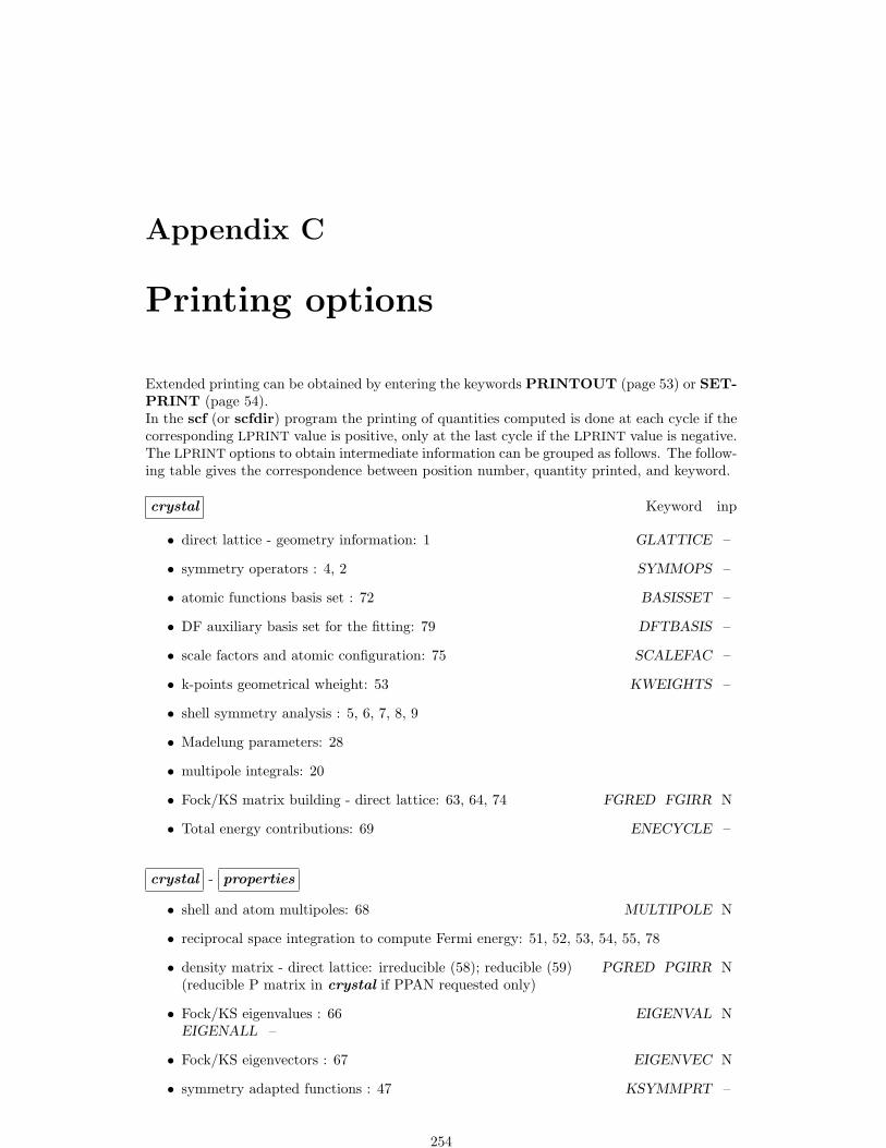
Appendix C

Printing options

Extended printing can be obtained by entering the keywords PRINTOUT (page 53) or SET-PRINT (page 54).In the scf (or scfdir) program the printing of quantities computed is done at each cycle if thecorresponding LPRINT value is positive, only at the last cycle if the LPRINT value is negative.The LPRINT options to obtain intermediate information can be grouped as follows. The follow-ing table gives the correspondence between position number, quantity printed, and keyword.

crystal Keyword inp

• direct lattice - geometry information: 1 GLATTICE –

• symmetry operators : 4, 2 SYMMOPS –

• atomic functions basis set : 72 BASISSET –

• DF auxiliary basis set for the fitting: 79 DFTBASIS –

• scale factors and atomic configuration: 75 SCALEFAC –

• k-points geometrical wheight: 53 KWEIGHTS –

• shell symmetry analysis : 5, 6, 7, 8, 9

• Madelung parameters: 28

• multipole integrals: 20

• Fock/KS matrix building - direct lattice: 63, 64, 74 FGRED FGIRR N

• Total energy contributions: 69 ENECYCLE –

crystal - properties

• shell and atom multipoles: 68 MULTIPOLE N

• reciprocal space integration to compute Fermi energy: 51, 52, 53, 54, 55, 78

• density matrix - direct lattice: irreducible (58); reducible (59) PGRED PGIRR N(reducible P matrix in crystal if PPAN requested only)

• Fock/KS eigenvalues : 66 EIGENVAL NEIGENALL –

• Fock/KS eigenvectors : 67 EIGENVEC N

• symmetry adapted functions : 47 KSYMMPRT –

254

• Population analysis: 70, 73, 77 MULLIKEN N

• Atomic wave-function: 71

properties

• overlap matrix S(g) - direct lattice: 60 (keyword PSIINF) OVERLAP N

• Densities of states: 105, 107 DOSS –

• Projected DOSS for embedding: 36, 37, 38

• DF correlation correction to total energy: 106

• Compton profile and related quantities: 116, 117, 118

• Fermi contact tensor : 18 FTENSOR –

• rotated eigenvectors (keyword ROTREF): 67 EIGENVEC –

• Charge density and electrostatic potential maps: 119 MAPVALUES –

Example

To print the eigenvalues at each scf cycle enter:

PRINTOUTEIGENALLEND

To print the eigenvalues at the first 5 k points at the end of scf only, enter in any input block:

SETPRINT166 -5

Eigenvectors printed by default are from the first valence eigenvector up to the first 6 virtualones. Core and virtual eigenvectors are printed by ”adding” 500 to the selected value ofLPRINT(67). To obtain print all the eigenvectors at the end of scf insert in any input block:

SETPRINT166 -505

255

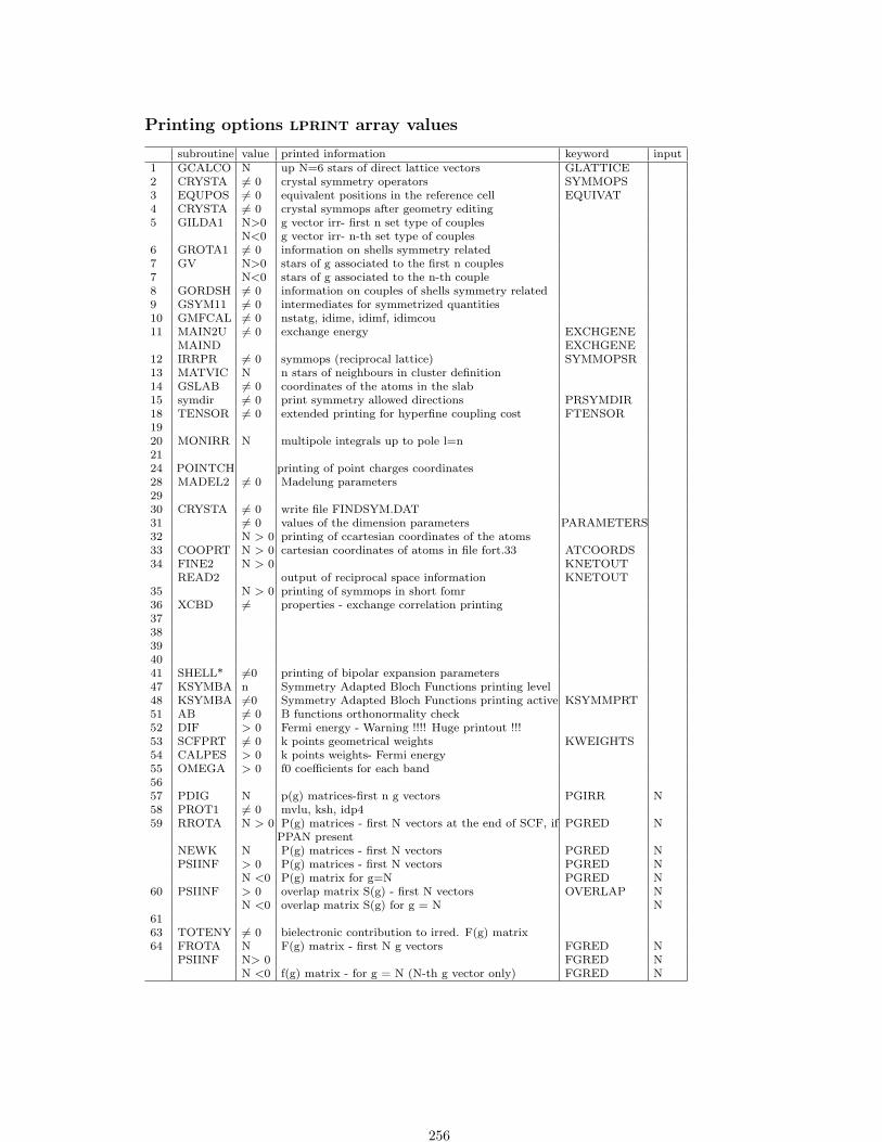
Printing options LPRINT array values

subroutine value printed information keyword input1 GCALCO N up N=6 stars of direct lattice vectors GLATTICE2 CRYSTA 6= 0 crystal symmetry operators SYMMOPS3 EQUPOS 6= 0 equivalent positions in the reference cell EQUIVAT4 CRYSTA 6= 0 crystal symmops after geometry editing5 GILDA1 N>0 g vector irr- first n set type of couples

N<0 g vector irr- n-th set type of couples6 GROTA1 6= 0 information on shells symmetry related7 GV N>0 stars of g associated to the first n couples7 N<0 stars of g associated to the n-th couple8 GORDSH 6= 0 information on couples of shells symmetry related9 GSYM11 6= 0 intermediates for symmetrized quantities10 GMFCAL 6= 0 nstatg, idime, idimf, idimcou11 MAIN2U 6= 0 exchange energy EXCHGENE

MAIND EXCHGENE12 IRRPR 6= 0 symmops (reciprocal lattice) SYMMOPSR13 MATVIC N n stars of neighbours in cluster definition14 GSLAB 6= 0 coordinates of the atoms in the slab15 symdir 6= 0 print symmetry allowed directions PRSYMDIR18 TENSOR 6= 0 extended printing for hyperfine coupling cost FTENSOR1920 MONIRR N multipole integrals up to pole l=n2124 POINTCH printing of point charges coordinates28 MADEL2 6= 0 Madelung parameters2930 CRYSTA 6= 0 write file FINDSYM.DAT31 6= 0 values of the dimension parameters PARAMETERS32 N > 0 printing of ccartesian coordinates of the atoms33 COOPRT N > 0 cartesian coordinates of atoms in file fort.33 ATCOORDS34 FINE2 N > 0 KNETOUT

READ2 output of reciprocal space information KNETOUT35 N > 0 printing of symmops in short fomr36 XCBD 6= properties - exchange correlation printing3738394041 SHELL* 6=0 printing of bipolar expansion parameters47 KSYMBA n Symmetry Adapted Bloch Functions printing level48 KSYMBA 6=0 Symmetry Adapted Bloch Functions printing active KSYMMPRT51 AB 6= 0 B functions orthonormality check52 DIF > 0 Fermi energy - Warning !!!! Huge printout !!!53 SCFPRT 6= 0 k points geometrical weights KWEIGHTS54 CALPES > 0 k points weights- Fermi energy55 OMEGA > 0 f0 coefficients for each band5657 PDIG N p(g) matrices-first n g vectors PGIRR N58 PROT1 6= 0 mvlu, ksh, idp459 RROTA N > 0 P(g) matrices - first N vectors at the end of SCF, if

PPAN presentPGRED N

NEWK N P(g) matrices - first N vectors PGRED NPSIINF > 0 P(g) matrices - first N vectors PGRED N

N <0 P(g) matrix for g=N PGRED N60 PSIINF > 0 overlap matrix S(g) - first N vectors OVERLAP N

N <0 overlap matrix S(g) for g = N N6163 TOTENY 6= 0 bielectronic contribution to irred. F(g) matrix64 FROTA N F(g) matrix - first N g vectors FGRED N

PSIINF N> 0 FGRED NN <0 f(g) matrix - for g = N (N-th g vector only) FGRED N

256

subroutine value printed information keyword input6566 AOFK N e(k)- fock eigenvalues- first N k vectors EIGENVAL N

ADIK NBANDE NDIAG N EIGENALLFDIK NFINE2 NNEWK N

67 AOFK N a(k) - fock eigenvectors - first N k vectors EIGENVEC NADIK NDIAG NFINE2 NNEWK N

68 POLGEN N <0 shell and atom multipoles up to pole l=N MULTIPOL NPOLGEN N >0 atom multipoles up to pole l=N MULTIPOL N

QGAMMA N shell multipoles up to pole l=N MULTIPOL N69 TOTENY 6= 0 contributions to total energy at each cycle ENECYCLE

70FINE2 6= 0 Mulliken population analysis

NEIGHB at the end of scf cyclesPOPAN calls PPBOND, to perform Mulliken analysisPDIBAN

71 PATIRR 6= 0 atomic wave function ATOMICWFPATIR1 6= 0 ” ” ATOMICWF

72 INPBAS 6= 0 basis set BASISSETINPUT2 6= 0 basis set BASISSETREADFG SET

= 173 POPAN 6= 0 Mulliken matrix up to N direct lattice vector MULLIKEN N

PPBONDPDIBAN N

74 TOTENY N f(g) irreducible up to g=N FGIRR NDFTTT2 N FGIRR N

75 INPBAS 6= 0 printing of scale factor and SCALEFACatomic configuration CONFIGAT

7677 PPBOND 0 printing of neighbouring relationship

6= 0 no printing of neighbours relationship78 FERMI 6= 0 informations on Fermi energy calculation

EMIMAN 6= 079

! 79 DFGPRT 6= 0 dft auxiliary basis set - default no printing DFTBASIS! 80 ROTOP > 0 printing of atoms coord. in rotated ref. frame ROTREF

92 INPBAS G94 deck on ft92 GAUSS94

93MOLDRW input deck to MOLDRAW

105 DENSIM < 0 DOSS along energy points DOSS

106DFFIT3 > 0 DFT intermediate printout

(keyword PRINT in dft input)107 STARIN 6= 0 DOSS information112 PROFCA 6= 0 projected DOSS coefficients116 PROFI 6= 0 Compton profile information117 PROFI 6= 0118 PROFI N119 INTEG 6= 0 charge density at grid points MAPVALUES

JJTEG 6= 0 charge density at grid points MAPVALUESMAPNET 6= 0 electrostatic potential at grid points MAPVALUESNAPNET 6= 0 charge density gradient components MAPVALUES

120 LIBPHD 6= 0 extended printing in berny optimizer121 reserved for geometry optimizer122 reserved for geometry optimizer123 reserved for geometry optimizer124 reserved for geometry optimizer125 reserved for geometry optimizer

257

Appendix D

External format

Formatted data are written in files according to the following table:

program keyword ftn filename pg

OPTGEOM 34 optaxxx Geometry input - opt atoms coord. only -See EXTPRT

41

OPTGEOM 34 optcxxx Geometry input - opt cell [atoms] - SeeEXTPRT

41

66 HESSOPT.DAT Hessian matrix68 OPTINFO.DAT Information to restart optimization

crystal GAUSS98 92 GAUSSIAN.DAT Input for GAUSS98 64FINDSYM 26 FINDSYM.DAT data in crystallographic format - read by

program findsym(IUCR)37

STRUCPRT 33 STRUC.INCOOR Cell parameters, coordinates of atoms 56

COORPRT 33 fort.33 Coordinates of the atoms in the cell 37crystal EXTPRT 34 fort.34 Geometry input 41properties PPAN 24 PPAN.DAT Mulliken population analysis 96

properties BAND 25 fort.25 Bands (Crgra2006) 15724 BAND.DAT Bands data 157

CLAS 25 fort.25 Classical potential 159DIEL 24 DIEL.DAT Dielectric constant 160DOSS 25 fort.25 Density of states (IPLOT=1) 162

24 DOSS.DAT Density of states (IPLOT=2) 162ECHG 25 fort.25 Electronic charge density - 2D grid 164

25 RHOLINE.DAT Electronic charge density - 1 grid 164ECH3 31 — Electronic charge density - 3D grid 163

DENS CUBE.DAT Electronic charge density - 3D grid CUBEformat

163

SPIN CUBE.DAT Spin density - 3D grid CUBE format 163POT3 POT CUBE.DAT Electostatic potential - 3D grid CUBE for-

mat183

EMDL 25 fort.25 EMD line (IPLOT=1) 16524 EMDL.DAT EMD line(IPLOT=2) 165

EMDP 25 EMD - 2D grid 261INFOGUI 32 Data for the graphical user interface 168POTC 24 POTC.DAT Electrostatic potential V, Electric field,

Electric field gradient184

POTM 25 fort.25 Electrostatic potential - 2D grid 185PROF 25 fort.25 Compton profile and related quantities

(IPLOT=1)186

24 PROF.DAT Compton profile and related quantities(IPLOT=2)

186

Please refer to the standard script for running CRYSTAL09 as to handle input/output filenames. See:

258

http://www.crystal.unito.it/tutorials =¿ How to run

Data in file fort.25 are read by the programs maps06, doss06, band06 of the packageCrgra2006. In the same run bands, density of states, value of a function in a 2D grid of pointscan be computed. The appropriate command (maps06, doss06, band06) selects and plotsthe selected data .The package can be downloaded from:

http://www.crystal.unito.it/Crgra2006/Crgra2006.html

CLAS - ECHG - POTM - Isovalue maps

The value of the function chosen (classic electrostatic potential (CLAS), charge(+spin) density(ECHG), electrostatic potential (POTM)) is computed in a given net of points. The data arewritten in file fort.25.If the system is spin polarized, total density data are followed by spin density data.

Structure of the file fort.25

1ST RECORD : -%-,IHFERM,TYPE,NROW,NCOL,DX,DY,COSXY format: A3,I1,A4,2I5,3E12.52ND RECORD : XA,YA,ZA,XB,YB,ZB format: 1P,6E12.53RD RECORD : XC,YC,ZC,NAF,LDIM format: 1P,3E12.5,4X,2I44TH RECORDAND FOLLOWING : ((RDAT(I,J),I=1,NROW),J=1,NCOL) format: 1P,6E12.5

Meaning of the variables:

1 ’-%-’ 3 character string marks the beginning of a block of data;1 IHFERM: 0 : closed shell, insulating system

1 : open shell, insulating system2 : closed shell, conducting system - Fermi level can be drawn3 : open shell, conducting system - Fermi level can be drawn

1 TYPE 4 characters string corresponding to the type of data "MAPN"1 NROW number of rows of the data matrix RDAT1 NCOL number of columns of the data matrix RDAT1 DX increment of x (\AA ngstrom) in the plane of the window1 DY increment of y (\AA ngstrom) in the plane of the window1 COSXY cosine of the angle between x and y axis;2 XA,YA,ZA coordinates of the points A,B (see keyword MAPNET) (\AA ngstrom)2 XB,YB,ZB defining the window where the functions is computed (\AA ngstrom)3 XC,YC,ZC coordinates of point C (\AA ngstrom)3 NAF number of atoms in the cell3 LDIM dimensionality (0 molecule; 1 polymer, 2 slab, 3 bulk)4-> ncol*nrow values of the function (a.u.) at the nodes of the grid

naf records follow, with atomic number, symbol, coordinates (Angstrom) of the atoms in the cell:

NAT,SYMBAT,XA,YA,ZA format: I4,1X,A,1P,3E20.12

NAT atomic numberSYMBAT Mendeleev symbolXA,YA,ZA cartesian coordinates of the atoms in the cell (\AA ngstrom)

Cartesian components of cell parameters follow (Angstrom)AX, AY, AZ cartesian component of vector a format: 3E20.12BX, BY, BZ cartesian component of vector b format: 3E20.12CX, CY, CZ cartesian component of vector c format: 3E20.12

The program maps06 looks for the atoms lying in the windows used to compute the function, and itcan draw the symbol of the atoms, the van der Waals sphere, or the bonds between atoms closer thanthe sum of their vdW radii.

ECHG Charge (spin) density - 1D profile

When points B and C coincides in ECHG 8.2 input, coordinates relative to the origin of the segmentand charge density value [coordinate along the line, charge density: charge density derivative x,y,zcomponents] are written with format (2E20.12:3E20.12) in file RHOLINE.DAT. A second set of data,spin density, is written for spin polarized systems, after a blank line.

259

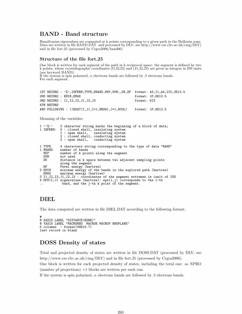
BAND - Band structureHamiltonian eigenvalues are computed at k points corresponding to a given path in the Brillouin zone.Data are written in file BAND.DAT and processed by DLV; see http://www.cse.clrc.ac.uk/cmg/DLV)and in file fort.25 (processed by Crgra2006/band06)

Structure of the file fort.25One block is written for each segment of the path in k reciprocal space: the segment is defined by twok points, whose crystallographic coordinates (I1,I2,I3) and (J1,J2,J3) are given as integers in ISS units(see keyword BAND).If the system is spin polarized, α electrons bands are followed by β electrons bands.For each segment:

1ST RECORD : -%-,IHFERM,TYPE,NBAND,NKP,DUM,,DK,EF format: A3,I1,A4,2I5,3E12.5

2ND RECORD : EMIN,EMAX format: 1P,6E12.5

3RD RECORD : I1,I2,I3,J1,J2,J3 format: 6I3

4TH RECORD

AND FOLLOWING : ((RDAT(I,J),I=1,NROW),J=1,NCOL) format: 1P,6E12.5


1 ’-%-’ 3 character string marks the beginning of a block of data;1 IHFERM: 0 : closed shell, insulating system

1 : open shell, insulating system2 : closed shell, conducting system3 : open shell, conducting system

1 TYPE 4 characters string corresponding to the type of data "BAND"1 NBAND number of bandsNKP number of k points along the segmentDUM not usedDK distance in k space between two adjacent sampling points

along the segmentEF Fermi energy (hartree)

2 EMIN minimum energy of the bands in the explored path (hartree)EMAX maximum energy (hartree)

3 I1,I2,I3,J1,J2,J3 : coordinates of the segment extremes in iunit of ISS4 EPS(I,J) eigenvalues (hartree): eps(i,j) corresponds to the i-th.. band, and the j-th k point of the segment.

DIEL

The data computed are written in file DIEL.DAT according to the following format:

#@ XAXIS LABEL "DISTANCE(BOHR)"@ YAXIS LABEL "MACRORHO MACROE MACROV RHOPLANE"5 columns - format(08E15.7)last record is blank

DOSS Density of states

Total and projected density of states are written in file DOSS.DAT (processed by DLV; seehttp://www.cse.clrc.ac.uk/cmg/DLV) and in file fort.25 (processed by Crgra2006).One block is written for each projected density of states, including the total one: so NPRO(number pf projections) +1 blocks are written per each run.If the system is spin polarized, α electrons bands are followed by β electrons bands.

260

Structure of the file written in file fort.251ST RECORD : -%-,IHFERM,TYPE,NROW,NCOL,DX,DY,COSXY

format : A3,I1,A4,2I5,1P,(3E12.5)2ND RECORD : X0,Y0 format : 1P,6E12.53RD RECORD : I1,I2,I3,I4,I5,I6 format : 6I34TH RECORDAND FOLLOWING : ((RDAT(I,J),I=1,NROW),J=1,NCOL) format : 1P,6E12.5


1 NROW 1 (DOSS are written one projection at a time)NCOL number of energy points in which the DOS is calculatedDX energy increment (hartree)DY not usedCOSXY Fermi energy (hartree)

2 X0 energy corresponding to the first pointY0 not used

3 I1 number of the projection;I2 number of atomic orbitals of the projection;I3,I4,I5,I6 not used

4 RO(J),J=1,NCOL DOS: density of states ro(eps(j)) (atomic units).

Structure of the file written in file DOSS.DAT

Data written in file DOSS.DAT:

1ST RECORD : NPUNTI, NPRO1, IUHFformat : ’# NEPTS’,1X,I5,1X,’NPROJ’,1X,I5,1X,’NSPIN’,1X,I5

2ND RECORD : ’#’3RD RECORD : ’@ YAXIS LABEL "DENSITY OF STATES (STATES/HARTREE/CELL)"’4TH RECORD : (ENE(I),DOSS(IPR,I),IPR=1,NPRO1)AND FOLLOWING :

format : 1P,15E12.4

PROF

The computed quantities are written following the same sequence of the printout. Each recordcontains:

4F coordinate, all electron, core, valence contribution

EMDL

The computed quantities are written following the same sequence of the printout.NPUNTI records are written. Each records contains (FORMAT: 10E12.4)

p (emdl(p,ipro), ipro=1,nprojections))

EMDP

1ST RECORD : -%-,IHFERM,TYPE,NMAX1,NMAX2,PMAX1,PMAX2,COS12

format : A3,I1,A4,2I5,1P,(3E12.5)

2ND RECORD : XDUM,YDUM format : 1P,6E12.5

3RD RECORD : I11,I12,I13,I21,I22,I23 format : 6I3

4TH RECORD

AND FOLLOWING : ((RDAT(I,J),I=1,NMAX1),J=1,NMAX2) format : 1P,6E12.5


1 ’-%-’ 3 character string marks the beginning of a block of data;

1 IHFERM: 0 : closed shell, insulating system

1 : open shell, insulating system

2 : closed shell, conducting system

3 : open shell, conducting system

261

1 TYPE 4 characters string corresponding to the type of data "EMDP"

1 NMAX1 number of points in the first direction

NMAX2 number of points in the second direction

PMAX1 maximum p value along the first direction

PMAX2 maximum p value along the first direction

COSXY angle between the two vectors defining the plane

2 X0 not used

Y0 not used

3 I11,I12,I13 fractional coordinates of the first reciprocal lattice

vector defining the plane

I21,I22,I23 fractional coordinates of the second reciprocal lattice

vector defining the plane

4 RO(J),J=1,NMAX1*NMAX2 electron momentum density at the grid points

(atomic units).

POTC

When ICA 6= 0; NPU 6= 0 (2D or 3D systems) the data computed are written in file POTC.DATaccording to the following format:

#@ XAXIS LABEL "Z (AU)"@ YAXIS LABEL "ELECTROSTATIC PROPERTIES (AU)"@ TITLE "String in the first record in crystal input "@ SUBTITLE "ELECTRIC FIELD INTENSITY: 0.100 AU" ! if external field applied@ LEGEND ON@ LEGEND LENGTH 3@ LEGEND X1 0.87@ LEGEND Y1 0.8@ LEGEND STRING 0 "V"@ LEGEND STRING 1 "E"@ LEGEND STRING 2 "DE/DZ"@ LEGEND STRING 3 "RHO"@ LEGEND STRING 4 "V+VEXT" ! if external field applied@ LEGEND STRING 5 "VEXT" ! if external field appliedNPU records of 5 (7 when external field applied) columns - format 08E15.7

COORPRT

The keyword COORPRT, entered in geometry input or in properties writes in file fort.33(append mode) the following data:

record#

datatype

content

1 I number of atoms (NAF)2 A Title - If written after an SCF calculation, on the same line; totalenergy,

convergence on energy, number of cycles3 A,3F Mendeleev symbol of the atom; x, y, z cartesian coordinates (A)· · · · · ·NAF+2 A,3F Mendeleev symbol of the atom; x, y, z cartesian coordinates (A)

The coordinates of the atoms are written at each geometry optimization cycle (keyword OPT-GEOMThe file ”fort.33” is read by the program MOLDEN [116] which can be downloaded from:www.cmbi.kun.nl/ schaft/molden/molden.html

262

STRUCPRT

The file STRUC.INCOOR is written according to the format given in the example (output forbulk MgO, 2 atoms per cell).

$cell vectors cartesian components of cell parameters (bohr)0.00000000000000 3.97787351190423 3.977873511904233.97787351190423 0.00000000000000 3.977873511904233.97787351190423 3.97787351190423 0.00000000000000

$coordinates cartesian coordinates of atoms (bohr)MG 0.00000000000000 0.00000000000000 0.00000000000000 12O 0.00000000000000 0.00000000000000 -3.97787351190423 8$END

PPAN

# Mulliken Populations:# NSPIN,NATOM n. determinants, number of atoms---- for each atom

# IAT,NSHELL atomic number, number o shells# Xiat,Yiat,Ziat (AU) cartesian coordinates (bohr)# QTOT, QSHELL,I=1,NSHELL atom total electronic charge, (shell charges)# NORB, QORB, I=1,NORB number of orbitals, (orbital electronic charges)

Example:

graphite STO-3G basis set, RHF (1 eterminant)2 atoms, 2 shells per atom, 5 AO per atom

1 2 | 1 determinant, 2 atoms6 2 | 1st atom: atomic number 6, 2 shells

-1.320 -2.287 0.000 | cartesian coordinates 1st atom6.000 1.993 4.007 | 6, electronic charge of 1st atom

| 1.993 electronic charge of 1st shell (1s)| 4.007 electronic charge of 2nd shell (2sp)

5 | 5 atomic orbitals1.993 1.096 0.956 0.956 1.000| 1.993 electronic charge of 1st AO (1s)

| 1.096 electronic charge of 2nd AO (2s)| 0.956 electronic charge of 3rd AO (px)| 0.956 electronic charge of 4th AO (py)| 1.000 electronic charge of 5th AO (pz)

6 2 | 2nd atom: atomic number 6, 2 shells-2.640 0.000 0.000 | cartesian coordinates 2nd atom6.000 1.993 4.007 | 6, electronic charge of 1st atom

| 1.993 electronic charge of 1st shell (1s)| 4.007 electronic charge of 2nd shell (2sp)

5 | 5 atomic orbitals1.993 1.096 0.956 0.956 1.000| 1.993 electronic charge of 1st AO (1s)

| 1.096 electronic charge of 2nd AO (2s)| 0.956 electronic charge of 3rd AO (px)| 0.956 electronic charge of 4th AO (py)| 1.000 electronic charge of 5th AO (pz)

6 2 | second atom: atomic number 6, 2 shells-2.640 0.000 0.000 | cartesian coordinates 2nd atom

263

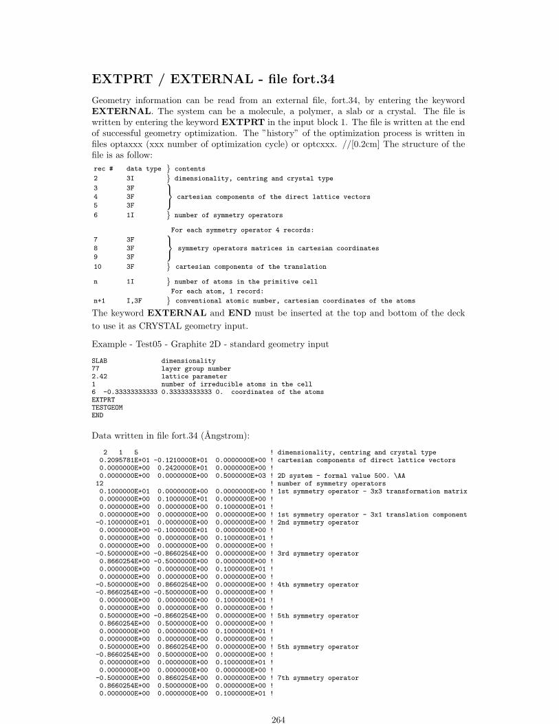
EXTPRT / EXTERNAL - file fort.34

Geometry information can be read from an external file, fort.34, by entering the keywordEXTERNAL. The system can be a molecule, a polymer, a slab or a crystal. The file iswritten by entering the keyword EXTPRT in the input block 1. The file is written at the endof successful geometry optimization. The ”history” of the optimization process is written infiles optaxxx (xxx number of optimization cycle) or optcxxx. //[0.2cm] The structure of thefile is as follow:rec # data type

¯contents

2 3I¯

dimensionality, centring and crystal type

3 3F

4 3F

5 3F

9=; cartesian components of the direct lattice vectors

6 1I¯

number of symmetry operators

For each symmetry operator 4 records:

7 3F

8 3F

9 3F

9=; symmetry operators matrices in cartesian coordinates

10 3F¯

cartesian components of the translation

n 1I¯

number of atoms in the primitive cell

For each atom, 1 record:

n+1 I,3F¯

conventional atomic number, cartesian coordinates of the atoms

The keyword EXTERNAL and END must be inserted at the top and bottom of the deckto use it as CRYSTAL geometry input.

Example - Test05 - Graphite 2D - standard geometry input

SLAB dimensionality77 layer group number2.42 lattice parameter1 number of irreducible atoms in the cell6 -0.33333333333 0.33333333333 0. coordinates of the atomsEXTPRTTESTGEOMEND

Data written in file fort.34 (Angstrom):

2 1 5 ! dimensionality, centring and crystal type0.2095781E+01 -0.1210000E+01 0.0000000E+00 ! cartesian components of direct lattice vectors0.0000000E+00 0.2420000E+01 0.0000000E+00 !0.0000000E+00 0.0000000E+00 0.5000000E+03 ! 2D system - formal value 500. \AA

12 ! number of symmetry operators0.1000000E+01 0.0000000E+00 0.0000000E+00 ! 1st symmetry operator - 3x3 transformation matrix0.0000000E+00 0.1000000E+01 0.0000000E+00 !0.0000000E+00 0.0000000E+00 0.1000000E+01 !0.0000000E+00 0.0000000E+00 0.0000000E+00 ! 1st symmetry operator - 3x1 translation component

-0.1000000E+01 0.0000000E+00 0.0000000E+00 ! 2nd symmetry operator0.0000000E+00 -0.1000000E+01 0.0000000E+00 !0.0000000E+00 0.0000000E+00 0.1000000E+01 !0.0000000E+00 0.0000000E+00 0.0000000E+00 !

-0.5000000E+00 -0.8660254E+00 0.0000000E+00 ! 3rd symmetry operator0.8660254E+00 -0.5000000E+00 0.0000000E+00 !0.0000000E+00 0.0000000E+00 0.1000000E+01 !0.0000000E+00 0.0000000E+00 0.0000000E+00 !

-0.5000000E+00 0.8660254E+00 0.0000000E+00 ! 4th symmetry operator-0.8660254E+00 -0.5000000E+00 0.0000000E+00 !0.0000000E+00 0.0000000E+00 0.1000000E+01 !0.0000000E+00 0.0000000E+00 0.0000000E+00 !0.5000000E+00 -0.8660254E+00 0.0000000E+00 ! 5th symmetry operator0.8660254E+00 0.5000000E+00 0.0000000E+00 !0.0000000E+00 0.0000000E+00 0.1000000E+01 !0.0000000E+00 0.0000000E+00 0.0000000E+00 !0.5000000E+00 0.8660254E+00 0.0000000E+00 ! 5th symmetry operator

-0.8660254E+00 0.5000000E+00 0.0000000E+00 !0.0000000E+00 0.0000000E+00 0.1000000E+01 !0.0000000E+00 0.0000000E+00 0.0000000E+00 !

-0.5000000E+00 0.8660254E+00 0.0000000E+00 ! 7th symmetry operator0.8660254E+00 0.5000000E+00 0.0000000E+00 !0.0000000E+00 0.0000000E+00 0.1000000E+01 !

264

0.0000000E+00 0.0000000E+00 0.0000000E+00 !0.1000000E+01 0.0000000E+00 0.0000000E+00 ! 8th symmetry operator0.0000000E+00 -0.1000000E+01 0.0000000E+00 !0.0000000E+00 0.0000000E+00 0.1000000E+01 !0.0000000E+00 0.0000000E+00 0.0000000E+00 !

-0.5000000E+00 -0.8660254E+00 0.0000000E+00 ! 9th symmetry operator-0.8660254E+00 0.5000000E+00 0.0000000E+00 !0.0000000E+00 0.0000000E+00 0.1000000E+01 !0.0000000E+00 0.0000000E+00 0.0000000E+00 !0.5000000E+00 0.8660254E+00 0.0000000E+00 ! 10th symmetry operator0.8660254E+00 -0.5000000E+00 0.0000000E+00 !0.0000000E+00 0.0000000E+00 0.1000000E+01 !0.0000000E+00 0.0000000E+00 0.0000000E+00 !

-0.1000000E+01 0.0000000E+00 0.0000000E+00 ! 11th symmetry operator0.0000000E+00 0.1000000E+01 0.0000000E+00 !0.0000000E+00 0.0000000E+00 0.1000000E+01 !0.0000000E+00 0.0000000E+00 0.0000000E+00 !0.5000000E+00 -0.8660254E+00 0.0000000E+00 ! 12th symmetry operator

-0.8660254E+00 -0.5000000E+00 0.0000000E+00 !0.0000000E+00 0.0000000E+00 0.1000000E+01 !0.0000000E+00 0.0000000E+00 0.0000000E+00 !1 ! number of irreducible atoms in the primitive cell

6 -0.6985938 -1.2100000 0.0000000 ! conventional atomic number, cartesian coordinate

ECH3/POT3/GRID3D

Functions values computed at 3D grid of points by the keywords ECH3 (page 163), POT3(page183), GRID3D (page167) are written according to two formats: . All data in atomicunits.

1. Fortran unit 31 is written According to the following format. All data in atomic units.

rec # data type¯

contents

1 A¯

title: charge density /spin density

2 3I¯

npa,npb,npc, number of points along the 3 directions

3 3E¯

x,y,z cartesian coordinates of the point (1,1,1)

4 3E¯

dxa, dya, dza cartesian components of the step along a

5 3E¯

dxb, dyb, dzb cartesian components of the step along b

6 3E¯

dxc, dyc, dzc cartesian components of the step along c

7 ... 5E¯

npa*npb*npc floating point data, 5/record

2. Function data computed at 3D grid points are written according to GAUSSIAN CUBEformat in files:

DENS CUBEDAT charge densitySPIN CUBEDAT spin densityPOT CUBEDAT electrostatic potential

INFOGUI

Fortran unit 32 is written through the keyword INFOGUI (page 168). The format is almostself-explaining. The following data are written for MgO bulk (test11).

2 atom(s) per cell6 shells

18 atomic orbitals20 electrons per cell12 core electrons per cellNo eigenvalue level shiftingNo Alpha-Beta Spin lockingNo N. Beta Spin lockingType of Calculation: RESTRICTED CLOSED SHELLTotal Energy = -0.27466415E+03H

265

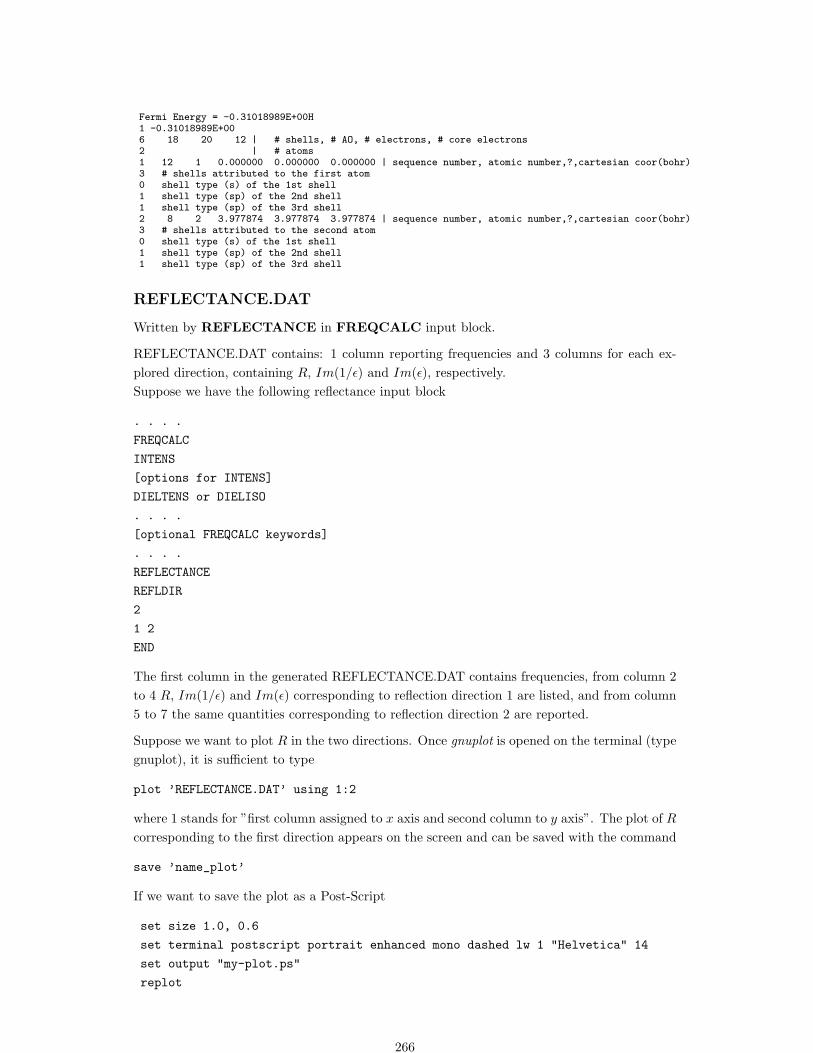
Fermi Energy = -0.31018989E+00H1 -0.31018989E+006 18 20 12 | # shells, # AO, # electrons, # core electrons2 | # atoms1 12 1 0.000000 0.000000 0.000000 | sequence number, atomic number,?,cartesian coor(bohr)3 # shells attributed to the first atom0 shell type (s) of the 1st shell1 shell type (sp) of the 2nd shell1 shell type (sp) of the 3rd shell2 8 2 3.977874 3.977874 3.977874 | sequence number, atomic number,?,cartesian coor(bohr)3 # shells attributed to the second atom0 shell type (s) of the 1st shell1 shell type (sp) of the 2nd shell1 shell type (sp) of the 3rd shell

REFLECTANCE.DAT

Written by REFLECTANCE in FREQCALC input block.

REFLECTANCE.DAT contains: 1 column reporting frequencies and 3 columns for each ex-plored direction, containing R, Im(1/ε) and Im(ε), respectively.Suppose we have the following reflectance input block

. . . .

FREQCALC

INTENS

[options for INTENS]

DIELTENS or DIELISO

. . . .

[optional FREQCALC keywords]

. . . .

REFLECTANCE

REFLDIR

2

1 2

END

The first column in the generated REFLECTANCE.DAT contains frequencies, from column 2to 4 R, Im(1/ε) and Im(ε) corresponding to reflection direction 1 are listed, and from column5 to 7 the same quantities corresponding to reflection direction 2 are reported.

Suppose we want to plot R in the two directions. Once gnuplot is opened on the terminal (typegnuplot), it is sufficient to type

plot ’REFLECTANCE.DAT’ using 1:2

where 1 stands for ”first column assigned to x axis and second column to y axis”. The plot of Rcorresponding to the first direction appears on the screen and can be saved with the command

save ’name_plot’

If we want to save the plot as a Post-Script

set size 1.0, 0.6

set terminal postscript portrait enhanced mono dashed lw 1 "Helvetica" 14

set output "my-plot.ps"

replot

266

Further details about these commands and manipulation of files at http://www.duke.edu/ hp-gavin/gnuplot.html and http://www.gnuplot.info/documentation.html.

In a similar way, we can type

plot ’REFLECTANCE.DAT’ using 1:5

in order to obtain R along the second reflection direction.

Interface to external programs

The keyword CRYAPI OUT, present into properties input stream writes formatted wavefunction information, both in direct and reciprocal space, in file GRED.DAT and KRED.DATThe scripts runcry06 and runprop06 save them in the current directory as inpfilename.GREDand inpfilename.KRED .The program cryapi inp, written in fortran 90, is distributed as source code(http://www.crystal.unito.it => documentation => utilities). It reads and prints the data,showing the meaning of the variables and the organization of datacryapi inp should be compiled by any fortran 90 compiler: comments and request for moreinformation are welcome (mail to [email protected]).

GRED.DAT

The file GRED.DAT contains:

• Geometry, symmetry operators;

• Local functions basis set (including ECP)

• Overlap matrix in direct lattice

• Hamiltonian matrix in direct lattice

• Density matrix in direct lattice

• Wannier functions (if file fort.80, written by LOCALWF when localization is successful,is present)

Overlap, hamiltonian, density matrices are written as arrays of non-zero elements. GRED.DATcontains the information to build full matrices.All data are printed executing cryapi inp

KRED.DAT

The file KRED.DAT is written if eigenvectors have been computed (keyword NEWK 8.2) byproperties.CRYSTAL works in the irreducible Brillouin (IBZ) zone only: eigenvectors in the full Brillouinzone (BZ) are computed by rotation, and by time reversal symmetry, when necessary. The fileKRED.DAT contains:

• Coordinates of k points in irreducible Brillouin zone, according to Pack-Monkhorst net

• Symmetry operators in reciprocal lattice

267

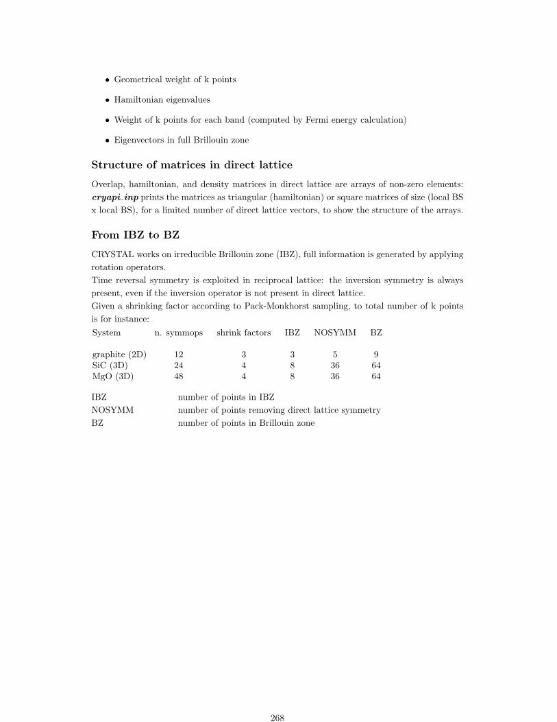
• Geometrical weight of k points

• Hamiltonian eigenvalues

• Weight of k points for each band (computed by Fermi energy calculation)

• Eigenvectors in full Brillouin zone

Structure of matrices in direct lattice

Overlap, hamiltonian, and density matrices in direct lattice are arrays of non-zero elements:cryapi inp prints the matrices as triangular (hamiltonian) or square matrices of size (local BSx local BS), for a limited number of direct lattice vectors, to show the structure of the arrays.

From IBZ to BZ

CRYSTAL works on irreducible Brillouin zone (IBZ), full information is generated by applyingrotation operators.Time reversal symmetry is exploited in reciprocal lattice: the inversion symmetry is alwayspresent, even if the inversion operator is not present in direct lattice.Given a shrinking factor according to Pack-Monkhorst sampling, to total number of k pointsis for instance:System n. symmops shrink factors IBZ NOSYMM BZ

graphite (2D) 12 3 3 5 9SiC (3D) 24 4 8 36 64MgO (3D) 48 4 8 36 64

IBZ number of points in IBZNOSYMM number of points removing direct lattice symmetryBZ number of points in Brillouin zone

268

Appendix E

Normalization coefficients

A. Bert - Thesis 2002

The aim of this appendix is to show how normalization coefficients of the basis functions aredefined in CRYSTAL and to describe how they are stored in the program.

Basic Definitions

Let us consider a function, f(r); we have in general:∫dr |f(r)|2 6= 1; (E.1)

however, we can always define a related f ′(r), multiplying f(r) by a constant N :

f ′(r) = Nf(r), (E.2)

such that: ∫dr |f ′(r)|2 = 1. (E.3)

f ′(r) is said to be a normalized function and N is its Normalization Coefficient (NC). Substi-tuting eq. E.2 in E.3, we have:

N =(∫

dr |f(r)|2)−1/2

. (E.4)

Gaussians: Product Theorem and Normalization

Let us define Gaussian functions as:

G(αi; r−A) = exp(−αi(r−A)2), (E.5)

where A is the centroid of the function.The Gaussian product theorem states that the product of two Gaussians, is still a Gaussianfunction:1

G(α; r−A)G(β; r−B) = exp(−αβξ|R|2

)G(ξ; r−P); (E.8)

1Let us prove the Gaussian product theorem:

G(α; r − A)G(β; r − B) = exp(−αi(r − A)2) exp(−αj(r − B)2

= exp`−α(r2 + A2 + 2rA) − β(r2 + B2 + 2rB)

´= exp

»−ξ

„(r − P)2 + P2 −

αA2 + βB2

ξ

«–. (E.6)

269

with:

ξ = α+ β, (E.9)

P =αA + βB

ξ, (E.10)

R = A−B. (E.11)

From eq. E.4, the NC of Gaussian functions, gi, can be written as:

gi =(∫

dr (G(αi; r))2

)−1/2

=(∫

drG(2αi; r))−1/2

=(π

2αi

)−3/4

, (E.12)

where the Gaussian product theorem and the Gaussian integral [130] have been used. G′(αi; r),defined as:

G′(αi; r) = giG(αi; r), (E.13)

is a normalized function.

Harmonic Gaussians

The Definition

The Solid Harmonic Functions, Y m` , [110] are defined as:

Y m` (r) = r`P

|m|` (cosϑ)eimφ, (E.14)

where Pm` is the Legendre Polynomial Function characterized by the integers ` and m, such

that: ` ≥ 0 and −` ≤ m ≤ `. [1]Starting from Y m

` , the Real Solid Harmonic, Xm` , can be defined:

X|m|` (r) = <(Y |m|

` ) =Y|m|` (r) + Y

−|m|` (r)

2, (E.15)

X−|m|` (r) = =(Y |m|

` ) =Y|m|` (r)− Y

−|m|` (r)

2i. (E.16)

We report some examples of X functions.` = 0:

X00 (r) = 1; (E.17)

` = 1:X0

1 (r) = z, X11 (r) = x, X−1

1 (r) = y; (E.18)

` = 2:X0

2 (r) = z2 − 0.5(x2 − y2), X12 (r) = 3zx, X−1

2 (r) = 3zy, (E.19)

X22 (r) = 3(x2 + y2), X−2

2 (r) = 3xy. (E.20)

Using eqs. E.9, E.10 and E.11, eq. E.6 can be rewritten as:

G(α; r − A)G(β; r − B) = exp

„−

αβ

ξ|R|2

«G(ξ; r − P). (E.7)

270

We have now the tools required to define the Solid Harmonic Gaussian, [110] ξ:

ξn`m(αi; r) = |r|2nY m` (r)Gi(αi; r), (E.21)

where n is a non-negative integer number (n ≥ 0). We are interested here only in n = 0harmonic Gaussians (that is, ξ0`m), so we shall simply write (omitting the n = 0 index):

ξ`m(αi; r) = Y m` (r)G(αi; r). (E.22)

Substituting Y with X (eqs. E.15 and E.16) in eq. E.22, Real Harmonic Gaussians, γ, can bedefined:

γ`m(αi; r) = Xm` (r)G(αi; r). (E.23)

γ are used as basis functions in the CRYSTAL program and are related to the ξ ones byfollowings relations:

γ`|m| =ξ`|m| + ξ`−|m|

2, (E.24)

γ`−|m| =ξ`|m| − ξ`−|m|

2i, (E.25)

where eqs. E.15 and E.16 have been used.Note that, when ` is equal to 0, ξ and γ functions degenerate to simple Gaussians:

ξ00 = γ00 = G, (E.26)

where eq. E.17 has been used and ξ degenerates to γ when m = 0:

ξ`0 = γ`0, (E.27)

where eqs. E.24 and E.25 have been used.

The Normalization Coefficient

Let us consider now ξ and γ’s normalization coefficients (b and c, respectively), from eq. E.4,follows:

b`mi = (Ξ)−1/2 (E.28)

c`mi = (Υ)−1/2, (E.29)

where

Ξ =∫dr∣∣ξ`m(αi; r)

∣∣2 (E.30)

Υ =∫dr(γ`m(αi; r)

)2. (E.31)

Using eqs. E.5, E.8, E.14, E.22 and a spherical polar coordinate system,2 the Ξ integral can befactorized as:

Ξ =∫dr [Y m

` (r)G(αi; r)]∗Y m

` (r)G(αi; r)

=∫drY −m

` (r)Y m` (r)G(2αi; r)

= Ξr Ξϑ Ξφ, (E.32)

2dr = r2sinϑ dr dϑ dφ

271

with:

Ξr =∫ ∞

0

dr exp(−2αir2)r2`+2

=Γ(`+ 3/2)2(2αi)`+3/2

=π1/2(2`+ 1)!!2`+2(2αi)`+3/2

, (E.33)

where we have used the Γ function’s properties; [1]

Ξϑ =∫ π

0

dϑ(P|m|` (cosϑ)

)2

sinϑ

=2(`+ |m|)!

(2`+ 1)(`− |m|)!, (E.34)

where the Legendre polynomials’ properties have been used, [1] and

Ξφ =∫ 2π

0

dφ = 2π. (E.35)

Substituting eqs. E.32, E.33, E.34 and E.35 in the b definition (eq. E.28) we obtain:

b`mi =π1/2(2`+ 1)!!2`+2(2αi)`+3/2

2(`+ |m|)!(2`+ 1)(`− |m|)!

2π

=

(π3/2 (2`− 1)!! (`+ |m|)!22`+3/2 α

`+3/2i (`− |m|)!

)−1/2

. (E.36)

Note that b is independent from the sign of m (as Ξ is), that is:

b`|m|i = b

`−|m|i . (E.37)

In order to deduce the explicit expression for c, we are interested now in solving the integralof eq. E.31:

Υ =∫dr (Xm

` (r))2 G(2αi; r), (E.38)

where eqs. E.8 and E.23 have been used. Substituting eq. E.24 (γ functions with m ≥ 0) inprevious equation, we have:

Υm≥0 =14

(∫dr∣∣∣ξ`|m|(αi; r)

∣∣∣2 +∫dr∣∣∣ξ`−|m|(αi; r)

∣∣∣2 +

+ 2∫dr ξ`|m|(αi; r)ξ`−|m|(αi; r)

). (E.39)

The first two integrals in eq. E.39 can be recognized as Ξ (eq. E.32, reminding that Ξ isindependent from the m sign); the last one, if m 6= 0, is null for the orthogonality propertiesof the Harmonic functions, [1] therefore:

Υm>0 =Ξ2. (E.40)

The same result is found for negative m, substituting eq. E.25 (instead of eq. E.24, as done)in eq. E.31:

Υm<0 =Ξ2, (E.41)

272

so Υ (as Ξ is) is independent from the m sign. If m = 0, the last integral in eq. E.39 is equalto Ξ, as the first two ones:

Υm=0 = Ξ; (E.42)

the previous equation can be deduced also from eq. E.27.Summarizing, from eqs. E.40, E.41 and E.42, we get:

Υ =Ξ

2− δm0(E.43)

and, finally, substituting eqs. E.32 and E.43 in eq. E.29, we obtain:

c`mi =

(π3/2 (2`− 1)!! (`+ |m|)!

22`+3/2(2− δm0)α`+3/2i (`− |m|)!

)−1/2

. (E.44)

The c expression (eq. E.44) can be reorganized in a two factors formula:

c`mi = a`i f

`m, (E.45)

with:

a`i =

(π3/2

(2αi)`+3/2

)−1/2

, (E.46)

the α-dependent term, and

f `m =(

(2`− 1)!! (`+ |m|)!2`(2− δm,0)(`− |m|)!

)−1/2

, (E.47)

the m dependent term.Note that,

• If ` = 0, γ degenerates in a simple Gaussian (eq. E.26),

f00 = 1 and c00i = a0i = gi, (E.48)

where gi is the G’s NC (eq. E.12).

• If ` = 1, f1m = 1/2 for the three m-values:

f1m = 1/2 and c1mi =

a1i

2=α

5/4i 27/4

π3/4, ∀ m = −1, 0, 1. (E.49)

• If ` = 2, we have:

c20i =α

7/4i 211/4

π3/4√

3; c21i = c2−1

i =α

7/4i 211/4

π3/43; c22i = c2−2

i =α

7/4i 27/4

π3/43. (E.50)

Let us verify, for two examples, thatγ′ = c γ (E.51)

is a normalized function, proving that the following integral, I, is equal to 1,

I`mi =

∫dr(c`mi γ`m(αi; r)

)2. (E.52)

273

The s Case (` = 0, m = 0)

I00i =

(c00i

)2 ∫dr(γ00(αi; r)

)2= (gi)2

∫dr (G(αi; r))

2

=(∫

(G(αi; r))2dr)−1 ∫

(G(αi; r))2dr = 1, (E.53)

where eqs. E.48, E.27 and E.12 have been used.

A d Case (` = 2, m = 1)

I21i =

∫dr(c21i γ

21(αi; r))2

=(c21i

)2J, (E.54)

with:J =

∫dr (3zxG(2αi; r))

2, (E.55)

where eqs. E.23 and E.19 have been used.Gaussians are separable functions, that is:

G(αi; r) = Gx(αi;x)Gy(αi; y)Gz(αi; z), (E.56)

with:Gx(αi;x) = exp(−αix

2) (E.57)

and similarly for y and z. Substituting eq. E.56 in eq. E.55, we have:

J = 9JxJyJz, (E.58)

with:

Jx =∫x2Gx(2αi;x)dx =

√π

2(2αi)−3/2, (E.59)

Jy =∫Gy(2αi; y)dy =

(π

2αi

)1/2

, (E.60)

Jz =∫z2Gz(2αi; z)dz =

√π

2(2αi)−3/2, (E.61)

where ref. [130] has been used in solving the integrals. Substituting now eqs. E.49 and E.58 ineq. E.54, we obtain:

I21i =

α7/2i 211/2

π3/2 99(√

π

2(2αi)−3/2

)2(π

2αi

)1/2

= 1. (E.62)

Atomic Orbitals Normalization

The variational basis functions of the CRYSTAL program (AOs), ϕµ, are normalized contrac-tions (fixed linear combinations) of normalized real solid harmonic Gaussian type functions(primitive functions), γ′ (eq. E.51). The AOs are organized in shells, ϕµ belonging to thesame shell, λ, have same radial part, that is, same contraction coefficients, dλ

i , same Gaussianexponents, αλ

i and different angular part, Xm` :

ϕ`mλ = Nλ

∑i

dλi c

`mi γ`m(αλ

i ; r) = Nλ

∑i

dλi c

`mi Xm

` (r)G(αλi ; r). (E.63)

274

The index i runs over the primitive functions of the contraction, dλi is the contraction coefficient

of the i-th primitive in shell λ and, as we have seen, it is the same for all the AOs of λ, thatis, it does not depend on ` or m. γ and c are the primitive function and its NC (eq. E.29),respectively. Nλ is the NC of AOs belonging to λ and is defined as:

Nλ =

∫ dr

(∑i

dλi c

`mi γ`m(αλ

i ; r)

)2−1/2

, (E.64)

in the following will be shown that N depends only on the shell, λ.We report, as an example, the three AOs of a p-type shell (` = 1), supposing that λ is classifiedas the fourth shell of the unitary cell and each AO is a contraction of two primitives.

pz = ϕ104 = N4

(d41 c

101 γ10(α4

1; r) + d42 c

102 γ10(α4

2; r)), (E.65)

px = ϕ114 = N4

(d41 c

111 γ11(α4

1; r) + d42 c

112 γ11(α4

2; r)), (E.66)

py = ϕ1−14 = N4

(d41 c

1−11 γ1−1(α4

1; r) + d42 c

1−12 γ1−1(α4

2; r)). (E.67)

Let us put our attention on Nλ. Eq. E.64 can be rewritten as:

Nλ =

∑i,j

dλi d

λj c

`mi c`mj Υ′

−1/2

, (E.68)

with:Υ′ =

∫dr γ`m(αi; r) γ`m(αj ; r), (E.69)

where the shell index on α has been omitted for simplicity. Substituting eq. E.23 in eq. E.69,we have:

Υ′ =∫Xm

` (r)G(αi; r)Xm` (r)G(αj ; r)dr =

∫(Xm

` (r))2G[(αi + αj); r]dr, (E.70)

where the Gaussian product theorem (eq. E.8) has been used.From eq. E.31, it can be seen that Υ′ differs from Υ only in the Gaussian exponent (αi + αj

instead of 2αi), using then eqs. E.43, E.32, E.34 and E.35, Υ′ is rewritten as:

Υ′ =Υ′

r Ξϑ Ξϕ

2− δm0, (E.71)

with:

Υ′r =

∫ ∞

0

dr exp[−(αi + αj)r2]r2`+2

=Γ(`+ 3/2)

2(αi + αj)`+3/2

=π1/2(2`+ 1)!!

2`+2(αi + αj)`+3/2. (E.72)

Substituting eqs. E.44, E.71 and E.72 in eq. E.68, we obtain:

Nλ =

∑i,j

dλi d

λj

2√αλ

i αλj

αλi + αλ

j

`+3/2−1/2

, (E.73)

where it is clear that N depends only on λ.

275

The Code

In order to explain easily the organization of NCs in CRYSTAL, eq. E.63 is reorganized asfollows:

ϕ`mλ =

∑i

n`mλ,i γ

`m(αλi ; r), (E.74)

with:n`m

λ,i = Nλ dλi c

`mi . (E.75)

Note that, while the AO is normalized, the function γ′′ = nγ is not; in fact n is not anormalization factor, and it will be referred as the pre-Gaussian factor.At the moment the CRYSTAL code is able to treat four type of shells: s, sp, p and d.3 Ans shell has only an AO, that is a contraction of simple Gaussians (` = 0); in a p one thereare three AOs (different for the m value, px, py and pz) with ` = 1 primitives; d shells areobviously formed by five ` = 2 AOs. The three basis functions of a sp shell are contractions ofone s primitive function and several ps’.In the calculation of the integrals required in the SCF process, n must be very often multipliedby the constant factor π5/8 21/4; [103] therefore, in the code, pre-Gaussian factors are notstored, but the following quantities, that we shall call code pre-Gaussian constants:

Sλi = π5/8 21/4 n00

λ,i (E.76)

Pλi = π5/8 21/4 n1m

λ,i ∀ m = 0, 1,−1 (E.77)

Dλi = π5/8 21/4

√(2 + |m|)!

(2− δm0)(2− |m|)!n2m

λ,i ∀ m = 0, 1,−1, 2,−2. (E.78)

Note that the square root in eq. E.78 (the inverse of the m-dependent part of c, eq. E.44)makes D independent from the m value, whereas n2m

λ,i depends from it. In such a way, S, P

and D are m-independentIn the inpbas routine, contraction coefficients (as defined in input), dλ

i , related to s, p and d

AOs, are loaded in the two dimension packed arrays c1, c2 and c3, respectively (they are storedin the module basato module). Their length corresponds to the total number of primitivesin the unit cell and is the same for the three arrays. The first elements are the contractioncoefficients for the first shell (d1

i ), then the d2i s (second shell) follows, and so on; the contraction

index, i, is the internal one. For an s shell, for example, the elements of c2 and c3 are null, ofcourse.In the gaunov routine, c1, c2 and c3 are redefined and loaded with the code pre-Gaussianconstants S, P and D, respectively; naturally they maintain the described organization andmodule basato module is overwritten.In gaunov two further arrays, c2w and c3w (that follow the convention used in the ATMOLprogram) are also defined and loaded in basato module. They have the same organization asc1, c2 and c3 and contain P′λi and D′λ

i coefficients, respectively:

P′λi =π5/8 21/4

2αin1m

λ,i ∀ m = 0, 1,−1 (E.79)

D′λi =

π5/8 21/4

(2αi)2

√(2 + |m|)!

(2− δm0)(2− |m|)!n2m

λ,i ∀ m = 0, 1,−1, 2,−2. (E.80)

3The implementation of higher polynomial functions is now in progress.

276

We give an example of evaluation of an overlap integral Sµν over an s and a m = 0 d AO(ϕµ ≡ ϕλ

00, ϕν ≡ ϕσ20) sitting in the reference cell:

Sµν =∫drϕλ

00(r)ϕσ20(r). (E.81)

Substituting eq. E.74 in the previous equation, we have:

Sµν =∑ij

n00λ,i n

20σ,j

∫dr γ00(αλ

i ; r)γ20(ασj ; r). (E.82)

Since in the code, S and D are available (but not the n coefficients), we express n as a functionof code pre-Gaussian constants, using eqs. E.76 and E.78, and we rewrite the overlap integralas:

Sµν =(π5/8 21/4

)−2

√(2− δm0)(2− |m|)!

(2 + |m|)!∑ij

Sλi Dσ

i

∫dr γ00(αλ

i ; r)γ20(ασj ; r). (E.83)

Note that the m-dependent term contained in n, for d shells, must be multiplied a posteriori,because is not included in D. This operation is performed in the dfac3 routine, that providesMcMurchie-Davidson coefficients multiplied by code pre-Gaussian constants and, when λ is ad shell, by the m-dependent part of n2m

λ,i .

277

Appendix F

CRYSTAL09 versus CRYSTAL06

Geometry

• Roto-translational symmetryIn the case of polymers it can treat helical structures (translation followed by a rota-tion around the periodic axis). See keyword HELIX (page 15) and examples therein.CRYSTAL06 allowed commensurate rotations only, by adopting a suitably large unit cell.

• NanotubesA special input option allows generation of 1D structures (nanotubes) from 2D one. Seekeyword NANOTUBE (page 47).

Geometry optimization

• Default choice modified: TRUSTRADIUS scheme active.

Use keyword NOTRUSTR in OPTGEOM input block (page 111) to run geometryoptimization with CRYSTAL06 default.

Frequencies calculation

• default value for SCF convergence on total energy is 10−9

• default choice for numerical integration grid (DFT Hamiltonian): XLGRID. To runDFT Hamiltonian cases with CRYSTAL06 numerical integration accuracy insert LGRIDin DFT input block (page 78)

• default choice to compute IR intensities: Berry phase approach. To compute IR intensi-ties with CRYSTAL09 as with CRYSTAL06 insert keyword INTLOC in FREQCALCinput block.

Basis set

• f orbitals- f orbitals (local functions basis set) with non-zero occupancy allowed. This new featureallows study of systems with Lanthanides.d and f orbitals occupation guess- FDOCCUP (input block3, page 84) defines the occupation of specific f or d orbitals

278

in a given shell in the SCF initial guess, according to the local atomic symmetry in thecrystal lattice.

• - Effective core pseudo potentials Projector operators up to angular quantum number` = 4 are allowed. Input deck has been changed

279

Test casescrystal09 versus crystal06 total energies (hartree)

CRYSTAL06 CRYSTAL09 diff

TEST 0 -110.7649354541 -110.7649354541 0.00E+00

TEST 1 -39.7267242374 -39.7267242374 0.00E+00

TEST 2 -223.7874756819 -223.7874756819 0.00E+00

TEST 3 -893.8746580004 -893.8746580004 0.00E+00

TEST 4 -1400.1776585535 -1400.1776585535 0.00E+00

TEST 5 -74.8333583570 -74.8333583570 1.01E-12

TEST 6 -58.4208255980 -58.4208255980 1.00E-12

TEST 7 -2800.7355953744 -2800.7355953744 0.00E+00

TEST 8 -571.3207540595 -571.3207540595 3.00E-11

TEST 9 -29.2566111179 -29.2566111179 0.00E+00

TEST10 -577.8265583253 -577.8265583271 -1.86E-09

TEST11 -274.6641530559 -274.6641530559 -3.00E-11

TEST12 -447.6810664796 -447.6810664796 -6.00E-11

TEST13 -23.9856901143 -23.9856901143 0.00E+00

TEST14 -159.6970601598 -159.6970601598 0.00E+00

TEST15 -5229.8366027793 -5229.8366027783 1.00E-09

TEST16 -2995.2869386583 -2995.2869386582 1.00E-10

TEST17 -2674.3752958019 -2674.3752958111 -9.20E-09

TEST18 -679.2766564082 -679.2766564082 0.00E+00

TEST19 -223.8070777853 -223.8070777853 0.00E+00

TEST20 -89.9552981103 -89.9552981101 1.79E-10

TEST21 -447.5749511978 -447.5749511978 0.00E+00

TEST22 -460.7186326563 -460.7186326563 -3.00E-11

TEST23 -8.0613160317 -8.0613160317 0.00E+00

TEST24 -1400.1776188146 -1400.1776188146 0.00E+00

TEST25 -74.8442039913 -74.8442039913 -9.95E-13

TEST26 -58.4208255860 -58.4208255860 0.00E+00

TEST27 -2800.7355409839 -2800.7355409839 0.00E+00

TEST28 -8.0115274157 -8.0115274157 -9.95E-14

TEST29 -2047.6430862971 -2047.6430862970 9.98E-11

TEST30 -109.0441458665 -109.0441458665 0.00E+00

TEST31 -4095.2867581787 -4095.2867581681 1.06E-08

TEST32 -92.1408103960 -92.1408103960 0.00E+00

TEST33 -92.1416129818 -92.1416129818 0.00E+00

TEST34 -1117.5230436113 -1117.5230436113 0.00E+00

TEST35 -936.5017511475 -936.5017511475 3.00E-11

TEST36 -112.5648952230 -112.5648952230 1.00E-11

TEST37 -3028.3682392877 -3028.3682392877 0.00E+00

TEST38 -2279.1395902376 -2279.1395902366 1.00E-09

280

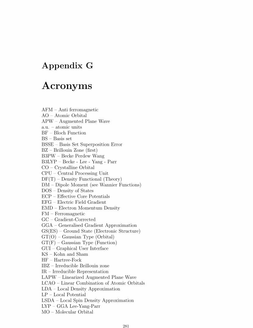
Appendix G

Acronyms

AFM – Anti ferromagneticAO – Atomic OrbitalAPW – Augmented Plane Wavea.u. – atomic unitsBF – Bloch FunctionBS – Basis setBSSE – Basis Set Superposition ErrorBZ – Brillouin Zone (first)B3PW – Becke Perdew WangB3LYP – Becke - Lee - Yang - ParrCO – Crystalline OrbitalCPU – Central Processing UnitDF(T) – Density Functional (Theory)DM – Dipole Moment (see Wannier Functions)DOS – Density of StatesECP – Effective Core PotentialsEFG – Electric Field GradientEMD – Electron Momentum DensityFM – FerromagneticGC – Gradient-CorrectedGGA – Generalised Gradient ApproximationGS(ES) – Ground State (Electronic Structure)GT(O) – Gaussian Type (Orbital)GT(F) – Gaussian Type (Function)GUI – Graphical User InterfaceKS – Kohn and ShamHF – Hartree-FockIBZ – Irreducible Brillouin zoneIR – Irreducible RepresentationLAPW – Linearized Augmented Plane WaveLCAO – Linear Combination of Atomic OrbitalsLDA – Local Density ApproximationLP – Local PotentialLSDA – Local Spin Density ApproximationLYP – GGA Lee-Yang-ParrMO – Molecular Orbital

281

MPP – Massive Parallel ProcessorMSI – Molecular Simulation Inc.NLP – Non-local potential (correlation)PBE – GGA Perdew-Burke-ErnzerhofPDOS – Projected Density of StatesPP – PseudopotentialPVM – Parallel Virtual MachinePW – Plane WavePWGGA – GGA. Perdew-WangPWLSD – LSD Perdew-WangPZ – Perdew-ZungerP86 – GGA Perdew 86P91 – Perdew 91QM – Quantum MechanicsRCEP – Relativistic Compact Effective PotentialRHF – Restricted Hartree-FockROHF – Restricted Open-shell Hartree-FockSAED – Symmetry Allowed Elastic DistortionsSABF – Symmetry Adapted Bloch Functions SC – SupercellSCF – Self-Consistent-FieldSTO – Slater Type OrbitalUHF – Unrestricted Hartree-FockVBH – von Barth-HedinVWN – Vosko-Wilk-NusairWnF – Wannier Functions 0D – no translational symmetry1D – translational symmetry in 1 direction (x, CRYSTAL convention)2D – translational symmetry in 2 directions (x,y, CRYSTAL convention)3D – translational symmetry in 3 directions (x,y,z CRYSTAL convention)

282

Bibliography

[1] M. Abramovitz and I. Segun, editors. Handbook of Mathematical Functions.Dover, New York, 1965.

[2] C. Adamo and V. Barone. Toward reliable density functional methodswithout adjustable parameters: the pbe0 model. J. Chem. Phys., 110:6158–6170, 1999.

[3] D. G. Anderson. J. Assoc. Comput. Mach., 12:547, 1964.

[4] E. Apra. Metodi quanto-meccanici per lo studio di solidi cristallini. PhDthesis, University of Torino, Torino, 1993.

[5] T. Asthalter, W. Weyrich, A.H. Harker, A.B. Kunz, R. Orlando, andC. Pisani. Comparison of quasi-hartree-fock wave-functions for lithiumhydride. Solid State Comm., 83:725, 1992.

[6] A. Veillard B. Roos, C. Salez and E. Clementi. A general program forcalculation of atomic SCF orbitals by the expansion method. Tech. Rep.RJ518 IBM Res., 1968.

[7] E. B. Barrosa, A. Joriob, G. G. Samsonidzef, R. B. Capazc, A. G. SouzaFilhoa, J. Mendes Filhoa, G. Dresselhause, and M. S. Dresselhaus. Re-view on the symmetry-related properties of carbon nanotubes. Phys. Rep.,431:261–302 (and references therein), 2006.

[8] J.C. Barthelat. Private communication.

[9] J.C. Barthelat and P. Durand. Gazz. Chim. Ital., 108:225, 1978.

[10] J.C. Barthelat, P. Durand, and A. Serafini. Molec. Phys., 33:159, 1977.

[11] A. D. Becke. J. Chem. Phys., 88:2547, 1988.

[12] A. D. Becke. J. Chem. Phys., 88:1053, 1988.

[13] A. D. Becke. Density-functional exchange-energy approximation with cor-rect asymptotic behavior. Phys. Rev. A, 38:3098–3100, 1988.

[14] A. D. Becke. Density-functional thermochemistry. iii the role of exact ex-change. J. Chem. Phys., 98:5648, 1993.

[15] J.S. Binkley, J.A. Pople, and W.J. Hehre. J. Am. Chem. Soc., 102:939,1980.

[16] Y. Bouteiller, C. Mijoule, M. Nizam, J.C. Barthelat, J.P. Daudey, M. Pel-lissier, and B. Silvi. Mol. Phys., 65:295, 1988.

283

[17] S.F. Boys and F. Bernardi. The calculation of small molecular interactionby the difference of separate total energies. some procedures with reducederrors. Mol. Phys., 19:553, 1970.

[18] C. G. Broyden. Math. Comput., 19:577, 1965.

[19] C.G. Broyden. The convergence of a class of double-rank minimizationalgorithms 1. general considerations. IMA J. Appl. Math., 6:76–90, 1970.

[20] C.G. Broyden. The convergence of a class of double-rank minimizationalgorithms 1. the new algorithm. IMA J. Appl. Math., 6:222–231, 1970.

[21] H. Burzlaff and A. Hountas. J. Appl. Cryst., 15:464, 1982.

[22] S. Casassa, C. M. Zicovich-Wilson, and C. Pisani. Symmetry-adapted lo-calized wannier functions suitable for periodic calculations. Theor. Chem.Acc., 116:726–733, 2006.

[23] M. Catti, R. Dovesi, A. Pavese, and V. R. Saunders. Elastic constants andelectronic structure of fluorite (caf2): an ab initio hartree-fock study. J.Phys.: Condens. Matter, 3:4151, 1991.

[24] M. Causa, R. Dovesi, R. Orlando, C. Pisani, and V.R. Saunders. Treatmentof the exchange interactions in hartree-fock lcao calculations of periodicsystems. J. Phys. Chem., 92:909, 1988.

[25] M. Causa, R. Dovesi, C. Pisani, and C. Roetti. Electronic structure andstability of different crystal phases of magnesium oxide. Phys. Rev. B,33:1308, 1986.

[26] M. Causa, R. Dovesi, and C. Roetti. Pseudopotential hartree-fock studyof seventeen iii-v and iv-iv semiconductors. Phys. Rev. B, 43:11937, 1991.

[27] B. Civalleri, C. M. Zicovich-Wilson, L. Valenzano, and P. Ugliengo. B3lypaugmented with an empirical dispersion term (b3lyp-d*) as applied tomolecular crystal. Crys. Eng. Comm., 10:405–410, 2008.

[28] B. Civalleri, C. M. Zicovich-Wilson, L. Valenzano, and P. Ugliengo. Erratacorrige to: b3lyp augmented with an empirical dispersion term (b3lyp-d*)as applied to molecular crystals. cryst. eng. comm., 10, 405-410 (2008).Cryst. Eng. Comm., 10:1693–1694, 2008.

[29] E. Clementi. MOTECC 91. ESCON, Leiden, 1991.

[30] S. Dall’Olio, R. Dovesi, and R. Resta. Spontaneous polarization as a berryphase of the hartree-fock wave function: the case of knbo3. Phys. Rev.,B56:10105–10114, 1997.

[31] P. D’Arco, Y. Noel, R. Demichelis, and R. Dovesi. Single-layered chrysotilenanotubes: A quantum mechanical ab initio simulation. J. Chem. Phys.,131:Art. N. 204701, 2009.

[32] C. Darrigan, M. Rerat, G. Mallia, and R. Dovesi. Implementation of thefinite field perturbation method in the crystal program for calculating thedielectric constant of periodic systems. J. Comp. Chem., 24:1305–1312,2003.

284

[33] R. Demichelis, Y. Noel, P. D’Arco, and R. Dovesi. Structure and energeticsof imogolite: a quantum mechanical ab initio study with the CRYSTALcode. 2010.

[34] P. A. M. Dirac. Proc. Cambridge Phil. Soc., 26:376, 1930.

[35] R. Dovesi. On the role of symmetry in the ab initio hartree-fock linear com-bination of atomic orbitals treatment of periodic systems. Int. J. QuantumChem., 29:1755, 1986.

[36] R. Dovesi, M. Causa, R. Orlando, C. Roetti, and V.R. Saunders. Ab initioapproach to molecular crystals: a periodic hartree-fock study of crystallineurea. J. Chem. Phys., 92:7402, 1990.

[37] R. Dovesi, E. Ferrero, C. Pisani, and C. Roetti. Ab initio study of theelectron momentum distribution of metallic lithium. Z. Phys. B, 51:195,1983.

[38] R. Dovesi and R. Orlando. Convergence properties of the supercell ap-proach in the study of local defects in solids. Phase Trans., 52:151, 1994.

[39] R. Dovesi, C. Pisani, C. Roetti, M. Causa, and V.R. Saunders. CRYS-TAL88, An ab initio all-electron LCAO-Hartree-Fock program for periodicsystems. QCPE Pgm N.577. Quantum Chemistry Program Exchange, In-diana University, Bloomington, Indiana, 1989.

[40] R. Dovesi, C. Pisani, C. Roetti, and V.R. Saunders. Treatment of coulombinteractions in hartree-fock calculations of periodic systems. Phys. Rev. B,28:5781, 1983.

[41] R. Dovesi, C. Roetti, C. Freyria Fava, M. Prencipe, and V.R. Saunders. Onthe elastic properties of lithium, sodium an potassium oxide. an ab initiostudy. Chem. Phys., 156:11, 1991.

[42] R. Dovesi, C. Roetti, and V.R. Saunders. CRYSTAL92 User’s Manual.Universita di Torino and SERC Daresbury Laboratory, 1992.

[43] R. Dovesi, V.R. Saunders, C. Roetti, M. Causa, N. M. Harrison, R. Or-lando, and E. Apra. CRYSTAL95 User’s Manual. Universita di Torino,1996.

[44] R. Dovesi, V.R. Saunders, C. Roetti, R. Orlando, C.M. Zicovich-Wilson,F. Pascale, B. Civalleri, K. Doll, N.M. Harrison, I.J. Bush, Ph. DArco, andM. Llunell. CRYSTAL06 User’s Manual. Universita di Torino, Torino,2006.

[45] P. Durand and J.C. Barthelat. Theor. Chim. Acta, 38:283, 1975.

[46] V.R. Saunders et al. Electronic structure theory: from molecules to crystals.private communication, 1999.

[47] M. Ferrero, M. Rerat, R. Orlando, and R. Dovesi. The calculation ofstatic polarizabilities in 1-3d periodic compounds. the implementation inthe crystal code. J. Comput. Chem., 29:1450–1459, 2008.

285

[48] M. Ferrero, M. Rerat, R. Orlando, and R. Dovesi. Coupled perturbedhartree-fock for periodic systems: the role of symmetry and related com-putational aspects. J. Chem. Phys., 128:Art. N. 014100, 2008.

[49] M. Ferrero, M. Rerat, R. Orlando, R. Dovesi, and I. J. Bush. coupledperturbed kohn-sham calculation of static polarizabilities of periodic com-pounds. J. Phys.: Conf. Ser., 117:Art. N. 012016, 2008.

[50] R. Fletcher. Comput. J, 13:317, 1970.

[51] M. J. Frisch, G. W. Trucks, H. B. Schlegel, G. E. Scuseria, M. A. Robb,J. R. Cheeseman, J. A. Montgomery, Jr., T. Vreven, K. N. Kudin, J. C.Burant, J. M. Millam, S. S. Iyengar, J. Tomasi, V. Barone, B. Mennucci,M. Cossi, G. Scalmani, N. Rega, G. A. Petersson, H. Nakatsuji, M. Hada,M. Ehara, K. Toyota, R. Fukuda, J. Hasegawa, M. Ishida, T. Nakajima,Y. Honda, O. Kitao, H. Nakai, M. Klene, X. Li, J. E. Knox, H. P. Hratchian,J. B. Cross, V. Bakken, C. Adamo, J. Jaramillo, R. Gomperts, R. E. Strat-mann, O. Yazyev, A. J. Austin, R. Cammi, C. Pomelli, J. W. Ochterski,P. Y. Ayala, K. Morokuma, G. A. Voth, P. Salvador, J. J. Dannenberg,V. G. Zakrzewski, S. Dapprich, A. D. Daniels, M. C. Strain, O. Farkas,D. K. Malick, A. D. Rabuck, K. Raghavachari, J. B. Foresman, J. V. Or-tiz, Q. Cui, A. G. Baboul, S. Clifford, J. Cioslowski, B. B. Stefanov, G. Liu,A. Liashenko, P. Piskorz, I. Komaromi, R. L. Martin, D. J. Fox, T. Keith,M. A. Al-Laham, C. Y. Peng, A. Nanayakkara, M. Challacombe, P. M. W.Gill, B. Johnson, W. Chen, M. W. Wong, C. Gonzalez, , and J. A. Pople.Gaussian 03, Revision 02. Gaussian, Inc., Wallingford CT, 2004, 2004.

[52] M. J. Frisch, G. W. Trucks, H. B. Schlegel, G. E. Scuseria, M. A. Robb,J. R. Cheeseman, V. G. Zakrzewski, J. A. Montgomery, Jr., R. E. Strat-mann, J. C. Burant, S. Dapprich, J. M. Millam, A. D. Daniels, K. N.Kudin, M. C. Strain, O. Farkas, J. Tomasi, V. Barone, M. Cossi, R. Cammi,B. Mennucci, C. Pomelli, C. Adamo, S. Clifford, J. Ochterski, G. A. Pe-tersson, P. Y. Ayala, Q. Cui, K. Morokuma, D. K. Malick, A. D. Rabuck,K. Raghavachari, J. B. Foresman, J. Cioslowski, J. V. Ortiz, B. B. Ste-fanov, G. Liu, A. Liashenko, P. Piskorz, I. Komaromi, R. Gomperts, R. L.Martin, D. J. Fox, T. Keith, M. A. Al-Laham, C. Y. Peng, A. Nanayakkara,C. Gonzalez, M. Challacombe, P. M. W. Gill, B. Johnson, W. Chen, M. W.Wong, J. L. Andres, C. Gonzalez, M. Head-Gordon, E. S. Replogle, andJ. A. Pople. Gaussian 98, Revision A.3. Pittsburgh PA, 1998.

[53] M.J. Frisch, G.W. Trucks, H.B. Schlegel, P.M.W. Gill, B.G. Johnson,M.A. Robb, J.R. Cheeseman, T.A. Keith, G.A. Pettersson, J.A. Mont-gomery, K. Raghavachari, M.A. Al-Laham, V.G. Zakrzewski, J.V. Ortiz,J.B. Foresman, J. Cioslowski, B.B. Stefanov, A. Nanayakkara, M. Challa-combe, C.Y. Peng, P.Y. Ayala, W. Chen, M.W. Wong, J.L. Andres, E.S.Replogle, R. Gomperts, R.L. Martin, D.J. Fox, J.S. Binkley, D.J. Defrees,J. Baker, J.J.P. Stewart, M. Head-Gordon, C. Gonzalez, , and J.A. Pople.Gaussian 94 (Revision A.I). Gaussian Inc., Pittsburgh PA, 1995.

[54] L. Fu, E. Yaschenko, L. Resca, and R. Resta. Hartree–fock approachto macroscopic polarisation: Dielectric constant and dynamical charge ofknbo3. Phys. Rev. B, 57:6967–6971, 1988.

286

[55] C. Giacovazzo. Fundamentals of Crystallography. IUC-Oxford UniversityPress, Oxford, 1992.

[56] G. Gilat. J. Comp. Phys., 10:432, 1972.

[57] G. Gilat and L.J. Raubenheimer. Accurate numerical method for calculat-ing frequency-distribution in solids. Phys. Rev., 144:390, 1966.

[58] P.M.W. Gill, B.G. Johnson, and J.A. Pople. A standard grid for densityfunction calculations. Chem. Phys. Lett., 209:506–512, 1993.

[59] D. Goldfarb. Math. Comput., 24:23, 1970.

[60] M.S. Gordon, J.S. Binkley, J.A. Pople, W.J. Pietro, and W.J. Hehre.J. Am. Chem. Soc., 104:2797, 1982.

[61] S. Grimme. Semiempirical gga-type density functional constructed with along range dispersion correction. J. Comput. Chem, 27:1787–, 2006.

[62] M.F. Guest and V.R. Saunders. On methods for converging open-shellhartree-fock wave-functions. Mol. Phys., 28:819–828, 1974.

[63] G. Igel-Mann H. Stoll and H. Preuss. Arbeitsbericht 27 des Instituts furTheoretische Chemie, Universitat Stuttgart, 1990.

[64] T. Hahn. International Tables for Crystallography. Reidel Publishing Com-pany, 1987.

[65] D. R. Hamann. Semiconductor charge densities with hard-core and soft-core pseudopotentials. Phys. Rev. Lett., 42:662–665, 1979.

[66] P.C. Hariharan and J.A. Pople. Theor. Chim. Acta, 28:213, 1973.

[67] P.J. Hay and W.R. Wadt. Ab initio effective core potentials for molec-ular calculations. potentials for k to au including the outermost orbitals.J. Chem. Phys., 82:299, 1985.

[68] P.J. Hay and W.R. Wadt. Ab initio effective core potentials for molecularcalculations. potentials for main group elements na to bi. J. Chem. Phys.,82:284, 1985.

[69] P.J. Hay and W.R. Wadt. Ab initio effective core potentials for molecularcalculations. potentials for transition metal atoms sc to hg. J. Chem. Phys.,82:270, 1985.

[70] D.J. Hehre, W.A. Lathan, M.D. Newton, R. Ditchfield, and J.A.Pople. GAUSSIAN70 Program number 236, QCPE. Indiana Univer-sity,Bloomington, Indiana, 1972.

[71] D.J. Hehre, L. Radom, P.v.R. Schleyer, and J.A. Pople. Ab initio molecularorbital theory. Wiley, New York, 1986.

[72] W.J. Hehre, R. Ditchfield, R.F. Stewart, and J.A. Pople. J. Chem. Phys.,52:2769, 1970.

[73] W.J. Hehre, R.F. Stewart, and J.A. Pople. J. Chem. Phys., 51:2657, 1969.

287

[74] P Hohenberg and W. Kohn. Inhomogeneous electron gas. Phys. Rev.,136:B864, 1964.

[75] D. D. Johnson. Modified broyden’s method for accelerating convergence inself-consistent calculations. Phys. Rev B, 38:12807–12813, 1988.

[76] W. Kohn and L.J. Sham. Self-consistent equations including exchange andcorrelation effects. Phys. Rev., 140:A1133, 1965.

[77] L. Kronsjo. Algorithms, their complexity and efficiency, volume 2nd ed.Wiley, New York, 1986.

[78] C. Lee, W. Yang, , and R. G. Parr. Development of the colle-salvetticorrelation-energy formula into a functional of the electron density. Phys.Rev. B, 37:785–789, 1988.

[79] K.H. Lee, M. Causa, and S.S. Park. Ab initio periodic hartree-fock calcula-tions for interpretation of the scanning tunneling microscope (stm) imagesof graphite. J. Phys. Chem. B, 102:6020, 1998.

[80] B. Lindberg. J. Chem. Phys., 88:3805–xxxx, 1988.

[81] R. Lindh, A. Bernhardsson, G. Katlstrom, and P.A. Malmqvist. On the useof a hessian model function in molecular geometry optimizations. Chem.Phys. Letters, 241:423–428, 1995.

[82] V. Magnasco and A. Perico. J. Chem. Phys., 47:971, 1967.

[83] N.D. Mermin. Thermal properties of the inhomogeneous electron gas. Phys.Rev. A, 137:1441, 1965.

[84] D. Moncrieff and V.R. Saunders. Atmol. University of Manchester RegionalComputing Centre, Doc NAT648, 1986.

[85] H.J. Monkhorst and J.D. Pack. Phys. Rev., 13:5188, 1976.

[86] R. Orlando, R. Dovesi, C. Roetti, and V.R. Saunders. Ab initio hartree-fock calculations of periodic compounds: application to semiconductors. J.Phys. Condens. Matter, 2:7769, 1990.

[87] D. Viterbo P. Ugliengo and G. Chiari. Moldraw: Molecular graphics on apersonal computer. Zeitschrift fur Kristallographie, 207:9, 1993.

[88] J. P. Perdew. Density-functional approximation for the correlation energyof the inhomogeneous electron gas. Phys. Rev. B, 33:8822, 1986.

[89] J. P. Perdew. Electronic Structure of Solids 1991. Akademie Verlag, Berlin,1991.

[90] J. P. Perdew, K. Burke, and M. Ernzerhof. Generalized gradient approxi-mation made simple. Phys. Rev. Lett., 77:3865–3868, 1996.

[91] J. P. Perdew and Y. Wang. Accurate and simple analytic representationof the electron gas correlation energy. Phys. Rev. B, 45:13244, 1992.

[92] J. P. Perdew and Wang Yue. Accurate and simple density functionalfor the electronic exchange energy: Generalized gradient approximation.Phys. Rev. B, 33:8800–8802, 1986.

288

[93] J. P. Perdew and Wang Yue. Erratum: Accurate and simple density func-tional for the electronic exchange energy: Generalized gradient approxima-tion. Phys. Rev. B, 40:3399, 1989.

[94] J. P. Perdew and A. Zunger. Self-interaction correction to density-functional approximations for many-electron systems. Phys. Rev. B,23:5048–5079, 1981.

[95] J.P. Perdew, J.A. Chevary, S.H. Vosko, K.A. Jackson, M.R. Pederson, D.J.Singh, and C. Fiolhais. Atoms, molecules, solids and surfaces: applicationsof the generalized gradient approximation for exchange and correlation.Phys. Rev. B, 46:6671, 1992.

[96] J.P. Perdew, A. Ruzsinszky, G.I. Csonka, O.A. Vydrov, G.E. Scuseria, L.A.Constantin, X. Zhou, and K. Burke. Phys. Rev. Letters, 100:Art. N. 184109,2008.

[97] W.J. Pietro, E.S. Blurock, R.F. Hout, W.J. Hehre, W.J. DeFrees, and R.F.Stewart. Inorg. Chem., 20:3650, 1981.

[98] W.J. Pietro, B.A. Levi, W.J. Hehre, and R.F. Stewart. Inorg. Chem.,19:2225, 1980.

[99] J. Pipek and P. G. Mezey. J. Chem. Phys., page 4916, 1989.

[100] C. Pisani. Quantum-mechanical ab-initio calculation of the properties ofcrystalline materials. volume 67 of Lecture Notes in Chemistry, Berlin,1996. Springer Verlag.

[101] C. Pisani, E. Apra, , and M. Causa. Density matrix of crystalline systems.i. long range behavior and related computational problems. Int. J. Quan-tum Chem., 38:395, 1990.

[102] C. Pisani, E. Apra, M. Causa, and R. Orlando. Density matrix of crystallinesystems. ii. the influence of structural and computational parameters. Int.J. Quantum Chem., 38:419, 1990.

[103] C. Pisani, R. Dovesi, and C. Roetti. Hartree-Fock ab initio Treatment ofCrystalline Systems, volume 48 of Lecture Notes in Chemistry. SpringerVerlag, Heidelberg, 1988.

[104] J.A Pople and R.K. Nesbet. Self-consistent orbitals for radicals.J. Chem. Phys., 22:571, 1954.

[105] M.J.D Powell, editor. Academic Press, New York, 1982.

[106] M. Rerat, M. Ferrero, E. Amzallag, I. Baraille, and R. Doveesi. Comparisonof the polarizability of periodic systems computed by using the length andvelocity operators. J. Phys.: Conf. Ser., 117:Art. N. 012023, 2008.

[107] R. Resta. The geometric phase approach to macroscopic polarization incrystalline dielectrics. Rev. Mod. Phys., 66:809, 1994.

[108] C.C.J. Roothaan. Self-consistent field theory for open shells of electronicsystems. Rev. Mod. Phys., 32:179–185, 1960.

289

[109] L. Salasco, R. Dovesi, R. Orlando, C. Pisani, M. Causa, and V.R. Saunders.A periodic ab initio extended basis set study of α-al2o3. Mol. Phys., 72:267,1992.

[110] V. R. Saunders. From molecules to solids. Book in preparation.

[111] V.R. Saunders. Ab initio hartree-fock calculations for periodic systems.Faraday Symp. Chem. Soc., 19:79–84, 1984.

[112] V.R. Saunders, R. Dovesi, C. Roetti, M. Causa, N. M. Harrison, R. Or-lando, and C.M. Zicovich-Wilson. CRYSTAL98 User’s Manual. Universitadi Torino, Torino,1998.

[113] V.R. Saunders, R. Dovesi, C. Roetti, R. Orlando, C.M. Zicovich-Wilson,N. M. Harrison, K. Doll, B. Civalleri, I. Bush, Ph. D’Arco, and M. Llunell.CRYSTAL03 User’s Manual. Universita di Torino, Torino,2003.

[114] V.R. Saunders, C. Freyria-Fava, R. Dovesi, L. Salasco, and C. Roetti. Onthe electrostatic potential in crystalline systems where the charge densityis expanded in gaussian functions. Mol. Phys., 77:629, 1992.

[115] A. Savin. Int. J. Quantum Chem., S22:457, 1988.

[116] G. Schaftenaar. MOLDEN a pre- and post processing program of molecularand electronic structure. CMBI, the Netherlands.

[117] H. B. Schlegel. Optimization of equilibrium and transition structures. J.Comp. Chem., 3:214–218, 1982.

[118] H.B. Schlegel. Estimating the hessian for gradient-type geometry optimiza-tions. Theoret. Chim. Acta, 66:333–340, 1984.

[119] B.G. Searle. Dl visualize. Comp. Phys. Communications, 137:25–32, 2001.

[120] D.F. Shanno. Math. Comput., 24:647, 1970.

[121] W.J. Stevens, H. Bash, and M. Krauss. Compact effective potentials andefficient shared-exponent basis sets for the first- and second-row atoms. J.Chem. Phys, 81:6026–6033, 1984.

[122] W.J. Stevens, M. Krauss, H. Basch, and P.G. Jasien. Relativistic compacteffective potentials and efficient, shared-exponent basis sets for the third-,fourth-, and fifth-row atoms. Can. J. Chem, 70:612–630, 1992.

[123] J. Tersoff and D.R. Hamann. Theory of scanning tunneling microscope.Phys. Rev. B, 31:805, 1985.

[124] M.D. Towler, A. Zupan, and M. Causa. Density functional theory in pe-riodic systems using local gaussian basis sets. Comp. Phys. Commun.,98:181–205, 1996.

[125] O. Treutler and R. Ahlrichs. Efficient molecular numerical integrationschemes. J. Chem. Phys., 102:346–354, 1995.

290

[126] P. Ugliengo, C.M. Zicovich-Wilson, S. Tosoni S, and B. Civalleri. Role ofdispersive interactions in layered materials: a periodic b3lyp and b3lyp-d*study of mg(oh)2, ca(oh)2 and kaolinite. J. Mater. Chem., 19:2564–2572,2009.

[127] U. von Barth and L. Hedin. J. Phys. C: Solid State Phys., 5:1629, 1972.

[128] S. H. Vosko, L. Wilk, and M. Nusair. Accurate spin-dependent electronliquid correlation energies for local spin density calculations: a critical anal-ysis. Can. J. Phys., 58:1200, 1980.

[129] R. Dovesi V.R. Saunders, C. Freyria-Fava and C. Roetti. On the electro-static potential in linear periodic polymers. Comp. Phys. Comm., 84:156,1993.

[130] R. C. Weast, M. J. Astle, and W. H. Beyer, editors. CRC Handbook ofChemistry and Physics, pages A–61 and A–62. CRC Press, Inc., BocaRaton, Florida, 1986-87.

[131] J.A. Weil, J.R. Bolton, and E. Wertz. Electron ParamagneticResonance- Elementary Theory and Practical Applications. John Wiley, New York,1994.

[132] C. T. White, D. H. Robertson, and J. W. Mintmire. Helical and rotationalsymmetries of nanoscale graphitic tubules. Phys. Rev. B, 47:5485–5488,1993.

[133] L.C. Wilson and M. Levy. Nonlocal wigner-like correlation-energy densityfunctional through coordinate scaling. Phys. Rev. B, 41:12930–12932, 1990.

[134] J.M. Wittbrodt and H.B. Schlegel. Estimating stretching force constantsfor geometry optimization. J. Mol. Structure - Theochem, 398-399:55–61,1997.

[135] Zhigang Wu and R.E. Cohen. More accurate generalized gradient approx-imation for solids. Phys. Rev. B, 73:Art. n. 235116, 2006.

[136] Y. Zhang and D.G. Truhlar. J. Chem. Phys., 128:Art. N. 184109, 2008.

[137] C. Zicovich-Wilson and R. Dovesi. On the use of symmetry adapted crys-talline orbitals in scf-lcao p eriodic calculations.ii. implementation of the self-consistent-field scheme and examples. Int. J.Quantum Chem., 67:311–320, 1998.

[138] C. Zicovich-Wilson and R. Dovesi. On the use of symmetry adapted crys-talline orbitals in scf-lcao periodic calculations.i. the construction of the symmetrized orbitals. Int. J. Quantum Chem,67:299–310, 1998.

[139] C. M. Zicovich-Wilson and R. Dovesi. Localized functions in crystallinesystems and their variational manifolds. Beyond standard Quantum Chem-istry: From molecules to extended systems, page Chapter 8, India, 2007.Transworld Research Network.

291

[140] C.M. Zicovich-Wilson, R. Dovesi, and V.R. Saunders. A general methodto obtain well localized wannier functions for composite energy bands inlcao periodic calculations. J. Chem. Phys., 115:9708–9718, 2001.

292

Index

ADFT see EDFTNEWBASIS, 154

ALLOWTRUSTR(OPTGEOM), 111ALL(ANISOTRO), 155ANALYSIS(FREQCALC), 128ANBD, 154ANDERSON, 71ANGLES, 30ANGROT(ROTCRY), 54ANGSFROZEN(OPTGEOM), 120ANGSTROM, 31, 155ANGTODOUBLE(OPTGEOM), 115ANGULAR(DFT), 78ANGULAR(EDFT), 154, 164ANHARM, 141

END, 141ISOTOPES, 142KEEPSYMM, 142NOGUESS, 142POINTS26, 142PRINTALL, 142PRINT, 142TEST[ANHA], 142

ANISOTROALL, 155PRINT, 155SELECT, 155UNIQUE, 155

ATOMBSSE, 31ATOMDISP, 32ATOMHF, 72ATOMINSE, 32ATOMIRR, 155ATOMORDE, 32ATOMREMO, 32ATOMROT, 33ATOMSPIN, 72ATOMSUBS, 34ATOMSYMM, 34, 62, 155ATOMS(EIGSHROT), 82ATOMS(MAPNET), 176

AUTO(ROTCRY), 54B3LYP(DFT), 76B3PW(DFT), 76BANDLIST(LOCALWF), 168BAND, 156BARTHE, 65BASE(FIXINDEX), 86BASISSET, 156BATCHPNT(DFT), 80BECKE(DFT), 75, 77BECKE(EDFT), 154, 164BERNY(OPTGEOM), 110BETALOCK, 73BFGS(OPTGEOM), 110BIDIERD, 157

CONV, 157DIFF, 157DIR, 157END, 157PROF, 157

BIESPLIT, 73BIPOLAR, 73BIPOSIZE, 73BOHRANGS, 34BOHRCR98, 34BOHR, 34, 157BOYSCTRL(LOCALWF, 170BREAKELAS, 35BREAKSYM, 26, 34BROYDEN, 73BR(PROF), 185BUNITSDECO(FREQCALC), 131BWIDTH, 158CAPTURE(LOCALWF), 171CELLONLY(OPTGEOM), 109CHARGED, 62, 158CHARGE (GRID3D), 166CHEMOD, 62CHNGTSFOL(OPTGEOM), 124CHUNKS(DFT), 81CLAS, 158

293

CLUSPLUS(LOCALWF), 173CLUSTER, 36CMPLXFAC, 104CONFCNT, 146CONV(BIDIERD), 157CONV(PROF), 185COORDINA(MAPNET) , 176COORPRT, 37, 158CORRELAT(DFT), 74CPHF, 144

END, 144MAXCYCLE, 144RESTART, 144TOLALPHA, 144TOLUDIK, 144

CP(PROF), 185CRYAPI OUT, 159CRYDEF(OPTGEOM), 112CRYSTAL, 13CVOLOPT(OPTGEOM), 117CYCTOL(LOCALWF), 169DBANGLIST(OPTGEOM), 116DCDIAG, 104DEFANGLS(OPTGEOM), 116DEFLNGS(OPTGEOM), 116DENSMAT, 158DFT

ANGULAR, 78B3LYP, 76B3PW, 76BATCHPNT, 80BECKE, 75, 77CHUNKS, 81CORRELAT, 74DISTGRID, 79END[DFT], 74EXCHANGE, 75FCHARGE, 81HYBRID, 76LDA, 75LGRID, 78LYP, 75NEWTON, 81NONLOCAL, 76PB86, 75PBE0, 76PBESOL, 75PBE, 75PWGGA, 75

PWLSD, 75PZ, 75RADIAL, 78RADIUS, 81REPLGRID, 80SAVIN, 77SOGGAXC, 76SOGGA, 75SPIN, 75TOLLDENS, 80TOLLGRID, 80VBH, 75VWN, 75WCGGA, 75WL, 75XLGRID, 79XXLGRID, 79

DIELISO(FREQCALC), 128DIELTENS(FREQCALC), 128DIEL/DIELECT, 159DIFF(BIDIERD), 157DIFF(PROF), 185DIPOMOME(FREQCALC), 134DIR(BIDIERD), 157DISPERSION(FREQCALC), 143DISTGRID(DFT), 79DLVINPUT, 15DOSS, 161DURAND, 65ECH3, 162

RANGE, 162SCALE, 162

ECHG, 163EDFT, 163

ANGULAR, 154, 164BECKE, 154, 164PRINTOUT, 154, 164PRINT, 154, 164RADIAL, 154, 164SAVIN, 154, 164

EIGSHIFT, 82EIGSHROT, 82

ATOMS, 82MATRIX, 82

EIGS, 81ELASTCON, 148

END, 148NUMDERIV, 148PREOPTGEOM, 148

294

PRINT, 148RESTART, 148STEPSIZE, 148

ELASTIC, 38EMDLPG, 165EMDL, 164EMDP, 165END

DFT, 74ENDB basis set input, 63ENDG geometry input, 39general information input, 74properties input, 166

END(ANHARM), 141END(BIDIERD), 157END(CPHF), 144END(ELASTCON), 148END(EOS), 39END(FREQCALC), 127END(OPTGEOM), 105END(PROF), 185END(SYMMWF), 171EOS, 39

END, 39PREOPTGEOM, 39PRINT, 39RANGE, 39RESTART, 39

EXCHANGE(DFT), 75EXCHGENE, 83EXCHSIZE, 83EXPDE(OPTGEOM), 112EXTERNAL, 15, 263EXTPRESS(OPTGEOM), 121EXTPRT, 41, 166EXTSTRESS(OPTGEOM), 121FCHARGE(DFT), 81FDAOSYM, 83FDOCCUP, 84FIELDCON, 43FIELD, 41FINALRUN (OPTGEOM), 112, 209FINDSYM, 44FITDEGR(OPTGEOM), 113FITTOPATH(OPTGEOM), 124FIXCELL(OPTGEOM), 116FIXCOOR(OPTGEOM), 119FIXDEF(OPTGEOM), 118FIXDEIND(OPTGEOM), 112

FIXDELTE(OPTGEOM), 112FIXDELTX(OPTGEOM), 112FIXINDEX, 86

BASE, 86GEBA, 86GEOM, 86

FMIXING, 87FMWF, 166FRACTCOOR(OPTGEOM), 112FRACTION, 166

geometry input, 44FRACTION(OPTGEOM), 112FRACTIOO(OPTGEOM), 112FRAGMENT(FREQCALC), 128FRAGMENT(OPTGEOM), 119, 208FREEZDIH(OPTGEOM), 121FREEZINT(OPTGEOM), 120FREQCALC, 126

ANALYSIS, 128BUNITSDECO, 131DIELISO, 128DIELTENS, 128DIPOMOME, 134DISPERSION, 143END, 127FRAGMENT, 128INTENS, 132INTLOC, 133INTPOL, 133ISOTOPES, 128MODES, 130NOANALYSIS, 130NOINTENS, 130NOKSYMDISP, 143NOMODES, 130NOOPTGEOM, 127NORMBORN, 130NOUSESYMM, 130NUMDERIV, 130PREOPTGEOM, 127PRESSURE, 130PRINT, 130REFLECTANCE, 139RESTART, 131SCANMODE, 135STEPSIZE, 131TEMPERAT, 131TEST[FREQ], 131USESYMM, 131

295

FULLBOYS(LOCALWF), 174FULLOPTG(OPTGEOM), 109FULLTIME, 103GAUSS98, 63GEBA(FIXINDEX), 86GEOM(FIXINDEX), 86GHOSTS, 64GRADCAL, 87GRID3D, 166

CHARGE, 166POTENTIAL, 166

GRIMME, 88GUESDUAL, 89GUESSF, 91GUESSPAT, 91GUESSP, GUESSP0, 91HAYWLC, 65HAYWSC, 65HELIX, 13HESEVLIM(OPTGEOM), 113HESSFREQ(OPTGEOM), 109HESSIDEN(OPTGEOM), 109HESSMOD1(OPTGEOM), 109HESSMOD2(OPTGEOM), 109HESSNUM(OPTGEOM), 110HESSOPT(OPTGEOM), 109HYBRID(DFT), 76HYDROSUB, 44IGSSBNDS(LOCALWF), 171IGSSCTRL(LOCALWF), 170IGSSVCTS(LOCALWF), 170INFOGUI, 167INFO see INFOGUI, 167INIFIBND(LOCALWF), 168INPUT(ECP input), 65INTENS(FREQCALC), 132INTGPACK, 92INTLOC(FREQCALC), 133INTPOL(FREQCALC), 133INTREDUN(OPTGEOM), 115ISOTOPES(ANHARM), 142ISOTOPES(FREQCALC), 128ISOTROPIC, 167ITACCONV(OPTGEOM), 113ITATOCEL(OPTGEOM), 109KEEPSYMM, 26, 44KEEPSYMM(ANHARM), 142KNETOUT (obsolete), 168KSYMMPRT, 92

LDA(DFT), 75LEVSHIFT, 92LGRID(DFT), 78LNGSFROZEN(OPTGEOM), 120LOCALWF, 168

BANDLIST, 168BOYSCTRL, 170CAPTURE, 171CLUSPLUS, 173CYCTOL, 169FULLBOYS, 174IGSSBNDS, 171IGSSCTRL, 170IGSSVCTS, 170INIFIBND, 168MAXCYCLE, 170OCCUPIED, 168ORTHNDIR, 174PHASETOL, 169PRINTPLO, 173RESTART, 169SYMMWF, 171VALENCE, 168WANDM, 174

LYP(DFT), 75MAKESAED, 45MAPNET, 176

ATOMS, 176COORDINA, 176MARGINS, 176PRINT, 176RECTANGU, 176

MARGINS(MAPNET), 176MATRIX(EIGSHROT), 82MATROT(ROTCRY), 54MAXCYCLE

scf, 93MAXCYCLE(CPHF), 144MAXCYCLE(LOCALWF), 170MAXCYCLE(OPTGEOM), 113MAXCYCLE(scf), 93MAXITACE(OPTGEOM), 113MAXTRADIUS(OPTGEOM), 111MODEFOLLOW(OPTGEOM), 124MODES(FREQCALC), 130MODISYMM, 45MOLDRAW, 45MOLEBSSE, 45MOLECULE, 13

296

from 3D structure, 46MOLEXP, 46MOLSPLIT, 47MONSPLIT, 93MPP, 93MULPOPAN, 96, 184MYBIPOLA, 94NANOJMOL, 51NANORE, 51NANOTUBE, 47NEGLEFRE

NEGLEFRE, 130NEIGHBOR, 51, 95, 177NEIGHPRT see NEIGHBOR, 51NEWBASIS(ADFT), 154NEWK, 178NEWTON(DFT), 81NOANALYSIS(FREQCALC), 130NOBICOU, 95NOBIPEXC, 95NOBIPOLA, 95NOFMWF, 95NOGUESS(ANHARM), 142NOGUESS(OPTGEOM), 113NOINTENS(FREQCALC), 130NOKSYMDISP(FREQCALC), 143NOMODES(FREQCALC), 130NOMONDIR, 95NONLOCAL(DFT), 76NOOPTGEOM(FREQCALC), 127NOPRINT, 64NORMBORN(FREQCALC), 130NOSHIFT, 52NOSYMADA, 95, 179NOSYMAP(SYMMWF), 171NOSYMMOPS(OPTGEOM), 114NOTRUSTR(OPTGEOM), 111NOUSESYMM(FREQCALC), 130NOXYZ(OPTGEOM), 114NRSTEPS(OPTGEOM), 113NUMDERIV(ELASTCON), 148NUMDERIV(FREQCALC), 130NUMGRALL(OPTGEOM), 114NUMGRATO(OPTGEOM), 114NUMGRCEL(OPTGEOM), 114Nanotube rebuild, 50OCCUPIED(LOCALWF), 168OLDCG(OPTGEOM), 110ONELOG(OPTGEOM), 114

OPTGEOM, 105ALLOWTRUSTR, 111ANGSFROZEN, 120ANGTODOUBLE, 115BERNY, 110BFGS, 110CELLONLY, 109CHNGTSFOL, 124CRYDEF, 112CVOLOPT, 117DBANGLIST, 116DEFANGLS, 116DEFLNGS, 116END, 105EXPDE, 112EXTPRESS, 121EXTSTRESS, 121FINALRUN, 112, 209FITDEGR, 113FITTOPATH, 124FIXCELL, 116FIXCOOR, 119FIXDEF, 118FIXDEIND, 112FIXDELTE, 112FIXDELTX, 112FRACTCOOR, 112FRACTION, 112FRACTIOO, 112FRAGMENT, 119, 208FREEZDIH, 121FREEZINT, 120FULLOPTG, 109HESEVLIM, 113HESSFREQ, 109HESSIDEN, 109HESSMOD1, 109HESSMOD2, 109HESSNUM, 110HESSOPT, 109INTREDUN, 115ITACCONV, 113ITATOCEL, 109LNGSFROZEN, 120MAXCYCLE, 113MAXITACE, 113MAXTRADIUS, 111MODEFOLLOW, 124NOGUESS, 113

297

NOSYMMOPS, 114NOTRUSTR, 111NOXYZ, 114NRSTEPS, 113NUMGRALL, 114NUMGRATO, 114NUMGRCEL, 114OLDCG, 110ONELOG, 114PATHFOLLOW, 124POWELL, 110PRINTFORCES, 114PRINTHESS, 114PRINTOPT, 114PRINT, 114RENOSAED, 112RESTART, 113SORT, 113STEPBMAT, 116STEPSIZE, 114TESTREDU, 117TOLDEE, 110TOLDEG, 110TOLDEX, 110TOLREDU, 117TRUSTRADIUS, 111TSOPT, 123

ORIGIN, 52ORTHNDIR(LOCALWF), 174P86(DFT), 75PARAMPRT, 52, 64, 95, 179PATHFOLLOW(OPTGEOM), 124PATO, 179PBAN, 179PBE0(DFT), 76PBESOL(DFT), 75PBE(DFT), 75PDIBAN see PBAN, 179PDIDE, 180PGEOMW, 180PHASETOL(LOCALWF), 169PHASE, 189PIEZOBP, 188PIEZOWF, 188PMP2, 180POINTCHG, 52POINTS26(ANHARM), 142POLARI, 189POLEORDR, 96

POLI, 181POLSPIN, 181POLYMER, 13POSTSCF, 96POT3, 182

RANGE, 182SCALE, 182

POTC, 183POTENTIAL (GRID3D), 166POTM, 184POWELL(OPTGEOM), 110PPAN, 96, 184PREOPTGEOM(ELASTCON), 148PREOPTGEOM(EOS), 39PREOPTGEOM(FREQCALC), 127PRESSURE(FREQCALC), 130PRIMITIV, 52PRINTALL(ANHARM), 142PRINTCHG, 53PRINTFORCES(OPTGEOM), 114PRINTHESS(OPTGEOM), 114PRINTOPT(OPTGEOM), 114PRINTOUT, 53, 64, 96, 184

ATCOORDS, 255ATOMICWF, 256BASISSET, 256CONFIGAT, 256DFTBASIS, 256DOSS, 256EIGENALL, 256EIGENVAL, 256EIGENVEC, 256ENECYCLE, 256EQUIVAT, 255EXCHGENE, 255FGIRR, 256FGRED, 255GAUSS94, 256GLATTICE, 255KNETOUT, 255KSYMMPRT, 255KWEIGHTS, 255MAPVALUES, 256MULLIKEN, 256MULTIPOL, 256OVERLAP, 255PARAMETERS, 255PGIRR, 255PGRED, 255

298

ROTREF, 256SCALEFAC, 256SYMMOPSR, 255SYMMOPS, 255

PRINTOUT(EDFT), 154, 164PRINTPLO(LOCALWF), 173PRINT (DIEL), 159PRINT(ANHARM), 142PRINT(ANISOTRO), 155PRINT(EDFT), 154, 164PRINT(ELASTCON), 148PRINT(EOS), 39PRINT(FREQCALC), 130PRINT(MAPNET), 176PRINT(OPTGEOM), 114PRINT(SYMMWF), 171PROF, 185

BR, 185CONV, 185CP, 185DIFF, 185END, 185

PROF(BIDIERD), 157PRSYMDIR, 53PSCF, 186PURIFY, 53PWGGA(DFT), 75PWLSD(DFT), 75PZ(DFT), 75QVRSGDIM, 104RADIAL(DFT), 78RADIAL(EDFT), 154, 164RADIUS(DFT), 81RANGE (ECH3), 162RANGE (POT3), 182RANGE(EOS), 39RAYCOV/RAYC/RCOVFACT, 53,

186RDFMWF, 166RECTANGU(MAPNET), 176REDEFINE see SLABINFO, 56REFLANGLE(REFLECTANCE), 140REFLDAMP(REFLECTANCE), 140REFLDIR(REFLECTANCE), 139REFLECTANCE

REFLANGLE, 140REFLDAMP, 140REFLNSTEP, 140REFLRANGE, 140

REFLSTEPS, 140REFLECTANCE(FREQCALC), 139REFLECTANCEREFLDIR, 139REFLNSTEP(REFLECTANCE), 140REFLRANGE(REFLECTANCE), 140REFLSTEPS(REFLECTANCE), 140RENOSAED(OPTGEOM), 112REPLGRID(DFT), 80RESTART(CPHF), 144RESTART(ELASTCON), 148RESTART(EOS), 39RESTART(FREQCALC), 131RESTART(LOCALWF), 169RESTART(OPTGEOM), 113RHF, 96ROTATE see SLABINFO, 56ROTCRY, 54

ANGROT, 54AUTO, 54MATROT, 54

ROTREF, 186SAVEWF, 97SAVIN(DFT), 77SAVIN(EDFT), 154, 164SCALE (ECH3), 162SCALE (POT3), 182SCANMODE(FREQCALC), 135SCELPHONO, 58SCFDIR, 96SELECT(ANISOTRO), 155SETINF, 54, 64, 97, 187SETPRINT, 54, 64, 97, 187SHRINK, 97SLABCUT/SLAB, 55SLABINFO, 56SLAB, 13SMEAR, 99SOGGAXC(DFT), 76SOGGA(DFT), 75SORT(OPTGEOM), 113SPINEDIT, 100SPINLOCK, 101SPIN(DFT), 75SPOLBP, 191SPOLWF, 192STEPBMAT(OPTGEOM), 116STEPSIZE(ELASTCON), 148STEPSIZE(FREQCALC), 131STEPSIZE(OPTGEOM), 114

299

STOP, 56, 65, 101, 187STRUCPRT, 56SUPERCEL, 56SUPERCON, 60SWCNTRE, 51SWCNT, 50SYMADAPT, 101, 187SYMMDIR, 60SYMMOPS, 60, 65SYMMREMO, 60SYMMWF

END, 171NOSYMAP, 171PRINT, 171TOLBOND, 171TOLSYM, 171

SYMMWF(LOCALWF), 171TEMPERAT(FREQCALC), 131TENSOR, 60TESTGEOM, 60TESTPDIM, 101TESTREDU(OPTGEOM), 117TESTRUN, 101TEST[ANHA](ANHARM), 142TEST[FREQ](FREQCALC), 131TEST, 65TOLALPHA(CPHF), 144TOLBOND(SYMMWF), 171TOLDEE, 102TOLDEE(OPTGEOM), 110TOLDEG(OPTGEOM), 110TOLDEP, 102TOLDEX(OPTGEOM), 110TOLINTEG, 102TOLLDENS(DFT), 80TOLLGRID(DFT), 80TOLPSEUD, 102TOLREDU(OPTGEOM), 117TOLSYM(SYMMWF), 171TOLUDIK(CPHF), 144TRASREMO, 60TRUSTRADIUS(OPTGEOM), 111TSOPT(OPTGEOM), 123UHF, 102UNIQUE(ANISOTRO), 155USESAED, 61USESYMM(FREQCALC), 131VALENCE(LOCALWF), 168VBH(DFT), 75

VWN(DFT), 75WANDM(LOCALWF), 174WCGGA(DFT), 75WL(DFT), 75XFAC, 187XLGRID(DFT), 79XXLGRID(DFT), 79ZCOR see EDFT, 1630D systems input, 141D systems input, 142D from 3D, 552D systems input, 143D systems input, 14

adjoined gaussian, 220adsorbed molecule rotation, 33adsorption of molecules, 32Anderson method for accelerating con-

vergence, 71angles printing, 30angular integration (DFT), 78, 154, 164anharmonic calculation, 141anisotropic tensor, 155anisotropy shrinking factor, 24, 99anti ferromagnetic systems, 103Aragonite, 194asymmetric unit, 16ATMOL integral package, 92atomic

density matrix, 72, 179wave function, 72

atomic energy(correlation) a posteriori, 154

atomic number conventional, 18Atomic Orbital

definition, 220order, 21

atomic unitsbohr, 34charge, 181conversion factor, 34

atoms(group of) rotation, 33addition, 32displacement, 32removal, 32reordering, 32substitution, 34

autocorrelation function theory, 226

300

band structure calculation, 156band width, 158BAND.DAT, 259basis set, 214, 220

f and d AO occupation, 84all electron, 19, 20AO symmetry analysis, 83criteria for selection, 214crystal, 20Effective Core Pseudopotential, 67input, 19input examples, 200libraries, 214linear dependence check, 81metals, 217orbital ordering, 21Pople, 19printing, 256printing removed, 64type, 19valence only, 19, 20

basis set superposition errormolecular, 45atomic, 31periodic, 64

Beryllium slab, 197BF - Bloch Functions, 220bi-electronic integrals

indexing, 86bielectronic integrals

file split, 73package, 92

bipolar expansionbielectronic integrals, 73, 94, 224Coulomb buffer, 73coulomb integrals, 95elimination, 95, 224exchange buffer, 83exchange integrals, 95

Bloch Functionsdefinition, 220Symmetry Adapted, 225Symmetry Adapted - printing, 92

Boyslocalization, 168

Bravais lattice, 17, 56, 243Brillouin zone, 221

sampling, 23, 97, 226

Broyden method for accelerating con-vergence, 73

bufferCoulomb bipolar expansion, 73exchange bipolar expansion, 83

bulk modulus, 231BZ - Brillouin Zone, 221

Calcite, 195cell

centred, 18charged, 22conventional, 17conventional/primitive transforma-

tion, 243crystallographic, 17minimum set parameters, 16neutrality, 62non neutral, 62primitive, 17, 52redefinition, 56

Cesium Chloride, 194Chabazite, 196check

basis set input, 101complete input deck, 101disk storage to allocate, 101geometry input, 60

chemisorption, 32Cholesky reduction, 81, 219cluster expansion mapping of CRYS-

TAL calculations, 146cluster from 3D, 36CO - Carbon Monoxide

molecule, 200on MgO (001), 198

CO - Crystalline Orbital, 220Compton profile

average, 227directional, 227input, 185theory, 226

constraint sp, 220contour maps, 176contraction

coefficients, 19of gaussians, 19, 220

conventional atomic number, 18–20conventional cell, 17

301

convergenceacceleration techniques, 24, 99tools

Anderson method, 71Broyden method, 73dual basis, 89Fock/KS matrix mixing, 87level shifter, 92

convergence criteriacycles overflow, 93density matrix, 102

conversion factors, 34length, 34

conversion factors (CR98), 34conversion wave function data, 166coordinates

of equivalent atoms, 18output, 37, 158units, 31

angstrom, 155bohr, 34, 157fraction, 166fractional, 44

units of measure, 14Corundum

(0001) surface, 197(1010) surface, 197bulk, 195

Coulomb energy, 221Coulomb series, 222

bielectronic contribution, 222Coulomb series threshold, 102Coupled Perturbed HF/KS

in a crystal, 144through a slab, 144

covalent radiicustomised, 53, 186default value, 53

Crystalline Orbital (CO)definition, 220

crystallographic cell, 17crystals

(3D) input, 14Cuprite, 194

defectsdisplacement, 32in supercell, 56interstitial, 32

substitutional, 34vacancies, 32

density functionalsee DFT, 74

density matrixatomic, 179band projected, 179behaviour, 223core electrons, 152direct space, 221editing, 100energy projected , 180from geometrical weights, 180initial guess, 91output, 159restore, 186rotation, 186valence electrons, 152

density of statescalculation, 161Fourier-Legendre expansion, 162,

226integrated, 162

DFTfunctionals, 74Hamiltonian, 74input, 74integration scheme, 77

Diamond, 193(100) Surface, 198

DIEL.DAT, 161, 259dielectric constant (optical), 159dielectric tensor, 144dual basis, 89

ECP - see Effective Core Pseudopoten-tial, 65

ECP input examples, 201Edingtonite, 196Effective Core Pseudopotential

input, 65BARTHE, 65DURAND, 65HAYWLC, 65HAYWSC, 65input examples, 201truncation criteria, 102

eigenvalues (Hamiltonian), 220eigenvalues (Hamiltonian) printing, 253

302

eigenvectorscalculation, 178, 220output, 159principal components printout, 154printing, 253printing (core), 254rotation, 186

elastic constant, 38, 228elastic constants, 148elastic distortion, 38elastic moduli theory, 228elastic strain, 228elastic tensor, 229electric field, 184

along non-periodic direction, 43in a crystal, 41through a slab, 41

electric susceptibility, 144electron charge density

3D maps, 162calculation, 163gradient, 163

electron momentum densityline, 164, 165plane, 165theory, 226

electron spin density, 163electronic configuration

ions, 22open shell atoms, 21

electronic properties, 151electrostatic potential

2D maps, 1843D maps, 182first derivative, 183maps, 158second derivative, 183with an electric field, 183

EMD theory, 226energy

(correlation) a posteriori, 163atomic, 22Coulomb, 221exchange (definition), 223exchange contribution, 83Fermi, 221

energy derivatives (elastic constants),228

equation of state, 39

equivalent atoms coordinates, 18exchange energy

calculation, 83theory, 221

exchange series threshold, 102, 223

Faujasite, 196Fermi contact, 167Fermi energy, 221, 226

smear, 99findsym, 26FINDSYM.DAT, 26Fluorite, 194Fock matrix

definition in direct space, 221Formamide polymer, 199formatted data

3D for visualization, 264for visualization, 263general info, 264

formatted filesPOINTCHG.INP, 52

formatted wave function, 95, 166fort.33, 108fort.34, 108fragment

frequency calculation, 128geometry optimization, 119

frequencies, 58frequency calculation at Γ, 126functionals

DFT, 74

GAUSS70 integral package, 92Gaussian 98 input deck, 63gaussian primitives contraction, 220gaussian type functions definition, 220geometry

exported, 56space group identification, 44visualization, 41, 45, 166, 263

geometry optimization, 105cartesian coordinates, 106convergence criteria, 106example, 205Hessian update, 107Initial hessian, 109partial, 119, 207trust radius, 111

303

ghost atomsatoms converted to, 64input deck, 20

Gilat net, 97, 178Graphite, 194, 197Grimme dispersion correction, 88ground state electronic properties, 151groups - see symmetry groups, 235GTF

definition, 220primitives, 220primitives-input, 19

Hamiltonianclosed shell, 96DFT, 74open shell, 102

Hamiltonian matrixelements selective shift, 82

Hay and Wadt pseudo-potentials, 66hessian

default, 109from external file, 109identity, 109model Lindh 1996, 109

HESSOPT.DAT, 108hydrogen

(border atoms substitution with),44

anharmonic vibrations, 141hyperfine electron nucleus interaction

anisotropic, 155isotropic, 167

hyperpolarizability tensors, 144

INFsetting values, 54, 64, 97, 187

initial guessatomic densities, 91input density matrix, 91

input examples0D geometry, 2001D geometry , 1992D geometry, 1983D geometry, 196basis set, 200Effective Core Pseudopotential, 201

integral evaluation criteria, 221integration in reciprocal space, 226

IS, 23, 97, 226ISP, 24, 98, 226ITOL1, 102, 222ITOL2, 102, 223ITOL3, 102, 223ITOL4, 102, 223ITOL5, 102, 223

keywords list, 244Kohn - Sham Hamiltonian, 74

latticecentred, 18definition, 16vectors, 18

layer groups, 238LCAO, 220Lebedev accuracy levels, 77level shifter, 92linear dependence catastrophe, 81, 218localization

Boys, 168Wannier, 168

LPRINT, 253

mapping, 146maps (contour), 176metals basis set, 217Methane molecule, 200MgO

(001) surface, 198(110) surface, 197

molecular crystalsnon interacting units, 47lattice parameters modification, 46

moleculesfrom 3D, 46input, 14non interacting, 47

Monkhorst net, 178, 226shrinking factor, 23, 97

monoelectronic integral file split, 93MP2 Density Matrix, 180Mulliken population analysis, 96, 184multipolar expansion

definition, 222maximum order, 96

multipole momentsprinting, 181spin, 181

304

calculation, 181ordering, 181spherical harmonics, 181

Nanotubes, 47, 50, 51neighbour printing, 51, 95, 177NiO anti ferromagnetic - input, 101NOSYMAP, 172

one electron integralskinetic, 221nuclear, 221

OPTINFO.DAT, 108orientation convention

polymer, 18slab, 18

originmoving, 52setting, 18

output filesfort.33, 108fort.34, 108HESSOPT.DAT, 108optaxxx, 108OPTINFO.DAT, 108SCFOUT.LOG, 127

overlap matrixdefinition, 220printing, 254

phonondispersion, 143

phonons, 58physisorption, 32point charges

input, 52printing, 53

point groups, 242polarizability tensor, 144polarization functions, 20polymer

input, 14, 15orientation, 18

population analysis (Mulliken), 96, 184POTC.DAT, 183, 261primitive cell, 17PRINT, 172printing

keywords, 255multipole moments, 181

neighbour list, 51, 95, 177parametrized dimensions, 52setting environment, 53, 64, 96, 184setting options, 54, 64, 97, 187

propertiesground state electronic, 151

pseudopotentialDurand-Barthelat, 66Hay and Wadt, 66Stevens et al., 68Stuttgart-Dresden, 68

Pyrite, 194

radial integration (DFT), 78, 154, 164RCEP, 68reciprocal form factor, 157, 226reciprocal space integration, 226reference frame rotation, 82REFLECTANCE.DAT, 265refractive index, 144Restricted HF, 96Rock Salt structure, 193rod groups, 239rotation

of the crystal, 54density matrix, 186eigenvectors, 186of adsorbed molecules, 33reference frame, 82

Rutile, 194

SAED – Symmetry Allowed ElasticDistortions, 45

scale factor, 19, 20SCF

acceleration techniques, 24, 99convergence

density matrix, 102total energy, 102

cycles control, 93direct bielectronic integrals, 96dual basis, 89input, 23level shifter, 92mixing Fock/KS matrices, 87

SCF convergence accelerationAnderson, 71Broyden, 73dual basis, 89

305

level shifter, 92SCFOUT.LOG, 127

geometry optimization, 108shell

definition, 220formal charge, 19, 21type, 19, 21

shift of Hamiltonian matrix elements,82

shrinking factor, 23, 24, 97, 98, 226Gilat, 97Pack Monkhorst, 97

slabinformation, 56input, 14orientation, 18

SN polymer, 199Sodalite, 196Sodium Chloride, 193sp constraint, 220space group

monoclinic input, 18orthorhombic input, 18setting, 18symbol, 17

space groups tables, 235spherical harmonic multipole moments,

181spin

DFT, 75multipole moments, 181

spin configurationlocking α− β electrons, 101locking β electrons, 73setting, 72

spin density matrix editing, 100spin polarized systems, 25Spinel, 203spontaneous polarization, 189

Berry phase, 191localized orbitals approach, 192

Stevens et al. pseudopotential, 68STM topography, 180STRUC.INCOOR, 262structure factors, 187Stuttgart-Dresden pseudopotential, 68supercell

creation, 56, 58input examples, 57

surfaces2D slab model, 14slab from 3D structure, 55

symmetryallowed directions, 60analysis in K space, 92breaking, 26, 34, 35electric field, 42maintaining, 26, 44modification, 45point operators printing, 60point symmetry, 224related atoms printing, 34removal, 60translational, 224translational components removal,

60Symmetry Adapted Bloch Functions,

225symmetry groups

layer, 238point groups, 242rod groups, 239space, 235

SYMMFLAG, 172

tensor of physical properties, 60threshold

Coulomb series, 222exchange series, 223

TOLBOND, 172tolerances

bipolar expansion, 73, 94Coulomb series, 222DFT, 80Effective Core Pseudopotential, 102exchange series, 223integrals, 102ITOL1, 102, 222ITOL2, 102, 223ITOL3, 102, 223ITOL4, 102, 223ITOL5, 102, 223

TOLSYM, 172total energy, 221transformation matrices in crystallog-

raphy, 243two electron

Coulomb contribution, 221

306

exchange contribution, 221

unitsAngstrom, 31bohr, 34fractional, 44

Unrestricted HF, 102Urea molecule, 200

vibrationa modesscanning example, 210

vibrational modes, 126visualization

geometry, 41, 166MOLDRAW, 45

Voigt convention, 229

Wadt (see Hay), 66Wannier functions, 168Water chain, 199Wurtzite, 193

X-ray structure factors, 187

ZeolitesChabazite, 196Edingtonite, 196Faujasite, 196Sodalite, 196

Zinc Blend, 193Zirconia

cubic, 195monoclinic, 195tetragonal, 195

307

CRYSTAL09 User's Manual - CRYSTAL Home Page

Documents

Transcript of CRYSTAL09 User's Manual - CRYSTAL Home Page