Paper to be presented at the

DRUID Society Conference 2014, CBS, Copenhagen, June 16-18

Crowdsourced Digital Goods and Firm ProductivityFrank Nagle

Harvard Busines SchoolTechnology and Operations Management

fnagle@hbs.edu

AbstractAs crowdsourced digital goods become more freely available and more frequently used as key inputs by firms,understanding the impact they have on productivity becomes of critical importance. In this paper, I measure the impactof one such good, open source software (OSS), on firm productivity. I find a positive and significant return to the usageof OSS. I address the endogeneity issues inherent in productivity studies by using panel data with random effectscombined with an instrumental variable approach. Further, I use a matching estimation to provide additional support formy primary finding. My findings fill an important gap in the existing literature on the returns to IT investment, whichcurrently does not properly account for non-pecuniary digital inputs.

Jelcodes:O30,O47

Crowdsourced Digital Goods and Firm Productivity

February 24, 2014

Abstract

As crowdsourced digital goods become more freely available and more

frequently used as key inputs by firms, understanding the impact they have

on productivity becomes of critical importance. In this paper, I measure

the impact of one such good, open source software (OSS), on firm

productivity. I find a positive and significant return to the usage of OSS. I

address the endogeneity issues inherent in productivity studies by using

panel data with random effects combined with an instrumental variable

approach. Further, I use a matching estimation to provide additional

support for my primary finding. My findings fill an important gap in the

existing literature on the returns to IT investment, which currently does not

properly account for non-pecuniary digital inputs.

I. Introduction

As the digital age progresses, information goods are easier and easier to reproduce at

costs that are rapidly approaching zero. Coupled with decreases in communication costs,

this has made it easier for groups of individuals, frequently referred to as the crowd, to

produce digital goods that have no price. Wikipedia, the online crowdsourced

encyclopedia is a frequent example of this phenomenon. However, there are many other

examples including open source software (OSS), free closed source software available

via app stores, and the digitization of consumers’ opinions for free via online review sites

and social media. The same information cost decreases that have enabled the production

of these goods also enable firms to use these public crowdsourced goods as inputs into

production. However, the non-pecuniary nature of these goods can lead to large

measurement problems when calculating productivity measures (Greenstein and Nagle,

2014). These observations lead to a question that has not been addressed in the existing

!"#$%&#'"()%*+,-,./0*1##%&*/2%*3,"4*5"#%'(.,6,.7*

8*

academic literature: does the consumption of non-pecuniary community developed digital

goods have an impact on productivity?

As both the production of such goods and the reliance on such goods as inputs into

production increase, the answer to this question becomes more interesting and more

important. A deeper understanding of this phenomenon may help shed light on important

trends in national level productivity measures such as Gross Domestic Product (GDP).

Whether measuring GDP via a country’s production or its expenditures, non-pecuniary

digital goods can cause such a measure to greatly underestimate the true productivity of a

nation and its firms. When a digital good is produced for free and then sold for free, its

value under such calculations is essentially zero since there is no direct pecuniary

transaction involved in its creation or its use. Furthermore, it is quite possible that

through the Schumpeterian process of creative destruction (1942), the creation of such

goods may lead to the destruction of the pecuniary goods they replace, leading to such

goods having a negative effect on productivity measures. For example, the creation and

use of Wikipedia does not directly add to GDP since its contributors are not paid and no

one pays to use it. Further, Wikipedia has greatly decreased demand for pecuniary

encyclopedias (digital or otherwise), and thus the net effect on GDP is negative.

However, almost everyone would agree that the value of a good such as Wikipedia is

certainly greater than zero. Therefore, understanding the impact of such goods on firm

productivity helps to contribute to the broad literature on the determinants of

productivity.1

********************************************************9*:))*:76)"&#2;*8<99*=#"*/2*#6)"*6,)$*#=*.>,&*0,.)"/.'")?*8*1@A*,&*/*")('"&,6)*/("#274*=#"*B1@AC&*@#.*A@DEF?*G*>..HIJJ$$$?-2'?#"-JH>,0#&#H>7J="))K&$?>.40;*").",)6)%*#2*3)L"'/"7*8G;*8<9M?*

!"#$%&#'"()%*+,-,./0*1##%&*/2%*3,"4*5"#%'(.,6,.7*

G*

To answer the question of how usage of such non-pecuniary digital inputs affects firm

productivity, I utilize a dataset that combines data on usage of OSS with firm

productivity measures. OSS is a frequently used example of a digital good that is

produced by a community of users. OSS is a particularly interesting example due to the

lack of price that is normally, although not always, associated with this model of

production. This data set allows me to apply a classic Cobb-Douglas production function

analysis to understand the role of non-pecuniary IT inputs in firm-level productivity. This

is a standard methodology for estimating the value of IT (Brynjolfsson and Hitt, 1996;

Dewan and Min, 1997; Tambe, Hitt, and Brynjolfsson, 2012; Huang, Ceccagnoli,

Forman, and Wu, 2013), although non-pecuniary IT is normally not accounted for in such

frameworks. Since firms endogenously decide whether or not to consume OSS, I utilize a

number of strategies including panel random effects, instrumental variables, and

matching methods to show the robustness of my results to a number of endogeneity and

attenuation concerns.

My results show that non-pecuniary OSS usage has a positive and significant impact on

firm productivity. This makes intuitive sense since firms that use non-pecuniary IT are

using more IT inputs than their pecuniary measures reveal. This may help explain why

existing research has shown that firm returns to IT investment are heterogeneous (Aral

and Weill, 2007). I find that the primary effect is robust to various endogeneity concerns

and to various splits of the sample. I estimate that a 1% increase in usage of OSS leads to

a .15% increase in productivity.

!"#$%&#'"()%*+,-,./0*1##%&*/2%*3,"4*5"#%'(.,6,.7*

M*

This paper seeks to add insights to two important bodies of literature: the user innovation

literature and the returns to IT literature. The user innovation literature, in particular that

which is centered on OSS, focuses primarily on supply side questions, e.g. why do

individuals and firms contribute time and resources to the development of OSS, with

almost no literature focusing on the demand and usage side of the OSS market. At the

same time, the literature on the returns to IT investment focuses almost exclusively on IT

investments that are of a pecuniary nature, completely missing investments in non-

pecuniary IT, such as OSS. This paper contributes to both of these bodies of work by

filling these important gaps in the literature.

My findings offer important insights for researchers, practitioners, and policy makers. For

researchers, the results have important implications for those studying both productivity

and user innovation. On the productivity side, my results bring attention to important

issues of mismeasurement in the contribution of IT to firm-level and national production.

On the user innovation side, I add support to arguments that the firm’s interaction with

external communities is an important driver of success. For practitioners, I offer insights

that can be utilized to increase the profitability of the firm’s operations. Finally, for

policy makers, my results encourage policies that incentivize production of public digital

goods as a method for increasing firm and, in turn, national productivity.

This paper is laid out as follows. In Section II, I present a brief overview of OSS and then

discuss the existing gap in the OSS and productivity of IT literature. In Section III, I

!"#$%&#'"()%*+,-,./0*1##%&*/2%*3,"4*5"#%'(.,6,.7*

N*

construct the models I will use in my estimation and discuss my strategies for dealing

with the inherent endogeneity in my study. Section IV details my dataset on OSS usage

and firm production. In Section V, I present my results, and in Section VI I discuss the

implications of these results and conclude.

II. Free and Open Source Software and the Returns to Information Technology

II.A Institutional Context: The Free and Open Source Software Movement

Although the concept of free and open source software developed as part of the early

computer culture, it was not formalized until 1983 when Richard Stallman founded the

GNU Project2 to create a computer operating system that gave users the freedom to share

and modify the software, unlike the predominant operating system at the time, UNIX,

which was proprietary and closed-source software. Two years later, Stallman founded the

Free Software Foundation (FSF), a non-profit organization designed to encourage the

creation and dissemination of software with unrestrictive licenses, including the GNU

General Public License (GPL), which continues to be the most widely used software

license for free software. The FSF emphasizes that it uses the word “free” to mean

“liberty, not price”, encapsulated in the pithy slogan “free as in free speech, not as in free

beer.”3 However, the software released under this license is frequently also offered at a

price of zero. This ambiguity later led to Eric Raymond’s call for the use of the term

“open source” instead of “free” (Raymond, 1998).

As the GNU Project progressed, it was successful in creating most of the middle layers

********************************************************8*1@A*,&*/*")('"&,6)*/("#274*=#"*B1@AC&*@#.*A@DEF?*G*>..HIJJ$$$?-2'?#"-JH>,0#&#H>7J="))K&$?>.40;*").",)6)%*#2*3)L"'/"7*8G;*8<9M?*

!"#$%&#'"()%*+,-,./0*1##%&*/2%*3,"4*5"#%'(.,6,.7*

O*

and upper layers (user interface) of the operating system. However, very little work had

been finished for the lowest layers, known as the kernel, of the operating system. In 1991,

Linus Torvalds released the Linux kernel to take the place of the incomplete GNU kernel.

GNU developers rapidly latched on to the Linux kernel and the combination of the Linux

kernel and GNU software on top of it became the basis for most free and open source

operating systems in use today. The other main free and open source operating system is

the Berkeley Software Distribution (BSD) operating system, which was initially

proprietary until a variant of version 4.3 was released as open source in 1989 under the

terms of the BSD License, which allowed for redistribution provided the BSD License

was included. Both GNU/Linux and BSD rely on a community of mostly unpaid

contributors to maintain and upgrade the code base.

Since these early operating systems were released, there has been a flood of free and open

source software projects that are either a variant of these operating systems or are

applications that run on top of them, such as the vast array of projects maintained by the

Apache Software Foundation. Although unrestricted non-pecuniary software is at the

core of the free and open source software movement, many companies have structured

profitable business models on top of this software. Common examples of this include Red

Hat, which offers its own Linux distribution and charges for customer support, the IBM

HTTP Server, which is built on the open source Apache HTTP Server and is included

with the IBM WebSphere Application Server, and Apple’s Mac OS X, which is based on

the FreeBSD operating system.

!"#$%&#'"()%*+,-,./0*1##%&*/2%*3,"4*5"#%'(.,6,.7*

P*

II.B Free and Open Source Software as an Input into Productivity

The importance of OSS as an input into productivity is difficult to measure due to both

meanings of “free” discussed above. The fact that many of the unrestrictive licenses

(“free” as in “free speech”) allow for code to be freely used in other products makes it

difficult to measure the true extent of the usage of such code. Further, the fact that much

of the software that comes out of this ecosystem is non-pecuniary (“free” as in “free

beer”) means that the production and usage of such software is mismeasured as an input

into productivity since productivity measures are based on priced inputs and outputs. In

this section, I discuss the research into both OSS and the productivity of IT to highlight

the gap that exists at the intersection of these two bodies of literature.

As early as the 1980’s, production by users has been a topic of interest in the

management field (von Hippel, 1986). While such production is by no means limited to

the digital world, it is here that user innovation is frequently studied, primarily in the

realm of OSS. However, most of the academic work on OSS has been focused on the

supply side of the equation – why do users contribute to OSS (Lerner and Tirole, 2002;

West and Lakhani, 2008), how do users join OSS projects (von Krogh, Spaeth, and

Lakhani, 2003), how do users help each other contribute to OSS (Lakhani and von

Hippel, 2003), and how do OSS communities protect their intellectual property

(O’Mahony, 2003). Research on the supply side has also been extended to better

understand why firms release some of their proprietary code as OSS (Harhoff, Henkel,

and von Hippel, 2003; von Hippel and von Krogh, 2003; Henkel, 2006; Lerner and

Schankerman, 2010; Casadesus-Masanell and Llanes, 2011). Despite the abundance of

!"#$%&#'"()%*+,-,./0*1##%&*/2%*3,"4*5"#%'(.,6,.7*

Q*

literature on the supply side of OSS, there is almost no literature on the demand side of

OSS4 – who uses it, why do they use it, and are there productivity benefits to using it

remain unanswered questions. This is despite the fact that OSS, and - more broadly –

non-pecuniary, community-based user-production, has been identified as an increasingly

important input into the business models of firms in both academic literature

(Krishnamurthy, 2005; Baldwin and von Hippel, 2011; Lakhani, Lifshitz-Assaf, and

Tushman, 2012; Altman, Nagle, and Tushman, 2014; Greenstein and Nagle, 2014) and

popular literature (Howe, 2008; Shirky, 2008).

Although the productivity related value of OSS usage has not been directly investigated,

there is a significant body of literature examining the impact of IT usage on productivity

at both the firm and country levels. This literature has shown that the rate of return for

firm investments in IT is different than that of other investments (Brynjolfsson and Hitt,

1996) and productivity boosts from investments in IT are frequently mistaken for

intangible firm-specific benefits (Brynjolfsson, Hitt, and Yang, 2002; Syverson, 2011;

Tambe, Hitt, and Brynjolfsson, 2011). Studies have also shown that IT-producing and

using industries contributed a disproportionately large amount to the economic growth

experienced in the US, particularly from 1995-2004 (Jorgenson, 2001; Jorgenson, Ho,

and Stiroh, 2005). In addition to spending on IT capital, spending on IT labor has also

been found to boost firm productivity (Tambe and Hitt, 2012). Further, participation in

networks of practice adds IT related knowledge spillovers that increase productivity

(Huang, Ceccagnoli, Forman, and Wu, 2013). However, it has been found that not all

********************************************************4 The one notable exception is Lerner and Schankerman (2010), which explores the cross-country

differences in demand for OSS usage. However, their analysis does not examine the returns to OSS usage and does not include the US.

!"#$%&#'"()%*+,-,./0*1##%&*/2%*3,"4*5"#%'(.,6,.7*

R*

firms receive the same return on IT investment (Aral and Weill, 2007) and that the

returns to IT investment are not as strong as they once were (Byrne, Oliner, Sichel,

2013). An important aspect of all such studies is that they measure IT investment via

dollars spent on software, hardware, labor, or a combination of the three. Since most OSS

does not have a price directly associated with it, it is not properly factored in to such

calculations. This mismeasurement has been shown to be on the order of billions of

dollars for one piece of OSS in the US alone (Greenstein and Nagle, 2014) and such non-

pecuniary production has been shown to significantly alter GDP calculations (Bridgman,

2013). In this paper, I consider how this mismeasurement may help account for the

heterogeneity in firm returns to IT investment.

Despite the vast literatures that exist in these two areas, there is a noticeable dearth of

literature that addresses the intersection. Although some literature exists analyzing the

total-cost of ownership when comparing open and closed source software (e.g.,

MacCormack, 2003; Russo et al, 2005; Wheeler, 2005; Fitzgerald, 2006), a consensus

has not been reached and this literature does not explore the productivity implications of

the two types of software, just the costs of employing it. Therefore, in this paper, I

attempt to answer the open question at the intersection of these two literatures: does the

consumption of OSS have an impact on the productivity of the firm? Since non-pecuniary

OSS does not have a measurable price, it is likely that firms using it are underreporting

the actual level of IT being employed at the firm. For example, if two firms spend $1

million on pecuniary IT, but only one also uses non-pecuniary OSS, it will appear as if

they are both using the same amount of IT when in actuality they are not. Therefore, if

!"#$%&#'"()%*+,-,./0*1##%&*/2%*3,"4*5"#%'(.,6,.7*

9<*

this additional non-pecuniary IT investment can be measured, a more accurate breakdown

of the inputs into productivity can be obtained, allowing for a better understanding of the

productivity implications of non-pecuniary community developed digital goods.

III. Methods

III.A Estimation Models

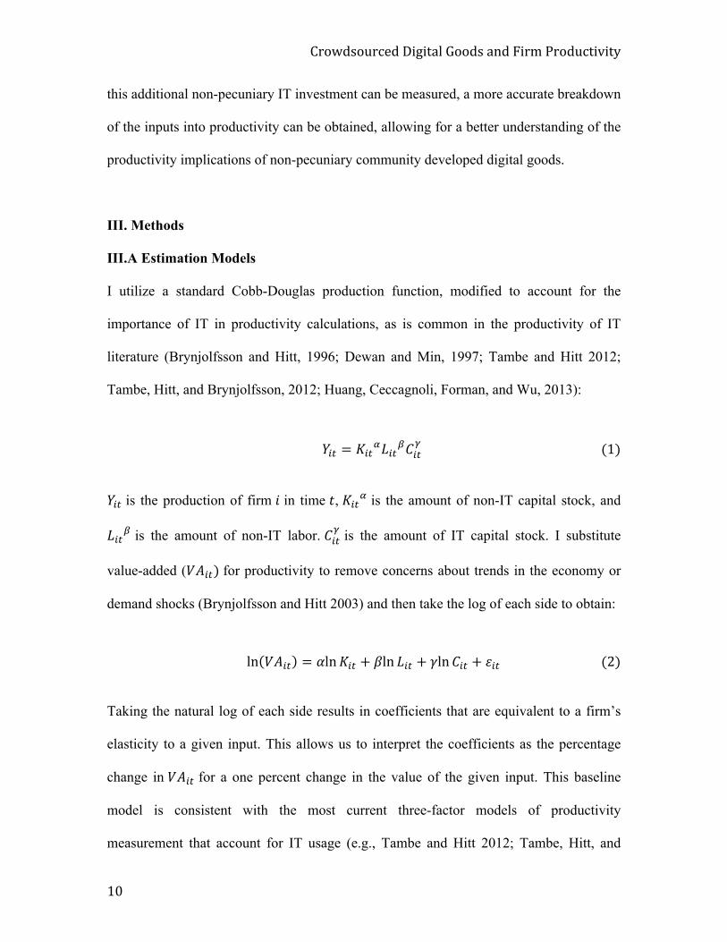
I utilize a standard Cobb-Douglas production function, modified to account for the

importance of IT in productivity calculations, as is common in the productivity of IT

literature (Brynjolfsson and Hitt, 1996; Dewan and Min, 1997; Tambe and Hitt 2012;

Tambe, Hitt, and Brynjolfsson, 2012; Huang, Ceccagnoli, Forman, and Wu, 2013):

!!" ! !!"!!!"

!!!"

!!!!!!!!!!!!!!!!!!!!!!!!!!!!!!!!!!!!!!!!!!!!!!!!!!!!!!!!!!!!!

!!" is the production of firm ! in time !, !!"! is the amount of non-IT capital stock, and

!!"! is the amount of non-IT labor. !

!"

! is the amount of IT capital stock. I substitute

value-added (!!!"! for productivity to remove concerns about trends in the economy or

demand shocks (Brynjolfsson and Hitt 2003) and then take the log of each side to obtain:

!" !!!" ! !!"!!" ! !!" !!" ! !!"!!" ! !!"!!!!!!!!!!!!!!!!!!!!!!!!!!!!!!!!!!!

Taking the natural log of each side results in coefficients that are equivalent to a firm’s

elasticity to a given input. This allows us to interpret the coefficients as the percentage

change in !!!" for a one percent change in the value of the given input. This baseline

model is consistent with the most current three-factor models of productivity

measurement that account for IT usage (e.g., Tambe and Hitt 2012; Tambe, Hitt, and

!"#$%&#'"()%*+,-,./0*1##%&*/2%*3,"4*5"#%'(.,6,.7*

99*

Brynjolfsson, 2012; Huang, Ceccagnoli, Forman, and Wu, 2013). However, notably

absent is the stock of free and open source software utilized by the firm. As discussed

above, because this software does not have a price, it is not accounted for in standard

productivity calculations. To account for this properly, I enhance this model with a

measure of a firm’s utilization of non-pecuniary open source software,

!"!!!"#$%&'()!!""!", in a given period. Non-pecuniary OSS must be separated from

pecuniary OSS because the latter is already measured by current productivity methods

since it has a price.5 I again take the natural log of this measure to allow for consistent

interpretation. This results in the following equation:

!" !!!" ! !!"!!" ! !!" !!" ! !!!"!!" ! !! !"!"!!!"#$%&'()!!""!" ! !!"!!!!!!!!!

To control for the firm’s investment in other operating system software, I also include a

measure of the total number of pecuniary OSS operating systems (!"#$%&'()!!""!"! as

well as closed source operating systems (!"#$%&!"! at the firm in a given period. These

two variables are also transformed by taking the natural log, yielding the following

equation:

!" !!!" ! !!"!!" ! !!" !!" ! !!!"!!" ! !! !"!"!!!"#$%&'()!!""!"

! !! !"!"#$%!"#$!!""!" ! !! !" !"#$%&!" ! !!"!!!!!!!!!!!!!!!!!!!!!!!!!!!!!!!!!!!!!!!!!!

********************************************************5 As mentioned above, an important aspect of the OSS movement is the ability to build pecuniary

software on top of non-pecuniary OSS. For example, Red Hat Enterprise Linux is built on the open source Linux kernel, but is not free due to the additional functionality and support Red Hat

provides. Similarly, Apple charges a pecuniary price for Mac OS X although it is built on the

open source FreeBSD kernel. Conversely, a product like Mandrake Linux is both open source and

non-pecuniary. Therefore, we must consider this pecuniary OSS differently than non-pecuniary OSS.

!"#$%&#'"()%*+,-,./0*1##%&*/2%*3,"4*5"#%'(.,6,.7*

98*

Using equation 4 as my preferred estimation equation, I will also estimate the impact of

OSS usage in a binary manner.

III.B Identification Strategy

Like all studies of the impact of IT on productivity, my analysis is subject to both errors

in the measurement of the variables, and endogeneity. The former could result in

attenuation bias, underestimating the size of the effect, while the latter could lead to an

overestimation of the effect if firms that use OSS tend to have higher levels of

productivity but the relationship is not causal. Therefore, I employ a number of methods

that help to address both of these concerns.

First, since I am using panel data, I will use firm random effect models to estimate the

effect at individual firms. Further, to control for unobserved time and industry trends, I

add a year fixed effect and industry fixed effect at the 1-digit Standard Industrial

Classification (SIC) level. The combination of these approaches helps eliminate

unobserved firm, time, or industry effects that may bias the results.

Second, I will employ an instrumental variable to help address both endogeneity and

errors-in-variables bias. My instrument is a measure of the mean non-pecuniary OSS

usage within a firm’s 2-digit SIC industry within the same year. These firms face supply

conditions similar to the focal firm. The amount of non-pecuniary OSS usage by the

firms in a firm’s same industry may affect that firm’s propensity for using non-pecuniary

OSS, but does not directly affect the firm’s productivity level. I will use this instrument

!"#$%&#'"()%*+,-,./0*1##%&*/2%*3,"4*5"#%'(.,6,.7*

9G*

within a framework that also employs random effects.

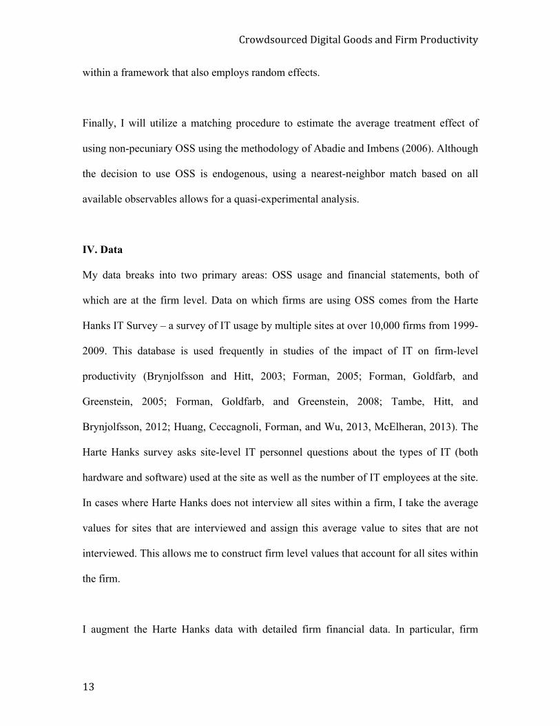
Finally, I will utilize a matching procedure to estimate the average treatment effect of

using non-pecuniary OSS using the methodology of Abadie and Imbens (2006). Although

the decision to use OSS is endogenous, using a nearest-neighbor match based on all

available observables allows for a quasi-experimental analysis.

IV. Data

My data breaks into two primary areas: OSS usage and financial statements, both of

which are at the firm level. Data on which firms are using OSS comes from the Harte

Hanks IT Survey – a survey of IT usage by multiple sites at over 10,000 firms from 1999-

2009. This database is used frequently in studies of the impact of IT on firm-level

productivity (Brynjolfsson and Hitt, 2003; Forman, 2005; Forman, Goldfarb, and

Greenstein, 2005; Forman, Goldfarb, and Greenstein, 2008; Tambe, Hitt, and

Brynjolfsson, 2012; Huang, Ceccagnoli, Forman, and Wu, 2013, McElheran, 2013). The

Harte Hanks survey asks site-level IT personnel questions about the types of IT (both

hardware and software) used at the site as well as the number of IT employees at the site.

In cases where Harte Hanks does not interview all sites within a firm, I take the average

values for sites that are interviewed and assign this average value to sites that are not

interviewed. This allows me to construct firm level values that account for all sites within

the firm.

I augment the Harte Hanks data with detailed firm financial data. In particular, firm

!"#$%&#'"()%*+,-,./0*1##%&*/2%*3,"4*5"#%'(.,6,.7*

9M*

expenditures on labor (IT and non-IT) and capital (IT and non-IT) as well as firm

revenues and costs of materials. For public firms, this information is available via

Standard and Poor’s Compustat database. To match the Harte Hanks data to the

Compustat data, I used the firm’s stock ticker symbol which is present in both datasets. In

this manner, sites within the Harte Hanks database that are owned by different firms in

different years (e.g., through mergers or acquisitions) will be associated with the correct

parent firm and therefore the correct financial data. The sections below detail how these

two datasets are used to construct the variables discussed in the previous section. For all

monetary values, I convert the value to 2009 dollars using an appropriate deflation index

and report the value in millions of dollars.

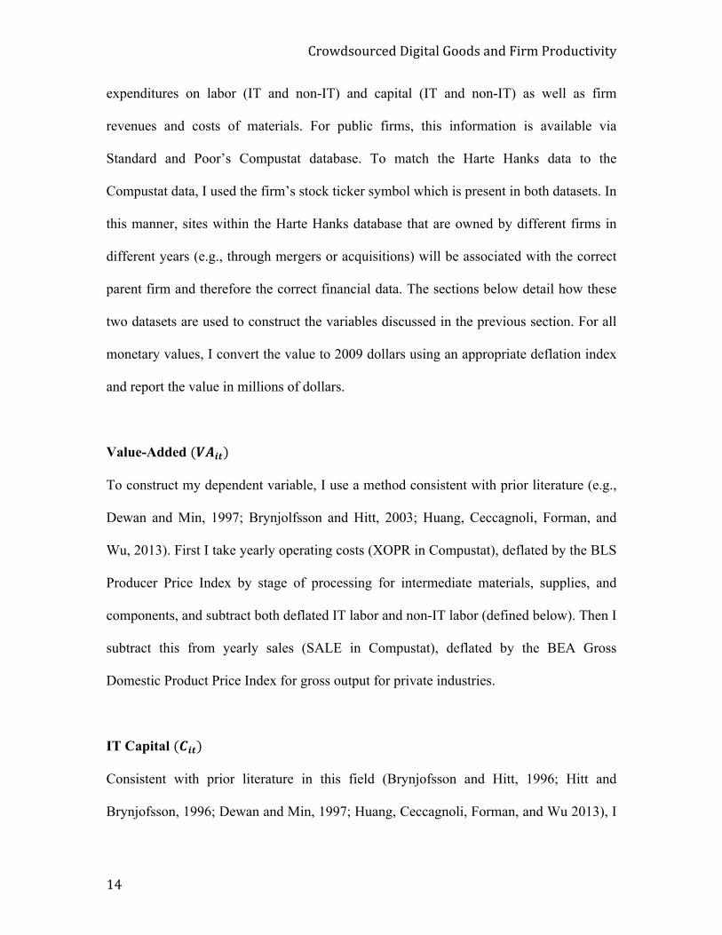
Value-Added !!!!"!

To construct my dependent variable, I use a method consistent with prior literature (e.g.,

Dewan and Min, 1997; Brynjolfsson and Hitt, 2003; Huang, Ceccagnoli, Forman, and

Wu, 2013). First I take yearly operating costs (XOPR in Compustat), deflated by the BLS

Producer Price Index by stage of processing for intermediate materials, supplies, and

components, and subtract both deflated IT labor and non-IT labor (defined below). Then I

subtract this from yearly sales (SALE in Compustat), deflated by the BEA Gross

Domestic Product Price Index for gross output for private industries.

IT Capital !!!"!

Consistent with prior literature in this field (Brynjofsson and Hitt, 1996; Hitt and

Brynjofsson, 1996; Dewan and Min, 1997; Huang, Ceccagnoli, Forman, and Wu 2013), I

!"#$%&#'"()%*+,-,./0*1##%&*/2%*3,"4*5"#%'(.,6,.7*

9N*

construct a measure that includes both the value of IT hardware at the firm and three

times the value of IT labor at the firm. This is a commonly used estimation of the full

value of IT capital due to the importance of IT labor being used for internal software

development efforts, the result of which is a capital good.

To do this, I first estimate the market value of the IT stock by multiplying the number of

PCs and Servers at the firm (from Harte Hanks6) by the average value of a PC or Server

that year from The Economist Intelligence Unit Telecommunications Database. I then

deflate this by the BEA Price Index for computers and peripherals.

I then calculate the value of IT labor by taking the number of IT workers at each firm

(from Harte Hanks 7) multiplied by the mean annual wage for all Computer and

Mathematical Science Occupations8. I deflate the result by the BLS Employment Cost

Index for wages and salaries for private industry workers. I multiply the result by three

and add the PC and Server value above to obtain the aggregate measure !!".

Non-IT Capital !!!"!

To construct the !!" variable, I take the yearly Gross Total Property, Plant and Equipment

********************************************************6 For most firms, Harte Hanks only surveys a sample of the sites within the firm. In such cases, I

calculate the average number of PCs and Servers at the sites that are in the survey, and then multiply by the total number of sites in the firm to obtain the total number of PCs and Servers in

the firm. I use the same procedure for calculating the number of IT employees and the number of

each type of operating system at the firm. 7 Harte Hanks reports the number of IT employees at each site as a range so I take the average

value of the range. The ranges are 1-4, 5-9, 10-24, 25-49, 50-99, 100-249, 250-499, and 500 or

More. 8 Obtained from the Bureau of Labor and Statistics:

http://www.bls.gov/oes/2009/may/oes_nat.htm#15-0000.

!"#$%&#'"()%*+,-,./0*1##%&*/2%*3,"4*5"#%'(.,6,.7*

9O*

(PPEGT in Compustat), deflated by the BLS price index for Detailed Capital Measures

for All Assets for the Private Non-Farm Business Sector, and subtract the deflated value

of IT Capital (defined above).

Non-IT Labor !!!"!

I take the total number of employees at the firm (EMP in Compustat) and subtract the

number of IT employees (from Harte Hanks) to obtain the total number of non-IT

employees. I then multiply this by the mean annual wage of all occupations9 that year. I

deflate the result by the BLS Employment Cost Index for wages and salaries for private

industry workers. This method of calculation is consistent with prior studies on IT

productivity (Bloom and Van Reenen, 2007; Bresnahan, Brynjolfsson, and Hitt, 2002;

Brynjolfsson and Hitt 2003).

Operating Systems Measures

I construct these three measures ( !"!!!"#$%&'()!!""!" !!"#$%&'()!!""!" ! and

!"#$%&!") by calculating the total number of each type of operating system at the firm

(from Harte Hanks). The Harte Hanks data does not report the precise number of

operating systems in use at a given firm. It does, however, report the different types of

operating systems used at each site. I classify these operating systems into three

categories, non-pecuniary OSS, pecuniary OSS, or closed source. Further, Harte Hanks

reports whether each operating system is for a PC or a server as well as the total number

of PCs and servers at each site. Therefore, for each site, I assume an even split of the

********************************************************9 Obtained from the Bureau of Labor and Statistics, for example the data for 2009 can be found

here: http://www.bls.gov/oes/2009/may/oes_nat.htm#00-0000.

!"#$%&#'"()%*+,-,./0*1##%&*/2%*3,"4*5"#%'(.,6,.7*

9P*

number of PC operating systems over the total number of PCs at the site. I do the same

for servers. This yields an estimate of how many instances of a given type of operating

system exist at the site. I then aggregate this to the firm level and divide by the number of

sites at the firm in the Harte Hanks database to obtain an average per site. Finally, I

multiply this by the total number of sites in the firm to obtain a firm-wide estimate of the

number of each type of operating system. As the resulting numbers are estimates, I will

begin my analysis by only using a binary indicator of the presence of each type of

operating system. The estimated number of operating systems will then allow for a more

granular interpretation of the primary effect.

Because the number of operating systems in any of the three categories can potentially be

zero (e.g., that category of operating system is not in use at the firm), I add one to the

number of operating systems in each category before taking the natural log as the natural

log of zero is undefined. Although there are many firms that have zero non-pecuniary and

pecuniary OSS operating systems, there is a high degree of skewness in these numbers

(as shown in the descriptive statistics below). Therefore, adding a one before taking the

natural log should not significantly bias the results.

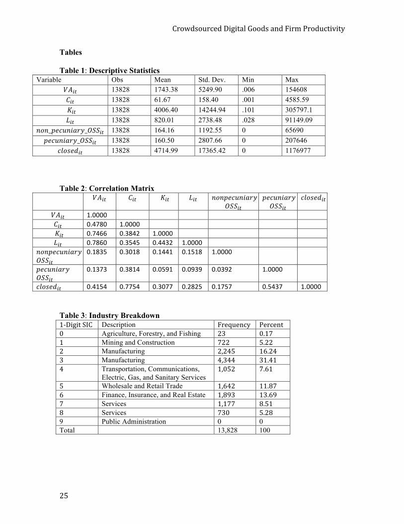
Table 1 shows the descriptive statistics of the firms in my dataset. There are 13,828

firm/year observations in the dataset. The ranges vary greatly for all variables and

demonstrate the breadth of the firms in the sample. This breadth allows for results that are

more generalizable than many other studies of this kind, which only focus on Fortune

1000 companies. The firms in the dataset also have a wide range of the type and intensity

!"#$%&#'"()%*+,-,./0*1##%&*/2%*3,"4*5"#%'(.,6,.7*

9Q*

of IT use. The mean number of closed source operating systems at a firm is 4714.99

while the mean number of non-pecuniary OSS and pecuniary OSS operating systems are

much lower at 164.16 and 160.50, respectively. Table 2 shows the correlation matrix and

Table 3 shows the breakdown by industry.

-------------------

Insert Tables 1, 2, & 3 Here -------------------

V. Results

Three-Factor Productivity Analysis

Before delving into the results on open source usage, I first present the results of the

baseline regression, equation 2, to compare the elasticities of the three main productivity

inputs with other existing studies. Table 4 shows the results of my basic three-factor

productivity analysis. Models 1-3 use Ordinary Least Squares (OLS) regression with

increasingly restrictive fixed effects, while Model 4 uses panel regression with firm fixed

effects and Model 5 uses panel regression with random effects. For all models, the

standard errors are robust and clustered by firm. The high R2 values are characteristic of

such productivity studies. The confidence intervals of the coefficients in models 4 and 5

overlap with those of Huang, Ceccagnoli, Forman, and Wu (2013), whose methodology

this study most closely resembles. However, my coefficients on non-IT capital are

slightly higher than theirs, likely because their sample size is only companies in the

Fortune 1000, while I cast a wider net. However, as a robustness check I will later split

the sample and analyze Fortune 1000 firms separately to confirm this is not skewing my

results. Further, the model 4 coefficient on IT capital is very similar to that of

!"#$%&#'"()%*+,-,./0*1##%&*/2%*3,"4*5"#%'(.,6,.7*

9R*

Brynjolfsson and Hitt (2003) in their 1-year difference model with year and industry

controls. The coefficients for model 4 are also very similar to the fixed effect estimate of

Tambe and Hitt (2012), although the IT capital coefficient is slightly lower, likely

because they are calculating their coefficient based solely on IT labor. These similarities

help to add support to the validity of my dataset.

-------------------

Insert Table 4 Here -------------------

Binary Usage of Non-Pecuniary OSS

Table 5 presents my estimation results using a binary measure of OSS usage. Columns 1,

2, and 5 show the results of estimating equation 3, which does not include the controls for

other types of operating systems. Columns 3, 4, and 6 show the result of estimating

equation 4, which includes these controls. Although columns 1-4 show a slight positive

coefficient for !"#$%&!!"!!!"#$%&'()!!""!", the coefficients are not significant. As the

rest of my analysis shows, in all models using instrumental variables, this coefficient is

significant, implying there may be an attenuation bias resulting in an underestimate of

these coefficients in the basic panel models. Columns 5 and 6 show the results from the

random effect estimation with the same industry non-pecuniary OSS instrument. Both

models show a positive and significant coefficient for !"#$%&!!"!!!"#$%&'()!!""!".

Additionally, both models have a first stage F-statistic much greater than 10, adding

validity to the relevance of my instrument. The coefficients in these two models are

nearly identical, indicating that the !"#$%&!!"!!!"#$%&'()!!""!" variable is not just

identifying firms who invest in more IT (operating systems), but that the effect is due to

!"#$%&#'"()%*+,-,./0*1##%&*/2%*3,"4*5"#%'(.,6,.7*

8<*

the adoption of non-pecuniary OSS. Since the dependent variable is a natural log, we can

interpret the coefficient on !"#$%&!!"!!!"#$%&'()!!""!" to indicate that firms who use

non-pecuniary OSS have a 1.03% increase in productivity (as measured by value-added).

-------------------

Insert Table 5 Here -------------------

Continuous Usage of Non-Pecuniary OSS

Table 6 presents my estimation results using a continuous measure of OSS usage. As in

Table 5, columns 1, 2, and 5 show the results of estimating equation 3, which does not

include the controls for other types of operating systems and columns 3, 4, and 6 show

the result of estimating equation 4, which includes these controls. Again, columns 1-4

show a slight positive coefficient for the continuous measure of !"!!!"#$%&'()!!""!",

but the coefficients are not significant. However, columns 5 and 6 show the results from

the random effect estimation with the same industry non-pecuniary OSS instrument,

which shows a positive and significant coefficient for !"!!!"#$%&'()!!""!". Again,

both models have a first stage F-statistic much greater than 10, adding validity to the

relevance of my instrument. As with the binary analysis, the coefficients in these two

models are nearly identical, indicating that the !"!!!"#$%&'()!!""!" variable is not just

identifying firms who invest in more IT (operating systems), but that the effect is due to

the usage of non-pecuniary OSS. Since the estimation is a log-log specification, we can

interpret the coefficient on !"!!!"#$%&'()!!""!" to mean that a 1% increase in the

amount of non-pecuniary OSS a firm uses leads to a .15% increase in productivity (as

measured by value-added). By comparison, this represents a little more than half the

!"#$%&#'"()%*+,-,./0*1##%&*/2%*3,"4*5"#%'(.,6,.7*

89*

elasticity for non-IT capital. The reduction of the coefficient on IT Capital to the point

where it is either not significant or negative is symptomatic of such studies (Huang,

Ceccagnoli, Forman, and Wu, 2013).

-------------------

Insert Table 6 Here -------------------

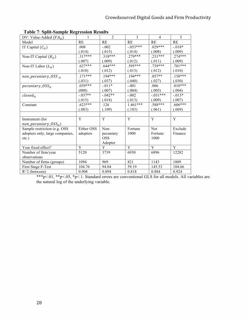
Split-Sample Analysis

To further explore the results, I use my preferred specification (model 6 from Table 6) to

calculate various split-sample results. Table 7 shows the results of this analysis. In

column 1, I examine the continuous effect on only firms who are users of either non-

pecuniary or pecuniary OSS. In column 2, I look at only firms that use non-pecuniary

OSS. In both cases, the coefficient on !"!!!"#$%&'()!!""!!" is higher than in the full

sample, however the confidence intervals all overlap.

Column 3 only uses firms that were in the Fortune 1000 at least one year from 1999-

2009. The coefficient on !"!!!"#$%&'()!!""!"!is slightly larger, but statistically not

different than that when using the full sample. This allows me to further confirm that my

results are consistent with prior literature (Brynjolfsson and Hitt, 2003; Tambe and Hitt,

2012;*Huang, Ceccagnoli, Forman, and Wu, 2013), and are not driven by differences in

the makeup of my sample. However, the results in column 4 show a slightly different

story for firms that are not in the Fortune 1000. These firms are generally smaller than the

Fortune 1000 firms, and we see that these smaller firms obtain a benefit to using non-

!"#$%&#'"()%*+,-,./0*1##%&*/2%*3,"4*5"#%'(.,6,.7*

88*

pecuniary OSS that is statistically lower. Finally, in column 5, I exclude finance

companies from my sample because they frequently report capital expenditures in a

fundamentally different way than other firms. The resulting coefficient for

!"!!!!"#$%&'(!!""!" is nearly identical to that in the full sample, indicating that this

irregularity does not affect my results.*

-------------------

Insert Table 7 Here -------------------

Average Treatment Effect of Non-Pecuniary OSS Usage

Finally, I also utilized a matching procedure to estimate the average treatment effect of

using OSS by employing the methodology of Abadie and Imbens (2006). While the

decision to use OSS is not exogenous, matching allows for quasi-experimental analysis.

Using a nearest-neighbor match based on all observables used in the prior regressions, I

construct a matched sample based on the binary use of non-pecuniary OSS. I then use this

matched sample to estimate the sample average treatment effect (SATE) at .181 with a

standard error of .031. This positive and statistically significant coefficient again offers

support for the validity of my primary results.

VI. Discussion and Conclusion

My results show that the consumption of non-pecuniary OSS does indeed have an impact

on the productivity of the firm, and that this impact is positive. Although this result did

not appear significant in the basic panel regression, it is consistently significant in all

specifications that account for endogeneity and errors-in-variables via instrumental

!"#$%&#'"()%*+,-,./0*1##%&*/2%*3,"4*5"#%'(.,6,.7*

8G*

variable analysis and a quasi-experimental approach via the Abadie and Imbens nearest-

neighbor match. The effect stays consistent in sub-sample analyses of OSS adopters,

Fortune 1000 firms, and non-finance firms. I also show that this effect exists when

considering the use of non-pecuniary OSS at a binary level.

Interestingly, a slight negative return to the usage of closed source software appeared in

several of the estimation models. However, this effect was not consistent throughout the

more rigorous models. Likewise, the effect of pecuniary OSS was not stable throughout

the various analyses. As these two variables were only used as controls, it is difficult to

make a general statement about their specific effect on productivity.

Although endogeneity is always a concern in productivity studies, I take many steps to

help rule out this bias and allow for a causal statement. All of the primary regression

results (Tables 5 and 6) use panel regression techniques with random effects as well as

fixed effects for year. This helps to rule out alternative explanations due to trends over

time so that I am comparing a firm with itself over time. The use of an instrumental

variable allows for a proper identification of the effect within this panel framework.

Further, the results of the various estimations of equation 4, which includes the number of

pecuniary OSS and closed source operating systems, allow us to rule out the concern that

a firm’s level of technology usage causes them to adopt non-pecuniary OSS and to have a

higher value-add, rather than the use of the non-pecuniary OSS itself causing the increase

in value-add. Finally, I use Abadie and Imbens’ nearest-neighbor match, to further reduce

concerns about endogeneity. With this statistically rigorous matching method, the

!"#$%&#'"()%*+,-,./0*1##%&*/2%*3,"4*5"#%'(.,6,.7*

8M*

primary finding of a positive causal effect of non-pecuniary OSS usage on productivity

holds.

My findings have important implications for researchers, practitioners, and policy

makers. For researchers, my results draw additional attention to the mismeasurement that

occurs when firms use OSS (and, more generally, non-pecuniary crowdsourced digital

goods) as inputs into production. Future studies of productivity, especially the

productivity of IT, should account for these non-pecuniary inputs, rather than lumping

them into firm intangible effects. This is especially important as information costs are

approaching zero and the amount of non-pecuniary digital inputs firms use is likely to

rise in the coming years. For practitioners, my results indicate that firms of all sizes may

enhance their productivity by increasing the amount of OSS they employ in their

production process. For policy makers, my results indicate that federal funding of OSS

and other publicly available digital goods could enhance the productivity of firms. While

other studies have shown that federal investment in such goods can have a high rate of

return based on the value of the goods themselves, my results indicate that such goods

can also boost the productivity of the firms that use them.

!"#$%&#'"()%*+,-,./0*1##%&*/2%*3,"4*5"#%'(.,6,.7*

8N*

Tables

Table 1: Descriptive Statistics

Variable Obs Mean Std. Dev. Min Max

!!!" 13828 1743.38 5249.90 .006 154608

!!" 13828 61.67 158.40 .001 4585.59

!!!" 13828 4006.40 14244.94 .101 305797.1

!!" 13828 820.01 2738.48 .028 91149.09

!"!!!!"#$%&'(!!""!" 13828 164.16 1192.55 0 65690

!"#$%&'()!!""!" 13828 160.50 2807.66 0 207646

!"#$%&!" 13828 4714.99 17365.42 0 1176977

Table 2: Correlation Matrix

!!!" !!" !!!" !!" !!"#$%&"'()*

!"!!"

!"#$%&'()

!"!!"

!"#$%&!"

!!!" !"####

!!" #"$%&# !"####

!!!" #"%$'' #"(&$) !"####

!!" #"%&'# #"(*$* #"$$() !"####

!"!#$%&!'()*

!"!!"

#"!&(* #"(#!& #"!$$! #"!*!& !"####

!"#$%&'()

!"!!"

#"!(%( #"(&!$ #"#*+! #"#+(+ #"#(+) !"####

!"#$%&!" #"$!*$ #"%%*$ #"(#%% #")&)* #"!%*% #"*$(% !"####

!

!

Table 3: Industry Breakdown

9K+,-,.*:D! Description 3")S')2(7 5)"()2.

< Agriculture, Forestry, and Fishing 8G <?9P

9 Mining and Construction P88 N?88

8 Manufacturing 8;8MN 9O?8M

G Manufacturing M;GMM G9?M9

M Transportation, Communications,

Electric, Gas, and Sanitary Services 9;<N8 P?O9

N Wholesale and Retail Trade 9;OM8 99?QP

O Finance, Insurance, and Real Estate 9;QRG 9G?OR

P Services 9;9PP Q?N9

Q Services PG< N?8Q

9 Public Administration 0 0

Total 13,828 100

!"#$%&#'"()%*+,-,./0*1##%&*/2%*3,"4*5"#%'(.,6,.7*

8O*

Table 4: Baseline Regression Results DV: Value-Added !!!!"! 1 2 3 4 5

Model OLS OLS OLS FE RE

IT Capital !!!"! .072***

(.006)

.040***

(.006)

.032***

(.006)

.015***

(.005)

.019***

(.005)

Non-IT Capital !!!"! .320***

(.012)

.317***

(.012)

.304***

(.012)

.108***

(.034)

.269***

(.013)

Non-IT Labor !!!"!

.646***

(.014)

.665***

(.014)

.684***

(.015)

.758***

(.032)

.716***

(.016)

Constant .278***

(.040)

.091**

(.045)

.127

(.160)

.980***

(.162)

.219**

(.086)

Year fixed effect? N Y Y Y Y

Industry fixed effect (SIC2) N N Y Y Y

Number of firm/year observations 13828 13828 13828 13828 13828

Number of firms (groups) 1964 1964 1964 1964 1964

R^2 (between for panel) 0.897 0.911 0.915 0.912 0.930

***p<.01, **p<.05, *p<.1. All standard errors are clustered at the firm level. All variables are the natural log of the underlying variable.

!

Table 5: Binary OSS Regression Results DV: Value-Added !!!!"! 1 2 3 4 5 6

Model RE RE RE RE RE RE

IT Capital !!!"! .019***

(.005)

.018***

(.005)

.025***

(.005)

.024***

(.005)

-.028**

(.011)

-.026**

(.011)

Non-IT Capital !!!"! .276***

(.013)

.269***

(.013)

.278***

(.013)

.270***

(.013)

.288***

(.008)

.291***

(.007)

Non-IT Labor !!!"!

.707***

(.016)

.716***

(.016)

.710***

(.016)

.718***

(.016)

.677***

(.008)

.678***

(.009)

!"#$%&

!"!!!"#$%&'(!!!""!!"

.006

(.013)

.008

(.013)

.005

(.013)

.007

(.013)

1.036***

(.201)

1.034***

(.197)

!"#$%&'()!!""!" -.003

(.003)

-.003

(.003)

-.002

(.003)

!"#$%&!" -.012* (.007)

-.012* (.008)

-.006 (.008)

Constant .167***

(.051)

.220***

(.086)

.220***

(.057)

.273***

(.088)

.618***

(.065)

.638***

(.074)

Year fixed effect? Y Y Y Y Y Y

Industry fixed effect? N Y N Y N N

Instrument (for

!"!!!"#$%&'()!!""!")

N/A N/A N/A N/A Y Y

Number of firm/year

observations

13828 13828 13828 13828 13828 13828

Number of firms (groups) 1964 1964 1964 1964 1964 1964

First Stage F-test - - - - 70.91 74.62

R^2 (between) 0.926 0.930 0.926 0.930 0.908 0.908

***p<.01, **p<.05, *p<.1. Standard errors are clustered at the firm level for models 1-4, and

conventional GLS for models 5-6. All variables are the natural log of the underlying variable.

! !

!"#$%&#'"()%*+,-,./0*1##%&*/2%*3,"4*5"#%'(.,6,.7*

8P*

Table 6: Continuous OSS Regression Results DV: Value-Added !!!!"! 1 2 3 4 5 6

Model RE RE RE RE RE RE

IT Capital !!!"! .020*** (.005)

.018*** (.005)

.025*** (.005)

.024*** (.006)

-.016* (.008)

-.015 (.009)

Non-IT Capital !!!"! .276***

(.013)

.269***

(.013)

.277***

(.013)

.270***

(.013)

.276***

(.008)

.279***

(.008)

Non-IT Labor !!!"!

.707***

(.016)

.716***

(.016)

.710***

(.016)

.718***

(.016)

.687***

(.009)

.686***

(.009)

!"!!!"#$%&'()!!""!!" .001

(.003)

.001

(.003)

.0003

(.003)

.001

(.003)

.150***

(.029)

.155***

(.030)

!"#$%&'()!!""!" -.003

(.003)

-.003

(.003)

.008*

(.004)

!"#$%&!" -.012*

(.007)

-.012*

(.007)

-.006

(.007)

Constant .167***

(.051)

.221***

(.086)

1.220***

(.057)

.274***

(.088)

.618***

(.061)

.641***

(.067)

Year fixed effect? Y Y Y Y Y Y

Industry fixed effect? N Y N Y N N

Instrument (for

!"!!!"#$%&'()!!""!")

N/A N/A N/A N/A Y Y

Number of firm/year

observations

13828 13828 13828 13828 13828 13828

Number of firms (groups) 1964 1964 1964 1964 1964 1964

First Stage F-test - - - - 112.00 107.58

R^2 (between) 0.926 0.930 0.926 0.930 0.918 0.917

***p<.01, **p<.05, *p<.1. Standard errors are clustered at the firm level for models 1-4, and

conventional GLS for models 5-6. All variables are the natural log of the underlying variable.

*

* *

!"#$%&#'"()%*+,-,./0*1##%&*/2%*3,"4*5"#%'(.,6,.7*

8Q*

Table 7: Split-Sample Regression Results DV: Value-Added !!!!"! 1 2 3 4 5

Model RE RE RE RE RE

IT Capital !!!"! .008 (.014)

-.002 (.015)

-.053*** (.014)

.029*** (.008)

-.018* (.009)

Non-IT Capital !!!"! .317***

(.007)

.318***

(.009)

.279***

(.012)

.231***

(.011)

.274***

(.009)

Non-IT Labor !!!"!

.627***

(.010)

.644***

(.012)

.595***

(.013)

.739***

(.012)

.701***

(.010)

!"!!!"#$%&'()!!""!!" .171***

(.031)

.194***

(.037)

.194***

(.040)

.057**

(.027)

.158***

(.030)

!"#$!"#$%!!""!" .039***

(008)

-.011*

(.007)

-.001

(.004)

.006

(.005)

.010***

(.004)

!"#$%&!" -.037**

(.015)

-.042**

(.018)

-.002

(.013)

-.031***

(.009)

-.013*

(.007)

Constant .623***

(.083)

.126

(.109)

1.461***

(.183)

.588***

(.061)

.606***

(.069)

Instrument (for

!"!!!"#$%&'()!!""!")

Y Y Y Y Y

Sample restriction (e.g. OSS

adopters only, large companies,

etc.)

Either OSS

adopters

Non-

pecuniary

OSS

Adopter

Fortune

1000

Not

Fortune

1000

Exclude

Finance

Year fixed effect? Y Y Y Y Y

Number of firm/year

observations

5120 3739 6930 6896 12282

Number of firms (groups) 1094 969 821 1143 1809

First Stage F-Test 104.76 94.04 59.19 145.53 104.66

R^2 (between) 0.908 0.894 0.818 0.884 0.924

***p<.01, **p<.05, *p<.1. Standard errors are conventional GLS for all models. All variables are the natural log of the underlying variable.

!"#$%&#'"()%*+,-,./0*1##%&*/2%*3,"4*5"#%'(.,6,.7*

8R*

References

Abadie, A., & Imbens, G. W. (2006). Large sample properties of matching estimators for average

treatment effects. Econometrica, 74(1), 235-267. Altman, E., Nagle, F., & Tushman, M. (2014). Innovating without Information Constraints:

Organizations, Communities, and Innovation When Information Costs Approach Zero.

Harvard Business School Working Paper.

Aral, S., & Weill, P. (2007). IT assets, organizational capabilities, and firm performance: How resource allocations and organizational differences explain performance variation.

Organization Science, 18(5), 763-780.

Baldwin, C., & Von Hippel, E. (2011). Modeling a Paradigm Shift: From Producer Innovation to User and Open Collaborative Innovation. Organization Science, 22(6), 1399–1417.

Bloom, N. & J. Van Reenen. (2007). Measuring and explaining management practices across

firms and countries. Quarterly Journal of Economics. 122(4) 1351-1408. Bresnahan, T.F., E. Brynjolfsson, & L.M. Hitt. (2002). Information technology, workplace

organization, and the demand for skilled labor: Firm-level evidence. Quarterly Journal of

Economics. 117(1) 339-376.

Bridgman, B. (2013). Home Productivity. Bureau of Economic Analysis Working Paper 2013-03. Brynjolfsson, E., & Hitt, L. (1996). Paradox lost? Firm-level evidence on the returns to

information systems spending. Management science, 42(4), 541-558.

Brynjolfsson, E., & Hitt, L. M. (2003). Computing productivity: Firm-level evidence. Review of

economics and statistics, 85(4), 793-808.

Brynjolfsson, E., Hitt, L. M., & Yang, S. (2002). Intangible assets: Computers and organizational

capital. Brookings papers on economic activity, 2002(1), 137-198. Byrne, D., Oliner, S., & Sichel, D. (2013). Is the information technology revolution over?

Available at SSRN 2240961.

Casadesus-Masanell, R., & Llanes, G. (2011). Mixed Source. Management Science, 57(7), 1212–

1230. Dewan, S., & Min, C. K. (1997). The substitution of information technology for other factors of

production: A firm level analysis. Management Science, 43(12), 1660-1675.

Forman, C. (2005). The corporate digital divide: Determinants of Internet adoption. Management

Science, 51(4), 641-654.

Forman, C., Goldfarb, A., & Greenstein, S. (2005). How did location affect adoption of the

commercial Internet? Global village vs. urban leadership. Journal of Urban Economics, 58(3),

389-420. Forman, C., Goldfarb, A., & Greenstein, S. (2008). Understanding the inputs into innovation: Do

cities substitute for internal firm resources?. Journal of Economics & Management Strategy,

17(2), 295-316. Fitzgerald, B. (2006). The transformation of open source software. Mis Quarterly, 587-598.

Greenstein, S., & Nagle, F. (2014). Digital Dark Matter and the Economic Contribution of

Apache. National Bureau of Economic Research Working Paper 19507. Forthcoming in Research Policy.

Harhoff, D., Henkel, J., & Von Hippel, E. (2003). Profiting from voluntary information

spillovers: how users benefit by freely revealing their innovations. Research Policy, 32(10),

1753-1769. Hitt, L. M., & Brynjolfsson, E. (1996). Productivity, business profitability, and consumer surplus:

three different measures of information technology value. MIS Quarterly, 121-142.

Howe, J. 2008. Crowdsourcing: Why the Power of the Crowd is Driving the Future of Business.

Crown Business, New York.

Henkel, J. (2006). Selective revealing in open innovation processes: The case of embedded

Linux. Research policy, 35(7), 953-969.

!"#$%&#'"()%*+,-,./0*1##%&*/2%*3,"4*5"#%'(.,6,.7*

G<*

Huang, P., Ceccagnoli, M., Forman, C., & Wu, D. J. (2013). IT Knowledge Spillovers and

Productivity: Evidence from Enterprise Software. Available at SSRN 2243886. Jorgenson, D. W. (2001). Information technology and the US economy. The American Economic

Review, 91(1), 1-32.

Jorgenson, D. W., Ho, M. S., & Stiroh, K. J. (2005). Productivity, Volume 3: Information

Technology and the American Growth Resurgence. MIT Press Books, 3. Krishnamurthy, S. (2005). "An Analysis of Open Source Business Models," in Perspectives on

Free and Open Source Software, J. Feller, B. Fitzgerald, S. Hissam, and K. Lakhani (eds.),

MIT Press, Cambridge, MA, 2005, pp. 279-296. Lakhani, K., & Von Hippel, E. (2003). How open source software works: “free” user-to-user

assistance. Research Policy, 32(6), 923–943.

Lakhani, K., Lifshitz-Assaf, H., & Tushman, M. (2012). Open innovation and organizational boundaries: the impact of task decomposition and knowledge distribution on the locus of

innovation in Handbook of Economic Organization: Integrating Economic and Organization

Theory, A. Grandori (ed.), Edward Elgar Publishing, Northampton, MA, pp. 355-382.

Lerner, J., & Schaknerman, M. (2010). The comingled code: Open source and economic development. MIT Press Books, 1.

Lerner, J., & Tirole, J. (2002). Some Simple Economics of Open Source. The Journal of

Industrial Economics, 50(2), 197–234. MacCormack, A. (2003). Evaluating Total Cost of Ownership for Software Platforms: Comparing

Apples, Oranges, and Cucumbers. AEI-Brookings Joint Center for Regulatory Studies Related

Publication, April 2003. McElheran, K. S. (2013). Delegation in Multi-Establishment Firms: Adaptation vs. Coordination

in I.T. Purchasing Authority. Journal of Economics & Management Strategy, forthcoming.

O’Mahony, S. (2003). Guarding the commons: how community managed software projects

protect their work. Research Policy, 32(7), 1179–1198. Raymond, Eric. (1998). Goodbye, “free software”; hello, “open source”. Retrieved from

http://www.catb.org/~esr/open-source.html on February 23, 2014.

Russo, B., Braghin, B., Gasperi, P., Sillitti, A., and Succi, G. (2005). Defining TCO for the Transition to Open Source Systems. Proceedings of the First International Conference on

Open Source (OSS2005), pp. 108-112.

Schumpeter, Joseph. 1942. “The Process of Creative Destruction.” Chapter VII, pp. 81-86 in

Capitalism, Socialism, and Democracy. New York, NY: Harper & Row. Shirky, C. Here Comes Everybody: The Power of Organizing Without Organizations. Penguin

Press, New York.

Syverson, C. (2011). What Determines Productivity? Journal of Economic Literature, 49(2), pp. 326-365.

Tambe, P., & Hitt, L. M. (2012). The Productivity of Information Technology Investments!: New

Evidence from IT Labor Data. Information Systems Research, 23(3), 599–617. Tambe, P., Hitt, L., & Brynjolfsson, E. (2011). The Price and Quantity of IT-Related Intangible

Capital. Working paper.

Tambe, P., Hitt, L. M., & Brynjolfsson, E. (2012). The Extroverted Firm: How External

Information Practices Affect Innovation and Productivity. Management Science, 58(5), 843–859.

Von Hippel, E. (1986). Lead Users: A Source of Novel Product Concepts. Management Science,

32(7), 791–805. Von Hippel, E., & Von Krogh, G. (2003). Open source software and the “private-collective”

innovation model: Issues for organization science. Organization science, 14(2), 209-223.

Von Krogh, G., Spaeth, S., & Lakhani, K. R. (2003). Community, joining, and specialization in open source software innovation: a case study. Research Policy, 32(7), 1217–1241.

!"#$%&#'"()%*+,-,./0*1##%&*/2%*3,"4*5"#%'(.,6,.7*

G9*

West, J., & Lakhani, K. R. (2008). Getting clear about communities in open innovation. Industry

and Innovation, 15(2), 223-231. Wheeler, D. (2005). Why Open Source Software/Free Software (OSS/FS, FLOSS, or FOSS)?

Look at the Numbers! available online at http://www.dwheeler.com/oss_fs_why.html.

!

!