WP/15/264

Crowding-Out or Crowding-In? Public and Private Investment in India

by Girish Bahal, Mehdi Raissi, and Volodymyr Tulin

© 2015 International Monetary Fund WP/15/264

IMF Working Paper

Asia and Pacific Department

Crowding-Out or Crowding-In? Public and Private Investment in India 1

Prepared by Girish Bahal,2 Mehdi Raissi, and Volodymyr Tulin

Authorized for distribution by Paul Cashin

December 2015

Abstract

This paper contributes to the debate on the relationship between public-capital accumulation and

private investment in India along the following dimensions. First, acknowledging major structural

changes that the Indian economy has undergone in the past three decades, we study whether public

investment in recent years has become more or less complementary to private investment in

comparison to the period before 1980. Second, we construct a novel data-set of quarterly aggregate

public and private investment in India over the period 1996Q2-2015Q1 using investment-project data

from the CapEx-CMIE database. Third, embedding a theory-driven long-run relationship on the

model, we estimate a range of Structural Vector Error Correction Models (SVECMs) to re-examine

the public and private investment relationship in India. Identification is achieved by decomposing

shocks into those with transitory and permanent effects. Our results suggest that while public-capital

accumulation crowds out private investment in India over 1950-2012, the opposite is true when we

restrict the sample post 1980 or conduct a quarterly analysis since 1996Q2. This change can most

likely be attributed to the policy reforms which started during early 1980s and gained momentum

after the 1991 crises.

JEL Classification Numbers: C30; C32; E22; H54.

Keywords: India; Public investment; Private investment; Crowding in; Crowding out; Permanent

shocks; Structural identification; Vector error correction models.

Authors’ E-Mail Addresses: girish.bahal@gmail.com; mraissi@imf.org; vtulin@imf.org

1 We are grateful to Paul Cashin, Giancarlo Corsetti, Kalpana Kochhar, Siddharth Kothari, Aart Kraay, Pritha Mitra,

Rakesh Mohan, Sam Ouliaris, Markus Rodlauer, and Luis Serven for their comments and suggestions. 2 Faculty of Economics, University of Cambridge, UK.

IMF Working Papers describe research in progress by the author(s) and are published to

elicit comments and to encourage debate. The views expressed in IMF Working Papers are

those of the author(s) and do not necessarily represent the views of the IMF, its Executive Board,

or IMF management.

2

Contents Page

I. Introduction ......................................................................................................................... 3

II. Structural VECM ................................................................................................................. 5

III. Data ..................................................................................................................................... 8

IV. Empirical findings .............................................................................................................. 9

A. Quarterly analysis using post-liberalization data ....................................................... 12

V. Concluding remarks ........................................................................................................... 13

Appendix A ............................................................................................................................. 14

Appendix B ............................................................................................................................. 15

References ............................................................................................................................... 16

Figures

1. Structural Impulse Responses to Productivity and Public Investment Shocks (Annual) .. 22

2. Structural Impulse Responses to Productivity and Public Investment Shocks (Quarterly)23

Tables

1. Unit Root Tests ................................................................................................................ 19

2. Lag Orders and Cointegrating Rank of the VECMs ........................................................ 20

3. Loading Coefficients and Cointegrating Vectors ............................................................ 20

4. Short and Long Run Matrices .......................................................................................... 21

3

I. INTRODUCTION

The relationship between public-capital accumulation and private investment has received

renewed interest among academics and policy makers alike in the aftermath of the global

financial crisis. On the one hand, higher public investment may "crowd out" private

expenditure on capital goods, irrespective of the financing mechanism (including through

levying taxes or issuing debt). On the other hand, higher government spending on

infrastructure facilities (like roads, highways, and power) and/or health and education may

have a complementary impact on private sector investment by raising the marginal

productivity of private capital. The literature, which mostly relies on time-series and

cross-country regression analysis, finds mixed predictions on the relationship between private

investment and public-capital accumulation. We re-examine this relationship in India by

estimating a Structural Vector Error Correction Model (SVECM) in three variables (public

investment, private investment, and output) over the period 1950-2012.

We also investigate whether this relationship has changed over time after the policy reforms

that started during 1980s (using annual observations) as well as post liberalization in early

1990s (using quarterly data over the period 1996Q2-2015Q1 from the CapEx-CMIE

database), and compute the corresponding rupee response of private investment to an

equivalent increase in public investment. Our main contribution to the literature, on

public-private investment relation in emerging market economies, is our novel identification

strategy and the use of theory-driven long-run relationships in the analysis. While we solve

the identification problem by imposing restrictions on the long-run impact of the shocks, we

motivate those restrictions from an economic theory perspective, namely, the "great ratio" of

investment to output. We estimate a SVECM and decompose the structural shocks into those

with permanent and transitory effects on the level of the variables for identification. We find

that while public-capital accumulation crowds out private investment in India over the full

sample 1950-2012, the opposite is true when we restrict the sample post 1980 or employ a

quarterly model of public-private investment since 1996Q2, largely due to policy reforms

introduced since the early 1990s.

We rely on long-run restrictions for identification, as they are typically free of particular

model assumptions and are motivated from what is generally agreed-upon in empirical

macroeconomic modeling, see Chudik et al. (2015a, 2015b) for details. This is in contrast to

solving the identification problem in VAR models by imposing short-run restrictions, which

requires a well-defined economic theory of the short-run and is more restrictive (especially in

annual data).1 Specifically, we impose a long-run relationship between the three variables

1For example, most economists agree that monetary policy shocks are neutral in the long run, whereas pro-

ductivity shocks can have permanent effects. This idea was first introduced in the context of a bivariate model in

Blanchard and Quah (1989).

4

considered based on the "great ratio" of aggregate investment to output. Regarding

identification, we assume that private-sector demand disturbances have transitory effects

(given evidence for the presence of one cointegrating, or long run, relationship among the

three variables considered), while the two structural innovations that have permanent effects

are productivity shocks and (possibly) public investment innovations. As evidence, Binder

and Pesaran (1999) argue that in the long run, the evolution of per-capita output is largely

determined by technological process. Furthermore, endogenous growth models predict that

per-capita output follows a stochastic trend where certain policy changes (i.e. productive

public-investment decisions) may have long-run consequences for the level of output, see

Jones (1995) and Kocherlakota and Yi (1996).2

Although there is a large body of literature analyzing the relationship between public-capital

accumulation and private investment, the empirical findings are mixed and research on

developing and emerging market economies is rather limited. What is even more scarce is an

attempt to identify whether the interaction between public and private investment has changed

over time in those developing and emerging market economies which have witnessed

significant structural reforms like deregulation of domestic/foreign goods markets

(liberalization). Aschauer (1989a, 1989b) argues that public investment in the United States,

especially on infrastructure facilities, has a significant positive impact on private investment

by increasing productivity. While this conclusion of complementarity between public and

private investment was further supported by Greene and Villanueva (1991) and Blejer and

Khan (1984), there were also some strong criticism of Aschauer’s results by Evans and Karras

(1994) among others.

Erden and Holcombe (2005) compare the interaction of public and private investment in

developing and developed economies, and conclude that while public investment is

complementary to private investment in developing countries, the effect is opposite in

developed countries. The difference in these results is attributed to structural differences

between the two types of economies: while public investment may provide the necessary

infrastructure facilities in developing countries and hence boost private investment, in

developed economies the public sector is already large and may compete with the private

sector. For the case of India, Mitra (2006) estimates a structural VAR model (using data over

1969–2005) in three variables (public investment, private investment, and output), and argues

that public investment "crowds out" private investment. Serven (1999) analyzes how public

and private investment interact with each other in India, and reports evidence of crowding out

in the short run and crowding in of private capital due to infrastructure investment in the long

run.

2Rodrik and Subramanian (2005) identify a productivity-boosting role for public infrastructure investment

in India. Serven (1999) finds that government investment in infrastructure projects in India "crowds in" private

investment over the long run.

5

Our main departure from these studies is the use of theory-driven long-run restrictions in our

structural vector error correction models.3 Garratt et al. (2012) argues that there are inherent

difficulties with the interpretation that are given to the impulse responses that are obtained

under the Structural VAR approach, and stresses the importance of embedding structural

long-run relationships in unrestricted VAR models as their steady-state solutions.4 To the best

of our knowledge, no previous study has employed this method to study the relationship

between private and public investment in India.

The findings of our paper are in general agreement with Mitra (2006) and Serven (1999)

when, like these earlier studies, our data encompasses annual observations before 1980.

However, we find that unlike in the period 1950-2012, public-capital accumulation is

complementary to private-sector investment after 1980. Our "crowding in" finding is

corroborated by similar results obtained from a SVECM on quarterly data over

1996Q2-2015Q1, using public and private investment data constructed from the Indian

CapEx-CMIE database.

The remainder of the paper is organized as follows. Section 2 discusses the econometric

methodology and outlines our identification approach. Section 3 describes the data while

section 4 presents the empirical findings. Finally, Section 5 concludes and offers some policy

recommendations.

II. STRUCTURAL VECM

We estimate a range of SVECMs with the baseline specifications including log per capita

output, yt, public investment, git, and private investment, pit. As Appendix B discusses, all

the variables are integrated of order one with evidence of one cointegrating relation among the

three variables. The long run relationship between yt, git and pit can be motivated from the

stationarity of the "great ratio" of aggregate investment and output. Appendix A expresses this

relationship as β1git + β2pit − yt where both β1 and β2 are less than 1. We embed this

relationship in the following reduced form vector error correction model:

∆zt = αβ′zt−1 +m∑i=1

Γi∆zt−i + ut (1)

where zt = (yt, git, pit)′ is a (3× 1) vector of endogenous variables, α and β are (3× 1)

3Serven (1999) does find cointegration, but estimates a single equation conditional model.

4Mitchell (2000) shows that ignoring cointegration when it indeed exists—by estimating a VAR in first

differences—can result in misspecification error and bias at both long and short run horizons in the impulse

responses.

6

vectors of loading coefficients and cointegrating vectors respectively, Γi is a (3× 3) parameter

matrix.5 Finally, ut represent the reduced form residuals (uyt , ugit , u

pit ).

To express the reduced form residuals in terms of structural shocks, ut can be represented as

Bεt, where B is a (3× 3) matrix, while εt represent the structural innovations (εyt , εgit , ε

pit ) of

the system. Specifically, εy denotes a productivity shock, εgit a structural disturbance to public

investment, and εpit can be motivated as a demand shock. Identification is usually achieved by

imposing short run restrictions on the matrix B—See for e.g., Blanchard and Perotti (2002)

for details.6 This requires a well-defined economic theory of the short-run dynamics and can

be rather restrictive in data with annual frequency. Our identification strategy, instead, relies

on long-run restrictions as they are typically free of particular model assumptions and are

motivated from what is generally agreed-upon in empirical macroeconomic modelling.7 We

take the structural innovations in productivity or (potentially) public investment to have long

term effects on the variables and demand shock, εpi, to have transitory effects. Our choice of

public investment having a long term impact on output is motivated from the endogenous

growth literature which highlights that certain policy changes (like productive

public-investment decisions) may have long run consequences on the level of output, see

Cashin (1995), Jones (1995) and Kocherlakota and Yi (1996). Furthermore, Aschauer (1989b)

reports public investment in ‘core’ infrastructure projects like in transport, communication,

water systems, etc. to have significant impact on productivity (and hence output) in the

long-run.

The long-term relationship between yt, git, and pit also implies one transitory and two

permanent shocks. We follow Breitung et al. (2004) in identifying the two permanent

shocks.8 Specifically, from Granger’s Representation Theorem the process in equation (1) can

be represented in the following Beveridge-Nelson moving average representation

∆zt = Ξt∑i=1

ui︸ ︷︷ ︸+∞∑j=0

Ξ∗jut−j︸ ︷︷ ︸+z∗0

I(1) I(0)

(2)

5Given the ordering of the variables, β can be equivalently written as (1,−β1,−β2).

6See Kilian (2013) for relevant literature on identification using short-run (recursive and non-recursive) and

long run restrictions.

7The idea of imposing restrictions on the long-run response of variables to shocks was first motivated by

Blanchard and Quah (1989) in a bivariate model of log GNP and unemployment rate. They argue that unlike

demand disturbances, supply shocks have a long run impact on output; see also King et al. (1991) and Gali

(1999).

8For a discussion on SVECMs see e.g., King et al. (1991), Gonzalo and Ng (2001), and Pagan and Pesaran

(2008).

7

where z∗0 contains the initial values, while Ξ∗j are absolutely summable where the matrices Ξ∗j

converge to zero as j →∞. The Ξt∑i=1

ui is the common trends term which represents the

long run effect of the shocks. In a K variable system with r cointegrating vectors, the matrix

Ξ = β⊥

[α′⊥

(IK −

m∑i=1

Γi

)β⊥

]−1α′⊥ (3)

has reduced rank K − r. Given the presence of K − r common trends, at most r of the

underlying structural innovations can have transitory effects on the variables of the system.

This is because the matrix Ξ can have at most K − r columns of zeros. Correspondingly, the

remaining K − r structural innovations have permanent effects. In our case of three variables

and one cointegrating vector, the matrix Ξ is of rank 2, with one transitory and two permanent

shocks with at most one column of zeros. This distinction between transitory and permanent

shocks enables more maneuverability to identify the SVECM through long-run restrictions, in

addition to allowing specification of short run restrictions in the contemporaneous matrix B

(if required).

The long run effects of the structural innovations are obtained by substituting ut = Bεt in the

common trends term of equation (2) to give ΞBt∑i=1

εi. Hence the matrix ΞB captures the

long run effects of the structural innovations. Since matrix B is nonsingular, the long run

matrix ΞB is also of rank 2 with at most one column of zeros. Therefore, the presence of one

cointegrating vector imposes two independent restrictions.9 Since identification of r

transitory shocks requires r(r − 1)/2 restrictions, the transitory shock, εpit , is already

identified in our model. Finally, the (K − r)(K − r − 1)/2 = 1 restriction is required to

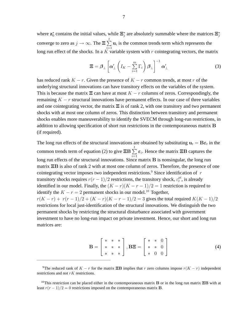
identify the K − r = 2 permanent shocks in our model.10 Together,

r(K − r) + r(r − 1)/2 + (K − r)(K − r − 1)/2 = 3 gives the total required K(K − 1)/2

restrictions for local just-identification of the structural innovations. We distinguish the two

permanent shocks by restricting the structural disturbance associated with government

investment to have no long-run impact on private investment. Hence, our short and long run

matrices are:

B =

∗ ∗ ∗∗ ∗ ∗∗ ∗ ∗

,BΞ =

∗ ∗ 0

∗ ∗ 0

∗ 0 0

(4)

9The reduced rank of K − r for the matrix ΞB implies that r zero columns impose r(K − r) independent

restrictions and not rK restrictions.

10This restriction can be placed either in the contemporaneous matrix B or in the long run matrix ΞB with at

least r(r − 1)/2 = 0 restrictions imposed on the contemporaneous matrix B.

8

III. DATA

Our baseline specification involves annual Indian data on GDP, public and private sector gross

fixed capital formation for the period 1950-2012.11 The data is from National Account

Statistics as published by the Indian Central Statistical Office. All the variables are measured

in real per capita terms (in 2004-05 prices).

The quarterly frequency data is from the CapEx database of the Centre for Monitoring of

Indian Economy (CMIE), which has been monitoring India’s investment activity since its

creation in 1976. The CapEx database provides systematic coverage of investment projects

that entail a capital expenditure of 10 million rupees or more, beginning in 1996 and

comprising about 45,000 projects. As there is no one source for investment-projects

information, the CapEx data is compiled from all available credible sources. However, this

data should not be seen as comprehensive or perfect in its coverage.

We aggregate project-level costs into quarterly time-series for sector- and industry-level

investment activity. Given the lack of data on actual quarterly spending profiles, we estimate

the quarterly investment activity on the basis of project-level information on total costs and

various project events, such as dates of announcement, implementation, obtainment of

regulatory clearances, completion, abandonment, etc. For projects that have been completed,

the total project cost is apportioned into cash flow on the basis of the length of time between

beginning of a project and its completion. For current investment and abandoned or shelved

projects, the expected duration is based on the average length of comparable investment

undertakings with regard to economic sector and industry (those that have been completed). In

addition, we time-allocate cash flow across periods on the basis of equal discounted cash flow

using the economy-wide investment cost trends (using gross fixed capital formation deflators).

Nonetheless, using this methodology we are not able to account for cost overruns or savings.

For each sector and industry, we construct two measures of investment spending that differ

with respect to treatment of abandoned and shelved investments. The first measure includes

estimated investment spending on such projects up to the point that investment was declared

abandoned or shelved. The second measure assigns zero spending to such projects. The latter

measure thus narrows investment activity only to projects that are more likely to directly make

up a productive capital stock capacity. Given that we are not able to isolate current

investments that may eventually become abandoned or shelved, robustness checks with a

trimmed end-point were conducted.12

11All variables are national aggregates.

12The correlation between the new series (on an annual basis) with public and private gross fixed capital for-

mation from National Accounts Statistics is 0.95 over the period 1995-2012.

9

IV. EMPIRICAL FINDINGS

This section discusses the results of models with annual frequency as well of those with

quarterly investment data. Our baseline specification (hereafter Model 1) contains annual data

on yt, git, and pit over the period 1950-2012 (63 observations). We treat this specification as

the baseline to enable comparison with earlier studies like Mitra (2006) and Serven (1999),

which also used annual data on roughly comparable (though shorter) samples. We also check

whether private investment responds differently to accumulation of public infrastructure

capital like electricity, railways, other transport, and communication, while keeping the

sample period and identification strategy unchanged. Accounting for this heterogeneity is

important as public infrastructure projects can raise the profitability of private production and

thereby encourage private investment. To test this hypothesis, we estimate Model 2 with

variables yt, giinfrt , and pit, where giinfr

t denotes investment in infrastructure sectors.13

Columns 1 and 2 of Table 3 report the estimated loading coefficients and cointegrating vectors

respectively. The α and β vectors of Models 1 and 2 are reported in rows 1 and 2,

respectively.14 Although a discussion of causality cannot be made on the basis of

cointegrating vectors alone, it is reassuring to observe that the estimated coefficients on public

and private investment have the theoretically-correct sign in both models. The estimated long

run relationships in both models underline a positive relation between output, public and

private investment. Next we identify Models 1 and 2 based on these long run restrictions as

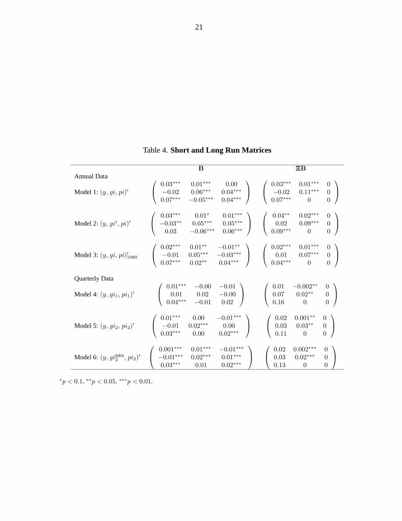
discussed in section 2. The zeros in the BΞ matrix are the long run identification restrictions.

The estimated short (B) and long run (BΞ) matrices of Models 1 and 2 are reported in rows 1

and 2 of table 4, respectively. Given the ordering of the variables, (y, gi, pi)′ and (y, gii, pi)′

respectively, we observe that a structural innovation in public investment crowds out private

investment in the short run in both models. The effect on output due to εgit on the other hand is

positive and statistically significant in both models on impact as well as in the long run.15

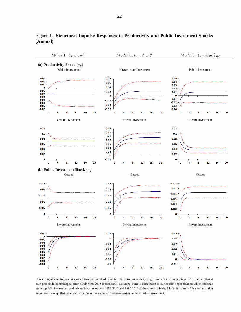
Figure 1, columns 1 and 2, shows the corresponding impulse responses of variables to one

standard deviation shocks in productivity and public investment.

For Model 1, as can be seen from the Panel (a) of Figure 1, the impact of a productivity shock

on public investment is not significantly different from zero over both the short-term and the

long run, while the response of private investment to a productivity shock is significantly

positive, both on impact and over the long run. Panel (b) shows the response of output and

private investment to a structural innovation in public investment. As the graphs show, the

13The industry-wise investment data does not disaggregate data into public and private sector. Therefore we

focus on the industries where most of the investment in the sample period came from the public sector.

14The coefficients corresponding to output in the cointegrating vectors are normalized to one.

15Note that the long run impact of private investment to εgi is already restricted to zero.

10

response of output is positive throughout, while private investment is shown to be temporarily

crowded out by public investment. This response is statistically significant for the first 3 years

after the shock; thereafter the long run response converges to zero.

The impulse responses of Model 2, reported in column 2 of Figure 1, are very similar to those

of Model 1. Here giinfrt does not respond significantly to a productivity shock, while private

investment’s response is positive and significantly different from zero (after 1 year), and

grows over time. The response of output is also very comparable to that reported in column 1.

Most importantly, the crowding out result for private investment in response to a shock in

public infrastructure investment stands as compared to Model 1.

Overall, the results of Models 1 and 2 suggest that over the whole sample, 1950-2012, public

capital accumulation crowds out private investment in the short run. Furthermore, we do not

find any significant differences if we focus our attention only on public investment in

infrastructure. This may be because large investment efforts of the public sector over the last

three decades were concentrated on infrastructure capital in areas such as agricultural

irrigation, transport, telecommunications and power, so the results of Model 2 are very similar

to those of Model 1 with aggregate public investment.

These findings are not surprising, as India relied on a state-led, inward-oriented growth

strategy for more than three decades post independence. A key component of this strategy

was rapid industrialization based on capital-intensive industries, guided by the central plans of

government, see Serven (1999) for details. The comprehensive licensing of firms’ entry,

expansion and diversification plans; reservation of entire productive sectors for the state; high

barriers to foreign trade and investment protecting domestic production from external

competition; and mandatory credit allocation schemes imposed on the banking system were

key components of this strategy, as noted by Serven (1999).

To understand the magnitude of crowding out in our baseline specification, we compute

interim multipliers after one, two, and three years for private sector investment in response to

a one rupee increase in public investment.16 A one rupee increase in public investment is

shown to crowd out private investment by 0.60, 0.31, and 0.17 rupees after one, two, and three

years, respectively. Overall, our baseline results of crowding out in the short run are close to

those obtained in past studies by Mitra (2006) and Serven (1999); both of whom report similar

short run dynamics.

Although the analysis in Models 1 and 2 is useful to compare with similar earlier studies, it

does not acknowledge the substantial structural changes that the Indian economy has

undergone during the past three decades. Starting from late 1970s and throughout the 1980s,

16To calculate the multipliers, we first compute the elasticities of private investment to public investment εpigiover the three years, and divide them by the average ratio of government to private investment over the whole

sample.

11

the Indian economy witnessed reforms in industrial and trade policies. These included

deregulation of the domestic market which implied loosening of restrictions on entry,

expansion and output mix. Trade reforms were aimed at reducing quantitative controls on

import goods, resulting in availability of high quality machinery and capital goods.

Furthermore, the 1991 liberalization process marked a complete restructuring of major policy

areas, see Ahluwalia (2002) among others. License restrictions were abolished and all except

a few industries were made open to the private sector. Import quotas were eliminated and

there was a substantial reduction in tariff rates. Monetary policy focused on price stability and

availability of credit to investors. There was a substantial easing of restrictions on the banking

sector including a reduction of the cash reserve ratio (CRR) and the statutory liquidity ratio

(SLR). Correspondingly, empirical studies on India generally highlight two key structural

breaks in the growth rate of GDP. While Rodrik and Subramanian (2005) and DeLong (2003)

report a break in 1980s, Ahluwalia (2002) (among others) attribute the break to 1990s due to

the economic reforms following the 1991 balance of payments crisis.

We examine whether the response of private investment to public capital accumulation has

changed in the latter half of our sample. We first check for the existence of a break during the

period 1975-2000 in our sample, using Chow break-point and Chow-forecast tests.17 Instead

of choosing a single break date, we perform the test assuming the break-point to be anytime

between 1975-2000 and repeat the test for each year in the sample. For both tests, the null is

of parameter constancy and high test statistics result in the rejection of the null. We use 2000

bootstrapped replications to compute the p-values for the tests. The results indicate that the

null of parameter constancy is rejected for a range of years during 1975-2000, which provides

evidence towards a true underlying break in the model. We select 1980 as the year of the

break as it corresponds to the year that gives the highest values of the break-point and

split-sample test statistics. Without rejecting the possibility of a second break in early 1990s,

we find strong evidence of a break around 1980, in agreement with the findings of Rodrik and

Subramanian (2005) among others.18

With evidence of a break point in 1980, we re-estimate Model 3 in yt, git, and pit over

1980-2012. The estimated loading and cointegrating vectors are reported in row 3 of Table 3,

while the short and long run matrices are reported in row 3 of Table 4. The impulse responses

are shown in Figure 1, column 3. The graphs show that the response of public and private

investment to productivity shocks, and the output response to a public investment shock, are

very similar to Model 1 (column 1). However, the response of private investment to public

capital accumulation differs significantly from earlier specifications. In this specification, a

policy-induced increase in public investment significantly crowds in private investment in the

17They test the stability of the parameters of model as a whole.

18Our analysis of unit root test with two structural breaks as discussed in Clemente et al. (1998) shows breaks

in 1983-1984 for y, gi, and pi. A second break is also indicated for y and pi at 1996.

12

short run. The calculated interim multipliers are 0.37, 0.16, and 0.07 after the first, second,

and third years, respectively. This exercise, therefore, indicates that public capital

accumulation may have become more complementary to private investment since the early

1980s.

A. Quarterly analysis using post-liberalization data

While Rodrik and Subramanian (2005) argue that the pickup in India’s economic growth

preceded the 1991 liberalization by a full decade, there is a consensus in the literature on the

role of pro-market reforms of 1990s in transforming the Indian economy. Spurred by a

balance of payments crisis in 1991, Indian policy-makers began liberalizing the economy by

slashing trade barriers, attracting foreign investment, dismantling the license raj regime, and

beginning privatization. The economy started to boom afterwards and graduated from the

so-called "Hindu rate of growth". This section investigates whether the relationship between

public and private investment has changed after these policy reforms.

We again use the CapEx-CMIE database to construct the quarterly series of public and private

investment in India. As we discussed in the data section, we construct two alternative

measures of investment: type 1 which counts investment projects even for failed ones (i.e.

where investment is counted until the project is either completed, shelved, or abandoned); and

type 2 which simply does not consider failed projects in the construction of the two investment

series. Model 4 corresponds to the case where the investment series are constructed as type 1,

gi1t and pi1t for public and private sectors, respectively. Model 5 considers investment series

calculated as type 2. We treat Model 5 as our preferred specification because type 2 series

abstract from making any assumptions on the investment-flow from projects that possibly

never started. Finally, analogous to the exercise in annual data, Model 6 replaces gi2t with

gi2,infrat where gi2,infra

t is the public investment series on infrastructure sectors.

Rows 4, 5, and 6 of Table 3 report the loading coefficients and cointegrating vectors

corresponding to Models 4, 5, and 6, respectively. The signs of estimated coefficients on

public and private investment in the long run relationships are broadly as expected but smaller

in magnitude than those obtained in annual data estimations.19 The estimated short and long

run matrices B and BΞ for the three models are reported in rows 4, 5, and 6 of Table 4. The

corresponding impulse responses are shown in columns 1, 2 and 3 of Figure 2. As row 1 of

Figure 2 shows, for all the 3 specifications, the response of public investment to a productivity

shock is positive and statistically significant after 4-6 quarters. Similar to the impulse

responses in annual data, the response of private investment (row 2) to a productivity shock is

19The relatively smaller size of the coefficients in comparison to the annual results may be due to the higher

frequency of data in Models 4-6. Also, the investment series constructed using investment-project announcements

are only proxies for the actual investment activities.

13

also positive and statistically significant in all the models. The response of output to a

policy-induced change in public investment (panel b) is not significantly different from zero in

the first 8 quarters in Model 4. However, there is a statistically significant positive impact on

output from a public investment shock over the first 8 quarters in Models 5 and 6 (which

continue to be small and positive in the long run).

Finally, the impulse responses of private investment to a structural innovation in government

investment are reported in the last row of Figure 2. Reassuringly and in agreement with the

earlier results from Model 3, none of the three quarterly specifications predict crowding out of

private investment. On the contrary, under our preferred specification, Model 5, there is

evidence for a positive and significant crowding in of private investment by public sector

investment from quarters eight to twelve. Computing interim multipliers using Model 5, we

find that a one rupee increase in public investment crowds in private investment by 0.30, 1.24,

and 1.07 rupees after four, eight, and twelve quarters, respectively. The response of private

investment to public infrastructure investment shocks (last graph) is very similar to the case

when aggregate public investment is considered (second graph, last row).

Overall, there is evidence for "crowding in" of private investment by public investment, once

we restrict the sample post 1980. Similar responses of private investment to a public capital

accumulation shock over Models 3, 4, 5, and 6 suggest that public investment has been

complementary to the activities of the private sector over both 1980-2012 or 1996Q2-2015Q1

periods. In retrospect, the crowding in finding is not very surprising given the huge

infrastructure deficit in India, but it has not been usually found previously in the Indian

empirical literature, see Mitra (2006) and Serven (1999). Furthermore, the standard arguments

for crowding out (assuming that the economy is operating on its production possibility

frontier and has developed financial markets) do not appear to hold for emerging market

economies like India. In fact, the crowding out of private investment by public investment

over the full sample is likely a reflection of a state-led, inward-oriented growth strategy that

existed before the 1980s, which was not supportive of private sector investment.

V. CONCLUDING REMARKS

Acknowledging the importance of key structural changes that happened in the Indian

economy during 1980s and early 1990s, and their potential impact on the relationship

between public and private investment, we estimated a variety of SVECMs over different

sample periods and frequencies to examine the presence or absence of investment crowding in

(out) in India. We embedded (and tested) a long-term relationship between output, public and

private investment (motivated by the stationarity of the "great ratio" of aggregate investment

and output). We used the properties of the theory-driven long-term relationship to decompose

the structural innovations into those with permanent and temporary effects and to identify the

14

SVECMs. We found public investment "crowded out" private investment in India over the

period 1950-2012. In contrast, we found support for crowding in of private investment over

the more recent period of 1980-2012. This change in the relationship can be attributed to the

policy reforms which started during early 1980s and gained momentum after the 1991 Indian

balance of payments crisis. This finding of crowding in is further supported by our quarterly

model (estimated over 1996Q2-2015Q1), using project announcements as recorded by

CapEx-CMIE database. Future research can exploit our novel micro dataset of public and

private investment at quarterly frequency to further disentangle the region- or sector-wise

relationship between public investment and private investment in India. For example, one

could examine whether states with policies that are more conducive to private investment

observed more crowding-in. This will have implications for the design of macroeconomic

policies at the level of states or central government.

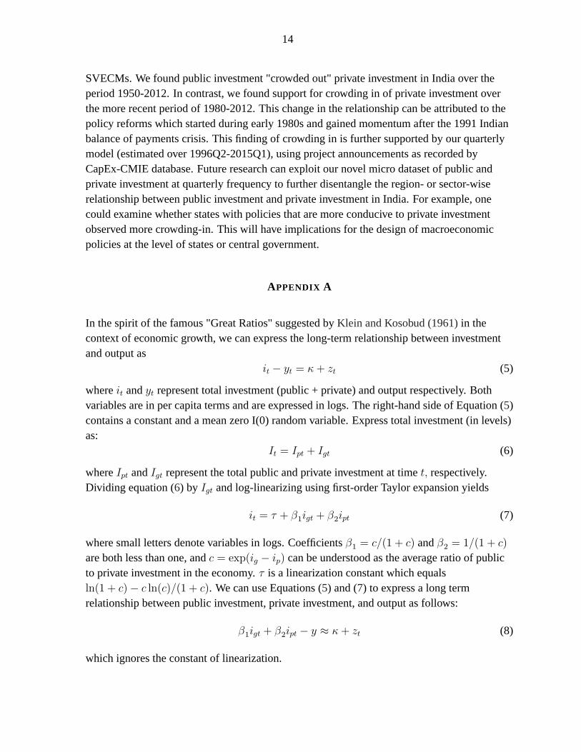
APPENDIX A

In the spirit of the famous "Great Ratios" suggested by Klein and Kosobud (1961) in the

context of economic growth, we can express the long-term relationship between investment

and output as

it − yt = κ+ zt (5)

where it and yt represent total investment (public + private) and output respectively. Both

variables are in per capita terms and are expressed in logs. The right-hand side of Equation (5)

contains a constant and a mean zero I(0) random variable. Express total investment (in levels)

as:

It = Ipt + Igt (6)

where Ipt and Igt represent the total public and private investment at time t, respectively.

Dividing equation (6) by Igt and log-linearizing using first-order Taylor expansion yields

it = τ + β1igt + β2ipt (7)

where small letters denote variables in logs. Coefficients β1 = c/(1 + c) and β2 = 1/(1 + c)

are both less than one, and c = exp(ig − ip) can be understood as the average ratio of public

to private investment in the economy. τ is a linearization constant which equals

ln(1 + c)− c ln(c)/(1 + c). We can use Equations (5) and (7) to express a long term

relationship between public investment, private investment, and output as follows:

β1igt + β2ipt − y ≈ κ+ zt (8)

which ignores the constant of linearization.

15

APPENDIX B

Unit root tests

We first determine the order of integration of the variables yt, git, pit, and giinfrt over the

period 1950-2012. We report the results from the Augmented Dickey-Fuller (ADF) test,

ADF-GLS test as proposed by Elliott et al. (1996), and Phillips-Perron (PP) unit root test. All

three tests have a null hypothesis of individual series being a random walk against the

alternative of stationarity. To preserve uniformity across tests, we select the lag order for a

variable based on Ng–Perron modified Akaike information criterion (MAIC) as reported in

the ADF-GLS test. Since all variables, when expressed in levels, appear to be trending, all

tests on the level of variables include a deterministic time trend.20 The results are reported in

the first panel of Table 1. They indicate that we cannot reject the null of non-stationarity even

at 10% level, while all the tests on the first-differenced variables strongly reject the presence

of a unit root at 1% significance level. We therefore conclude that all four variables are

integrated of order 1 or I(1).21 Similarly, all variables are shown to be integrated of order one

over the smaller sub-sample from 1980 (panel 2). Finally, we test for unit roots in quarterly

series where we have two variants of public and private investment, as discussed in the data

section. For all variables, the null of a unit root cannot be rejected even at 10% level of

significance, while all variables except pi1 and pi2 clearly reject the null of a unit root in first

differences. Although for pi1 and pi2, the null of unit root cannot be rejected in first

differences for ADF test, the Phillips–Perron test strongly rejects the null at the 1% level. We

therefore continue to treat pi1 and pi2 as I(1).

Cointegration rank tests

Table 2 reports the lag order and the number of cointegrating vectors used in various VECM

models discussed in the paper. For all specifications using annual data, a VECM order of 0 (in

first differences) is selected based on the Akaike Information Criterion.22 Models 1 and 2,

which are based on the full sample data confirm the presence of one cointegrating vector

based on 99% trace test statistic. Although Model 3 does not confirm the presence of any

cointegration between the three variables, this may be due to the loss of power of the test over

a small sample of around 30 annual observations. For robustness, we conduct the Johansen

trace test with structural break as discussed in Johansen et al. (2000) where we take yt, git,

and pit over the whole sample, but allow for breaks in level and trend at 1980. The test

20No trend is included in the tests on first-differenced variables.

21As a robustness check to our unit root tests, we also conducted the Clemente et al. (1998) unit root test, which

allows for one or two structural breaks in the series being tested for non-stationarity. Our results (available on

request) are robust to this additional test.

22Maximum number of lags were set to two years.

16

strongly supports the evidence of one cointegrating vector. The results do not change even if

we allow for a second break in 1991. Hence, we continue to estimate a VECM with one

cointegration rank in Model 3. For VECMs using quarterly data, a lag order of 7 (in first

differences) is selected based on the Akaike Information Criterion.23 Models 4 and 6, using

quarterly data, support the presence of one cointegrating relation between the three variables.

Model 5 indicates the presence of two cointegrating vectors. However, we continue to

proceed with one cointegrating rank which is also confirmed by maximum eigen value test

statistic at the same significance level (not reported in the paper but available upon request).

REFERENCES

Ahluwalia, M. S. (2002). Economic Reforms in India Since 1991: Has Gradualism Worked?

Journal of Economic Perspectives 16(3), 67–88.

Aschauer, D. A. (1989a). Does Public Capital Crowd Out Private Capital? Journal of

Monetary Economics 24(2), 171 – 188.

Aschauer, D. A. (1989b). Is Public Expenditure Productive? Journal of Monetary

Economics 23(2), 177 – 200.

Binder, M. and M. Pesaran (1999). Stochastic Growth Models and Their Econometric

Implications. Journal of Economic Growth 4(2), 139–183.

Blanchard, O. and R. Perotti (2002). An Empirical Characterization of the Dynamic Effects

of Changes in Government Spending and Taxes on Output. The Quarterly Journal of

Economics 117(4), 1329–1368.

Blanchard, O. J. and D. Quah (1989). The Dynamic Effects of Aggregate Demand and

Supply Disturbances. The American Economic Review 79(4), pp. 655–673.

Blejer, M. I. and M. S. Khan (1984). Government Policy and Private Investment in

Developing Countries. Staff Papers (International Monetary Fund) 31(2), pp. 379–403.

Breitung, J., R. Brüggemann, and H. Lütkepohl (2004). Structural vector autoregressive

modeling and impulse responses. In H. Lütkepohl and M. Krätzig (Eds.), Applied Time

Series Econometrics, pp. 159–195. Cambridge University Press.

Cashin, P. (1995). Government Spending, Taxes, and Economic Growth. Staff

23Only for Model 6, AIC reports lag of 8, while FPE reports lag order 6. To maintain uniformity of lags across

models 4, 5, and 6, we continue to choose lag 7 as before. Results are invariant to the inclusion of lag order 8 for

model 6.

17

Papers-International Monetary Fund, 237–269.

Chudik, A., K. Mohaddes, M. H. Pesaran, and M. Raissi (2015a). Long-Run Effects in Large

Heterogeneous Panel Data Models with Cross-Sectionally Correlated Errors. Federal

Reserve Bank of Dallas, Globalization and Monetary Policy Institute Working Paper

No. 223.

Chudik, A., K. Mohaddes, M. H. Pesaran, and M. Raissi (2015b). Is There a Debt-threshold

Effect on Output Growth? forthcoming in Review of Economics and Statistics.

Clemente, J., A. Montañés, and M. Reyes (1998). Testing for a Unit Root in Variables with a

Double Change in the Mean. Economics Letters 59(2), 175 – 182.

DeLong, J. B. (2003). India since independence: An analytic growth narrative. In D. Rodrik

(Ed.), In Search of Prosperity. Princeton University Press.

Elliott, G., T. J. Rothenberg, and J. H. Stock (1996). Efficient Tests for an Autoregressive

Unit Root. Econometrica 64(4), pp. 813–836.

Erden, L. and R. G. Holcombe (2005). The Effects of Public Investment on Private

Investment in Developing Economies. Public Finance Review 33(5), 575–602.

Evans, P. and G. Karras (1994). Are Government Activities Productive? Evidence from a

Panel of U.S. States. The Review of Economics and Statistics 76(1), pp. 1–11.

Gali, J. (1999). Technology, Employment, and the Business Cycle: Do Technology Shocks

Explain Aggregate Fluctuations? American Economic Review 89(1), 249–271.

Garratt, A., K. Lee, M. H. Pesaran, and Y. Shin (2012). Global and National

Macroeconometric Modelling: a Long-Run Structural Approach. Oxford University

Press.

Gonzalo, J. and S. Ng (2001). A Systematic Framework For Analyzing the Dynamic Effects

of Permanent and Transitory Shocks. Journal of Economic Dynamics and

Control 25(10), 1527 – 1546.

Greene, J. and D. Villanueva (1991). Private Investment in Developing Countries: An

Empirical Analysis. Staff Papers (International Monetary Fund) 38(1), pp. 33–58.

Johansen, S., R. Mosconi, and B. Nielsen (2000). Cointegration Analysis in the Presence of

Structural Breaks in the Deterministic Trend. The Econometrics Journal 3(2), pp.

216–249.

Jones, C. I. (1995). R & D-Based Models of Economic Growth. Journal of Political

18

Economy 103(4), pp. 759–784.

Kilian, L. (2013). Structural Vector Autoregressions. In N. Hashimzade and M. A. Thornton

(Eds.), Handbook of Research Methods and Applications in Empirical

Macroeconomics, Chapter 22, pp. 515–554. Edward Elgar Publishing.

King, R. G., C. I. Plosser, J. H. Stock, and M. W. Watson (1991). Stochastic Trends and

Economic Fluctuations. The American Economic Review 81(4), pp. 819–840.

Klein, L. R. and R. F. Kosobud (1961). Some Econometrics of Growth: Great Ratios of

Economics. The Quarterly Journal of Economics 75(2), pp. 173–198.

Kocherlakota, N. R. and K.-M. Yi (1996). Simple Time Series Test of Endogenous vs.

Exogenous Growth Models: An Application to the United States. The Review of

Economics and Statistics 78(1), pp. 126–134.

Mitchell, D. J. (2000). The Importance of Long Run Structure for Impulse Response

Analysis in VAR Models. NIESR Discussion Paper no. 172, 337–341.

Mitra, P. (2006). Has Government Investment Crowded Out Private Investment in India?

American Economic Review 96(2), 337–341.

Pagan, A. and M. H. Pesaran (2008). Econometric Analysis of Structural Systems with

Permanent and Transitory Shocks. Journal of Economic Dynamics and Control 32(10),

3376 – 3395.

Rodrik, D. and A. Subramanian (2005). From "Hindu Growth" to Productivity Surge: The

Mystery of the Indian Growth Transition. IMF Staff Papers 52(2), pp. 193–228.

Serven, L. (1999). Does Public Capital Crowd Out Private Capital? Evidence from India.

19

Table 1. Unit Root Tests

Annual Data 1950-2012

y gi pi giinfra

ADF 1.15 −2.98 −0.31 −1.23ADF-GLS 0.16 −1.61 −0.76 −1.30PP 1.02 −2.55 −1.28 −0.86

∆y ∆gi ∆pi ∆giinfra

ADF −6.88∗∗∗ −5.66∗∗∗ −4.40∗∗∗ −6.35∗∗∗

ADF-GLS −6.54∗∗∗ −5.70∗∗∗ −2.39∗∗ −6.00∗∗∗

PP −6.88∗∗∗ −5.71∗∗∗ −7.81∗∗∗ −6.35∗∗∗

Annual Data 1980-2012

y gi piADF −0.58 −0.53 −2.07ADF-GLS −0.68 −0.85 −1.49PP −0.37 −0.47 −3.02

∆y ∆gi ∆piADF −4.32∗∗∗ −4.48∗∗∗ −3.66∗∗

ADF-GLS −4.40∗∗∗ −4.45∗∗∗ −3.63∗∗

PP −4.32∗∗∗ −4.48∗∗∗ −6.98∗∗∗

Quarterly Data 1996Q2-2015Q1

y gi1 pi1 gi2 pi2 giinfra2

ADF −1.99 −2.32 −2.70 −1.71 −2.46 −1.38ADF-GLS −1.27 −1.86 −2.10 −1.09 −1.89 −1.37PP −2.47 −1.42 −1.66 −1.45 −1.83 −1.96

∆y ∆gi1 ∆pi1 ∆gi2 ∆pi2ADF −9.14∗∗∗ −2.81∗ −2.01 −6.20∗∗∗ −2.06 −0.80ADF-GLS −4.54∗∗∗ −2.82∗∗∗ −1.97∗ −6.11∗∗∗ −1.73 −3.77∗∗∗

PP −9.14∗∗∗ −5.82∗∗∗ −4.72∗∗∗ −6.20∗∗∗ −5.72∗∗∗ −6.37∗∗∗

∗p < 0.1, ∗∗p < 0.05, ∗∗∗p < 0.01. ADF denotes the Augmented Dickey-Fuller Test, ADF-GLS the generalized

least squares version of the ADF test, and PP the Phillips-Perron test. Trend and intercept are included as deter-

ministic terms in tests with level variables while only intercept is included in tests with differenced variables. For

each variable, the number of lags are selected on Ng–Perron modified Akaike information criterion (MAIC) as

reported in ADF-GLS.

20

Table 2. Lag Orders and Cointegrating Rank of the VECMs

Annual Data

VECM Cointegrating

Order* relations

Model 1: (y, gi, pi)′ 0 1Model 2: (y, gii, pi)′ 0 1Model 3: (y, gi, pi)′1980 0 0

Quarterly Data

VECM Cointegrating

Order* relations

Model 4: (y, gi1, pi1)′ 7 1

Model 5: (y, gi2, pi2)′ 7 2

Model 6: (y, giinfra2 , pi2)

′ 7 1

Notes: * denotes lag order in first differences selected by the Akaike Information Criterion, with the maximum

lag orders set to 2 in models with annual data and 8 in models with quarterly data (see Appendix B for details).

Selection of the number of cointegrating relations is based on the trace test statistics calculated at 99% critical

values.

Table 3. Loading Coefficients and Cointegrating Vectors

α′ β′

Annual Data

Model 1: (y, gi, pi)′(

0.001 0.76∗∗∗ 0.71∗∗∗) (

1 −0.12∗∗∗ −0.44∗∗∗)

Model 2: (y, gii, pi)′(

0.16∗∗ 0.70∗∗∗ 0.90∗∗∗) (

1 −0.20∗∗∗ −0.35∗∗∗)

Model 3: (y, gi, pi)′1980(−0.11 −0.52∗∗ 0.76∗∗

) (1 −0.13∗ −0.65∗∗∗

)Quarterly Data

Model 4: (y, gi1, pi1)′ (

−0.74∗∗∗ −0.10 1.73∗∗) (

1 0.07∗∗ −0.12∗∗∗)

Model 5: (y, gi2, pi2)′ (

−0.25∗∗∗ 0.15 0.97∗∗∗) (

1 −0.03 −0.13∗∗∗)

Model 6: (y, giinfra2 , pi2)

′ (−0.24∗∗∗ 0.37∗∗ 0.99∗∗∗

) (1 −0.03 −0.13∗∗∗

)∗p < 0.1, ∗∗p < 0.05, ∗∗∗p < 0.01.

21

Table 4. Short and Long Run Matrices

B ΞBAnnual Data

Model 1: (y, gi, pi)′

0.03∗∗∗ 0.01∗∗∗ 0.00−0.02 0.06∗∗∗ 0.04∗∗∗

0.07∗∗∗ −0.05∗∗∗ 0.04∗∗∗

0.03∗∗∗ 0.01∗∗∗ 0−0.02 0.11∗∗∗ 00.07∗∗∗ 0 0

Model 2: (y, gii, pi)′

0.03∗∗∗ 0.01∗ 0.01∗∗∗

−0.03∗∗ 0.05∗∗∗ 0.05∗∗∗

0.03 −0.06∗∗∗ 0.06∗∗∗

0.04∗∗ 0.02∗∗∗ 00.02 0.09∗∗∗ 0

0.09∗∗∗ 0 0

Model 3: (y, gi, pi)′1980

0.02∗∗∗ 0.01∗∗ −0.01∗∗

−0.01 0.05∗∗∗ −0.03∗∗∗

0.07∗∗∗ 0.02∗∗ 0.04∗∗∗

0.02∗∗∗ 0.01∗∗∗ 00.01 0.07∗∗∗ 0

0.04∗∗∗ 0 0

Quarterly Data

Model 4: (y, gi1, pi1)′

0.01∗∗∗ −0.00 −0.010.01 0.02 −0.00

0.04∗∗∗ −0.01 0.02

0.01 −0.002∗∗ 00.07 0.02∗∗ 00.16 0 0

Model 5: (y, gi2, pi2)′

0.01∗∗∗ 0.00 −0.01∗∗∗

−0.01 0.02∗∗∗ 0.000.03∗∗∗ 0.00 0.02∗∗∗

0.02 0.001∗∗ 00.03 0.03∗∗ 00.11 0 0

Model 6: (y, giinfra2 , pi2)

′

0.001∗∗∗ 0.01∗∗∗ −0.01∗∗∗

−0.01∗∗∗ 0.02∗∗∗ 0.01∗∗∗

0.03∗∗∗ 0.01 0.02∗∗∗

0.02 0.002∗∗∗ 00.03 0.02∗∗∗ 00.13 0 0

∗p < 0.1, ∗∗p < 0.05, ∗∗∗p < 0.01.

22

Figure 1. Structural Impulse Responses to Productivity and Public Investment Shocks

(Annual)

Model 1 : (y, gi, pi)′ Model 2 : (y, gii, pi)′ Model 3 : (y, gi, pi)′1980

(a) Productivity Shock (εy)Public Investment Infrastructure Investment Public Investment

Private Investment Private Investment Private Investment

(b) Public Investment Shock (εg)Output Output Output

Private Investment Private Investment Private Investment

Notes: Figures are impulse responses to a one standard deviation shock to productivity or government investment, together with the 5th and

95th percentile bootstrapped error bands with 2000 replications. Columns 1 and 3 correspond to our baseline specification which includes

output, public investment, and private investment over 1950-2012 and 1980-2012 periods, respectively. Model in column 2 is similar to that

in column 1 except that we consider public infrastructure investment instead of total public investment.

23

Figure 2. Structural Impulse Responses to Productivity and Public Investment Shocks

(Quarterly)

Model 4 : (y, gi1, pi1)′ Model 5 : (y, gi2, pi2)

′ Model 6 : (y, giinfra2 , pi2)

′

(a) Productivity Shock (εy)Public Investment Public Investment Public Investment

Private Investment Private Investment Private Investment

(b) Public Investment Shock (εg)Output Output Output

Private Investment Private Investment Private Investment

Notes: Figures are impulse responses to a one standard deviation shock to productivity or public investment, together with the 5th and 95th

percentile bootstrapped error bands with 2000 replications. The impulse responses correspond to models with quarterly data on public and

private investment projects constructed from CAPEX-CMIE database. Columns 1, 2, and 3 show impulse responses of models 4, 5, and

6, respectively. In model 4, shelved or abandoned projects (for both public and private sectors) are not included in the construction of the

investment series once they are shelved or abandoned. Model 5 considers the other extreme where shelved or abandoned projects are not

excluded from the investment series altogether from the date of announcement. Model 6 takes public investment as constructed in Model 4

and private investment as in Model 5.