Cross-view Embeddings for Information Retrievalusers.dsic.upv.es/~prosso/resources/GuptaPhD.pdf ·...
182
Cross-view Embeddings for Information Retrieval Parth Alokkumar Gupta Departamento de Sistemas Inform´ aticos y Computaci´on Advisor: Dr. Paolo Rosso Universitat Polit` ecnica de Val` encia Co-advisor: Dr. Rafael E. Banchs Institute for Infocomm Research, Singapore Thesis developed to obtain the Degree of Doctor por la Universitat Polit` ecnica de Val` encia December, 2016
Transcript of Cross-view Embeddings for Information Retrievalusers.dsic.upv.es/~prosso/resources/GuptaPhD.pdf ·...
Cross-view Embeddings for Information Retrieval
Parth Alokkumar Gupta
Departamento de Sistemas Informaticos y Computacion
Advisor: Dr. Paolo Rosso
Universitat Politecnica de Valencia
Co-advisor: Dr. Rafael E. Banchs
Institute for Infocomm Research, Singapore
Thesis developed to obtain the Degree of
Doctor por la Universitat Politecnica de Valencia
December, 2016

Abstract
In this dissertation, we deal with the cross-view tasks related to information retrieval
using embedding methods. We study existing methodologies and propose new meth-
ods to overcome their limitations. We formally introduce the concept of mixed-script
IR, which deals with the challenges faced by an IR system when a language is written
in different scripts because of various technological and sociological factors. Mixed-
script terms are represented by a small and finite feature space comprised of character
n-grams. We propose the cross-view autoencoder (CAE) to model such terms in an
abstract space and CAE provides the state-of-the-art performance.
We study a wide variety of models for cross-language information retrieval (CLIR)
and propose a model based on compositional neural networks (XCNN) which over-
comes the limitations of the existing methods and achieves the best results for many
CLIR tasks such as ad-hoc retrieval, parallel sentence retrieval and cross-language
plagiarism detection. We empirically test the proposed models for these tasks on
publicly available datasets and present the results with analyses.
In this dissertation, we also explore an effective method to incorporate contextual
similarity for lexical selection in machine translation. Concretely, we investigate a
feature based on context available in source sentence calculated using deep autoen-
coders. The proposed feature exhibits statistically significant improvements over the
strong baselines for English-to-Spanish and English-to-Hindi translation tasks.
i
ii Abstract
Finally, we explore the the methods to evaluate the quality of autoencoder gen-
erated representations of text data and analyse its architectural properties. For this,
we propose two metrics based on reconstruction capabilities of the autoencoders:
structure preservation index (SPI) and similarity accumulation index (SAI). We also
introduce a concept of critical bottleneck dimensionality (CBD) below which the
structural information is lost and present analyses linking CBD and language per-
plexity.
Resumen
En esta disertacion estudiamos problemas de vistas-multiples relacionados con la re-
cuperacion de informacion utilizando tecnicas de representacion en espacios de baja
dimensionalidad. Estudiamos las tecnicas existentes y proponemos nuevas tecnicas
para solventar algunas de las limitaciones existentes. Presentamos formalmente el
concepto de recuperacion de informacion con escritura mixta, el cual trata las difi-
cultades de los sistemas de recuperacion de informacion cuando los textos contienen
escrituras en distintos alfabetos debido a razones tecnologicas y socioculturales. Las
palabras en escritura mixta son representadas en un espacio de caracterısticas finito y
reducido, compuesto por n-gramas de caracteres. Proponemos los auto-codificadores
de vistas-multiples (CAE, por sus siglas en ingles) para modelar dichas palabras en
un espacio abstracto, y esta tecnica produce resultados de vanguardia.
En este sentido, estudiamos varios modelos para la recuperacion de informacion
entre lenguas diferentes (CLIR, por sus siglas en ingles) y proponemos un modelo
basado en redes neuronales composicionales (XCNN, por sus siglas en ingles), el cual
supera las limitaciones de los metodos existentes. El metodo de XCNN propuesto
produce mejores resultados en diferentes tareas de CLIR tales como la recuperacion
de informacion ad-hoc, la identificacion de oraciones equivalentes en lenguas distintas
y la deteccion de plagio entre lenguas diferentes. Para tal efecto, realizamos pruebas
experimentales para dichas tareas sobre conjuntos de datos disponibles publicamente,
iii
iv Resumen
presentando los resultados y analisis correspondientes.
En esta disertacion, tambien exploramos un metodo eficiente para utilizar simil-
itud semantica de contextos en el proceso de seleccion lexica en traduccion automatica.
Especıficamente, proponemos caracterısticas extraıdas de los contextos disponibles
en las oraciones fuentes mediante el uso de auto-codificadores. El uso de las ca-
racterısticas propuestas demuestra mejoras estadısticamente significativas sobre sis-
temas de traduccion robustos para las tareas de traduccion entre ingles y espanol, e
ingles e hindu.
Finalmente, exploramos metodos para evaluar la calidad de las representaciones
de datos de texto generadas por los auto-codificadores, a la vez que analizamos
las propiedades de sus arquitecturas. Como resultado, proponemos dos nuevas
metricas para cuantificar la calidad de las reconstrucciones generadas por los auto-
codificadores: el ındice de preservacion de estructura (SPI, por sus siglas en ingles)
y el ındice de acumulacion de similitud (SAI, por sus siglas en ingles). Tambien
presentamos el concepto de dimension crıtica de cuello de botella (CBD, por sus siglas
en ingles), por debajo de la cual la informacion estructural se deteriora. Mostramos
que, interesantemente, la CBD esta relacionada con la perplejidad de la lengua.
Resum
En aquesta dissertacio estudiem els problemes de vistes-multiples relacionats amb
la recuperacio d’informacio utilitzant tecniques de representacio en espais de baixa
dimensionalitat. Estudiem les tecniques existents i en proposem unes de noves per
solucionar algunes de les limitacions existents. Presentem formalment el concepte
de recuperacio d’informacio amb escriptura mixta, el qual tracta les dificultats dels
sistemes de recuperacio d’informacio quan els textos contenen escriptures en diferents
alfabets per motius tecnologics i socioculturals. Les paraules en escriptura mixta son
representades en un espai de caracterıstiques finit i reduıt, composat per n-grames
de caracters. Proposem els auto-codificadors de vistes-multiples (CAE, per les seves
sigles en angles) per modelar aquestes paraules en un espai abstracte, i aquesta
tecnica produeix resultats d’avantguarda.
En aquest sentit, estudiem diversos models per a la recuperacio d’informacio entre
llengues diferents (CLIR , per les sevas sigles en angles) i proposem un model basat
en xarxes neuronals composicionals (XCNN, per les sevas sigles en angles), el qual
supera les limitacions dels metodes existents. El metode de XCNN proposat produeix
millors resultats en diferents tasques de CLIR com ara la recuperacio d’informacio
ad-hoc, la identificacio d’oracions equivalents en llengues diferents, i la deteccio de
plagi entre llengues diferents. Per a tal efecte, realitzem proves experimentals per
aquestes tasques sobre conjunts de dades disponibles publicament, presentant els
v
vi Resum
resultats i analisis corresponents.
En aquesta dissertacio, tambe explorem un metode eficient per utilitzar simil-
itud semantica de contextos en el proces de seleccio lexica en traduccio automatica.
Especıficament, proposem caracterıstiques extretes dels contextos disponibles a les
oracions fonts mitjancant l’us d’auto-codificadors. L’us de les caracterıstiques pro-
posades demostra millores estadısticament significatives sobre sistemes de traduccio
robustos per a les tasques de traduccio entre angles i espanyol, i angles i hindu.
Finalment, explorem metodes per avaluar la qualitat de les representacions de
dades de text generades pels auto-codificadors, alhora que analitzem les propietats
de les seves arquitectures. Com a resultat, proposem dues noves metriques per
quantificar la qualitat de les reconstruccions generades pels auto-codificadors: l’ındex
de preservacio d’estructura (SCI, per les seves sigles en angles) i l’ındex d’acumulacio
de similitud (SAI, per les seves sigles en angles). Tambe presentem el concepte de
dimensio crıtica de coll d’ampolla (CBD, per les seves sigles en angles), per sota de
la qual la informacio estructural es deteriora. Mostrem que, de manera interessant,
la CBD esta relacionada amb la perplexitat de la llengua.
Acknowledgements
First and foremost, I want to express my gratitude for people without whom this
research might not be possible.
My sincere thanks to Paolo Rosso who graciously helped me with every aspect
of this journey. He has devoted a huge amount of time in training me in the field of
research. I am also highly thankful to him because of having confidence in me and
providing me all the opportunities to succeed in this project. The enthusiasm and
trust he has shown to support me is unparalleled. He has been a fantastic advisor.
I thank Rafael E. Banchs, my co-advisor, for the his valuable effort and energy
put in advising me with research. He also played an instrumental part in hosting me
at Institute for Infocomm Research (8 months - Singapore) and introducing me to
the aspects of industrial research. I am also thankful to him for introducing me to
the world of neural networks and helping me to take some critical decisions in terms
of focus of this dissertation.
Thanks to Doug Oard, Lluis Marquez and Pablo Castell, who have given their
feedback as external reviewers. Their constructive and insightful comments have
greatly improved the quality of this dissertation. I also thank Eneko Agirre, Julio
Gonzalo and Jaap Kamps to be on the thesis defense committee.
I feel lucky to work with colleagues at PRHLT research center and DSIC like Al-
berto Barron-Cedeno, Enrique Flores, Marc Franco Salvador, Francisco Rangel, Irazu
vii
viii Acknowledgements
Hernandez , Maite Gimenez, Joan Puigcerver and Mauricio Villegas. I also enjoyed
the discussions with Jon Ander Gomez. Roberto Paredes, Francisco Casacuberta
and Enrique Vidal have been very helpful by providing constructive feedback.
This work has also benefited a lot from collaborations with Marta Ruiz Costa-
Jussa from UPC. She has been very helpful and motivating with the aspects related
to machine translation. I want to thank Claudio Giuliano for hosting me at FBK re-
search center (2 months - Italy) and providing constructive feedback on experimental
setup. Collaborations with Monojit Choudhury and Kalika Bali has been very helpful
in this research especially with the mixed-script information retrieval aspect. They
generously hosted me at Microsoft Research (3 months - India). It is also very im-
portant for me to express my gratitude to Doug Oard and Iadh Ounis for providing
me insightful comments on this work in the framework of Doctoral Consortium at
SIGIR (Australia). I am thankful to ACM for providing this opportunity through
ACM Travel Grant. I am very thankful to Nicola Cancedda to mentor me at Mi-
crosoft Bing (4 months - London) and introducing me to the plethora of engineering
challenges involved in research and web search. Jose Santos, Andrea Moro, Daniel
Voinea, Panagiotis Tigas and Bhaskar Mitra at Microsoft Bing have also been very
supportive. I also want to thank Paul Clough, Mark Stevenson, Prasenjit Majumder,
Mandar Mitra for helping in organising CL!NSS and MSIR research tracks at FIRE.
I am also thankful to Shobha L and Vasudev Varma for hosting me at AU-KBC
research center (3 months - Chennai) and IIIT-Hyderabad (2 months) respectively
in the framework of WIQ-EI project.
My sincere gratitude to Neha for believing in me and standing by my side through-
out this journey. The love and support has always been a source of energy. I also
want to thank my parents - Alokkumar Gupta and Mithilesh Gupta - and sister -
Nirzari Gupta - for all the love and blessings. I am very happy that you are proud
of me. I want to thank Rosa and Oreste for making me feel like home in a foreign
country. During this journey, I had a chance to enjoy the friendship of Joan Pastor,
Marcos Calvo, Joaquin Planells, Fernando Sanchez-Vega, Dasha Bogdanova, Ismael
Acknowledgements ix
Diaz. I am also thankful to David Aguilar, Soren Volgmann and Dishant Chauhan
for their friendship. The staff at UPV has been tremendously supportive in every
possible way. The list of people to thank is long and I am sure to have missed some
names.
Finally, my thanks to the Universitat Politecnica de Valencia for supporting the
PhD thesis through Formacion de Personal Investigador (FPI) grant (№ de registro
- 3505). This research has been carried out in the framework of following pro-
jects: (i) WIQ-EI IRSES project (Grant No. 269180) within the FP 7 Marie Curie;
(ii) Text-Enterprise 2.0 research project (TIN2009-13391-C04-03); and (iii) DIANA-
APPLICATIONS - Finding Hidden Knowledge in Texts: Applications (TIN2012-
38603-C02-01). I gratefully acknowledge the support of NVIDIA Corporation with
the donation of the GeForce Titan GPU used for this research.

Contents
Abstract i
Resumen iii
Resum v
Acknowledgements vii
Contents xi
List of Figures xvii
List of Tables xix
1 Introduction 1
1.1 Contributions . . . . . . . . . . . . . . . . . . . . . . . . . . . . . . . 3
1.1.1 Mixed-script information retrieval . . . . . . . . . . . . . . . . 3
1.1.2 Cross-view models . . . . . . . . . . . . . . . . . . . . . . . . 5
1.1.3 Critical bottleneck dimensionality . . . . . . . . . . . . . . . . 6
1.2 Research Questions (RQ) . . . . . . . . . . . . . . . . . . . . . . . . . 6
1.3 Outline of the dissertation . . . . . . . . . . . . . . . . . . . . . . . . 7
xi
xii CONTENTS
2 Theoretical background 9
2.1 Information retrieval (IR) . . . . . . . . . . . . . . . . . . . . . . . . 9
2.1.1 Vector space model . . . . . . . . . . . . . . . . . . . . . . . . 10
2.1.2 Indexing and retrieval . . . . . . . . . . . . . . . . . . . . . . 11
2.1.3 Evaluation . . . . . . . . . . . . . . . . . . . . . . . . . . . . . 12
2.1.4 Semantic term-relatedness . . . . . . . . . . . . . . . . . . . . 14
2.2 Dimensionality reduction . . . . . . . . . . . . . . . . . . . . . . . . . 15
2.3 IR across languages . . . . . . . . . . . . . . . . . . . . . . . . . . . . 18
2.4 IR across scripts . . . . . . . . . . . . . . . . . . . . . . . . . . . . . . 20
2.5 Cross-view models . . . . . . . . . . . . . . . . . . . . . . . . . . . . 22
3 Neural networks background 25
3.1 Neural networks . . . . . . . . . . . . . . . . . . . . . . . . . . . . . . 25
3.2 Restricted Boltzmann machines (RBM) . . . . . . . . . . . . . . . . . 28
3.2.1 Stochastic binary RBM . . . . . . . . . . . . . . . . . . . . . . 29
3.2.2 Multinomial RBM . . . . . . . . . . . . . . . . . . . . . . . . 29
3.3 Text representation . . . . . . . . . . . . . . . . . . . . . . . . . . . . 30
3.4 Autoencoder . . . . . . . . . . . . . . . . . . . . . . . . . . . . . . . . 31
3.5 Backpropagation . . . . . . . . . . . . . . . . . . . . . . . . . . . . . 32
3.6 Optimisation . . . . . . . . . . . . . . . . . . . . . . . . . . . . . . . 34
4 Cross-view models 37
4.1 Cross-view autoencoder (CAE) for mixed-script IR . . . . . . . . . . 38
4.1.1 Formulation . . . . . . . . . . . . . . . . . . . . . . . . . . . . 39
4.1.2 Closed feature set - finite K . . . . . . . . . . . . . . . . . . . 41
4.1.3 Training . . . . . . . . . . . . . . . . . . . . . . . . . . . . . . 42
(i) Layer-wise pre-training . . . . . . . . . . . . . . . . 42
(ii) Fine tuning . . . . . . . . . . . . . . . . . . . . . . 43
4.1.4 Finding equivalents . . . . . . . . . . . . . . . . . . . . . . . . 44
4.2 External data composition neural networks . . . . . . . . . . . . . . . 44
CONTENTS xiii
4.2.1 Monolingual pre-initialisation . . . . . . . . . . . . . . . . . . 46
4.2.2 Cross-language extension . . . . . . . . . . . . . . . . . . . . . 49
5 Mixed-script information retrieval 53
5.1 MSIR: Definition & challenges . . . . . . . . . . . . . . . . . . . . . . 54
5.1.1 Languages, scripts and transliteration . . . . . . . . . . . . . . 54
5.1.2 Mixed-script IR . . . . . . . . . . . . . . . . . . . . . . . . . . 55
5.1.3 Mixed and transliterated queries & documents . . . . . . . . . 56
5.1.4 Challenges in MSIR . . . . . . . . . . . . . . . . . . . . . . . . 57
5.2 Transliterated queries in web search . . . . . . . . . . . . . . . . . . . 58
5.2.1 Methodology . . . . . . . . . . . . . . . . . . . . . . . . . . . 58
Step-1: Language identification . . . . . . . . . . . . . 59
Step-2: Query categories . . . . . . . . . . . . . . . . . 59
Step-3: Category assignment . . . . . . . . . . . . . . . 59
5.2.2 Observations . . . . . . . . . . . . . . . . . . . . . . . . . . . 62
5.3 Experiments and results . . . . . . . . . . . . . . . . . . . . . . . . . 63
5.3.1 Dataset . . . . . . . . . . . . . . . . . . . . . . . . . . . . . . 63
5.3.2 Experimental setup . . . . . . . . . . . . . . . . . . . . . . . . 64
5.3.3 Baseline systems . . . . . . . . . . . . . . . . . . . . . . . . . 65
5.3.4 Results and Analysis . . . . . . . . . . . . . . . . . . . . . . . 66
5.3.5 Scalability . . . . . . . . . . . . . . . . . . . . . . . . . . . . . 69
6 Cross-language information retrieval 73
6.1 Cross-language text similarity . . . . . . . . . . . . . . . . . . . . . . 74
(i) Lexical-based systems . . . . . . . . . . . . . . . . . 74
(ii) Thesauri-based systems . . . . . . . . . . . . . . . . 74
(iii) Comparable corpus-based systems . . . . . . . . . 74
(iv) Parallel corpus-based systems . . . . . . . . . . . . 75
(v) Machine translation-based systems . . . . . . . . . . 75
(vi) Translingual continuous space systems . . . . . . . 75
xiv CONTENTS
6.1.1 Cross-language character n-grams (CL-CNG) . . . . . . . . . 75
6.1.2 Cross-language explicit semantic analysis (CL-ESA) . . . . . . 76
6.1.3 Cross-language alignment-based similarity analysis (CL-ASA) 76
6.1.4 Cross-language knowledge graph analysis (CL-KGA) . . . . . 77
6.1.5 Cross-language latent semantic indexing (CL-LSI) . . . . . . . 79
6.1.6 Oriented principal component analysis (OPCA) . . . . . . . . 80
6.1.7 Similarity learning via siamese neural network (S2Net) . . . . 81
6.1.8 Machine translation . . . . . . . . . . . . . . . . . . . . . . . . 82
6.1.9 Hybrid models . . . . . . . . . . . . . . . . . . . . . . . . . . 83
6.1.10 Continuous word alignment-based similarity analysis (CWASA) 84
6.2 Cross-language plagiarism detection . . . . . . . . . . . . . . . . . . . 85
6.2.1 Problem statement . . . . . . . . . . . . . . . . . . . . . . . . 85
6.2.2 Detailed analysis method . . . . . . . . . . . . . . . . . . . . . 86
6.2.3 Dataset and experiments . . . . . . . . . . . . . . . . . . . . . 87
6.2.4 Results and analysis . . . . . . . . . . . . . . . . . . . . . . . 90
(i) CL-C3G . . . . . . . . . . . . . . . . . . . . . . . . 90
(ii) CL-ESA . . . . . . . . . . . . . . . . . . . . . . . . 90
(iii) CL-ASA . . . . . . . . . . . . . . . . . . . . . . . . 90
(iv) CL-KGA . . . . . . . . . . . . . . . . . . . . . . . 90
(v) S2Net, CAE, XCNN . . . . . . . . . . . . . . . . . 90
6.2.4.1 Experiment A: Cross-language similarity ranking . . 91
6.2.4.2 Experiment B: Cross-language plagiarism detection . 92
6.3 Cross-language ad-hoc retrieval . . . . . . . . . . . . . . . . . . . . . 94
6.3.1 Problem statement . . . . . . . . . . . . . . . . . . . . . . . . 94
6.3.2 Methods . . . . . . . . . . . . . . . . . . . . . . . . . . . . . . 95
6.3.3 Datasets and experiments . . . . . . . . . . . . . . . . . . . . 95
6.3.4 Results and analysis . . . . . . . . . . . . . . . . . . . . . . . 96
6.4 Cross-language parallel sentence retrieval . . . . . . . . . . . . . . . . 99
6.4.1 Problem statement . . . . . . . . . . . . . . . . . . . . . . . . 99
CONTENTS xv
6.4.2 Datasets and experiments . . . . . . . . . . . . . . . . . . . . 99
6.4.3 Results and analysis . . . . . . . . . . . . . . . . . . . . . . . 100
6.5 Source context for machine translation . . . . . . . . . . . . . . . . . 100
6.5.1 Source-context feature . . . . . . . . . . . . . . . . . . . . . . 101
6.5.2 Datasets and experiments . . . . . . . . . . . . . . . . . . . . 102
6.5.3 Results and analysis . . . . . . . . . . . . . . . . . . . . . . . 104
6.5.4 Scalability . . . . . . . . . . . . . . . . . . . . . . . . . . . . . 106
7 Bottleneck dimensionality for autoencoders 109
7.1 Qualitative analysis and metrics . . . . . . . . . . . . . . . . . . . . . 111
7.1.1 Metrics . . . . . . . . . . . . . . . . . . . . . . . . . . . . . . 111
(i) Structure preservation index . . . . . . . . . . . . . 112
(ii) Similarity accumulation index . . . . . . . . . . . . 112
7.1.2 Comparative evaluation of models . . . . . . . . . . . . . . . . 113
7.1.3 Analysis and discussion . . . . . . . . . . . . . . . . . . . . . . 114
7.2 Critical bottleneck dimensionality . . . . . . . . . . . . . . . . . . . . 115
7.2.1 Metric selection . . . . . . . . . . . . . . . . . . . . . . . . . . 116
7.2.2 Multilingual analysis . . . . . . . . . . . . . . . . . . . . . . . 118
7.3 Critical dimensionality and perplexity . . . . . . . . . . . . . . . . . . 121
8 Conclusions 125
8.1 Conclusions . . . . . . . . . . . . . . . . . . . . . . . . . . . . . . . . 125
8.2 Limitations . . . . . . . . . . . . . . . . . . . . . . . . . . . . . . . . 128
Parallel/comparable data: . . . . . . . . . . . . . . . . 128
External relevance signals: . . . . . . . . . . . . . . . . 128
Computational resources: . . . . . . . . . . . . . . . . . 128
Mixed-script data: . . . . . . . . . . . . . . . . . . . . . 129
Evaluation metrics for mixed-script terms: . . . . . . . 129
8.3 Code . . . . . . . . . . . . . . . . . . . . . . . . . . . . . . . . . . . . 129
8.4 Future work . . . . . . . . . . . . . . . . . . . . . . . . . . . . . . . . 129
xvi CONTENTS
8.4.1 Mixed-script IR . . . . . . . . . . . . . . . . . . . . . . . . . . 129
8.4.2 Composition neural networks . . . . . . . . . . . . . . . . . . 130
8.4.3 Source context features . . . . . . . . . . . . . . . . . . . . . . 130
8.4.4 Qualitative metrics . . . . . . . . . . . . . . . . . . . . . . . . 130
8.4.5 More applications . . . . . . . . . . . . . . . . . . . . . . . . . 131
Bibliography 133
Appendix 153
A. Gradient derivation . . . . . . . . . . . . . . . . . . . . . . . . . . . . . 153
B. Publications . . . . . . . . . . . . . . . . . . . . . . . . . . . . . . . . . 156
List of Figures
2.1 Inverted index. The example shows that term t1 is contained in doc-
uments d2 and d27 with frequency 5 and 100 respectively. . . . . . . . 12
2.2 Documents and query represented in vector space. . . . . . . . . . . . 13
2.3 Framework for a cross-view task. . . . . . . . . . . . . . . . . . . . . 22
3.1 Architecture of a neuron . . . . . . . . . . . . . . . . . . . . . . . . . 26
3.2 Multidimensional hidden layer neural network . . . . . . . . . . . . . 27
3.3 Sample architecture of a deep autoencoder. The binary and multino-
mial deep autoencoders are denoted as bDA and rsDA. |Dimin| is the
dimensionality at the input layer. . . . . . . . . . . . . . . . . . . . . 33
4.1 The architecture of the autoencoder (K-500-250-m) during (a) pre-
training and (b) fine-tuning. After training, the abstract level repres-
entation of the given terms can be obtained as shown in (c). . . . . . 42
4.2 Contrastive divergence technique to pre-train RBM . . . . . . . . . . 43
4.3 System overview of training of XCNN model. . . . . . . . . . . . . . . 45
4.4 Embedding space before and after cross-lingual extension training. . . 46
4.5 Composition Model. . . . . . . . . . . . . . . . . . . . . . . . . . . . 47
4.6 Relevance backpropagation model for monolingual pre-initialisation of
the latent space using monolingual relevance data. . . . . . . . . . . . 49
xvii
xviii LIST OF FIGURES
4.7 Cross-lingual extension model. . . . . . . . . . . . . . . . . . . . . . . 50
5.1 Average number of equivalents found in abstract space at similarity
threshold (θ) (c.f. Section 4.1.4). . . . . . . . . . . . . . . . . . . . . . 68
5.2 Impact of similarity threshold (θ) on retrieval performance. CCA∗ fol-
lows the ceiling X-axis range [0.999-0.99]. . . . . . . . . . . . . . . . . 69
5.3 Snippet of mining lexicon projected in abstract space using CAE. . . . 70
6.1 Document-term matrix formulated from a parallel sentences corpus. . 80
6.2 Illustration of the proposed similarity feature to help choosing trans-
lation units. . . . . . . . . . . . . . . . . . . . . . . . . . . . . . . . . 102
6.3 Workflow of the system. . . . . . . . . . . . . . . . . . . . . . . . . . 103
7.1 Histogram of cosine similarity between test samples and their recon-
structions for bDA and rsDA. . . . . . . . . . . . . . . . . . . . . . . 115
7.2 Reconstruction error, SPI and SAI metrics when varying the bottle-
neck layer size from 100 to 10 are shown in (a), (b) and (c), respectively.117
7.3 The percentage difference in slope of the SPI curve at each dimension. 120
List of Tables
5.1 Classification of transliterated Hindi queries. Transliterated words are
italicised. . . . . . . . . . . . . . . . . . . . . . . . . . . . . . . . . . 60
5.2 The statistics of queries with query-categories in terms of the % of
unique queries and the % of total queries. . . . . . . . . . . . . . . . 61
5.3 Details of the dataset. . . . . . . . . . . . . . . . . . . . . . . . . . . 63
5.4 Example of query formulation for transliterated search. ∗Note: $ and
, are added for readability. . . . . . . . . . . . . . . . . . . . . . . . . 64
5.5 The results of retrieval performance measured by MAP and MRR.
Similarity threshold θ is tuned for best performance. . . . . . . . . . 67
5.6 The performance comparison of systems presented as x/y where x
denotes % increase in MAP and y denotes p-value according to paired
significance t-test. . . . . . . . . . . . . . . . . . . . . . . . . . . . . . 67
5.7 Examples of the variants extracted using CAE with similarity threshold
0.96 (words beginning with ! and ? mean “wrong” and “not sure”
respectively). . . . . . . . . . . . . . . . . . . . . . . . . . . . . . . . 70
6.1 Statistics of PAN-PC-11 cross-language plagiarism detection partitions. 88
xix
xx LIST OF TABLES
6.2 ES-EN and DE-EN performance analysis in terms of R@k , where k
= {1, 5, 10, 20}. Best results within each category are highlighted in
bold-face. . . . . . . . . . . . . . . . . . . . . . . . . . . . . . . . . . 91
6.3 ES-EN and DE-EN performance analysis in terms of plagdet (Plag),
precision (Prec), recall (Rec) and granularity (Gran). The best results
within each category are highlighted in bold-face and † represents
statistical significance, as measured by a paired t-test (p-value<0.05). 93
6.4 Results for the monolingual ad-hoc retrieval task measured in nDCG,
MAP and MRR. . . . . . . . . . . . . . . . . . . . . . . . . . . . . . 97
6.5 Results for the ad-hoc retrieval task measured in nDCG, MAP and
MRR for title topic field. The best results are highlighted in bold-face
and † represents statistical significance, as measured by a paired t-test
(p-value<0.05). . . . . . . . . . . . . . . . . . . . . . . . . . . . . . . 98
6.6 Results for the ad-hoc retrieval task measured in nDCG, MAP and
MRR for title topic field considering only those queries for which more
than 80% query-terms appear in the vocabulary. The best results are
highlighted in bold-face and † represents statistical significance, as
measured by a paired t-test (p-value<0.05). . . . . . . . . . . . . . . 98
6.7 Results for the parallel sentence retrieval task measured in MRR. The
best results are highlighted in bold-face and † represents statistical
significance, as measured by a paired t-test (p-value<0.01). . . . . . . 101
6.8 BLEU scores for En2Es and En2Hi translation tasks. ∗ and † depicts
statistical significance (p-value<0.05) wrt Baseline and LSA respectively.104
6.9 Manual analysis of translation outputs. Adding the source context
similarity feature allows for a more adequate lexical selection. . . . . 105
6.10 Probability values (conditional and posterior as standard features in a
phrase-based system) for the word bands and two Spanish translations;
and the word cry and two Hindi translations. . . . . . . . . . . . . . . 105
LIST OF TABLES xxi
7.1 The performance of bDA and rsDA in terms of different metrics. RC,
SPI and SAI denote reconstruction error , structure preservation index
and similarity accumulation index while pt and bp denote if the model
is only pre-trained or fine-tuned after pre-training, respectively. . . . 113
7.2 Vocabulary sizes of the Bible dataset. . . . . . . . . . . . . . . . . . 118
7.3 The word trigram perplexities for each language considering tokens
(PPL-T) and stems (PPL-S) along with critical bottleneck dimen-
sionality. . . . . . . . . . . . . . . . . . . . . . . . . . . . . . . . . . 121
7.4 The correlation between critical dimensionality for a language and its
word trigram perplexity. The p-value represents the two-tailed TTest
values. ∗ denotes the statistical significance p < 0.05. . . . . . . . . . 122

xxii LIST OF TABLES
Chapter 1Introduction
It has gone beyond the capabilities of a user to keep up with the information in the
age of world wide web (WWW). Information sources on the web are heterogeneous
such as web documents, tweets, news streams, videos, maps, images etc. Especially
to search over these various sources of information, users typically rely on search
technologies. The popularity of web search engines like Google1 and Bing2 is a
clear example of this trend. Information retrieval is a field which studies search
technologies.
With the advent of new input methods, multi-lingual content is increasing much
faster on the web. This also increases the search traffic for multi-lingual content (Laz-
arinis et al., 2007; Hollink et al., 2004). Cross-language information retrieval (CLIR)
approaches caters the task of information need in a language different to that of
the collection. CLIR techniques have found many applications in real-world prob-
lems such as multilingual ad-hoc retrieval (Braschler et al., 1998, 1999; Braschler,
2004), cross-language plagiarism detection (Potthast et al., 2011; Barron-Cedeno
1https://google.com2https://bing.com
1
2 CHAPTER 1. INTRODUCTION
et al., 2013; Franco-Salvador et al., 2013), parallel data compilation to aid statistical
machine translation (Adafre and de Rijke, 2006; Fung and Cheung, 2004; Munteanu
and Marcu, 2005) etc.
A large number of languages, including Arabic, Russian, and most of the South
and South East Asian languages, are written using indigenous scripts. However,
due to various socio-cultural and technological reasons, often the websites and the
user generated content in these languages, such as tweets and blogs, are written
using Roman script (Ahmed et al., 2011). Such content creates a monolingual or
multi-lingual space with more than one scripts which we refer to as the mixed-script
space.
Paired instances of data which provide the same information about each datum
in different modalities are referred to as cross-view data. For example, parallel sen-
tences are two different views of a sentence in different languages. A word and its
transliteration3 can be seen as two different views of the same word in different
scripts. In cross-view tasks, instances of different views are not directly comparable.
Under this terminology, CLIR and mixed-script information retrieval (MSIR) can be
seen as cross-view retrieval tasks. Broadly, there are two approaches to cross-view
tasks: (i) translation; and (ii) cross-view projection. In translation approaches, one-
view is translated into the other view using a translation model and the retrieval
is carried using the other view. While, in cross-view projection approaches, data in
both views are projected to an abstract common space using dimensionality reduc-
tion techniques, where they can be compared. Such representation is also referred
to as embeddings. Though translation based approaches provide very rich repres-
entation of the data, such approaches are mainly devised for actual translation task
such as machine translation (MT) of text from one language to the other. On the
other hand, the projection methods provide a representation which may not be inter-
preted clearly, but provide more flexibility in obtaining representation pertaining to
a particular task. For example, it is straight-forward to induce an objective function
3The process of phonetically representing the words of a language in a non-native script is calledtransliteration (Knight and Graehl, 1998).
1.1. CONTRIBUTIONS 3
directly related to the task at hand in the learning mechanism e.g. increase cosine
similarity between similar documents for a retrieval task. In this dissertation, we
explore the cross-view embedding models for cross-view retrieval tasks.
The remaining of this chapter is structured as follows. First, the main contri-
butions of the dissertation are listed in Section 1.1. We formulate main research
questions investigated in this dissertation in Section 1.2. We present the outline of
the thesis along with a brief chapter-wise description of the content in Section 1.3.
1.1 Contributions
The contributions of this dissertation are many-fold. For the first time, we introduce
the concept of MSIR formally (Gupta et al., 2014; Gupta, 2014). We also present the
deep learning based cross-view models which provide the state-of-the-art perform-
ance for modelling mixed-script term equivalents for MSIR. The embedding based
cross-view models: (i) cross-view autoencoder; and (ii) external-data compositional
neural network (XCNN) provide state-of-the-art performance for many cross-view
tasks such as cross-language ad-hoc IR, parallel sentence retrieval, cross-language
plagiarism detection, source context features for machine translation and mixed-
script IR. This dissertation also provides insightful information about the structural
properties of the autoencoder architecture, which helps to analyse the training pro-
cess in a more intuitive way. We provide more details on each of this contributions
in Sections 1.1.1, 1.1.2 and 1.1.3.
1.1.1 Mixed-script information retrieval
Information retrieval in the mixed-script space, which can be termed as mixed-script
IR, is challenging because queries written in either the native or the Roman scripts
need to be matched to the documents written in both the scripts. Transliteration,
especially into Roman script, is used abundantly on the web not only for documents,
but also for user queries that intend to search for these documents. Since there
4 CHAPTER 1. INTRODUCTION
are no standard ways of spelling a word in certain non-native scripts, transliterated
content almost always features extensive spelling variations; typically a native term
can be transliterated into Roman script in very many ways (Ahmed et al., 2011).
For example, the word pahala (“first” in Hindi and many other Indian languages)
can be written in Roman script as pahalaa, pehla, pahila, pehlaa, pehala, pehalaa,
pahela, pahlaa and so on.
This phenomenon poses a non-trivial term matching problem for search engines
to match the native-script or Roman-transliterated query with the documents in
multiple scripts taking into account the spelling variations. The problem of MSIR,
although prevalent in web search for users of many languages around the world, has
received very little attention till date. There have been several studies on spelling
variation in queries and documents written in a single (native) script (Hall and
Dowling, 1980; Zobel and Dart, 1996; French et al., 1997) as well as transliteration
of named entities (NEs) in IR (Chen et al., 1998; Udupa and Khapra, 2010b; Zhou
et al., 2012). However, as we shall see in Chapter 5, MSIR presents challenges that the
current approaches for solving mono-script spelling variation and NE transliteration
in IR are unable to address adequately, especially because most of the transliterated
queries (and documents) belong to the long tail of online search activity, and hence
do not have enough clickthrough evidence to rely on.
In this dissertation, we formally introduce the problem of MSIR and related
research challenges (Gupta et al., 2014; Gupta, 2014). In order to estimate the
prevalence of transliterated queries, analyses from a large query log of Bing consisting
of 13 billion queries issued from India is also presented. As many as 6% of the unique
queries have one or more Hindi words transliterated into Roman scripts, of which only
28% queries are pure NEs (people, location and organization). On the other hand,
27% of the queries belong to the entertainment domain (names of movies, song titles,
parts of lyrics, dialogues, etc.), which provide complex examples of transliterated
queries. Hindi music is also one of the most searched items in India4 and thus a
4Zeitgeist 2010: India - http://www.google.com/intl/en
/press/zeitgeist2010/regions/in.html
1.1. CONTRIBUTIONS 5
practical case for MSIR.
1.1.2 Cross-view models
We present a principled solution to handle the mixed-script term matching and
spelling variation where the terms across the scripts are modelled jointly (Gupta
et al., 2014). We model the mixed-script features jointly in a deep learning architec-
ture in such a way that they can be compared in a low-dimensional abstract space.
The proposed method can find the equivalents of a given query term across the
scripts; the original query is then expanded using the found equivalents. Through
rigorous experiments on MSIR for Hindi film lyrics, we further establish that the
proposed method achieves significantly better results compared to all the compet-
itive baselines with 12% increase in MRR and 29% increase in MAP over the best
performing baseline.
Although cross-view autoencoder provides a good way to model mix-script equi-
valents, it has some limitations in modelling text. In contrast to the most of the ex-
isting models which rely only on the comparable/parallel data, our model (external-
data compositional neural network – XCNN) takes the external relevance signals
such as pseudo-relevance data to initialise the space monolingually and then, with
the use of a small amount of parallel data, adjusts the parameters for different lan-
guages (Gupta et al., 2016a). There are a few approaches which go beyond the use
of only parallel data. The framework also allows the use of clickthrough data, if
available, instead of pseudo-relevance data. Our model, differently from other mod-
els, optimises an objective function that is directly related to an evaluation metric
for retrieval tasks such as cosine similarity. These two properties prove crucial for
XCNN to outperform existing techniques in the cross-language IR setting. We test
XCNN on different tasks of CLIR and it attains the best performance in comparison
to a number of strong baselines including machine translation based models.
6 CHAPTER 1. INTRODUCTION
1.1.3 Critical bottleneck dimensionality
Although deep learning techniques are in vogue, there still exist some important
open questions. In most of the studies involving the use of these techniques for
dimensionality reduction, the qualitative analysis of projections is never presented.
Typically, the reliability of the autoencoder is estimated based on its reconstruction
capability.
The dissertation proposes a novel framework for evaluating the quality of the
dimensionality reduction task based on the merits of the application under con-
sideration: the representation of text data in low dimensional spaces. Concretely,
the framework is comprised of two metrics, structure preservation index (SPI) and
similarity accumulation index (SAI), which capture two different aspects of the au-
toencoder’s reconstruction capability (Gupta et al., 2016c). More specifically, these
two metrics focus on assessing the structural distortion and the similarities among
the reconstructed vectors, respectively. In this way, the framework gives better in-
sight of the autoencoder performance allowing for conducting better error analysis
and evaluation. With the help of these metrics, we also define the concept of critical
bottleneck dimensionality which refers to the adequate size of the bottleneck layer
of an autoencoder.
We also conduct a comparative evaluation across different languages of the dimen-
sionality reduction capabilities of deep autoencoders. With this empirical evaluation
we aim at shedding some light on the adequacy of reducing different languages to a
common bottleneck dimension, which is a common practice in the field.
1.2 Research Questions (RQ)
Here, we list the research questions that are investigated in this dissertation.
RQ1 To what extent mixed-script IR is prevalent in web-search and what is the best
way to model terms for it? [Chapter 5]
1.3. OUTLINE OF THE DISSERTATION 7
RQ2 How effective is text representation obtained using external data composition
neural network for cross-language IR applications? [Chapter 6]
RQ3 How cross-view autoencoder is useful for lexical selection issue in machine trans-
lation? [Chapter 6]
RQ4 How should the number of dimensions in the lowest-dimensional representation
of a deep neural network autoencoder be chosen? [Chapter 7]
1.3 Outline of the dissertation
The dissertation is organised into four broad blocks: (i) we first introduce the back-
ground of the main topics of the thesis (Chapters 2 & 3); (ii) we present the theor-
atical models proposed in this dissertation (Chapter 4); (iii) we present the evalu-
ation results and analyses for the proposed models on cross-view tasks (Chapters 5
& 6); (iv) finally, we present analyses on structural properties for a proposed model
(Chapter 7). More details about the organisation of each chapter is presented below.
Chapter 2 discusses the theoretical background on information retrieval and di-
mensionality reduction. It also presents the main challenges and current state-of-
the-art around these topics.
Chapter 3 presents necessary background on neural networks, Boltzmann ma-
chines, autoencoders and the optimisation methods to understand the technical de-
tails of the proposed models.
Chapter 4 presents the main technical contributions of the dissertation and ex-
plains the necessary details of the proposed models. We present the proposed cross-
view autoencoder based framework to model mixed-script terms and the details of
the external-data compositional neural network (XCNN) model.
Chapter 5 presents the details of the mixed-script information retrieval. We
first formally define the problem of mixed-script information retrieval with research
challenges. We further analyse the query logs of the Bing search engine to understand
8 CHAPTER 1. INTRODUCTION
better the mixed-script queries and their distributions. Finally, we present extensive
performance evaluation of the proposed model based on cross-view autoencoder on a
standard collection along with other state-of-the-art methods and present insightful
analyses.
Chapter 6 presents the evaluation results of the proposed models on cross-language
information retrieval tasks such as CL ad-hoc retrieval, parallel sentence retrieval,
cross-language plagiarism detection and source context modelling for machine trans-
lation. For each application, we first give the description of the problem statement
followed by the details of the existing methods. Finally, the comparative evaluation
on standard benchmack collections is presented with necessary analysis.
In Chapter 7, we present two metrics, structure preservation index and similarity
accumulation index. First, we define these metrics and present the underlying intu-
ition capturing the different aspects of the autoencoder’s reconstruction capabilities.
With the help of these metrics we define the notion of critical bottleneck dimensional-
ity for the autoencoder. Finally, through the multilingual analysis on a parallel data
we show that different languages have different critical bottleneck dimensionalities,
which happens to be closely associated with the language grammatical complexities,
measured in terms of n-gram perplexities.
Finally in Chapter 8, we draw the conclusions from the dissertation, discuss
limitations and outline the future work.
Chapter 2Theoretical background
This chapter aims at providing the necessary technical background for the work
conducted in this dissertation as well as its related work in the literature. Being
the central part of the dissertation, and in the interest of a wider audience, we
first introduce the concepts related to information retrieval (IR) and dimensionality
reduction in Section 2.1 and 2.2 respectively. Later we move to specific and related
topics such as IR across languages and scripts in Section 2.3 and 2.4 respectively,
which discuss the literature survey on the main topics of the dissertation. Finally,
in Section 2.5, we introduce the terminology and framework of cross-view models.
2.1 Information retrieval (IR)
The formal definition of information retrieval as per Manning et al. (2008) is given
below:
“Information retrieval is finding material (usually documents) of an unstructured
nature (usually text) that satisfies an information need from within large collections
9
10 CHAPTER 2. THEORETICAL BACKGROUND
(usually stored on computers). ”
The reference to term “material” is quite broad and covers a lot of modalities
and applications such as documents, images, videos, tweets, books, emails, music
etc. In this work, we limit ourselves to text data. There are three different levels of
information retrieval, based on the scale the retrieval is happening1.
1. Web search: The collection comprise of the web content which is enormous.
A few examples are Google, Bing etc.
2. Personal search: In this case, the collection is typically a set of files on a
personal computer of the user. For example, file search in operating systems.
3. Enterprise search: In this case, the collection comprises of a set of documents
from a particular organisation or company. It can be domain specific. For
example, intranet search.
Usually, the information need is described by the user in the form of query –
typically a few words long. Although it is assumed that the user always succeeds
in describing the information need by means of a query, many times this is not
necessarily true. There has been research in assisting users to formulate the query.
The query auto-completion is a strong example of such methods (Bast and Weber,
2006; Bar-Yossef and Kraus, 2011). Lately, research has also focused on session-based
models, which try to satisfy user information need by considering all the user input
queries in the same search session (Raman et al., 2013; Carterette et al., 2014). The
IR system satisfies the user information need in form of a ranklist of offerings.
2.1.1 Vector space model
In vector space model (VSM), documents and queries are represented as vectors in
a high-dimensional space where each dimension is a term of the document (Salton
1This categorisation is only meant for comparing the scale and it should not be confused as acategorisation of IR applications.
2.1. INFORMATION RETRIEVAL (IR) 11
et al., 1983). Let a document d be represented as ~d = {tw1, tw2, · · · , twn}, where
twi denotes the term weight of ith term in the document. All the terms present in
the document will have a non-zero entry in ~d. There are multiple ways to calculate
these term-weights (Singhal et al., 1996), one popular way is term frequency-inverse
document frequency (TF-IDF).
twdi = tfdi ∗ idfi
where,
tfdi = frequency of ith term in document d
idfi = log
(total number of documents in collection
number of documents term i appears in
)The tf term captures the importance of the term in the document while idf
captures the rareness of the term in the collection. In VSM, the definition of term
is abstract as it can be single word, phrase or characters based on the application in
hand. The total number of unique terms in the collection defines the dimensionality
of the vector space.
2.1.2 Indexing and retrieval
The vectors in VSM are usually sparse and storing the complete vector is not always
possible. Hence, only the non-zero entries are stored. It should also be noted that not
all documents are needed to be processed for a particular query. One way to optimise
the complete traversal is to process only those documents which contain at least one
query term. The frequency statistics required for models like TF-IDF are stored in a
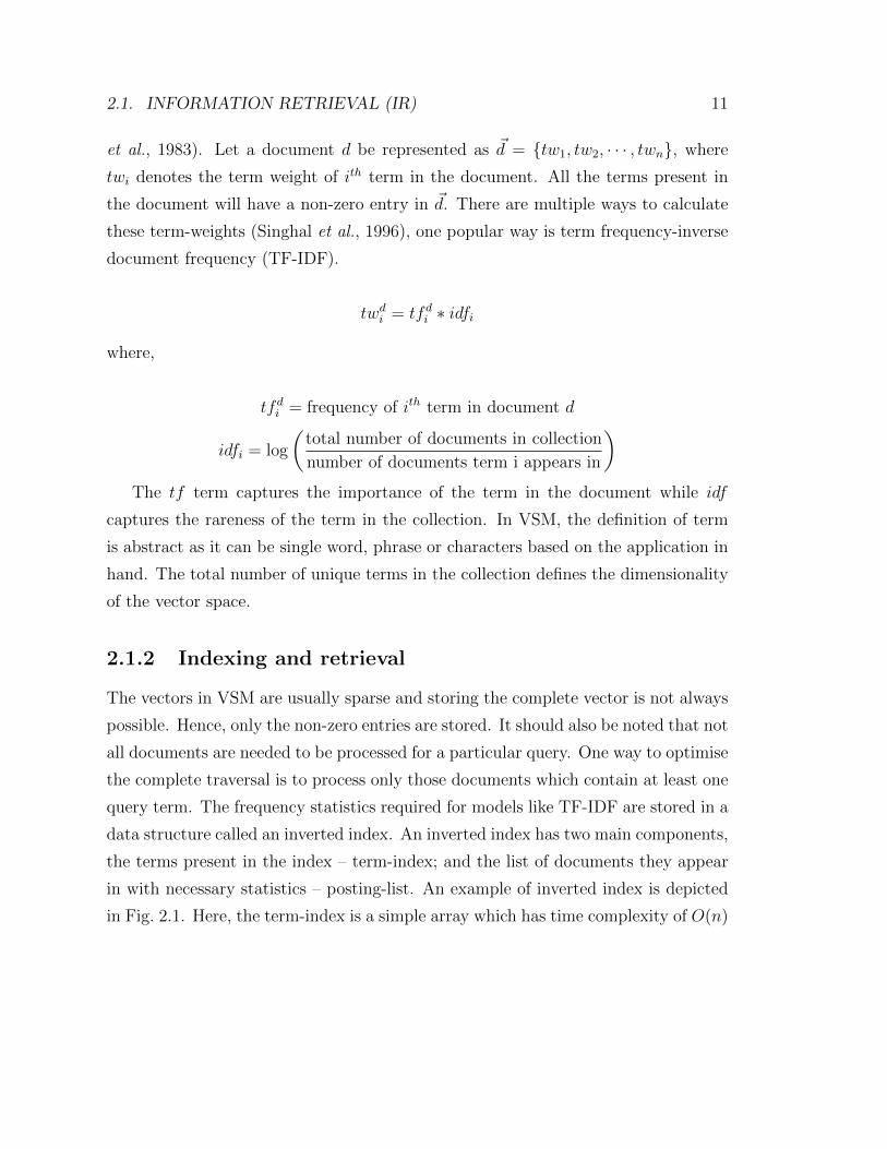
data structure called an inverted index. An inverted index has two main components,
the terms present in the index – term-index; and the list of documents they appear
in with necessary statistics – posting-list. An example of inverted index is depicted
in Fig. 2.1. Here, the term-index is a simple array which has time complexity of O(n)
12 CHAPTER 2. THEORETICAL BACKGROUND
term1
term2
termn
term3
term4
d2 5 d27 100
Term Index
Posting List
Figure 2.1: Inverted index. The example shows that term t1 is contained in documentsd2 and d27 with frequency 5 and 100 respectively.
while the posting-lists are storing the frequency of the terms in the corresponding
documents. There are many variants of the inverted index, mainly attributed by
their (search) time and space complexity constraints (Zobel and Moffat, 2006).
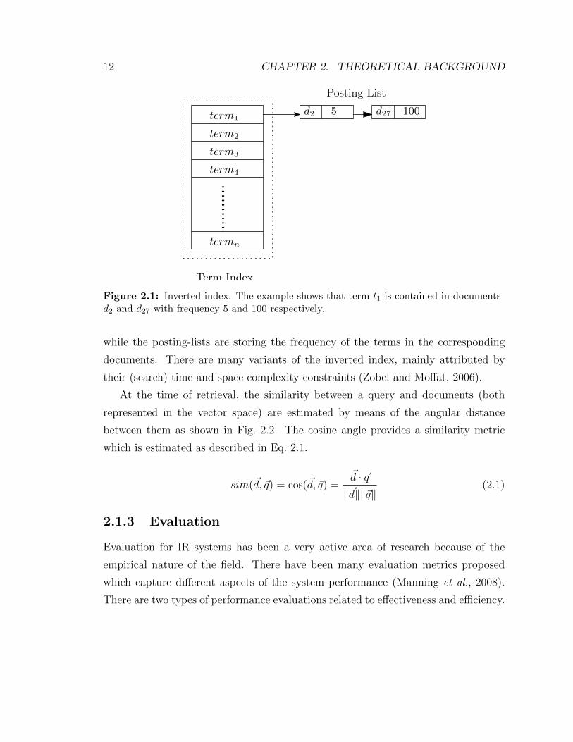
At the time of retrieval, the similarity between a query and documents (both
represented in the vector space) are estimated by means of the angular distance
between them as shown in Fig. 2.2. The cosine angle provides a similarity metric
which is estimated as described in Eq. 2.1.
sim(~d, ~q) = cos(~d, ~q) =~d · ~q‖~d‖‖~q‖
(2.1)
2.1.3 Evaluation
Evaluation for IR systems has been a very active area of research because of the
empirical nature of the field. There have been many evaluation metrics proposed
which capture different aspects of the system performance (Manning et al., 2008).
There are two types of performance evaluations related to effectiveness and efficiency.
2.1. INFORMATION RETRIEVAL (IR) 13
Figure 2.2: Documents and query represented in vector space.
The latter deals with the issues such as query latency and memory requirements.
While the former, the effectiveness, attracts larger research attention. It mainly
dwells around the concept of relevance. Although, relevance is a quite subjective
and abstract concept, it is usually captured by the manual relevance judgements
(qrels). Human judges are presented with a set of queries, document collection and
corresponding relevance judgements and they assign a binary label to the document:
relevant or non-relevant. The label relevant is assigned if the document satisfies the
information need expressed by the query.
Precision captures the ratio of the relevant documents among the retrieved doc-
uments and Recall captures the ratio of retrieved relevant documents among all the
relevant documents available in the collection. Most of the IR systems try to find a
trade-off between Precision and Recall with an extra bias towards either of them, de-
pending on the specific application. For example, web search engines are more keen
on Precision, while medicine or legal aspects related system care more for Recall.
Fβ-measure is a popular way of combining Precision and Recall, where β decides the
bias towards precision or recall. F1 gives equal weight to precision and recall while
F2 gives higher weight to recall and F0.5 gives higher weight to precision.
14 CHAPTER 2. THEORETICAL BACKGROUND
Fβ = (1 + β2) · precision× recall
(β2 · precision) + recall(2.2)
Average precision (AP) calculates precision at every recall point. AP provides a
way to estimate the quality of the ranklist. Sometimes, the relevance is labeled in
higher levels (graded-levels) to quantify better than binary. As the discussed metrics
so far work with binary relevance, we have used normalised discounted cumulative
gain (NDCG) which uses graded relevance as a measure of the usefulness, or gain,
from examining a document (Jarvelin and Kekalainen, 2002). Gain is calculated at
each ranking position and accumulated over all positions with a discount element.
The assumption is the relevant documents at lower position are less useful because
they are quite likely will not be examined by the user. A typical discount function
is 1log2(rank)
. The cumulative gain cgm for a ranklist of size m is calculated as:
cgm =m∑i=1
rel(di) (2.3)
where, rel(di) is graded-relevance of document di. Adding the discount term, dis-
counted cumulative gain dcgm becomes:
dcgm = rel(d1) +m∑i=2
rel(di)
log2(i)(2.4)
dcgm is normalised by the ideal ranklist upto m positions referred as idcgm to obtain
ndcgm.
ndcgm =dcgmidcgm
(2.5)
2.1.4 Semantic term-relatedness
Vector space models provide a way to compare documents and queries by means of
keyword matching. However, such lexical matching can be inaccurate due to the
fact that the relevance is often expressed by different vocabularies in documents and
2.2. DIMENSIONALITY REDUCTION 15
queries. One of the major hurdles in comparing text in VSM is to deal with problems
like synonymy and polysemy. Usually, in vector space, the documents are composed
of thousands of dimensions resulting in many meaningful associations between terms
being shadowed by large dimensions. There are models which try to handle this
problem in the vector space e.g. pseudo relevance feedback (PRF) (Rocchio, 1971;
Manning et al., 2008) and explicit semantic analysis (ESA) (Xu and Croft, 1996;
Gabrilovich and Markovitch, 2007; Anderka and Stein, 2009). PRF obtains top m
terms from top n documents and adds them to the original query and the expanded
query is used for the retrieval. ESA based approaches leverage on an external collec-
tion, such as Wikipedia, which is referred to as knowledge base. In ESA each word is
represented in the retrieval collection by its corresponding vector of document scores
in the knowledge base. Then, relatedness between two terms is calculated by the
cosine similarity between the corresponding vectors. Word sense disambiguation for
information retrieval has also been an active area of research (Sanderson, 1994; Liu
et al., 2005).
2.2 Dimensionality reduction
A formal definition of dimensionality reduction as per Burges (2010) is given as:
“Dimensionality reduction is the mapping of data to a lower dimensional space
such that uninformative variance in the data is discarded, or such that a subspace
in which the data lives is detected.”
Basically, it is a process of reducing the number of variables under consideration.
Dimensionality reduction techniques are widely popular in learning representation
of data in different modalities such as text, image, audio, video, etc (Fodor, 2002;
Burges, 2010). In this work we would focus concretely on approaches related to text
data.
Dimensionality reduction techniques can be achieved in two ways: (i) feature
selection; and (ii) feature extraction. The feature selection methods reduces the di-
16 CHAPTER 2. THEORETICAL BACKGROUND
mensionality by selecting a subset of features from the set of original features. The
feature selection methods of type filter , as defined in Guyon and Elisseeff (2003),
computes the score of each feature as a preprocessing step and the subset of features
are selected based on the scores assigned. In contrast to filter methods, wrapper
methods use the learning algorithms to assign scores to the features. Feature se-
lection techniques are widely used in machine learning based approaches, such as
classification (Dash and Liu, 1997; Yang and Pedersen, 1997; Janecek et al., 2008)
and ranking (Geng et al., 2007; Gupta and Rosso, 2012a).
On the other hand, the goal of the feature extraction based techniques is to
transform high dimensional data (Rn) into a much lower dimension representation
(Rm) pertaining the inherent structure of the original data where m << n. Such
low-dimensional space is commonly referred to as abstract space or latent space.
One such widely used approach is latent semantic indexing (LSI), which extracts
a low rank approximation of text data by means of singular value decomposition
(SVD) (Deerwester et al., 1990).
Dimensionality reduction techniques can broadly be categorised in two classes:
linear and non-linear. Usually, non-linear techniques can find more compact repres-
entations of the data compared to their linear counterparts (Hinton and Salakhutdinov,
2006). If there exists statistical dependence among the principal components of PCA,
or principal components have non-linear dependencies, PCA would require a larger
dimensionality to properly represent the data when compared to non-linear tech-
niques.
On the other hand, although non-linear projection methods such as multidimen-
sional scaling (MDS) give a way to obtain much better representations for mono
and cross-language similarity estimation; it is a transductive method (Cox and Cox,
2000; Banchs and Kaltenbrunner, 2008). It means MDS does not provide an operator
to project the unseen data into the target low dimensional space like the resulting
projection matrix in the case of PCA.
Latent semantic models such as LSI are able to correspond queries and relev-
2.2. DIMENSIONALITY REDUCTION 17
ant documents at the semantic level where lexical matching often fails (Deerwester
et al., 1990; Blei et al., 2003; Salakhutdinov and Hinton, 2009b,a; Platt et al., 2010;
Huang et al., 2013). These latent semantic models represent the text in a dense
low-dimensional semantic space, where semantically similar text fragments would be
closer to each other despite the fragments do not share any term. The semantic
representation is learned through the patterns of terms co-occurring in similar con-
texts. LSI extracts a low rank Gaussian approximation of a document-term matrix2
by means of singular value decomposition (SVD) (Deerwester et al., 1990). More
advanced approaches like probabilistic latent semantic analysis (PLSA) and latent
dirichlet allocation (LDA) observe the distribution of latent topics for the given doc-
uments (Hofmann, 1999; Blei et al., 2003).
Lately, dimensionality reduction techniques based on deep learning have become
very popular, especially deep autoencoders (DA). Deep autoencoders can extract
highly useful and compact features from the structural information of the data. Deep
autoencoders have proven to be very effective in learning reduced space representa-
tions of the data for similarity estimation, i.e. similar documents tend to have similar
abstract representations (Hinton and Salakhutdinov, 2006; Salakhutdinov and Hin-
ton, 2009a). Deep-learning is inspired by biological studies, which state the brain has
a deep architecture. Despite their high suitability to the task, deep learning did not
find much audience because of convergence issues until Hinton and Salakhutdinov
(2006) gave a way to initialise the network parameters in a good region for finding
optimal solutions.
However, these models are trained to optimise an objective function which is
only loosely related to the evaluation metric of the retrieval task. To overcome this
limitation, a new family of latent semantic models have emerged that exploits the
clickthrough data for semantic modelling Gao et al. (2010, 2011); Huang et al. (2013).
These models take into account an explicit relevance signal in terms of the query and
2Such matrix is composed by the documents in the collection (rows) and all the unique termsin the collection (columns). Each entry in the matrix contains the weight of a particular term in adocument e.g. term frequency.
18 CHAPTER 2. THEORETICAL BACKGROUND
its clicked document.
2.3 IR across languages
Cross-language information retrieval (CLIR) is a special case of IR, where the query
and the documents are in different languages. Due to the existing needs in different
multi lingual scenarios, various CLIR applications became popular. Cross-language
ad-hoc retrieval, cross-language plagiarism detection and parallel/comparable text
discovery are examples of some popular and important problems.
In general, there are two ways to address the language mismatch between query
and documents: (i) translate either of them to the language of the other and perform
monolingual IR; and (ii) obtain a language agnostic translingual space where both
of them can be compared. The former takes the path of machine translation while
the latter falls under the dimensionality reduction techniques3.
The translation approaches try to normalise language mismatch between query
and documents using various resources such as bilingual dictionaries, multilingual
thesaurus, multilingual semantic network etc. Machine translation systems leverage
on a translation model (estimating segment-level4 translation probabilities) that is
combined with a target language model. The language model helps aligning the
potential segment-level translations to form a valid sentence. Typically, machine
translation based approaches for CLIR do not employ the full MT pipeline, instead
they exploit the translation probabilities to formulate the translated query (Gao
et al., 2001; Ture and Lin, 2014). Moreover, the MT based approaches often employ
lexical, syntactic and semantic linguistic analysis. Though such pipeline ensures the
representation is rich, they are mainly deviced for the MT task and this representa-
tion may not be that helpful for the retrieval task.
Though the MT based language normalisation can be highly accurate, the re-
3Though one can use dimensionality reduction techniques on machine translated text, what werefer here is to obtain translingual representation using dimensionality reduction techniques.
4Including both single words and multi-word phrases.
2.3. IR ACROSS LANGUAGES 19
trieval suffers from the issues of VSM such as sparsity, synonymy and polysemy.
Moreover, MT can be very slow, limiting its use on large training datasets (Platt
et al., 2010; Gupta et al., 2016b). Alternatively, the cross-language latent semantic
models provide a way to model cross-language term associations in a latent space.
Such models include LSA based cross-language latent semantic analysis (CL-LSA) (Du-
mais et al., 1997), in which a cross-language document-term matrix is constructed by
concatenating the parallel data. Canonical correlation analysis (CCA) based meth-
ods find projections that maximise the correlation between the projected vectors of
parallel data (Vinokourov et al., 2002). Generative models, such as LDA, are used
to represent bilingual data into hidden topical space (Mimno et al., 2009). Ori-
ented principal component analysis (OPCA) introduces the noise covariance matrix
and solves the generalised eigenvalue problem (Diamantaras and Kung, 1996; Platt
et al., 2010). Deep bilingual autoencoders (BAE) are used to represent bilingual
data in a low-dimensional joint space by optimising the reconstruction error (Lauly
et al., 2014; Chandar A. P. et al., 2014; Gupta et al., 2014). Siamese neural network
based S2Net learns discriminatively the projection matrix from the pairs of related
and unrelated documents (Yih et al., 2011). Except for the S2Net method, all these
models derive cross-language representations in an unsupervised manner by optim-
ising an objective function that is only loosely related to the evaluation metric for
the retrieval task. Some of these models are reviewed in detail in Chapter 6. Another
family of models for cross-language natural language processing applications require
advanced syntactic information in the input, such as syntactic parse trees (Socher
et al., 2012; Hermann and Blunsom, 2013). Similar models sometimes also require
word-alignments during the training (Klementiev et al., 2012; Zou et al., 2013; Miko-
lov et al., 2013). Such requirements limit the use of these approaches to resource
fortunate languages.
20 CHAPTER 2. THEORETICAL BACKGROUND
2.4 IR across scripts
Although IR across scripts, which is referred to as mixed-script IR, has attained very
little attention explicitly, many tangentially related problems like CLIR and trans-
literation for IR discuss some of the issues of MSIR. While languages like Chinese
and Japanese use multiple scripts (Qu et al., 2003), they may not illustrate the true
complexity of the MSIR scenario described here because there are standard rules and
preferences for script usage and well defined spellings rules. In Roman translitera-
tion of Hindi, on the other hand, there are no standard rules, which leads to a large
number of spelling variations for a single term. Furthermore, these texts are often
mixed with English, which makes detection of transliterated text quite difficult.
CLIR typically involve translating queries from one language to another. How-
ever, it is often a reasonable choice to transliterate certain OOV words, especially
NEs. There has been a large body of work that specifically targets the problem of
named entity transliteration in CLIR.
However, training and testing transliteration systems requires data and, for Names
Entities, data creation has been typically through mining text corpora. Shared tasks
such as those conducted by NEWS5 and FIRE6 have also been successful to an extent
in both data sharing and bench-marking various machine transliteration techniques
and systems.
In an analysis of the query logs for Greek web users, Efthimiadis et al. (2009) have
shown that 90 percent of the queries are formulated using the Roman alphabet while
only 8% use the Greek alphabet, and the reason for this (Efthimiadis, 2008) is that 1
in 3 Greek navigational queries fail due to the low level of indexing of the Greek web.
Wang et al. (2008) employ a translation based method to classify non-English queries
using an English taxonomy system. Though their method shows some promise,
it is heavily dependent on the availability of translation systems for the language
pairs in question. Ahmed et al. (2011) show that the problem of transliteration is
5http://translit.i2r.a-star.edu.sg/news2012/6http://www.isical.ac.in/ fire/
2.4. IR ACROSS SCRIPTS 21
further challenging because of the fact that due to a lack of standardization in the
way a local language is mapped to the Roman script, there is a large variation in
spellings. In their work on query-suggestion for a Bollywood Song Search system Dua
et al. (2011) also stress on the presence of valid variations in spelling Hindi words
in Roman script. Related work by Gupta et al. (2012a) goes into the details of
handling these variations while mining transliterated pairs from Bollywood song
lyric data. Edit-distance based approaches have also been popular for the generation
of such pairs; such as, for instance, English-Telugu (Sowmya and Varma, 2009) and
Tamil-English (Janarthanam et al., 2008). Pal et al. (2008) propose a method for
normalization of transliterated text that combines two techniques: (i) a stemmer
based method that deletes commonly used suffixes (Oard et al., 2001) with rules for
mapping variants to a single canonical form; (ii) a similar method that uses both
stemming and grapheme-to-phoneme conversion is used by Raj and Maganti (2009)
to develop a proof-of-concept for a multilingual search engine that supports 10 Indian
languages. Thus, though there has been some interest in the past, especially with
respect to handling variation and normalization of transliterated text, the challenge
of IR in the mixed-script space is largely neglected.
For languages like Japanese, Chinese, Arabic and most Indian languages, the
challenge of text input in native script has resulted in a proliferation of translit-
erated documents on the web. While the availability of more sophisticated and
user-friendly input methods have helped resolving this for some of these languages
(for example Japanese and Chinese), there is still a large number of languages for
which the English keyboard (and hence the Roman script) remains the main input
medium. Further, as a number of relevant documents are available in both the nat-
ive script and its transliterated form, it also becomes important to deal with not
only cross-language but mixed-script IR for such languages. Social media is another
domain where the use of transliterated text is widespread. Here, text normalization
is complicated further by the presence of SMS-like contractions, interjections and
code-mixing (the switching between languages at phrase, word and morphological
22 CHAPTER 2. THEORETICAL BACKGROUND
levels). As IR becomes more pervasive in social media, dealing with the complexities
of transliteration will become more significant for a robust search engine.
2.5 Cross-view models
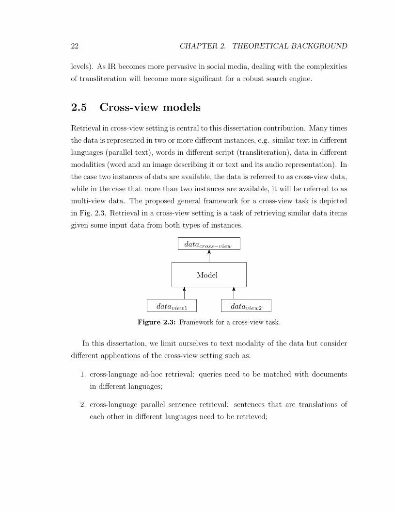
Retrieval in cross-view setting is central to this dissertation contribution. Many times
the data is represented in two or more different instances, e.g. similar text in different
languages (parallel text), words in different script (transliteration), data in different
modalities (word and an image describing it or text and its audio representation). In
the case two instances of data are available, the data is referred to as cross-view data,
while in the case that more than two instances are available, it will be referred to as
multi-view data. The proposed general framework for a cross-view task is depicted
in Fig. 2.3. Retrieval in a cross-view setting is a task of retrieving similar data items
given some input data from both types of instances.
dataview1 dataview2
Model
datacross−view
Figure 2.3: Framework for a cross-view task.
In this dissertation, we limit ourselves to text modality of the data but consider
different applications of the cross-view setting such as:
1. cross-language ad-hoc retrieval: queries need to be matched with documents
in different languages;
2. cross-language parallel sentence retrieval: sentences that are translations of
each other in different languages need to be retrieved;
2.5. CROSS-VIEW MODELS 23
3. cross-language plagiarism detection: plagiarised sections from the suspicious
documents need to be identified from source documents in different languages;
4. mixed-script IR: queries need to be matched with documents written in the
same language but different scripts.
The detailed description of these tasks and experimental framework are presented
in Chapters 6 and 5.

Chapter 3Neural networks background
This chapter covers the technical background needed to understand the proposed
models in the thesis. First, we will provide an introduction to neural networks and
restricted Boltzmann machines followed by autoencoders. We will also review the
backpropagation algorithm and few relevant optimisation techniques.
3.1 Neural networks
Neural networks or artificial neural networks are a family of models inspired by
biological neural networks. These models are used to approximate complex unknown
functions that usually depend on a large number of inputs. The fundamental unit of
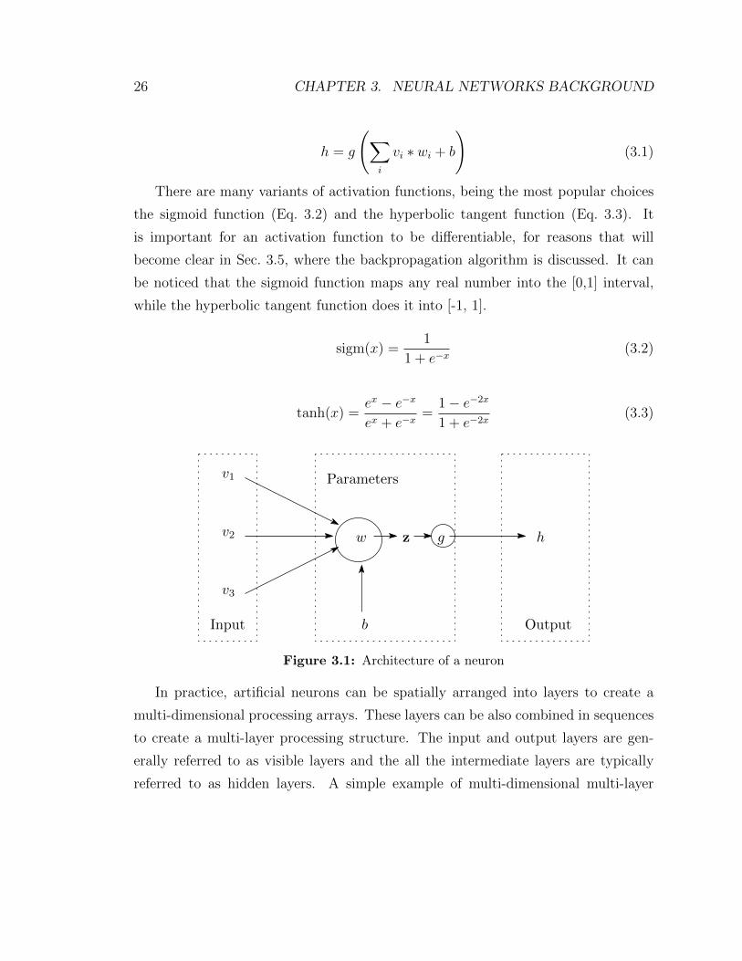
a neural network is the artificial neuron. Fig. 3.1 shows the architecture of a single
artificial neuron with input vector v ∈ Rn, output h ∈ Rm and a parameter set of
weights w and bias b. Such basic processing unit, which is called an artificial neuron,
encodes the input information into a real number output h, as shown in Eq. 3.1;
where g is a non-linear activation function.
25
26 CHAPTER 3. NEURAL NETWORKS BACKGROUND
h = g
(∑i
vi ∗ wi + b
)(3.1)
There are many variants of activation functions, being the most popular choices
the sigmoid function (Eq. 3.2) and the hyperbolic tangent function (Eq. 3.3). It
is important for an activation function to be differentiable, for reasons that will
become clear in Sec. 3.5, where the backpropagation algorithm is discussed. It can
be noticed that the sigmoid function maps any real number into the [0,1] interval,
while the hyperbolic tangent function does it into [-1, 1].
sigm(x) =1
1 + e−x(3.2)
tanh(x) =ex − e−xex + e−x
=1− e−2x
1 + e−2x(3.3)
b
v1
v2
v3
h
OutputInput
Parameters
w gz
Figure 3.1: Architecture of a neuron
In practice, artificial neurons can be spatially arranged into layers to create a
multi-dimensional processing arrays. These layers can be also combined in sequences
to create a multi-layer processing structure. The input and output layers are gen-
erally referred to as visible layers and the all the intermediate layers are typically
referred to as hidden layers. A simple example of multi-dimensional multi-layer
3.1. NEURAL NETWORKS 27
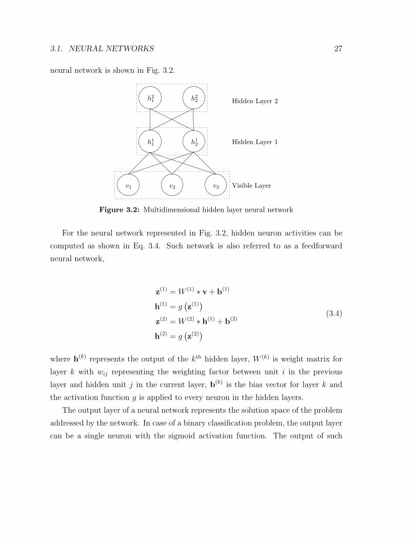
neural network is shown in Fig. 3.2.
v1 v2 v3
h11 h1
2
h21 h2
2
Visible Layer
Hidden Layer 1
Hidden Layer 2
Figure 3.2: Multidimensional hidden layer neural network
For the neural network represented in Fig. 3.2, hidden neuron activities can be
computed as shown in Eq. 3.4. Such network is also referred to as a feedforward
neural network,
z(1) = W (1) ∗ v + b(1)
h(1) = g(z(1))
z(2) = W (2) ∗ h(1) + b(2)
h(2) = g(z(2))
(3.4)
where h(k) represents the output of the kth hidden layer, W (k) is weight matrix for
layer k with wij representing the weighting factor between unit i in the previous
layer and hidden unit j in the current layer, b(k) is the bias vector for layer k and
the activation function g is applied to every neuron in the hidden layers.
The output layer of a neural network represents the solution space of the problem
addressed by the network. In case of a binary classification problem, the output layer
can be a single neuron with the sigmoid activation function. The output of such
28 CHAPTER 3. NEURAL NETWORKS BACKGROUND
neuron can be interpreted as the probability p for the corresponding input datapoint
to belong to a certain class and (1 − p) as the probability to not belong. In case
of a multi-class classification problem, the output layer is usually of size equal to
the number of classes and, often, the softmax normalization function is applied at
output layer. The softmax function allows the output layer of the network to model
a probability distribution in which each neuron represents the probability of one of
the considered classes. The softmax normalization function is shown in Eq. 3.5. For
non-classification tasks such as regression, representation learning or projection, the
output layer represents a multi-dimensional continuous space in which the input data
is projected.
softmax(hj) =ehj∑Kk=1 e
hk, for j = 1, 2, .., K (3.5)
3.2 Restricted Boltzmann machines (RBM)
Restricted Boltzmann machines have been used as generative models for many dif-
ferent types of data including images (Hinton and Salakhutdinov, 2006), speech (Mo-
hamed et al., 2012), documents (Salakhutdinov and Hinton, 2009b), and user rat-
ings (Salakhutdinov et al., 2007). A restricted Boltzmann machine is a two-layer
bipartite network with a visible layer (v) and a hidden layer (h). Both layers are
connected through symmetric weights (w). In this kind of models the hidden units
play the role of latent variables. Depending on the type of input data, two different
variants of the visible layer can be selected: binary or multinomial. In case of binary
RBM the visible layer is stochastic binary layer which accepts data in binary form.
While, in case of multinomial RBM, visible layer is multinomial to accept data which
follows multinomial distribution. The multinomial RBM is based on the replicated
softmax model (RSM) (Salakhutdinov and Hinton, 2009b). Following, we present
more details on the two RBM.
3.2. RESTRICTED BOLTZMANN MACHINES (RBM) 29
3.2.1 Stochastic binary RBM
In a stochastic binary RBMs both, visible and hidden, layers are stochastic binary
units with sigmoid non-linearity. Let visible units v ∈ {0, 1}n be binary input vari-
ables and hidden units h ∈ {0, 1}m be hidden latent variables. Energy-based models
have an energy value associated to each configuration of the variables (i.e., paramet-
ers) of of the model. Parameters updated through the learning algorithm modify this
energy and usually, the desirable parameters have low energy. RBMs are commonly
explained using energy-based models (LeCun et al., 2006). The energy of the state
{v,h} is defined as follows:
E(v,h) = −n∑i=1
aivi −m∑j=1
bjhj −∑i,j
vihjwij (3.6)
where vi, hj are the binary states of visible unit i and hidden unit j, ai, bj are their
biases and wij is the weight between them.
Then, it is possible to obtain visible and hidden activities in both directions as
shown below,
p(vi = 1|h) = g(ai +∑j
hjwij) (3.7)
p(hj = 1|v) = g(bj +∑i
viwij) (3.8)
where g(x) = 1/(1 + exp(−x)) is the logistic sigmoid function.
3.2.2 Multinomial RBM
The multinomial RBM is based on the Replicated Softmax model proposed by
Salakhutdinov and Hinton (2009b).
Let v ∈ {1, . . . , K}n, where K is the number of trials parameter of multinomial
distribution, n is the input dimensionality and let h ∈ {0, 1}m be stochastic binary
hidden latent variables. Considering an input with K trials, the energy of the state
30 CHAPTER 3. NEURAL NETWORKS BACKGROUND
{v,h} is defined as:
E(v,h) = −n∑i=1
vkak −Dm∑j=1
bjhj −∑k,j
wkijhj vk (3.9)
where vki denotes the count (k) data for the ith term.
In the RSM, the visible layer implements a softmax normalizing function. The
resulting multinomial visible units represent the probability distribution of the word-
counts. In multinomial RBM, the visible and hidden units are updated as shown
below,
p(vki = 1|h) =exp(bki +
∑j hjW
kij)∑K
q=1 exp(bqi +∑
j hjWqij)
(3.10)
p(hj = 1|V) = σ(aj +D∑i=1
K∑k=1
vkiWkij) (3.11)
3.3 Text representation
Text can be represented in vector form, popularly referred as bag-of-words. All
possible words from the corpus constitute a vocabulary of unique words. These
words in vocabulary form a high-dimensional vector space where each word refers
to a dimension. A text can be represented as either a binary vector where non-zero
dimension denotes existance of that word in the text or a count vector where non-
zero dimension denotes the count of that word in the text. It is a common practice
to remove stopwords from the vocabulary and apply stemming.
3.4. AUTOENCODER 31
3.4 Autoencoder
The autoencoder is a neural network architecture that approximates the identity
function by replicating its input as its output. The input and output dimensions of
the network are the same (n). The autoencoder approximates the identity function
in two steps: (i) coding (reduction); and (ii) decoding (reconstruction). The coding
step maps the input x ∈ Rn into an intermediate representation y ∈ Rm where
m < n. The mapping can be seen as a function y = g(x) with g : Rn → Rm. On
the other hand, the decoding step maps the intermediate representation y into the
output x ∈ Rn in such a way that x ≈ x. The decoding step can be seen as a
function x = f(y) with f : Rm → Rn. The two-step autoencoder can be seen as
the composition of an encoding function g(x) and a decoding function f(x), which
approximates the identity function: f(g(x)) ≈ x using reconstruction error:
reconstruction error =1
2||f(g(x))− x||2 (3.12)
In an autoencoder, the visible layer corresponds to the input x and the hidden
layer corresponds to the intermediate representation y. Autoencoders can have a
single hidden layer or multiple hidden layers. If there is only one single hidden layer,
the optimal solution remains the PCA projection (Bourlard and Kamp, 1988). In
order to overcome some of the PCA limitations, a common practice is to stack mul-
tiple RBMs, constituting what is called a deep architecture. Those deep architectures
have been proven to produce highly non-linear and powerful reduced space repres-
entation (Hinton and Salakhutdinov, 2006). Autoencoders made up from multiple
RBMs are referred to as deep autoencoders. Both of the considered models differ
in the way they model the text data. While the binary deep autoencoder (bDA)
models the presence of the term into the document (binary), the multinomial deep
autoencoder (rsDA) directly models the count of the term (i.e., term frequency) in
the document. An example of deep architecture is shown in Fig. 3.3.
32 CHAPTER 3. NEURAL NETWORKS BACKGROUND
3.5 Backpropagation
Backpropagation is an efficient method to train a multi-layered feedforward neural
network (Rumelhart et al., 1986). It is typically used in conjunction with an optim-
isation method, such as gradient descent, which is discussed in more detail in Sec. 3.6.
In backpropagation the gradient of a loss function is calculated with respect to the
network parameters: weights and biases. The information of the gradient is recurs-
ively used to update the parameters in such a way that the specified loss function is
reduced at each iteration step. Backpropagation is a supervised method because it
needs to know the correct output in order to compute the loss function. An important
condition for the use of backpropagation is that all transfer functions at each layer
should be differentiable, otherwise the gradient calculation is not possible. Both, the
errors calculated at the output layer and the corresponding gradient are propagated
backwards through the entire network, hence the name of “backpropagation”.
An important step in neural network training is the definition of the loss function
J(θ), where θ represents the set of network parameters. One popular choice for loss
function is the mean squared error (MSE), which is defined as J(θ) = 12(y − h)2,
where y is label and h is neural network output. Using the terminology introduced
in Fig. 3.1 and considering a neural network with 2-hidden layers with sigmoid activ-
ation function and one single output, the gradient computation at the output layer
is shown in Eq. 3.13.
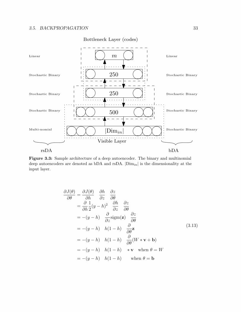
3.5. BACKPROPAGATION 33
|Dimin|
500
250
m
Visible Layer
Bottleneck Layer (codes)
250
Stochastic Binary
Stochastic Binary
Stochastic Binary
Stochastic Binary
Linear
Multi-nomial
Stochastic Binary
Stochastic Binary
Stochastic Binary
Linear
rsDA bDA
Figure 3.3: Sample architecture of a deep autoencoder. The binary and multinomialdeep autoencoders are denoted as bDA and rsDA. |Dimin| is the dimensionality at theinput layer.
∂J(θ)
∂θ=∂J(θ)
∂h
∂h
∂z
∂z
∂θ
=∂
∂h
1
2(y − h)2 ∂h
∂z
∂z
∂θ
= −(y − h)∂
∂zsigm(z)
∂z
∂θ
= −(y − h) h(1− h)∂
∂θz
= −(y − h) h(1− h)∂
∂θ(W ∗ v + b)
= −(y − h) h(1− h) ∗ v when θ = W
= −(y − h) h(1− h) when θ = b
(3.13)
34 CHAPTER 3. NEURAL NETWORKS BACKGROUND
These gradients for parameters W and b can be backpropagated to the previous
layers by using the chain rule. As shown in Eq. 3.14, the gradient at the lth layer
can be computed in terms of the already known gradient of the (l + 1)th layer.
δl =∂J(θ)
∂θl
=∂J(θ)
∂zl+1
∂zl+1
∂zl
∂zl∂θl
= δl+1∂zl+1
∂hl
∂hl∂zl
∂zl∂θl
= δl+1∂
∂al(Wl+1 ∗ hl + bl+1)
∂hl∂zl
∂zl∂θl
= δl+1 ∗ Wl+1 h(1− h)∂zl∂θl
(3.14)
3.6 Optimisation
Neural network parameters can be updated using an optimisation method called
gradient descent. Gradient methods are first-order optimisation algorithms that
converge towards a local optimum of an objective function by taking consecutive
steps that are proportional to the gradient. If the algorithm moves towards local
minima using steps that are proportional to the negative gradient, it is called gradient
descent; and if it moves towards local maxima using steps that are proportional to
positive gradient, it is called gradient ascent. Under gradient descent, parameters of
a model at iteration t are updated as shown in Eq. 3.15:
θ(t+1) = θ(t) − αδ(t) (3.15)
where α is learning rate and δ denotes gradient.
Usually the gradients are accumulated over all the datapoints (m) of the training
set and the weights are updated as shown in Eq. 3.16:
3.6. OPTIMISATION 35
θ(t+1)w = θ(t)
w − αm∑i=1
(−(yi − ai) · ai · (1− ai) ∗ vi) (3.16)
In practice, sometimes it is not possible to compute the sum of the gradient
over all the datapoints in one pass before update due to computational issues, such
as gradient might overflow, hence the updates are made at each datapoint. It is a
common practice, when using gradient descent, that the dataset is randomly shuffled
to avoid possible bias towards specific regions of the objective function. Then the
updates are made as shown in Algorithm 1. This process is called stochastic gradient
descent.
Algorithm 1: Stochastic gradient descent.
1 initialise θ randomly;
2 shuffle training data randomly;
3 for each training data point i ∈ m do
4 θ(i) = θ(i) − αδ(i)
It is often shown that advanced optimisation methods such as conjugate gradi-
ent (Hestenes and Stiefel, 1952) or L-BFGS (Nocedal, 1980) are faster and are able
to exhibit better convergence. Another common practice is to update the model
parameters with gradients accumulated over a small batch of datapoints, instead of
updating the model parameters after each datapoint or all datapoins. Such batches
are called mini-batches. This kind of updates are also computationally efficient be-
cause they can better use multiple cores of CPUs or GPUs.

Chapter 4Cross-view models
This chapter aims at describing the main contributions of this thesis . Retrieval
across different continuous space representations is central to the thesis contributions
as described in Chapter 2. In recent years there is a surge and rapid growth in the
neural network community around deep neural networks and deep learning. Data
availability has grown large. This, along with a new break-through in computing re-
search and especially in graphical processing units (GPUs), has allowed for often com-
putationally expensive tasks such as training deep neural networks to become feasible
from the experimental point of view. Most of the current research in deep learning is
focused on single-embedding applications in different languages. This thesis focuses
on the use of deep neural models for cross-embedding applications; more specifically
two different cases are considered: cross-language and cross-script. In this chapter,
we describe two novel techniques to capture similarities across different embeddings
to aid cross-embedding retrieval: (i) cross-view autoencoder for mixed-script IR,
and (ii) external data composition neural networks (XCNN) for cross-language IR.
The cross-view autoencoder uses the RBM pretraining to initialise the network and
37
38 CHAPTER 4. CROSS-VIEW MODELS
then, the network is tuned using the autoencoder backpropagation. This architec-
ture has shown promise in uncovering the meaningful representations (Hinton and
Salakhutdinov, 2006). Hence, we take that architecture to cross-view setting, es-
pecially at character-level, to model mixed-script terms. On the other hand, there
has been significant progress in terms of learning word-embeddings and representing
text through composition (Mikolov et al., 2013; Hermann and Blunsom, 2014). In
XCNN, we learn bilingual word-embeddings through composition neural networks
addressing some of the limitations of the present models.
4.1 Cross-view autoencoder (CAE) for mixed-script
IR
As discussed in Chapters 2 and 5, the primary challenge in mixed-script retrieval
is to model and match terms across both scripts and spelling variations, which are
especially common in the non-native scripts. We shall refer to the variants of the
same word in the native and other scripts as term equivalent. The term matching
problem can be addressed by using existing approaches such as approximate string
matching (Hall and Dowling, 1980; Zobel and Dart, 1996) and transliteration min-
ing (Udupa and Khapra, 2010a; Kumaran et al., 2010; Kumar and Udupa, 2011).
The former is especially useful to handle spelling variations in a single script, while
the latter can help in matching terms across the scripts. However, these methods
cannot be directly used for term matching over a single and across multiple scripts
at the same time.
In this section, we propose a framework for jointly modelling terms across scripts.
We achieve this by learning a low-dimensional representation of terms in a common
abstract space where term equivalents are close to each other. The concept of com-
mon abstract space for term equivalents is based on the fundamental observation
that words are transliterated into a non-native script in such a way that its sound
or pronunciation is preserved. Thus, if we can represent the pronunciation of words
4.1. CROSS-VIEW AUTOENCODER (CAE) FOR MIXED-SCRIPT IR 39
in an abstract space, it could faithfully embed terms written in any script in such a
way that term equivalents are close to each other as far as they have similar pronun-
ciations.1
4.1.1 Formulation
In order to build the intended models, we treat the phonemes as character-level “top-
ics” within the terms. There is a good number of examples of word-level topic models
using undirected graphical models like restricted Boltzmann machines (Gehler et al.,
2006; Salakhutdinov and Hinton, 2009a,b). These models are usually based on the
assumption that each document is represented as a mixture of topics, where each
topic defines a probability distribution over words. Similarly, in our proposed model,
we consider the terms to be represented as a mixture of “topics”, where each topic
defines a probability distribution over character n-grams.
Phonemes can be captured by character n-grams. Consider the feature set F =
{f1, . . . , fK} containing character grams of scripts si for all i ∈ {1, ., r} and |F| = K.
Let t1 =⋃i=1...r w1,i be a datum from training data T of language l1, where w1,i
represents a word w written in language l1 and script si, and r is the number of
scripts being modelled jointly. The datum can be represented as K-dimensional
feature vector x where xk is the count of kth feature fk ∈ F in datum t1.
We assume that count of character grams within terms follow a Dirichlet-multinomial
distribution. Consider N independent draws from a categorical distribution with K
categories. In the present context, N =∑K
i xi and {f1, . . . , fK} are K categories,
where the number of times a particular feature fk occurs in the datum t1 is denoted
as xk. Then x = (x1, . . . , xK) follows a multinomial distribution with parameters
N and p, where p = (p1, . . . , pK) and pk is the probability that kth feature takes
1Not all scripts are used to represent the words according to their basic sounds or phonemes.For example, the Chinese script is a notable exception. However, most of the scripts (includingRoman, Cyrillic, Arabic, Indic and other South Asian scripts) are more or less based on a phonemicorthography where words are broken down into syllables or phonemes and represented using letters.Hence, our method is applicable to these scripts.
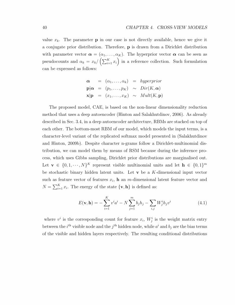
40 CHAPTER 4. CROSS-VIEW MODELS
value xk. The parameter p in our case is not directly available, hence we give it
a conjugate prior distribution. Therefore, p is drawn from a Dirichlet distribution
with parameter vector α = (α1, . . . , αK). The hyperprior vector α can be seen as
pseudocounts and αk = xk/(∑K
i=1 xi
)in a reference collection. Such formulation
can be expressed as follows:
α = (α1, . . . , αk) = hyperprior
p|α = (p1, . . . , pK) ∼ Dir(K,α)
x|p = (x1, . . . , xK) ∼ Mult(K,p)
The proposed model, CAE, is based on the non-linear dimensionality reduction
method that uses a deep autoencoder (Hinton and Salakhutdinov, 2006). As already
described in Sec. 3.4, in a deep autoencoder architecture, RBMs are stacked on top of
each other. The bottom-most RBM of our model, which models the input terms, is a
character-level variant of the replicated softmax model presented in (Salakhutdinov
and Hinton, 2009b). Despite character n-grams follow a Dirichlet-multinomial dis-
tribution, we can model them by means of RSM because during the inference pro-
cess, which uses Gibbs sampling, Dirichlet prior distributions are marginalised out.
Let v ∈ {0, 1, · · · , N}K represent visible multinomial units and let h ∈ {0, 1}mbe stochastic binary hidden latent units. Let v be a K-dimensional input vector
such as feature vector of features xi, h an m-dimensional latent feature vector and
N =∑K
i=1 xi. The energy of the state {v,h} is defined as:
E(v,h) = −K∑i=1
viai −Nm∑j=1
bjhj −∑i,j
W ijhjv
i (4.1)
where vi is the corresponding count for feature xi, Wij is the weight matrix entry
between the ith visible node and the jth hidden node, while ai and bj are the bias terms
of the visible and hidden layers respectively. The resulting conditional distributions
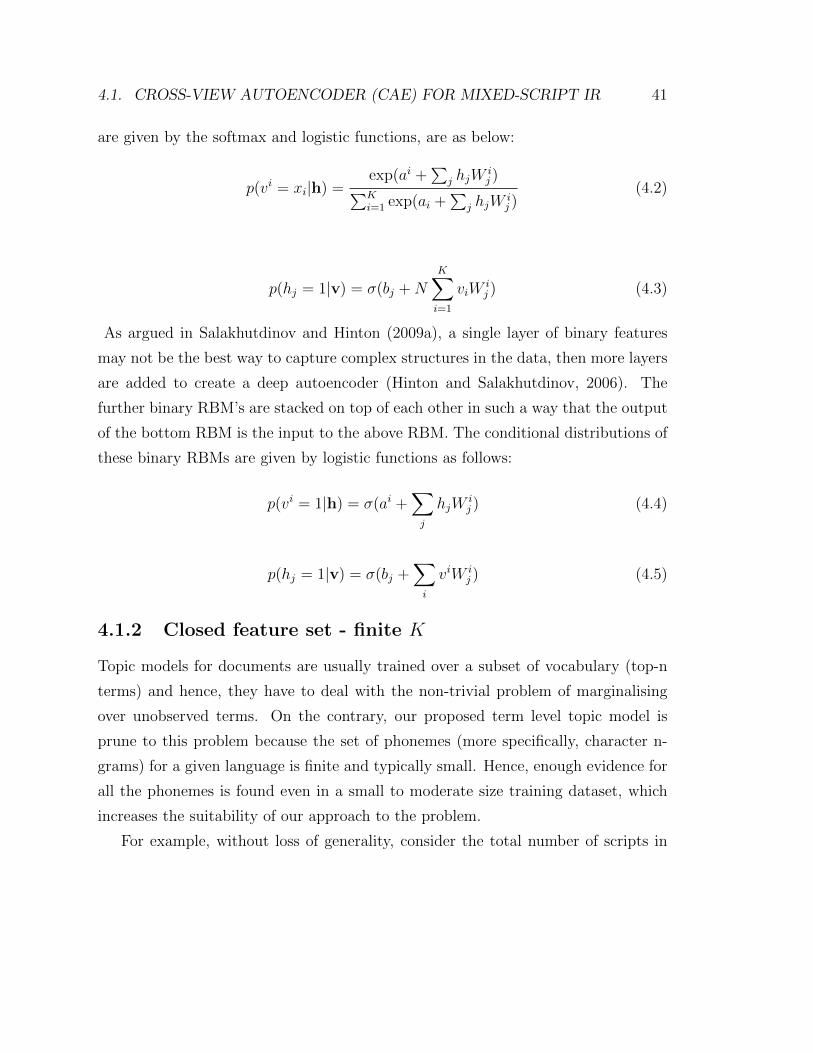
4.1. CROSS-VIEW AUTOENCODER (CAE) FOR MIXED-SCRIPT IR 41
are given by the softmax and logistic functions, are as below:
p(vi = xi|h) =exp(ai +
∑j hjW
ij )∑K
i=1 exp(ai +∑
j hjWij )
(4.2)
p(hj = 1|v) = σ(bj +NK∑i=1
viWij ) (4.3)
As argued in Salakhutdinov and Hinton (2009a), a single layer of binary features
may not be the best way to capture complex structures in the data, then more layers
are added to create a deep autoencoder (Hinton and Salakhutdinov, 2006). The
further binary RBM’s are stacked on top of each other in such a way that the output
of the bottom RBM is the input to the above RBM. The conditional distributions of
these binary RBMs are given by logistic functions as follows:
p(vi = 1|h) = σ(ai +∑j
hjWij ) (4.4)
p(hj = 1|v) = σ(bj +∑i
viW ij ) (4.5)
4.1.2 Closed feature set - finite K
Topic models for documents are usually trained over a subset of vocabulary (top-n
terms) and hence, they have to deal with the non-trivial problem of marginalising
over unobserved terms. On the contrary, our proposed term level topic model is
prune to this problem because the set of phonemes (more specifically, character n-
grams) for a given language is finite and typically small. Hence, enough evidence for
all the phonemes is found even in a small to moderate size training dataset, which
increases the suitability of our approach to the problem.
For example, without loss of generality, consider the total number of scripts in
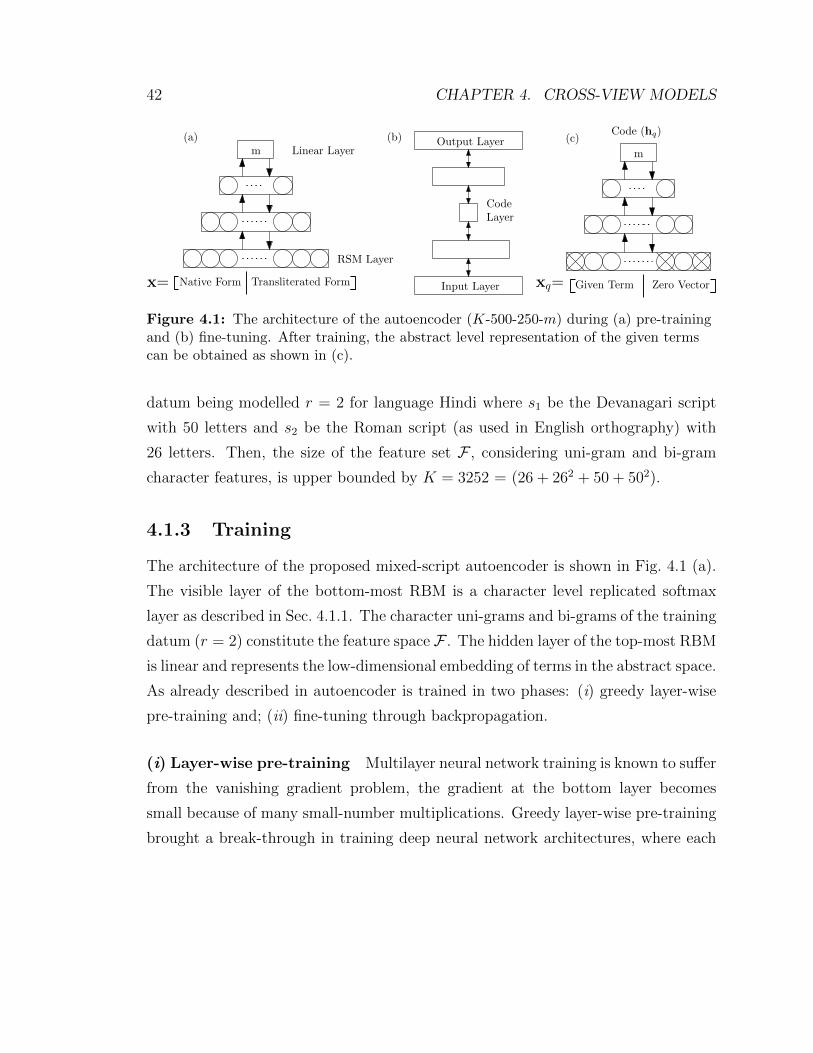
42 CHAPTER 4. CROSS-VIEW MODELS
m Linear Layer
RSM Layer
Transliterated Form
CodeLayer
Output Layer
Input Layer
(a) (b)
m
Given Term Zero Vector
Code (hq)
Native Form
(c)
x= xq=
Figure 4.1: The architecture of the autoencoder (K-500-250-m) during (a) pre-trainingand (b) fine-tuning. After training, the abstract level representation of the given termscan be obtained as shown in (c).
datum being modelled r = 2 for language Hindi where s1 be the Devanagari script
with 50 letters and s2 be the Roman script (as used in English orthography) with
26 letters. Then, the size of the feature set F , considering uni-gram and bi-gram
character features, is upper bounded by K = 3252 = (26 + 262 + 50 + 502).
4.1.3 Training
The architecture of the proposed mixed-script autoencoder is shown in Fig. 4.1 (a).
The visible layer of the bottom-most RBM is a character level replicated softmax
layer as described in Sec. 4.1.1. The character uni-grams and bi-grams of the training
datum (r = 2) constitute the feature space F . The hidden layer of the top-most RBM
is linear and represents the low-dimensional embedding of terms in the abstract space.
As already described in autoencoder is trained in two phases: (i) greedy layer-wise
pre-training and; (ii) fine-tuning through backpropagation.
(i) Layer-wise pre-training Multilayer neural network training is known to suffer
from the vanishing gradient problem, the gradient at the bottom layer becomes
small because of many small-number multiplications. Greedy layer-wise pre-training
brought a break-through in training deep neural network architectures, where each
4.1. CROSS-VIEW AUTOENCODER (CAE) FOR MIXED-SCRIPT IR 43
t = 0 t = 1
〈vihj〉data 〈vihj〉model
data reconstruction
Figure 4.2: Contrastive divergence technique to pre-train RBM
layer is trained individually. Each new layer guarantees to increase the lower bound
of the log-likelihood of the data, which in turn improves the model (Hinton and
Salakhutdinov, 2006).
During pre-training, each RBM is trained using contrastive divergence (CD)
learning with n alternating Gibbs sampling (Hinton, 2002). Under this learning,
the update rule becomes simple as shown in Eq. 4.6, where 〈vihj〉data represents
the expectations under the original data distribution and 〈vihj〉model represents the
expectations under the model distribution. In practice, a single alternating Gibbs
sampling gives good results, which can be denoted as CD1 learning. The greedy
pre-training is shown in Fig. 4.2. It is also noted that pre-training helps to ini-
tialise the network parameters in a region with high probability of finding global
optimum (Erhan et al., 2010).
∆wij = ε (〈vihj〉data − 〈vihj〉model) (4.6)
(ii) Fine tuning Once the network is pre-trained, the autoencoder is unrolled as
shown in Fig. 4.1 (b) and the cross-entropy error (Eq. 4.7) between the input and its
reconstruction (output) is minimised by using backpropagation to adjust the weights
of the entire network.
J(θ) = −x log(x)− (1− x) ∗ log(1− x) (4.7)
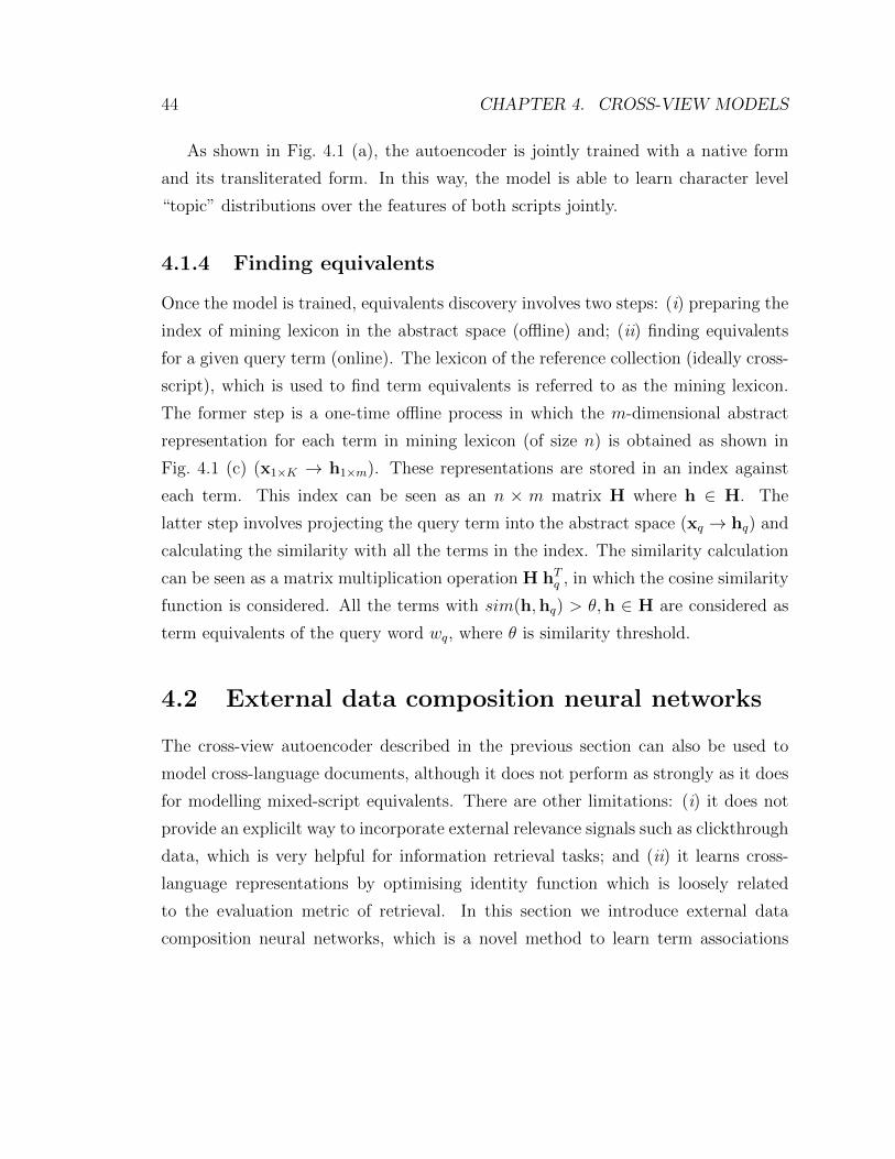
44 CHAPTER 4. CROSS-VIEW MODELS
As shown in Fig. 4.1 (a), the autoencoder is jointly trained with a native form
and its transliterated form. In this way, the model is able to learn character level
“topic” distributions over the features of both scripts jointly.
4.1.4 Finding equivalents
Once the model is trained, equivalents discovery involves two steps: (i) preparing the
index of mining lexicon in the abstract space (offline) and; (ii) finding equivalents
for a given query term (online). The lexicon of the reference collection (ideally cross-
script), which is used to find term equivalents is referred to as the mining lexicon.
The former step is a one-time offline process in which the m-dimensional abstract
representation for each term in mining lexicon (of size n) is obtained as shown in
Fig. 4.1 (c) (x1×K → h1×m). These representations are stored in an index against
each term. This index can be seen as an n × m matrix H where h ∈ H. The
latter step involves projecting the query term into the abstract space (xq → hq) and
calculating the similarity with all the terms in the index. The similarity calculation
can be seen as a matrix multiplication operation H hTq , in which the cosine similarity
function is considered. All the terms with sim(h,hq) > θ,h ∈ H are considered as
term equivalents of the query word wq, where θ is similarity threshold.
4.2 External data composition neural networks
The cross-view autoencoder described in the previous section can also be used to
model cross-language documents, although it does not perform as strongly as it does
for modelling mixed-script equivalents. There are other limitations: (i) it does not
provide an explicilt way to incorporate external relevance signals such as clickthrough
data, which is very helpful for information retrieval tasks; and (ii) it learns cross-
language representations by optimising identity function which is loosely related
to the evaluation metric of retrieval. In this section we introduce external data
composition neural networks, which is a novel method to learn term associations
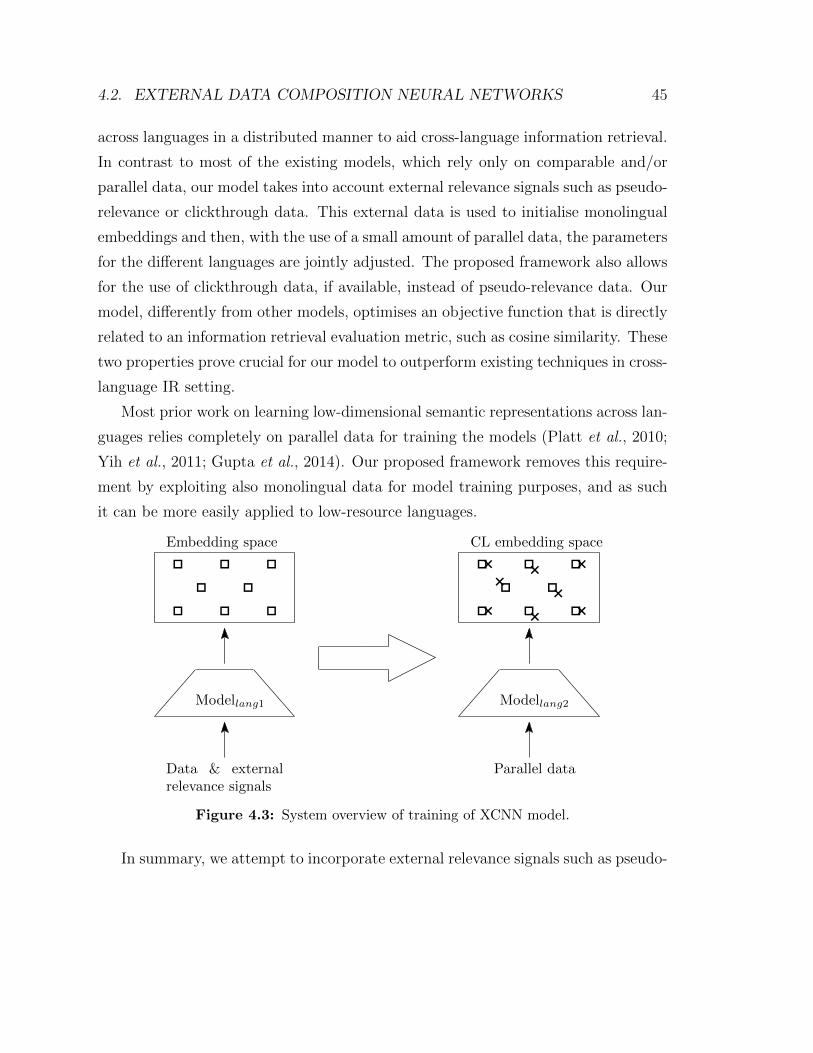
4.2. EXTERNAL DATA COMPOSITION NEURAL NETWORKS 45
across languages in a distributed manner to aid cross-language information retrieval.
In contrast to most of the existing models, which rely only on comparable and/or
parallel data, our model takes into account external relevance signals such as pseudo-
relevance or clickthrough data. This external data is used to initialise monolingual
embeddings and then, with the use of a small amount of parallel data, the parameters
for the different languages are jointly adjusted. The proposed framework also allows
for the use of clickthrough data, if available, instead of pseudo-relevance data. Our
model, differently from other models, optimises an objective function that is directly
related to an information retrieval evaluation metric, such as cosine similarity. These
two properties prove crucial for our model to outperform existing techniques in cross-
language IR setting.
Most prior work on learning low-dimensional semantic representations across lan-
guages relies completely on parallel data for training the models (Platt et al., 2010;
Yih et al., 2011; Gupta et al., 2014). Our proposed framework removes this require-
ment by exploiting also monolingual data for model training purposes, and as such
it can be more easily applied to low-resource languages.
Modellang1
Data & externalrelevance signals
Embedding space
Modellang2
Parallel data
CL embedding space
Figure 4.3: System overview of training of XCNN model.
In summary, we attempt to incorporate external relevance signals such as pseudo-
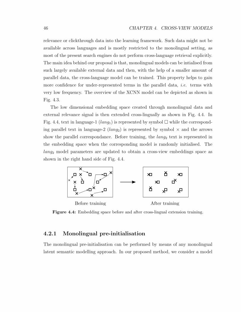
46 CHAPTER 4. CROSS-VIEW MODELS
relevance or clickthrough data into the learning framework. Such data might not be
available across languages and is mostly restricted to the monolingual setting, as
most of the present search engines do not perform cross-language retrieval explicitly.
The main idea behind our proposal is that, monolingual models can be intialised from
such largely available external data and then, with the help of a smaller amount of
parallel data, the cross-language model can be trained. This property helps to gain
more confidence for under-represented terms in the parallel data, i.e. terms with
very low frequency. The overview of the XCNN model can be depicted as shown in
Fig. 4.3.
The low dimensional embedding space created through monolingual data and
external relevance signal is then extended cross-lingually as shown in Fig. 4.4. In
Fig. 4.4, text in language-1 (lang1) is represented by symbol � while the correspond-
ing parallel text in language-2 (lang2) is represented by symbol × and the arrows
show the parallel correspondance. Before training, the lang2 text is represented in
the embedding space when the corresponding model is randomly initialised. The
lang2 model parameters are updated to obtain a cross-view embeddings space as
shown in the right hand side of Fig. 4.4.
Before training After training
Figure 4.4: Embedding space before and after cross-lingual extension training.
4.2.1 Monolingual pre-initialisation
The monolingual pre-initialisation can be performed by means of any monolingual
latent semantic modelling approach. In our proposed method, we consider a model
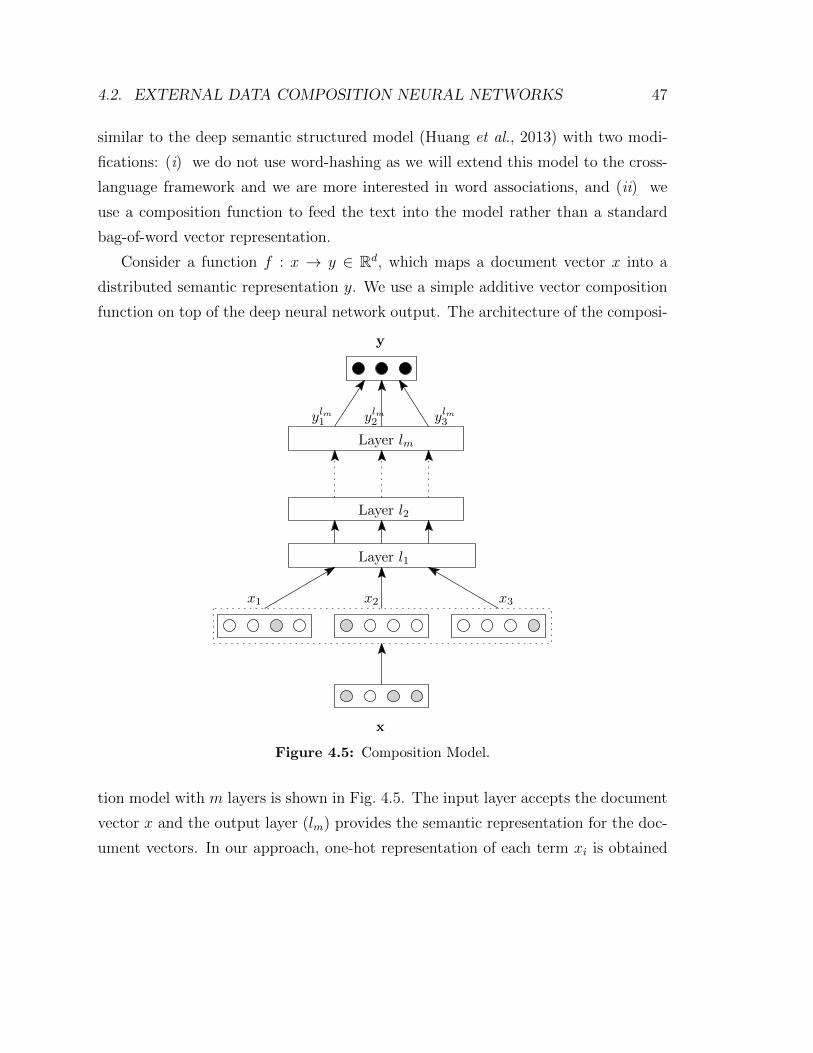
4.2. EXTERNAL DATA COMPOSITION NEURAL NETWORKS 47
similar to the deep semantic structured model (Huang et al., 2013) with two modi-
fications: (i) we do not use word-hashing as we will extend this model to the cross-
language framework and we are more interested in word associations, and (ii) we
use a composition function to feed the text into the model rather than a standard
bag-of-word vector representation.
Consider a function f : x → y ∈ Rd, which maps a document vector x into a
distributed semantic representation y. We use a simple additive vector composition
function on top of the deep neural network output. The architecture of the composi-
x1 x2 x3
y
x
Layer l1
Layer l2
Layer lm
ylm1 ylm2 ylm3
Figure 4.5: Composition Model.
tion model with m layers is shown in Fig. 4.5. The input layer accepts the document
vector x and the output layer (lm) provides the semantic representation for the doc-
ument vectors. In our approach, one-hot representation of each term xi is obtained
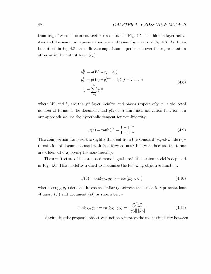
48 CHAPTER 4. CROSS-VIEW MODELS
from bag-of-words document vector x as shown in Fig. 4.5. The hidden layer activ-
ities and the semantic representation y are obtained by means of Eq. 4.8. As it can
be noticed in Eq. 4.8, an additive composition is performed over the representation
of terms in the output layer (lm).
yl1i = g(W1 ∗ xi + b1)
ylji = g(Wj ∗ ylj−1
i + bj), j = 2, ...,m
y =n∑i=1
ylmi
(4.8)
where Wj and bj are the jth layer weights and biases respectively, n is the total
number of terms in the document and g(z) is a non-linear activation function. In
our approach we use the hyperbolic tangent for non-linearity:
g(z) = tanh(z) =1− e−2z
1 + e−2z(4.9)
This composition framework is slightly different from the standard bag-of-words rep-
resentation of documents used with feed-forward neural network because the terms
are added after applying the non-linearity.
The architecture of the proposed monolingual pre-initialisation model is depicted
in Fig. 4.6. This model is trained to maximise the following objective function:
J(θ) = cos(yQ, yD+)− cos(yQ, yD−) (4.10)
where cos(yQ, yD) denotes the cosine similarity between the semantic representations
of query (Q) and document (D) as shown below:
sim(yQ, yD) = cos(yQ, yD) =~yQT ~yD
‖ ~yQ‖‖ ~yD‖(4.11)
Maximising the proposed objective function reinforces the cosine similarity between
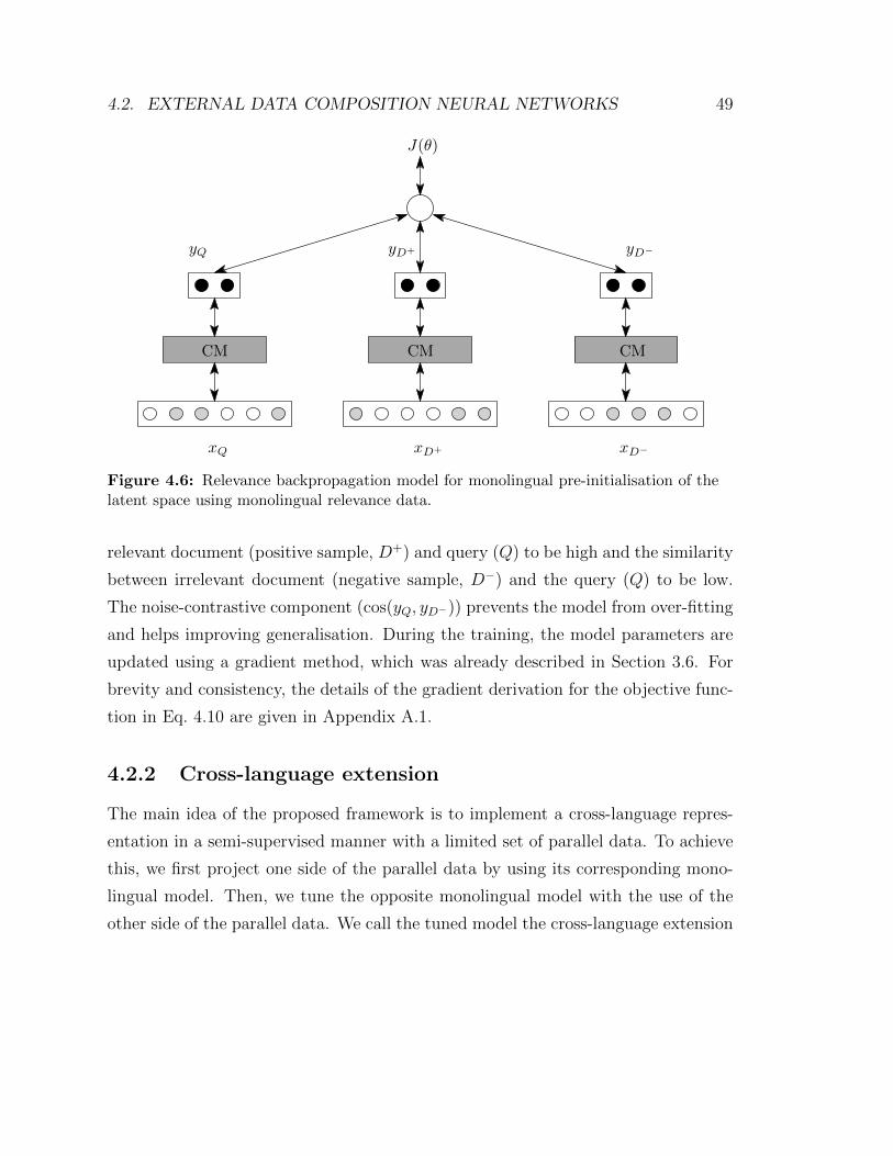
4.2. EXTERNAL DATA COMPOSITION NEURAL NETWORKS 49
xQ xD+ xD−
CM CM CM
J(θ)
yQ yD+ yD−
Figure 4.6: Relevance backpropagation model for monolingual pre-initialisation of thelatent space using monolingual relevance data.
relevant document (positive sample, D+) and query (Q) to be high and the similarity
between irrelevant document (negative sample, D−) and the query (Q) to be low.
The noise-contrastive component (cos(yQ, yD−)) prevents the model from over-fitting
and helps improving generalisation. During the training, the model parameters are
updated using a gradient method, which was already described in Section 3.6. For
brevity and consistency, the details of the gradient derivation for the objective func-
tion in Eq. 4.10 are given in Appendix A.1.
4.2.2 Cross-language extension
The main idea of the proposed framework is to implement a cross-language repres-
entation in a semi-supervised manner with a limited set of parallel data. To achieve
this, we first project one side of the parallel data by using its corresponding mono-
lingual model. Then, we tune the opposite monolingual model with the use of the
other side of the parallel data. We call the tuned model the cross-language extension
50 CHAPTER 4. CROSS-VIEW MODELS
model.
Consider a 3-tuple (yl1 , y+l2, y−l2), where l1 is the language for which we are training
the cross-language extension model, yl1 denotes the distributed representation of
term vector x in l1. On the other hand, y+l2
denotes the distributed representation
of the parallel counterpart of x in l2 and y−l2 is a noise component in l2. The overall
architecture of the model is depicted in Fig. 4.7 and the corresponding objective
function is:
Jcl(θ) = cos(yl1 , y+l2
)− cos(yl1 , y−l2
) (4.12)
xl1 x+l2,x−
l2
CMl1 CMl2
Jcl(θ)
yl1 y+l2 , y−l2
modelbeingtrained
Figure 4.7: Cross-lingual extension model.
The composition models CMl2 are obtained through monolingual pre-initialisation.
In the cross-language extension phase, only the model parameters of CMl1 are up-
dated during the training. The details of the gradient derivation for the objective
function presented in Eq. 4.12 are given in Appendix A.2.

4.2. EXTERNAL DATA COMPOSITION NEURAL NETWORKS 51

Chapter 5Mixed-script information retrieval
For many languages that use non-Roman indigenous scripts (e.g., Arabic, Greek
and Indic languages), one can often find a large amount of transliterated user gener-
ated content on the web in the Roman script. Such content creates a monolingual or
multi-lingual space with more than one script which we refer to as the mixed-script
space. IR in this mixed-script space is challenging because queries written in either
the native or the Roman script need to be matched to the documents written in
both scripts. Moreover, transliterated content features extensive spelling variations.
In this chapter, the concept of mixed-script IR is formally introduced (Section 5.1).
Through analysis of the query logs of Bing search engine, the prevalence and im-
portance of this problem is estimated (Section 5.2). Finally, the experiments and
results on a standard dataset are reported with the proposed model in this thesis
and compared to variety of strong baselines in Sec. 5.3.
53
54 CHAPTER 5. MIXED-SCRIPT INFORMATION RETRIEVAL
5.1 MSIR: Definition & challenges
In this section, the notion of mixed-script IR is formally defined along the lines of
cross-lingual IR (Gupta et al., 2014; Gupta, 2014). A set of research challenges in
the context of MSIR are also presented.
5.1.1 Languages, scripts and transliteration
Let L be a set of (natural) languages {l1, l2, . . . , ln}. Assuming that every language
is generally written using a particular script, which is referred to as the native script
of the language. Let si be the native script for language li. Thus, the set of scripts
S = {s1, s2, . . . , sn} has a one-to-one mapping to L.
Any natural language word w has two attributes: the language it belongs to and
the script it is written in. The notation w ∈ 〈li, sj〉 implies that w is in language li,
written using the script sj. When i = j, word w is considered to be in native script.
Else, in transliterated form, where transliteration can be defined as the process of
loosely or informally representing the sound of a word of one language, li using a
non-native script sj.
Note that a particular language might be traditionally written in more than one
script. For instance, Kurdish is written using the Roman, Cyrillic and Arabic scripts.
However, such cases are rare. On the other hand, it is very common to use a script
for writing several languages. For instance, the Roman script (with slight variations
or additions of diacritics) is used to write English, French, German, Italian, Turkish
and many other languages around the world. Similarly, the Devanagari script is used
for writing Hindi, Sanskrit, Nepali and Marathi languages. Our definition does not
preclude such a possibility, but we would like to emphasise that it is useful to treat
the same script differently when used for writing different languages because the
same sequence of letters might have different pronunciations in different languages.
Consequently, transliterating a word of li (say Hindi) into the scripts sj (say Roman
script as used in English orthography) and sk (say Roman script as used in French
5.1. MSIR: DEFINITION & CHALLENGES 55
orthography) could yield very different results, even though the two scripts use almost
an identical alphabet.
5.1.2 Mixed-script IR
Given a query q and a document pool D, the task of an IR engine is to rank the
documents in D such that the ones relevant to q appear at the top of the ranked
list. Depending on the language in which q and D are presented, one can define two
basic kinds of IR settings. Without loss of generality, let us assume that q ∈ 〈l1, s1〉.In monolingual IR, D = {d1, d2, . . . , dN} consists of only those documents that are
in the same language and script as the query, i.e., for all k, dk ∈ 〈l1, s1〉. This simple
scenario is modified in the context of CLIR, where
D =⋃
i=1...n
Di
where Di = {d1i , d
2i , . . . , d
Ni } are documents in language li, i.e., for all k, dki ∈ 〈li,
si〉. Note that all the documents in a typical CLIR setup are assumed to be written
in the corresponding native scripts.
Based on this fundamental idea of CLIR, a corresponding mixed-script IR setup
can be defined as follows. Let q ∈ 〈l1, sj〉 be a query, where j may or may not be
equal to 1. The document pool,
D =⋃
k=1...n
Dk1
where Dk1 = {dk,11 , dk,21 , . . . , dk,N1 } are documents in language l1 written in script
sk, i.e., for all m, dk,m1 ∈ 〈l1, sk〉. In other words, in the MSIR setup, the query and
the documents are all in the same language, say l1, but they are written in more
than one different scripts. The task of the IR engine is to search across the scripts.
In the literature, sometimes CLIR is distinguished from multilingual IR in the
sense that the former refers to a case where n = 2, whereas the latter is a gener-
56 CHAPTER 5. MIXED-SCRIPT INFORMATION RETRIEVAL
alization to any n > 2. Likewise, for monolingual IR, n can be assumed to be 1.
One could make a similar distinction between mono-script, cross-Script and mixed-
script IR scenarios, where the query and the documents are in one language, but in
1, 2 or more than 2 scripts respectively. Nevertheless, we will refer to both latter
cases as MSIR. All the experiments involve a single language, namely Hindi, and two
scripts – Devanagari and the Roman script (English orthography) – but the proposed
approach can be easily extended to a larger set of scripts.
One can also further generalise the setup to mixed-script multilingual IR, where
q as well as D can be in one of several languages and written in one of several scripts.
This is also a useful and practical setup, though we will not discuss it any further in
this work.
It should also be noted that, like in CLIR, in the MSIR setting it is possible that
for q ∈ {li, sj}, the information might be available only in a dj′,ki where i 6= j′. In
such cases, often the users issuing the query might be able to read and write both sj
and sj′ and hence dj′,ki would have solved users information need. However, without
MSIR this would not be possible to achieve.
5.1.3 Mixed and transliterated queries & documents
The definition of the MSIR setup assumes that the entire query and each document
are in a single language and single script. However, in practice, one can find queries
or documents that contain text fragments written in more than one language or script
or both. Furthermore, depending on whether the parts of a query or document are
written in a language using the native or a non-native script, one can have native or
transliterated queries and documents.
A practical way to address the issue of mixed-script within documents could be
to split them into several sub-documents such that each of the sub-documents are in
a single language and single script as discussed in Choudhury et al. (2012), given the
mixing is not at the sub-sentence level which falls under the different case of code-
mixing. Mixed queries, however, cannot be handled through simple splitting because
5.1. MSIR: DEFINITION & CHALLENGES 57
matching parts of a query to the documents does not make sense in the context of
IR. Therefore, the MSIR setup is extended to include mixed queries. Let a query q
be defined as a string of words w1w2 . . . wm, where w1 ∈ 〈li1 , sj1〉, w2 ∈ 〈li2 , sj2〉 and
so on can all belong to different languages, scripts or both.
5.1.4 Challenges in MSIR
The two primary challenges in MSIR are: (i) how to tackle the extensive spelling
variations in the transliterated queries and documents during the term matching
phase, and (ii) how to identify, process and represent a mixed query (and also, the
mixed and transliterated documents). In CLIR, there are broadly two approaches:
(i) to model the cross-lingual space, either documents and queries are translated
to bring all words into the same monolingual space, after which monolingual IR
techniques and matching algorithms can be directly applied; or (ii) the cross-lingual
space is modelled jointly as an abstract topic or semantic space, and documents and
queries in all languages are mapped to this common space. Likewise, in MSIR one
can “transliterate” the text to bring everything into a common space and then apply
standard matching techniques in the single-script space, or one can jointly model an
abstract orthographic space for representing the words written in different scripts.
In this thesis, we explore the latter, which we believe is a more robust and generic
solution to the mixed-script space modelling problem, as it can simultaneously handle
spelling variations in a single script and across multiple scripts.
Mixed query processing is another interesting research challenge, which includes
language identification of the query words, which can be either in native or transliter-
ated scripts, and labeling those with semantic or other tags (e.g., entities, attributes).
This is challenging mainly because, depending on the context of the query, the same
string, say “man”, could represent the English word man, a transliterated Hindi word
man meaning “mind”, or another transliterated Hindi word maan meaning “repu-
tation”. In addition, the same word with similar meanings are also used in many
other Indian languages and can have different connotations in other languages (e.g.,
58 CHAPTER 5. MIXED-SCRIPT INFORMATION RETRIEVAL
in Bengali this could also mean “to get offended”). Hence, language identification
seems to be an extremely challenging problem in the MSIR setting, especially when
multiple languages are involved. In this work, we limit our experiments to only two
languages, namely English and Hindi, and describe some initial results with language
identification for transliterated and mixed queries.
Apart from these basic challenges, result presentation in MSIR is also an inter-
esting problem because this requires the information on whether the user can read
all the scripts, or prefer some scripts over others. There are no user studies related
to MSIR, which is ripe with several such open problems.
5.2 Transliterated queries in web search
Although the current web search engines do not support MSIR, they still have to
handle a large traffic of mixed and transliterated queries from linguistic regions that
use non-Roman indigenous scripts. To better understand the distribution of trans-
literated queries across various topics and domains, an analysis of mixed and trans-
literated queries extracted from a large query log of Bing is presented. This could
provide deeper understanding of the MSIR space and its users. This analysis relies
on automatic identification and classification techniques for mixed queries developed
specifically for this task.
5.2.1 Methodology
The analysis is conducted on 13.78 billion queries sampled from the logs of Bing on
real user searches conducted in India. India provides an interesting socio-linguistic
context for studying mixed queries because of the abundance of Roman translitera-
tions and the multiplicity of languages and scripts. This dataset consists of 30 million
unique queries with an average length of 4.32 words per query. Almost all the queries
(99.998%) are in Roman script (but not necessarily in English language). For ease
of computation, we randomly sampled 1% (i.e., 300,000) of the unique queries and
5.2. TRANSLITERATED QUERIES IN WEB SEARCH 59
conducted the study on this smaller sample. The analysis is carried out in successive
steps, which are explained below.
Step-1: Language identification In order to identify the mixed-script queries,
a language identification classifier was trained. The classifier is based on a maximum
entropy model, which uses character n-gram features (n = 1 to 5). Training was
carried out with 5000 labelled words for each language. Hindi words were top trans-
literated words from Bollywood songs lyrics obtained through Gupta et al. (2012a)
and English words from the Leipzig Corpus1. On 2500 unseen words, the accuracy of
the classifier was measured to be 97%. The language identification was carried out
based on a similar word-level identification task in King and Abney (2013). With this
classifier, a query q is considered to be mixed-script or transliterated if it contains
more than 40% words classified as Hindi.
Step-2: Query categories After analysing the transliterated queries identified in
Step-1, six broad categories or topics were identified: Named Entities, Entertainment,
Information Source, Culture, Recipe and Research. Each of these were further refined
into a set of sub-categories; e.g., Named Entities can be of three types people, location
and organisation. Besides, we also observed a few interesting subcategories, which
we put together under a catch-all seventh category – Others. Table 5.1 lists all these
categories and sub-categories along with example queries.
Step-3: Category assignment In order to automatically classify the queries
into these categories, we resort to a simple minimally supervised approach. Through
manual inspection of the transliterated queries, five representative and reasonably
frequent examples for each sub-category were selected. All the queries from the data-
set that have at least one word in common with at least one of the five representative
queries were extracted. Then, the top 100 most frequent words in this set of quer-
ies were populated. The standard English stopwords were removed from these 100
1http://corpora.uni-leipzig.de/
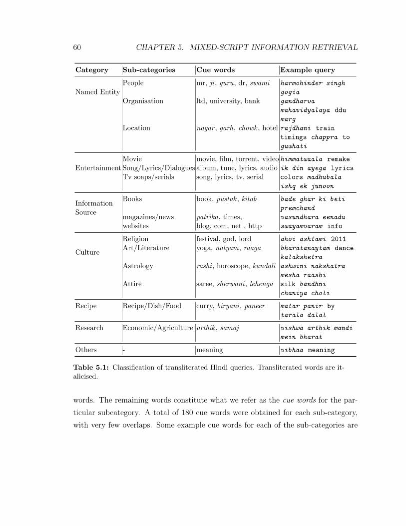
60 CHAPTER 5. MIXED-SCRIPT INFORMATION RETRIEVAL
Category Sub-categories Cue words Example query
Named EntityPeople mr, ji , guru, dr, swami harmohinder singh
gogia
Organisation ltd, university, bank gandharva
mahavidyalaya ddu
marg
Location nagar , garh, chowk , hotel rajdhani train
timings chappra to
guwhati
EntertainmentMovie movie, film, torrent, video himmatwaala remake
Song/Lyrics/Dialogues album, tune, lyrics, audio ik din ayega lyrics
Tv soaps/serials song, lyrics, tv, serial colors madhubala
ishq ek junoon
InformationSource
Books book, pustak , kitab bade ghar ki beti
premchand
magazines/news patrika, times, vasundhara eenadu
websites blog, com, net , http swayamvaram info
Culture
Religion festival, god, lord ahoi ashtami 2011
Art/Literature yoga, natyam, raaga bharatanaytam dance
kalakshetra
Astrology rashi , horoscope, kundali ashwini nakshatra
mesha raashi
Attire saree, sherwani , lehenga silk bandhni
chaniya choli
Recipe Recipe/Dish/Food curry, biryani , paneer matar panir by
tarala dalal
Research Economic/Agriculture arthik , samaj vishwa arthik mandi
mein bharat
Others - meaning vibhaa meaning
Table 5.1: Classification of transliterated Hindi queries. Transliterated words are it-alicised.
words. The remaining words constitute what we refer as the cue words for the par-
ticular subcategory. A total of 180 cue words were obtained for each sub-category,
with very few overlaps. Some example cue words for each of the sub-categories are
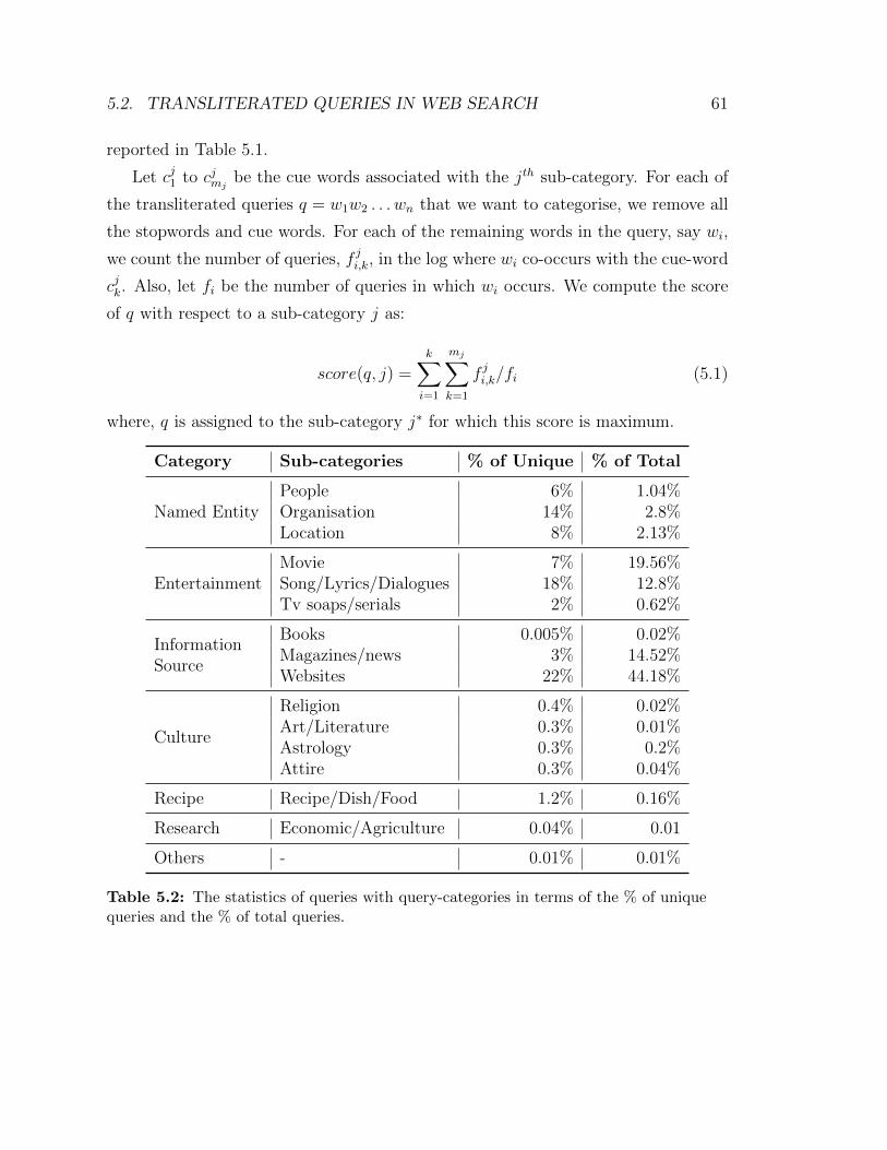
5.2. TRANSLITERATED QUERIES IN WEB SEARCH 61
reported in Table 5.1.
Let cj1 to cjmjbe the cue words associated with the jth sub-category. For each of
the transliterated queries q = w1w2 . . . wn that we want to categorise, we remove all
the stopwords and cue words. For each of the remaining words in the query, say wi,
we count the number of queries, f ji,k, in the log where wi co-occurs with the cue-word
cjk. Also, let fi be the number of queries in which wi occurs. We compute the score
of q with respect to a sub-category j as:
score(q, j) =k∑i=1
mj∑k=1
f ji,k/fi (5.1)
where, q is assigned to the sub-category j∗ for which this score is maximum.
Category Sub-categories % of Unique % of Total
Named EntityPeople 6% 1.04%Organisation 14% 2.8%Location 8% 2.13%
EntertainmentMovie 7% 19.56%Song/Lyrics/Dialogues 18% 12.8%Tv soaps/serials 2% 0.62%
InformationSource
Books 0.005% 0.02%Magazines/news 3% 14.52%Websites 22% 44.18%
Culture
Religion 0.4% 0.02%Art/Literature 0.3% 0.01%Astrology 0.3% 0.2%Attire 0.3% 0.04%
Recipe Recipe/Dish/Food 1.2% 0.16%
Research Economic/Agriculture 0.04% 0.01
Others - 0.01% 0.01%
Table 5.2: The statistics of queries with query-categories in terms of the % of uniquequeries and the % of total queries.
62 CHAPTER 5. MIXED-SCRIPT INFORMATION RETRIEVAL
5.2.2 Observations
In our dataset, as much as 6% of the unique queries were identified as transliterated,
which means that at least 40% of the words in these queries are Roman translitera-
tions of Hindi words. The average query length for the transliterated queries is 2.86,
which is less than 4.32 – the average query length of all queries. The frequency of
the transliterated queries are in general less than that of the non-transliterated ones.
Hence, they only constitute about 0.011% of all the queries in our dataset. However,
their frequency distribution follows the same power-law pattern as the regular quer-
ies, albeit spanning mainly the medium and low frequency spectra. This also implies
that a large number of transliterated and mixed queries belong to the long tail of
the overall query distribution and may not have enough clickthrough data to help a
search engine process them accurately. Because of this, they must be processed dif-
ferently, recognizing the fact that they are rare, but together they do form a sizeable
mass of the search traffic.
Table 5.2 presents the distribution statistics of the transliterated queries in each
of the identified sub-categories. The numbers do not add to 100% because a small
fraction of queries, 18% of unique but only 2% of all, could not be mapped to any
of the categories. It is not surprising that a large fraction of the queries are NEs.
Along with Websites, NEs form 50% of the unique queries, though when query fre-
quencies are taken into account NEs only constitute 6% of all queries. Consequently,
processing of transliterated NEs has received some attention from the IR research-
ers (Kumaran et al., 2010). Entertainment is the second largest category (27%), of
which movies and songs are the most searched categories. These queries are typic-
ally longer and more complex than NE queries, and constitute more than 32% of
the transliterated query traffic. Yet, this category has hardly received any special
attention from the researchers (Dua et al., 2011; Gupta et al., 2012a). We believe
that Entertainment is a rich and practically important domain for MSIR, and hence
we conduct our MSIR experiments on Hindi song lyrics dataset (Saha Roy et al.,
2013).
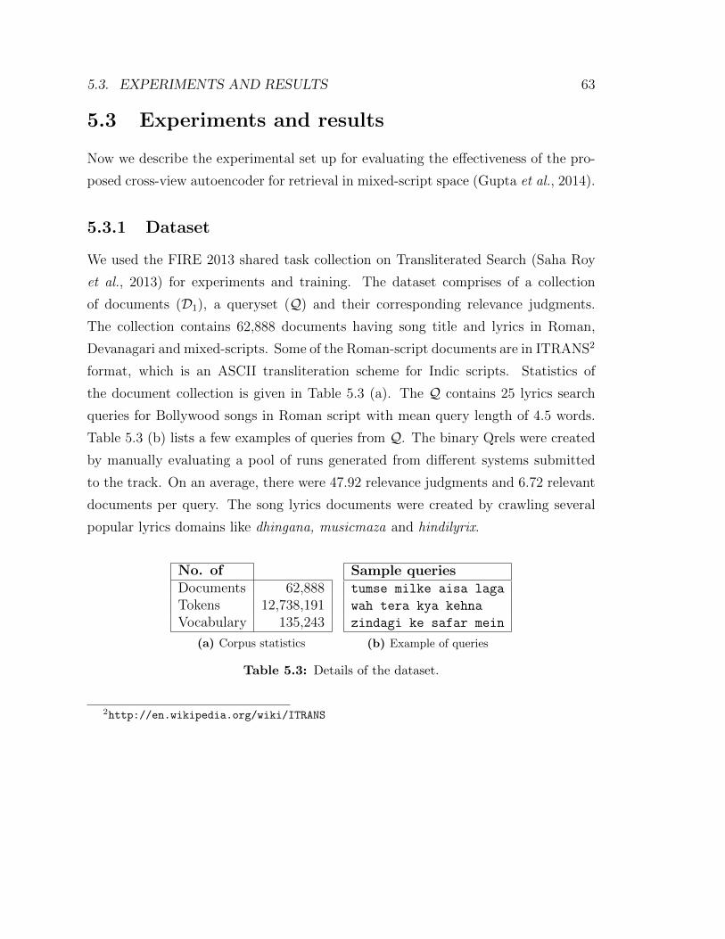
5.3. EXPERIMENTS AND RESULTS 63
5.3 Experiments and results
Now we describe the experimental set up for evaluating the effectiveness of the pro-
posed cross-view autoencoder for retrieval in mixed-script space (Gupta et al., 2014).
5.3.1 Dataset
We used the FIRE 2013 shared task collection on Transliterated Search (Saha Roy
et al., 2013) for experiments and training. The dataset comprises of a collection
of documents (D1), a queryset (Q) and their corresponding relevance judgments.
The collection contains 62,888 documents having song title and lyrics in Roman,
Devanagari and mixed-scripts. Some of the Roman-script documents are in ITRANS2
format, which is an ASCII transliteration scheme for Indic scripts. Statistics of
the document collection is given in Table 5.3 (a). The Q contains 25 lyrics search
queries for Bollywood songs in Roman script with mean query length of 4.5 words.
Table 5.3 (b) lists a few examples of queries from Q. The binary Qrels were created
by manually evaluating a pool of runs generated from different systems submitted
to the track. On an average, there were 47.92 relevance judgments and 6.72 relevant
documents per query. The song lyrics documents were created by crawling several
popular lyrics domains like dhingana, musicmaza and hindilyrix.
No. ofDocuments 62,888Tokens 12,738,191Vocabulary 135,243
(a) Corpus statistics
Sample queriestumse milke aisa laga
wah tera kya kehna
zindagi ke safar mein
(b) Example of queries
Table 5.3: Details of the dataset.
2http://en.wikipedia.org/wiki/ITRANS
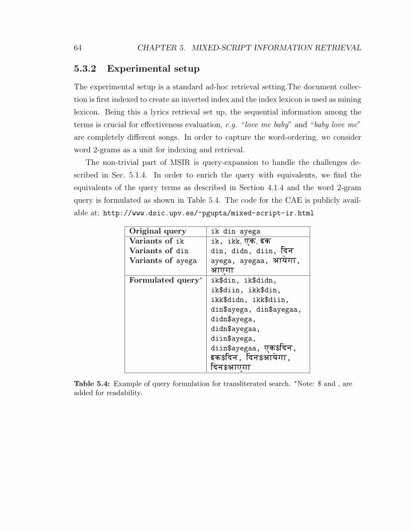
64 CHAPTER 5. MIXED-SCRIPT INFORMATION RETRIEVAL
5.3.2 Experimental setup
The experimental setup is a standard ad-hoc retrieval setting.The document collec-
tion is first indexed to create an inverted index and the index lexicon is used as mining
lexicon. Being this a lyrics retrieval set up, the sequential information among the
terms is crucial for effectiveness evaluation, e.g. “love me baby” and “baby love me”
are completely different songs. In order to capture the word-ordering, we consider
word 2-grams as a unit for indexing and retrieval.
The non-trivial part of MSIR is query-expansion to handle the challenges de-
scribed in Sec. 5.1.4. In order to enrich the query with equivalents, we find the
equivalents of the query terms as described in Section 4.1.4 and the word 2-gram
query is formulated as shown in Table 5.4. The code for the CAE is publicly avail-
able at: http://www.dsic.upv.es/~pgupta/mixed-script-ir.html
Original query ik din ayega
Variants of ik ik, ikk, ek, ikVariants of din din, didn, diin, EdnVariants of ayega ayega, ayegaa, aAy�gA,
aAegAFormulated query∗ ik$din, ik$didn,
ik$diin, ikk$din,ikk$didn, ikk$diin,din$ayega, din$ayegaa,didn$ayega,didn$ayegaa,diin$ayega,diin$ayegaa, ek$Edn,ik$Edn, Edn$aAy�gA,Edn$aAegA
Table 5.4: Example of query formulation for transliterated search. ∗Note: $ and , areadded for readability.
5.3. EXPERIMENTS AND RESULTS 65
5.3.3 Baseline systems
We consider a variety of baseline systems and compared them with the proposed
method. The query formulation is similar for all the systems including the retrieval
settings like inverted index, retrieval model and mining lexicon, except the method
for finding the equivalents.
1. Naıve: The original query terms are used for the query formulation without
any query-enrichment step.
2. Naıve + Trans: The original query terms and their automatic back-transliteration
obtained from a commercial transliteration engine3 are used for query formu-
lation.
3. CL-LSI: In this system, linear dimensionality reduction technique known as
cross-language latent semantic indexing (Dumais et al., 1997) is used to learn
the low-dimensional embedding of the terms across the scripts. Consider mat-
rix An×K where aij is the count data of jth feature fj ∈ F in ith training
word-pair. Such matrix A is factored using CL-LSI to learn projection matrix
(VK×m) such that hq = xqV . The equivalents of the query term t are obtained
from 50-dimensional abstract space as described in Section 4.1.4. Thus found
equivalents, along with original query terms, are used for query formulation.
4. Editex: An approximate string matching algorithm for IR proposed in Zobel
and Dart (1996) is used to get equivalents of the query term. Editex uses
advanced Phonix and Soundex information to normalise the pronunciation dif-
ferences. The distance between such normalised strings is calculated as edit
distance. Editex can handle strings only in Roman alphabet. Therefore, only
Roman script equivalents of the query terms are found using Editex.
5. CCA: In this case, the problem of finding equivalents is formulated as search
problem across the different views by learning hashing functions (Kumar and
3Yahoo! Transliteration: http://transliteration.yahoo.com/
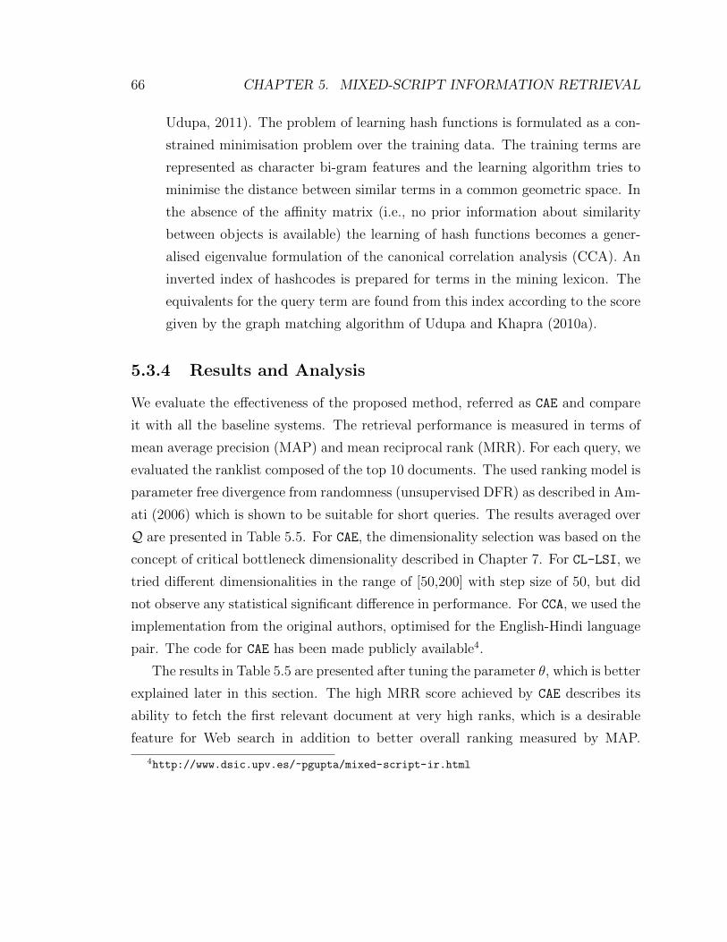
66 CHAPTER 5. MIXED-SCRIPT INFORMATION RETRIEVAL
Udupa, 2011). The problem of learning hash functions is formulated as a con-
strained minimisation problem over the training data. The training terms are
represented as character bi-gram features and the learning algorithm tries to
minimise the distance between similar terms in a common geometric space. In
the absence of the affinity matrix (i.e., no prior information about similarity
between objects is available) the learning of hash functions becomes a gener-
alised eigenvalue formulation of the canonical correlation analysis (CCA). An
inverted index of hashcodes is prepared for terms in the mining lexicon. The
equivalents for the query term are found from this index according to the score
given by the graph matching algorithm of Udupa and Khapra (2010a).
5.3.4 Results and Analysis
We evaluate the effectiveness of the proposed method, referred as CAE and compare
it with all the baseline systems. The retrieval performance is measured in terms of
mean average precision (MAP) and mean reciprocal rank (MRR). For each query, we
evaluated the ranklist composed of the top 10 documents. The used ranking model is
parameter free divergence from randomness (unsupervised DFR) as described in Am-
ati (2006) which is shown to be suitable for short queries. The results averaged over
Q are presented in Table 5.5. For CAE, the dimensionality selection was based on the
concept of critical bottleneck dimensionality described in Chapter 7. For CL-LSI, we
tried different dimensionalities in the range of [50,200] with step size of 50, but did
not observe any statistical significant difference in performance. For CCA, we used the
implementation from the original authors, optimised for the English-Hindi language
pair. The code for CAE has been made publicly available4.
The results in Table 5.5 are presented after tuning the parameter θ, which is better
explained later in this section. The high MRR score achieved by CAE describes its
ability to fetch the first relevant document at very high ranks, which is a desirable
feature for Web search in addition to better overall ranking measured by MAP.
4http://www.dsic.upv.es/~pgupta/mixed-script-ir.html
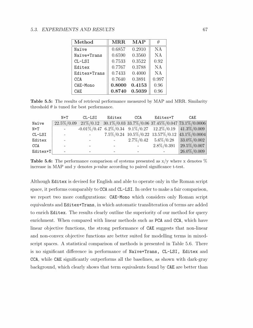
5.3. EXPERIMENTS AND RESULTS 67
Method MRR MAP θ
Naıve 0.6857 0.2910 NANaıve+Trans 0.6590 0.3560 NACL-LSI 0.7533 0.3522 0.92Editex 0.7767 0.3788 NAEditex+Trans 0.7433 0.4000 NACCA 0.7640 0.3891 0.997CAE-Mono 0.8000 0.4153 0.96CAE 0.8740 0.5039 0.96
Table 5.5: The results of retrieval performance measured by MAP and MRR. Similaritythreshold θ is tuned for best performance.
N+T CL-LSI Editex CCA Editex+T CAE
Naıve 22.5%/0.09 21%/0.12 30.1%/0.03 33.7%/0.06 37.45%/0.047 73.1%/0.0006N+T - -0.01%/0.47 6.2%/0.34 9.1%/0.27 12.2%/0.19 41.3%/0.009CL-LSI - - 7.5%/0.24 10.5%/0.22 13.57%/0.12 43.1%/0.0004Editex - - - 2.7%/0.42 5.6%/0.28 33.0%/0.002CCA - - - - 2.8%/0.391 29.5%/0.007Editex+T - - - - - 26.0%/0.009
Table 5.6: The performance comparison of systems presented as x/y where x denotes %increase in MAP and y denotes p-value according to paired significance t-test.
Although Editex is devised for English and able to operate only in the Roman script
space, it performs comparably to CCA and CL-LSI. In order to make a fair comparison,
we report two more configurations: CAE-Mono which considers only Roman script
equivalents and Editex+Trans, in which automatic transliteration of terms are added
to enrich Editex. The results clearly outline the superiority of our method for query
enrichment. When compared with linear methods such as PCA and CCA, which have
linear objective functions, the strong performance of CAE suggests that non-linear
and non-convex objective functions are better suited for modelling terms in mixed-
script spaces. A statistical comparison of methods is presented in Table 5.6. There
is no significant difference in performance of Naıve+Trans, CL-LSI, Editex and
CCA, while CAE significantly outperforms all the baselines, as shown with dark-gray
background, which clearly shows that term equivalents found by CAE are better than
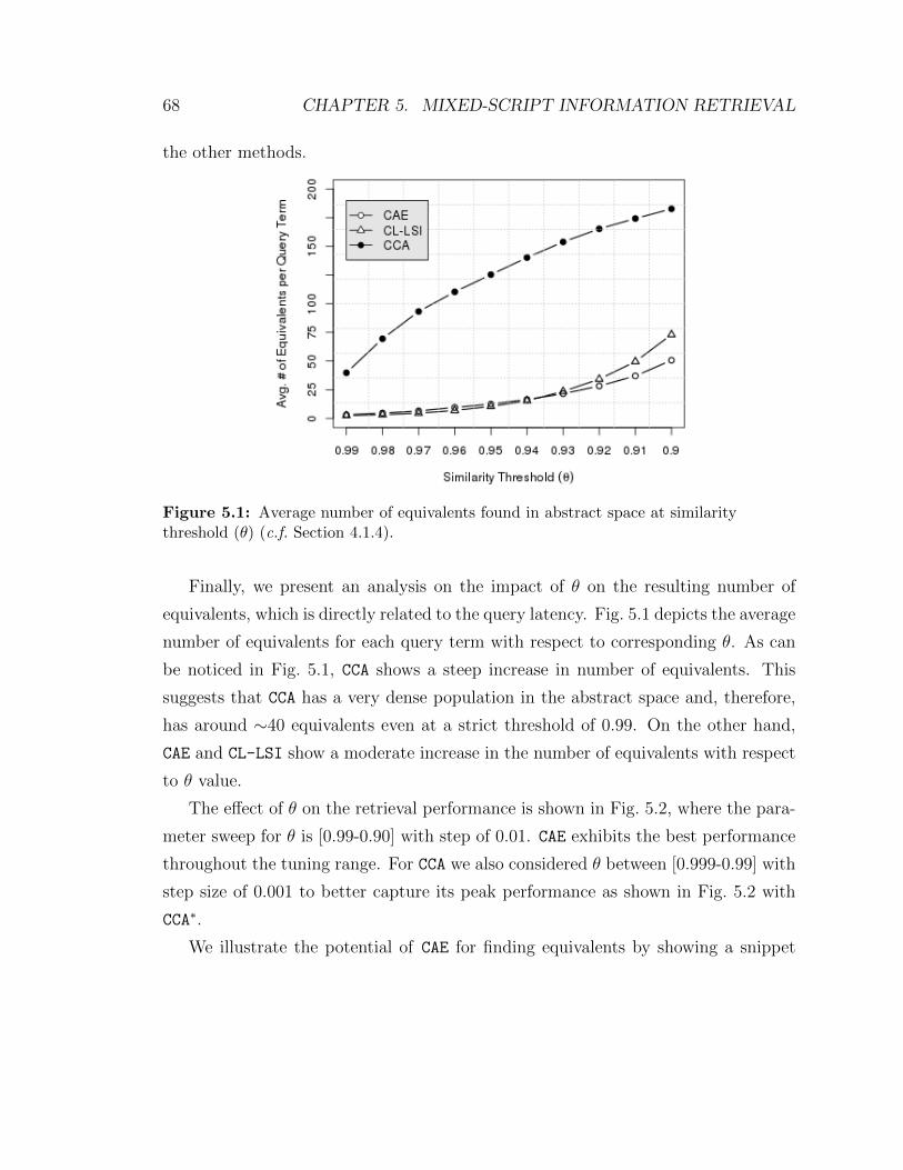
68 CHAPTER 5. MIXED-SCRIPT INFORMATION RETRIEVAL
the other methods.
Figure 5.1: Average number of equivalents found in abstract space at similaritythreshold (θ) (c.f. Section 4.1.4).
Finally, we present an analysis on the impact of θ on the resulting number of
equivalents, which is directly related to the query latency. Fig. 5.1 depicts the average
number of equivalents for each query term with respect to corresponding θ. As can
be noticed in Fig. 5.1, CCA shows a steep increase in number of equivalents. This
suggests that CCA has a very dense population in the abstract space and, therefore,
has around ∼40 equivalents even at a strict threshold of 0.99. On the other hand,
CAE and CL-LSI show a moderate increase in the number of equivalents with respect
to θ value.
The effect of θ on the retrieval performance is shown in Fig. 5.2, where the para-
meter sweep for θ is [0.99-0.90] with step of 0.01. CAE exhibits the best performance
throughout the tuning range. For CCA we also considered θ between [0.999-0.99] with
step size of 0.001 to better capture its peak performance as shown in Fig. 5.2 with
CCA∗.
We illustrate the potential of CAE for finding equivalents by showing a snippet
5.3. EXPERIMENTS AND RESULTS 69
Figure 5.2: Impact of similarity threshold (θ) on retrieval performance. CCA∗ followsthe ceiling X-axis range [0.999-0.99].
of 20D abstract space as a 2D-view in Fig. 5.3. It can be noticed that mixed-script
equivalents of the terms are very close to each other in small clusters and such clusters
are well separated from each other. The 2D representation is achieved using the t-
SNE algorithm5. We show equivalents of a few terms found using CAE with θ=0.96
in Table 5.7. The category “not sure” depicts the cases where the terms are quite
close to the desired term but not correct, which may be due to a typo e.g. ehaas vs.
ehsaas where the former is not a valid Hindi word.
5.3.5 Scalability
Among the two steps involved in finding equivalents listed in Sec. 4.1.4, the indexing
step, being one-time and offline, is not a major concern. On the contrary, the real
time similarity estimation during the online step while searching for equivalents is
5http://homepage.tudelft.nl/19j49/t-SNE.html
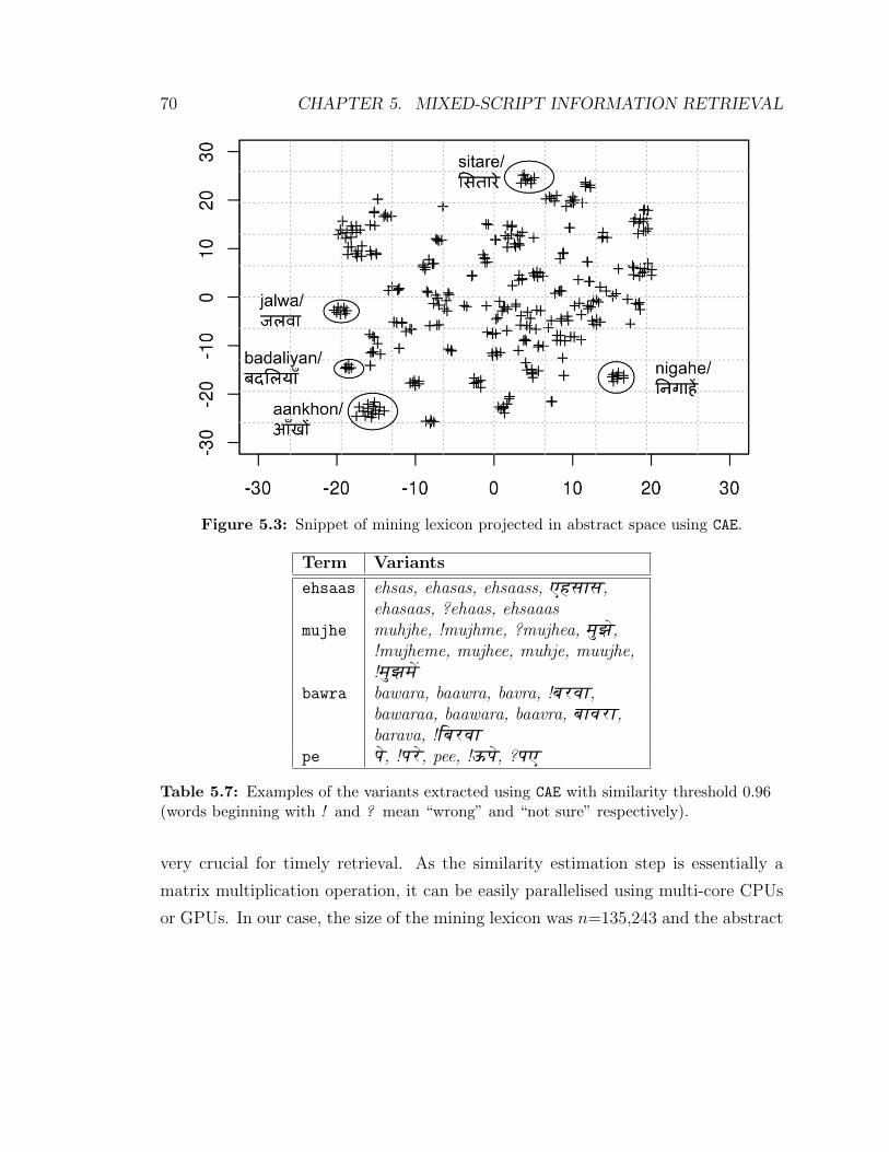
70 CHAPTER 5. MIXED-SCRIPT INFORMATION RETRIEVAL
Figure 5.3: Snippet of mining lexicon projected in abstract space using CAE.
Term Variants
ehsaas ehsas, ehasas, ehsaass, ehsAs,ehasaas, ?ehaas, ehsaaas
mujhe muhjhe, !mujhme, ?mujhea, m� J�,!mujheme, mujhee, muhje, muujhe,!m� Jm�\
bawra bawara, baawra, bavra, !brvA,bawaraa, baawara, baavra, bAvrA,barava, !EbrvA
pe p�, !pr�, pee, !Up�, ?pe
Table 5.7: Examples of the variants extracted using CAE with similarity threshold 0.96(words beginning with ! and ? mean “wrong” and “not sure” respectively).
very crucial for timely retrieval. As the similarity estimation step is essentially a
matrix multiplication operation, it can be easily parallelised using multi-core CPUs
or GPUs. In our case, the size of the mining lexicon was n=135,243 and the abstract
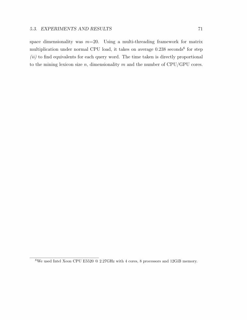
5.3. EXPERIMENTS AND RESULTS 71
space dimensionality was m=20. Using a multi-threading framework for matrix
multiplication under normal CPU load, it takes on average 0.238 seconds6 for step
(ii) to find equivalents for each query word. The time taken is directly proportional
to the mining lexicon size n, dimensionality m and the number of CPU/GPU cores.
6We used Intel Xeon CPU E5520 @ 2.27GHz with 4 cores, 8 processors and 12GiB memory.

Chapter 6Cross-language information retrieval
Cross-language information retrieval refers to the scenario of accepting informa-
tion need in one language and retrieving relevant information in a different language.
An information need can be in form of a document, a natural language question or
simply a search query.
This chapter aims at applying the CAE (c.f. Section 4.1) and XCNN (c.f. Sec-
tion 4.2) models to various task of cross-language information retrieval. First, we give
an overview of a set of existing cross-language text similarity assessment strategies
and then explain a few models that are used in this dissertation in Section 6.1.
The problem statement, experimental setup and results for different CLIR tasks
are presented in the successive sections: cross-language plagiarism detection (Sec-
tion 6.2), cross-language ad-hoc retrieval (Section 6.3), parallel sentence retrieval (Sec-
tion 6.4) and source sentence retrieval for machine translation (Section 6.5).
73
74 CHAPTER 6. CROSS-LANGUAGE INFORMATION RETRIEVAL
6.1 Cross-language text similarity
In general, cross-language text similarity methods can be categorised into following
six categories.
(i) Lexical-based systems rely on vocabulary similarity (e.g. English–French)
and linguistic influence (e.g. English computer → Spanish computadora) between
languages. Similarities across words in different languages can be reflected when
composing short terms; e.g. character n-grams or prefixes. Probably two of the first
similarity models of this kind are cognateness – based on prefixes and other tokens
– (Simard et al., 1992) and dot-plot – based on character 4-grams (Church, 1993).
While originally proposed to align bitexts, these models are useful to measure simil-
arity across languages (Potthast et al., 2011), but still with some limitations (Barron-
Cedeno et al., 2010).
(ii) Thesauri-based systems map words or concepts, such as named entities,
into a common representation space by means of a multilingual thesaurus, such as
Eurovoc (Steinberger et al., 2002; Gupta et al., 2012b) or EuroWordnet (Vossen,
1998). However, multilingual thesauri are not always a viable solution. For in-
stance, Ceska et al. (2008) found that the incompleteness of the thesaurus (in that
case EuroWordnet) may limit the detection capabilities. Multilingual semantic net-
work – BabelNet (Navigli and Ponzetto, 2012) based cross-language knowledge graph
analysis (CL-KGA) provides a framework to estimate these similarities in the graph
space (Franco-Salvador et al., 2013).
(iii) Comparable corpus-based systems are trained over comparable corpora.
One example is cross-language explicit semantic analysis (Potthast et al., 2008).
Given documents (dq and d′) are represented by a vector of similarities to the doc-
uments of a so-called CL index collection CI , i.e., ~dq = {sim(dq, c1), . . . sim(dq, cI)},~d′ = {sim(d′, c′1), . . . sim(d′, c′I)}, where, (ci ∈ L and c′i ∈ L′ are comparable docu-
6.1. CROSS-LANGUAGE TEXT SIMILARITY 75
ments). Here, sim is a monolingual similarity model, such as the cosine measure. ~dq
and ~d′ are then compared to compute sim(dq, d′).
(iv) Parallel corpus-based systems are trained on parallel corpora, either to
find cross-language co-occurrences (Littman et al., 1998) or to obtain translation
modules. The principles and resources of machine translation are used, but no actual
translations are computed. Cross-language alignment-based similarity analysis is one
of such models and it is discussed in more detail in Section 6.1.3.
(v) Machine translation-based systems simplify the problem by turning it into
a monolingual problem. The main approach is as follows: (i) a language detector is
applied to determine the most likely language of the documents at hand; (ii) if not
written in the comparison language, one of the documents is translated; and (iii) a
monolingual comparison is carried out between the two documents.
(vi) Translingual continuous space systems learn continuous space represent-
ation for text across languages and measure similarity in this space. Models such
as cross-language latent semantic indexing (Dumais et al., 1997) and oriented prin-
ciple component analysis (Platt et al., 2010) learn linear projections for text through
matrix factorization methods. While S2Net (Yih et al., 2011) uses a Siamese neural
network to learn the projections. The models proposed in this thesis, CAE and
XCNN, also fall in this category.
Now, we present a few models that can be used for cross-language text similarity.
6.1.1 Cross-language character n-grams (CL-CNG)
Cross-language character n-grams was originally proposed by Mcnamee and May-
field (2004) for cross-language information retrieval. It is a very simple model that
decomposes the text from two language sources into smaller units such as charac-
ter n-grams. Standard normalisation techniques are applied such as lower-casing
76 CHAPTER 6. CROSS-LANGUAGE INFORMATION RETRIEVAL
and diacritics removal. Following Potthast et al. (2011), we used n = 3 for our
experiments. The similarity between text representations is computed using cosine
similarity.
6.1.2 Cross-language explicit semantic analysis (CL-ESA)
Cross-language explicit semantic analysis (Potthast et al., 2008) extends the explicit
semantic analysis model (Gabrilovich and Markovitch, 2007) to work in a cross-
language scenario. This model represents each text by means of its similarities with
a document collection D. Even though the indexing with D is performed at mono-
lingual level, using a multilingual document collections with comparable documents
across languages, e.g. Wikipedia1, allows for the resulting vectors from different
languages to be compared. Formally, having a matrix DL where rows represent
documents of a collection in a language L, a document dL is indexed as follows:
dDL= DL · dTL, (6.1)
where dDLdenotes the resulting indexed vector of document dL in DL. Docu-
ments represented in dL and DL use a vector representation such as VSM with term
frequency-inverse document frequency (TF-IDF) weighting (Salton et al., 1983). The
similarity between two documents dL and d′L′ is estimated as ϕ(dDL, d′DL′
), where ϕ
is a vector similarity function, and DL and DL′ are comparable document collections
between L and L′.
6.1.3 Cross-language alignment-based similarity analysis (CL-
ASA)
Cross-language alignment-based similarity analysis (Barron-Cedeno et al., 2008) meas-
ures the similarity between two documents by on the lines of the Bayes’s rule for
1https://es.wikipedia.org/
6.1. CROSS-LANGUAGE TEXT SIMILARITY 77
machine translation — composition of language model and translation model. It
computes the likelihood of d′ to be a translation of d as shown in Eq. 6.2:
S(d, d′) = %(d′) p(d | d′). (6.2)
CL-ASA uses %(d′) component as length model which captures the translation
length factor as defined in (Pouliquen et al., 2003). The translation model depicted
by conditional probability p(d | d′) in Eq. 6.2 is replaced by a statistical bilingual
dictionary score and computed as shown in Eq. 6.3:
ρ(d | d′) =∑x∈d
∑y∈d′
p(x, y) , (6.3)
where ρ(d | d′) no longer represents a probability measure and the dictionary p(x, y)
defines the likelihood of word x of being a valid translation of y. The CL-ASA model
is trained according to the parameters reported in Barron-Cedeno et al. (2013).
6.1.4 Cross-language knowledge graph analysis (CL-KGA)
Cross-language knowledge graph analysis (Franco-Salvador et al., 2013; Franco-Salvador
et al., 2016) represents documents in a semantic graph space by means of knowledge
graphs. A knowledge graph is created as a subset of a multilingual semantic network,
e.g. BabelNet (Navigli and Ponzetto, 2012), focused on the concepts belonging to a
text. As stated in Franco-Salvador et al. (2016), these graphs have several interesting
characteristics that can be exploited for cross-language similarity estimation. Note,
for instance, that concepts are represented in BabelNet by means of multilingual sets
of synonyms. Therefore, knowledge graphs created from documents in different lan-
guages can be directly compared. Formally, having a pair of graphs (G,G′), G ∈ dLand G′ ∈ d′L′ , the similarity Sg(G,G
′) between them can be estimated for concepts
and relations independently from each other. The similarity between the concepts is
calculated using the Dice’s coefficient (Jackson et al., 1989):
78 CHAPTER 6. CROSS-LANGUAGE INFORMATION RETRIEVAL
Sc(G,G′) =
2 ·∑
c∈V(G)∩V(G′)
w(c)∑c∈V(G)
w(c) +∑
c∈V(G′)
w(c), (6.4)
where V(G) is the set of concepts in the graph and w(c) is the weight of a concept
c. Likewise, the similarity between the relations is calculated as:
Sr(G,G′) =
2 ·∑
r∈E(G)∩E(G′)
w(r)∑r∈E(G)
w(r) +∑
r∈E(G′)
w(r), (6.5)
where E(G) is the set of relations in the graph and w(r) is the weight of a semantic
relation r. Finally, the two above measures of conceptual (Sc) and relational (Sr) sim-
ilarity are interpolated to obtain an integrated measure Sg(G,G′) between knowledge
graphs:
Sg(G,G′) = a · Sc(G,G′) + b · Sr(G,G′), (6.6)
where a and b (with a + b = 1) are the parameters depending on the relevance of
concepts and relations respectively.2
Concepts are weighted using their graph outdegree (Navigli and Ponzetto, 2012).
In contrast, relations are weighted using the original weights between relations provided
in BabelNet. These weights were calculated using an extension of the extended gloss
overlap measure (Banerjee and Pedersen, 2003) which weights semantic relations
between WordNet (Fellbaum, 1998) and Wikipedia concepts. For more details about
the CL-KGA model please refer to the original works from (Franco-Salvador et al.,
2013; Franco-Salvador et al., 2016).
2In this work we used the optimal values provided in Franco-Salvador et al. (2016) for conceptsand relations: a = b = 0.5.
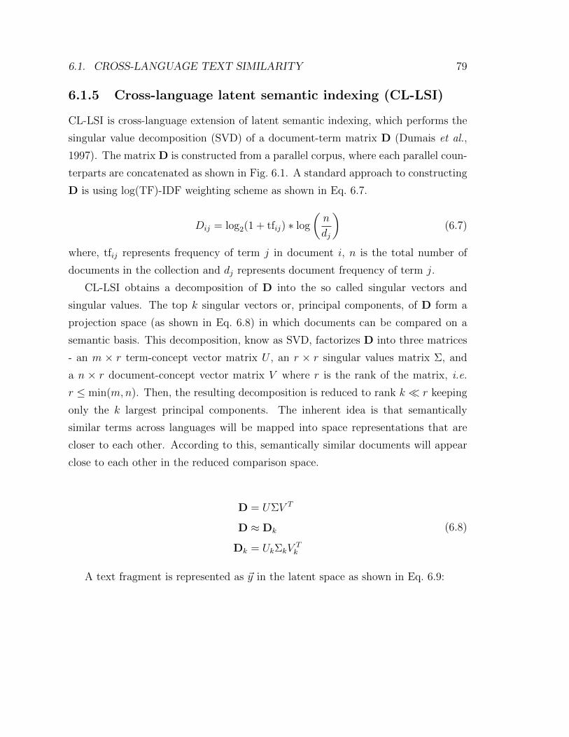
6.1. CROSS-LANGUAGE TEXT SIMILARITY 79
6.1.5 Cross-language latent semantic indexing (CL-LSI)
CL-LSI is cross-language extension of latent semantic indexing, which performs the
singular value decomposition (SVD) of a document-term matrix D (Dumais et al.,
1997). The matrix D is constructed from a parallel corpus, where each parallel coun-
terparts are concatenated as shown in Fig. 6.1. A standard approach to constructing
D is using log(TF)-IDF weighting scheme as shown in Eq. 6.7.
Dij = log2(1 + tfij) ∗ log
(n
dj
)(6.7)
where, tfij represents frequency of term j in document i, n is the total number of
documents in the collection and dj represents document frequency of term j.
CL-LSI obtains a decomposition of D into the so called singular vectors and
singular values. The top k singular vectors or, principal components, of D form a
projection space (as shown in Eq. 6.8) in which documents can be compared on a
semantic basis. This decomposition, know as SVD, factorizes D into three matrices
- an m × r term-concept vector matrix U , an r × r singular values matrix Σ, and
a n × r document-concept vector matrix V where r is the rank of the matrix, i.e.
r ≤ min(m,n). Then, the resulting decomposition is reduced to rank k � r keeping
only the k largest principal components. The inherent idea is that semantically
similar terms across languages will be mapped into space representations that are
closer to each other. According to this, semantically similar documents will appear
close to each other in the reduced comparison space.
D = UΣV T
D ≈ Dk
Dk = UkΣkVTk
(6.8)
A text fragment is represented as ~y in the latent space as shown in Eq. 6.9:
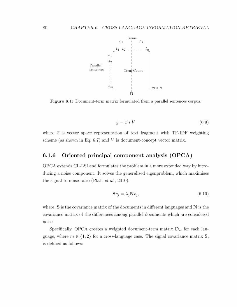
80 CHAPTER 6. CROSS-LANGUAGE INFORMATION RETRIEVAL
Terms
t1 t2 tns1s2
sm
Term Count
m x n
D
Parallelsentences
L1 L2
Figure 6.1: Document-term matrix formulated from a parallel sentences corpus.
~y = ~x ∗ V (6.9)
where ~x is vector space representation of text fragment with TF-IDF weighting
scheme (as shown in Eq. 6.7) and V is document-concept vector matrix.
6.1.6 Oriented principal component analysis (OPCA)
OPCA extends CL-LSI and formulates the problem in a more extended way by intro-
ducing a noise component. It solves the generalised eigenproblem, which maximises
the signal-to-noise ratio (Platt et al., 2010):
Svj = λjNvj, (6.10)
where, S is the covariance matrix of the documents in different languages and N is the
covariance matrix of the differences among parallel documents which are considered
noise.
Specifically, OPCA creates a weighted document-term matrix Dm for each lan-
guage, where m ∈ {1, 2} for a cross-language case. The signal covariance matrix S,
is defined as follows:
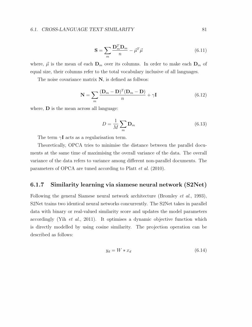
6.1. CROSS-LANGUAGE TEXT SIMILARITY 81
S =∑m
DTmDm
n− ~µT~µ (6.11)
where, ~µ is the mean of each Dm over its columns. In order to make each Dm of
equal size, their columns refer to the total vocabulary inclusive of all languages.
The noise covariance matrix N, is defined as follwos:
N =∑m
(Dm −D)T (Dm −D)
n+ γI (6.12)
where, D is the mean across all language:
D =1
M
∑m
Dm (6.13)
The term γI acts as a regularisation term.
Theoretically, OPCA tries to minimise the distance between the parallel docu-
ments at the same time of maximising the overall variance of the data. The overall
variance of the data refers to variance among different non-parallel documents. The
parameters of OPCA are tuned according to Platt et al. (2010).
6.1.7 Similarity learning via siamese neural network (S2Net)
Following the general Siamese neural network architecture (Bromley et al., 1993),
S2Net trains two identical neural networks concurrently. The S2Net takes in parallel
data with binary or real-valued similarity score and updates the model parameters
accordingly (Yih et al., 2011). It optimises a dynamic objective function which
is directly modelled by using cosine similarity. The projection operation can be
described as follows:
yd = W ∗ xd (6.14)
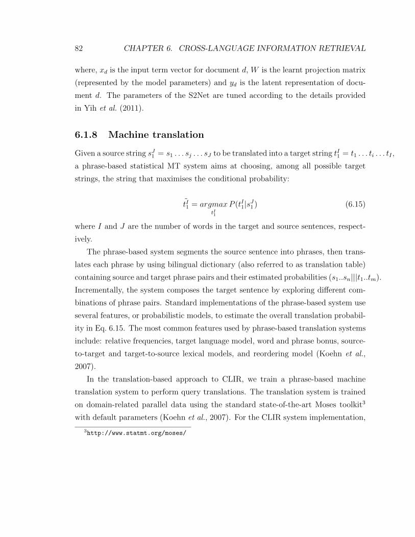
82 CHAPTER 6. CROSS-LANGUAGE INFORMATION RETRIEVAL
where, xd is the input term vector for document d, W is the learnt projection matrix
(represented by the model parameters) and yd is the latent representation of docu-
ment d. The parameters of the S2Net are tuned according to the details provided
in Yih et al. (2011).
6.1.8 Machine translation
Given a source string sJ1 = s1 . . . sj . . . sJ to be translated into a target string tI1 = t1 . . . ti . . . tI ,
a phrase-based statistical MT system aims at choosing, among all possible target
strings, the string that maximises the conditional probability:
tI1 = argmaxtI1
P (tI1|sJ1 ) (6.15)
where I and J are the number of words in the target and source sentences, respect-
ively.
The phrase-based system segments the source sentence into phrases, then trans-
lates each phrase by using bilingual dictionary (also referred to as translation table)
containing source and target phrase pairs and their estimated probabilities (s1..sn|||t1..tm).
Incrementally, the system composes the target sentence by exploring different com-
binations of phrase pairs. Standard implementations of the phrase-based system use
several features, or probabilistic models, to estimate the overall translation probabil-
ity in Eq. 6.15. The most common features used by phrase-based translation systems
include: relative frequencies, target language model, word and phrase bonus, source-
to-target and target-to-source lexical models, and reordering model (Koehn et al.,
2007).
In the translation-based approach to CLIR, we train a phrase-based machine
translation system to perform query translations. The translation system is trained
on domain-related parallel data using the standard state-of-the-art Moses toolkit3
with default parameters (Koehn et al., 2007). For the CLIR system implementation,
3http://www.statmt.org/moses/
6.1. CROSS-LANGUAGE TEXT SIMILARITY 83
the query is translated into the language of the document collection and then simil-
arity is calculated using the BM25 measure in a monolingual setting4. Although we
consider this system to be a baseline, we do not expect all cross-language latent ap-
proaches to necessarily outperform it, because this system operates in a monolingual
full-dimensional vector space in contrast to latent semantic models, which operate
in a cross-language low dimensional abstract space.
6.1.9 Hybrid models
The knowledge-based similarity analysis (KBSim) model (Franco-Salvador et al.,
2014) extends CL-KGA in order to combine the benefits of both, the knowledge
graph and the multilingual vector-based representations. Key to this approach is
the weighted combination of these two representations according to the relevance of
the knowledge graphs. This allows to increase the contribution of the multilingual
vector-based representations in case of non-informative knowledge graphs. Given a
source document d and a target document d′, we calculate the similarities between the
respective knowledge graphs and multilingual vector representations, and combine
the two resulting similarities to obtain a knowledge-based similarity as follows:
S(d, d′) = α ∗ Sg(G,G′) + (1− α) ∗ Sv(~v,~v
′), (6.16)
where Sg(G,G′) is the knowledge graph similarity of Eq. 6.6, Sv(~v,~v
′) is the vector-
based similarity, and α is an interpolation factor that is calculated as the edge density
of the knowledge graph G:
α =|E(G)|
|V(G)|(|V(G)| − 1)(6.17)
Note that, by using the factor α to interpolate the two similarities in Eq. 6.16,
the relative importance of each model is determined.
4We tried different retrieval models like BM25 and divergence from randomness based but thedifference in performance was not statistically significant
84 CHAPTER 6. CROSS-LANGUAGE INFORMATION RETRIEVAL
The vector-based similarity Sv(~v,~v′) computes the cosine similarity between vec-
tors in the continuous space. We adopt this framework to include information
provided by the continuous representation into similarity estimation. We evaluate the
performance of KBSim (S2Net), KBSim (CAE) and KBSim (XCNN) in Section 6.2.4
for cross-language plagiarism detection task.
6.1.10 Continuous word alignment-based similarity analysis
(CWASA)
The aforementioned models allow for learning a real-valued continuous space repres-
entation of texts. All of them combine basic word level representations by summing
over terms in order to model sequences of words. The method presented in this
section provides an alternative way to combine word level vectors by means of align-
ments to represent text. The continuous word alignment-based similarity analysis
model is based on the text-to-text relatedness proposed by (Hassan and Mihalcea,
2011). It estimates the similarity between documents by efficiently aligning their con-
tinuous word representations using directed edges. Formally, the similarity S(d, d′)
between two documents d and d′ is estimated as follows:
S(d, d′) =1
|Φ|∑ck∈Φ
ck, (6.18)
where d = (x1, ..., xn) and d′ = (y1, ..., ym) are represented as lists of continuous word
vectors, and Φ is generated from the list Φ′ = {c′1, ..., c′n+m} that satisfies Eq. 6.19:
c′k =
max
i=k,xi∈d,yj∈d′ϕ(xi, yj), if k ≤ n
maxj=k−n,xi∈d,yj∈d′
ϕ(xi, yj), otherwise(6.19)
where 1 ≤ i ≤ n, 1 ≤ j ≤ m, 1 ≤ k ≤ n+m, ϕ is the cosine similarity function, and
being Φ = {c1, ..., cz | max(n,m) ≤ z ≤ n+m}, Φ ⊆ Φ′, the set of cosine similarities
6.2. CROSS-LANGUAGE PLAGIARISM DETECTION 85
without pairing repetitions5 that represents the strongest semantic pairing between
the continuous word representations of documents d and d′.
Basically, in Eq. 6.19 each word in d is aligned with the closest one in d′ and vice
versa using directed relationships. Next, the duplicated alignments are removed, i.e.,
those equally aligned in both directions. Finally, the similarity score between d and
d′ is estimated by Eq. 6.18 as the average of the different alignments. More details
on CWASA can be found in (Franco-Salvador et al., 2016).
6.2 Cross-language plagiarism detection
Automatic plagiarism detection entails identifying plagiarised text fragments and
their corresponding original source. The task is defined in Sec. 6.2.1 and also pop-
ularly used in PAN6 track on plagiarism detection at CLEF (Potthast et al., 2009).
There have been many approaches to plagiarism detection (Potthast et al., 2009,
2010, 2011; Barron-Cedeno, 2012; Barron-Cedeno et al., 2013; Franco-Salvador et al.,
2013), but, as far as we know, latent semantic methods have not been explored for
this problem yet. We believe semantic similarity assessed by means of latent features
can provide a new interest approach to plagiarism detection.
6.2.1 Problem statement
Let dq be a suspicious document and D a set of potential source documents. The
core problem of plagiarism detection is to identify the set of all fragment pairs {sq, s}such that fragments sq ∈ dq have a high chance to be borrowed from fragments s ∈ d(with d ∈ D). After {sq, s} are identified, an expert can determine whether each
fragment pair is indeed a case of plagiarism (no proper citation is provided). From
a cross-language (CL) perspective, dq ∈ L and d′ ∈ L′, where L 6= L′, represent dif-
ferent languages. This problem is referred to as cross-language plagiarism detection
5The same pair of words are not allowed to be aligned twice.6http://pan.webis.de/
86 CHAPTER 6. CROSS-LANGUAGE INFORMATION RETRIEVAL
(CLPD).
We follow the general framework of cross-language plagiarism detection intro-
duced in Potthast et al. (2011). The process is divided into the three steps described
below:
(i) Candidate retrieval. A set of candidate documents D∗ is retrieved from D′
(with |D∗| � |D′|). D∗ contains the most similar documents to dq and, there-
fore, the most likely to contain potential cases of re-use.
(ii) Detailed analysis. dq is compared against every d′ ∈ D∗ section-wise. If a
pair {sq, s′} is identified to be more similar than expected for independently
generated texts, it is selected as a candidate of plagiarism.
(iii) Heuristic post-processing. Plagiarism candidates that are not long or do
not have similarity above a threshold are discarded. Additionally, heuristics
are applied to merge nearby candidates.7
Based on this framework, most of the research done on CL similarity estimation
is used for the candidate retrieval and detailed analysis steps, while heuristic post-
processing step mostly incorporates the domain knowledge for the CLPD task.
6.2.2 Detailed analysis method
The step of identifying plagiarised sections in suspicious document dq from source
document d′ is referred to as detailed analysis. A framework for detailed analysis is
presented in Algorithm 2 which is also a contribution of this work (Barron-Cedeno
et al., 2013). In the detailed analysis, dq and d′ are split into chunks of certain length
w and step size t. We select w = 5 and t = 2 sentences aiming at considering chunks
close to paragraphs (Barron-Cedeno et al., 2013); sim(sq, s′) computes the similarity
between the text fragments based on a similarity estimation algorithm discussed
7This step had been originally intended to filter false positives, such as cases of borrowing withproper citation (Stein et al., 2007).
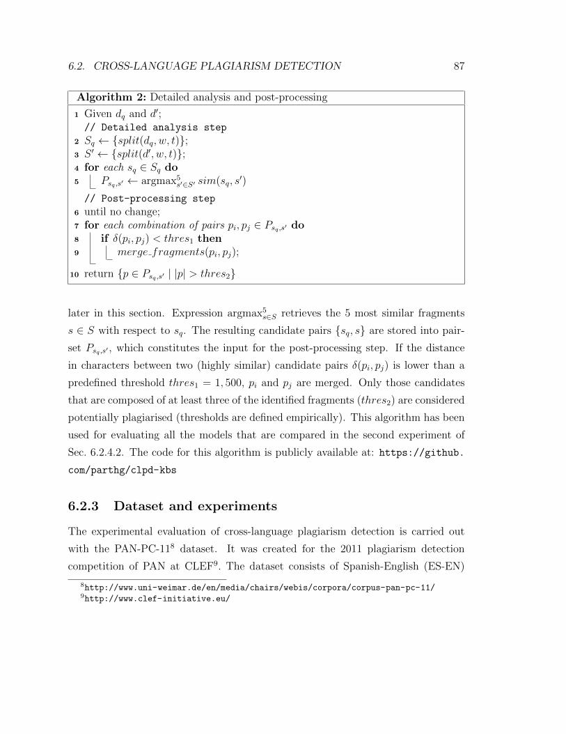
6.2. CROSS-LANGUAGE PLAGIARISM DETECTION 87
Algorithm 2: Detailed analysis and post-processing
1 Given dq and d′;// Detailed analysis step
2 Sq ← {split(dq, w, t)};3 S ′ ← {split(d′, w, t)};4 for each sq ∈ Sq do5 Psq ,s′ ← argmax5
s′∈S′ sim(sq, s′)
// Post-processing step
6 until no change;7 for each combination of pairs pi, pj ∈ Psq ,s′ do8 if δ(pi, pj) < thres1 then9 merge fragments(pi, pj);
10 return {p ∈ Psq ,s′ | |p| > thres2}
later in this section. Expression argmax5s∈S retrieves the 5 most similar fragments
s ∈ S with respect to sq. The resulting candidate pairs {sq, s} are stored into pair-
set Psq ,s′ , which constitutes the input for the post-processing step. If the distance
in characters between two (highly similar) candidate pairs δ(pi, pj) is lower than a
predefined threshold thres1 = 1, 500, pi and pj are merged. Only those candidates
that are composed of at least three of the identified fragments (thres2) are considered
potentially plagiarised (thresholds are defined empirically). This algorithm has been
used for evaluating all the models that are compared in the second experiment of
Sec. 6.2.4.2. The code for this algorithm is publicly available at: https://github.
com/parthg/clpd-kbs
6.2.3 Dataset and experiments
The experimental evaluation of cross-language plagiarism detection is carried out
with the PAN-PC-118 dataset. It was created for the 2011 plagiarism detection
competition of PAN at CLEF9. The dataset consists of Spanish-English (ES-EN)
8http://www.uni-weimar.de/en/media/chairs/webis/corpora/corpus-pan-pc-11/9http://www.clef-initiative.eu/
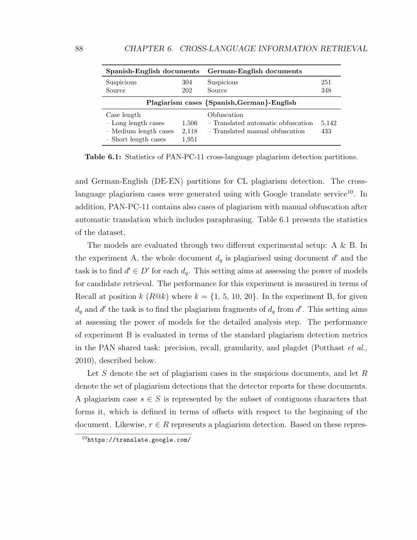
88 CHAPTER 6. CROSS-LANGUAGE INFORMATION RETRIEVAL
Spanish-English documents German-English documents
Suspicious 304 Suspicious 251Source 202 Source 348
Plagiarism cases {Spanish,German}-English
Case length Obfuscation– Long length cases 1,506 – Translated automatic obfuscation 5,142– Medium length cases 2,118 – Translated manual obfuscation 433– Short length cases 1,951
Table 6.1: Statistics of PAN-PC-11 cross-language plagiarism detection partitions.
and German-English (DE-EN) partitions for CL plagiarism detection. The cross-
language plagiarism cases were generated using with Google translate service10. In
addition, PAN-PC-11 contains also cases of plagiarism with manual obfuscation after
automatic translation which includes paraphrasing. Table 6.1 presents the statistics
of the dataset.
The models are evaluated through two different experimental setup: A & B. In
the experiment A, the whole document dq is plagiarised using document d′ and the
task is to find d′ ∈ D′ for each dq. This setting aims at assessing the power of models
for candidate retrieval. The performance for this experiment is measured in terms of
Recall at position k (R@k) where k = {1, 5, 10, 20}. In the experiment B, for given
dq and d′ the task is to find the plagiarism fragments of dq from d′. This setting aims
at assessing the power of models for the detailed analysis step. The performance
of experiment B is evaluated in terms of the standard plagiarism detection metrics
in the PAN shared task: precision, recall, granularity, and plagdet (Potthast et al.,
2010), described below.
Let S denote the set of plagiarism cases in the suspicious documents, and let R
denote the set of plagiarism detections that the detector reports for these documents.
A plagiarism case s ∈ S is represented by the subset of contiguous characters that
forms it, which is defined in terms of offsets with respect to the beginning of the
document. Likewise, r ∈ R represents a plagiarism detection. Based on these repres-
10https://translate.google.com/
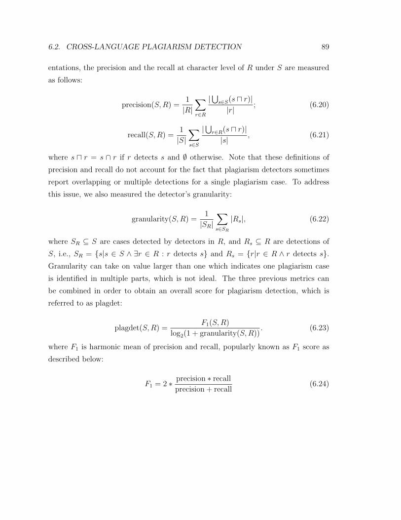
6.2. CROSS-LANGUAGE PLAGIARISM DETECTION 89
entations, the precision and the recall at character level of R under S are measured
as follows:
precision(S,R) =1
|R|∑r∈R
|⋃s∈S(s u r)||r| ; (6.20)
recall(S,R) =1
|S|∑s∈S
|⋃r∈R(s u r)||s| , (6.21)
where s u r = s ∩ r if r detects s and ∅ otherwise. Note that these definitions of
precision and recall do not account for the fact that plagiarism detectors sometimes
report overlapping or multiple detections for a single plagiarism case. To address
this issue, we also measured the detector’s granularity:
granularity(S,R) =1
|SR|∑s∈SR
|Rs|, (6.22)
where SR ⊆ S are cases detected by detectors in R, and Rs ⊆ R are detections of
S, i.e., SR = {s|s ∈ S ∧ ∃r ∈ R : r detects s} and Rs = {r|r ∈ R ∧ r detects s}.Granularity can take on value larger than one which indicates one plagiarism case
is identified in multiple parts, which is not ideal. The three previous metrics can
be combined in order to obtain an overall score for plagiarism detection, which is
referred to as plagdet:
plagdet(S,R) =F1(S,R)
log2(1 + granularity(S,R)). (6.23)
where F1 is harmonic mean of precision and recall, popularly known as F1 score as
described below:
F1 = 2 ∗ precision ∗ recall
precision + recall(6.24)
90 CHAPTER 6. CROSS-LANGUAGE INFORMATION RETRIEVAL
6.2.4 Results and analysis
In this section we present the results and the corresponding analysis for the exper-
imental evaluation on cross-language plagiarism detection. First, details on specific
experimental settings for each model are presented, followed by the experiments and
their corresponding results.
(i) CL-C3G It is CL-CNG using character 3-grams, as recommended in Potthast
et al. (2011).
(ii) CL-ESA We used 10,000 Spanish-German-English comparable Wikipedia pages
as document collection. All pages contain more than 10,000 characters and were rep-
resented using TF-IDF weighting. The similarities are computed using the cosine
similarity and the IDF of the words is calculated from the complete Wikipedia in
each language.
(iii) CL-ASA We used a statistical dictionary trained using the word-alignment
model IBM-1 (Och and Ney, 2003) on the JRC-Acquis corpus (Steinberger et al.,
2006).
(iv) CL-KGA We used the multilingual semantic network BabelNet (Navigli and
Ponzetto, 2012) to construct the graph and parameter tuning is as per (Franco-
Salvador et al., 2013).
(v) S2Net, CAE, XCNN We trained these models as described in Section 6.3.2.
We present experimental results for each of these models alone and in two differ-
ent settings: (i) when CWASA composition model is applied on embeddings learnt
through continuous models; and (ii) hybrid models using the KBSim framework.
For the readability and ease of comparison of the results, the models are grouped
according to their category: (a) vector space approaches, (b) continuous space mod-
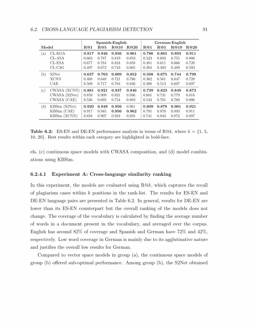
6.2. CROSS-LANGUAGE PLAGIARISM DETECTION 91
Spanish-English German-EnglishModel R@1 R@5 R@10 R@20 R@1 R@5 R@10 R@20
(a) CL-KGA 0.917 0.946 0.956 0.961 0.786 0.865 0.893 0.911CL-ASA 0.663 0.787 0.819 0.853 0.523 0.693 0.755 0.806CL-ESA 0.677 0.784 0.824 0.858 0.481 0.611 0.666 0.720CL-C3G 0.497 0.672 0.743 0.805 0.204 0.393 0.489 0.593
(b) S2Net 0.637 0.763 0.809 0.852 0.508 0.675 0.744 0.799XCNN 0.468 0.648 0.721 0.786 0.362 0.561 0.647 0.728CAE 0.509 0.717 0.784 0.836 0.308 0.513 0.607 0.697
(c) CWASA (XCNN) 0.881 0.921 0.937 0.946 0.739 0.823 0.849 0.873CWASA (S2Net) 0.859 0.909 0.921 0.936 0.601 0.731 0.779 0.818CWASA (CAE) 0.536 0.695 0.754 0.803 0.543 0.701 0.760 0.806
(d) KBSim (S2Net) 0.920 0.949 0.956 0.961 0.809 0.878 0.901 0.921KBSim (CAE) 0.917 0.945 0.956 0.962 0.791 0.870 0.893 0.911KBSim (XCNN) 0.858 0.907 0.924 0.935 0.741 0.843 0.872 0.897
Table 6.2: ES-EN and DE-EN performance analysis in terms of R@k , where k = {1, 5,10, 20}. Best results within each category are highlighted in bold-face.
els, (c) continuous space models with CWASA composition, and (d) model combin-
ations using KBSim.
6.2.4.1 Experiment A: Cross-language similarity ranking
In this experiment, the models are evaluated using R@k , which captures the recall
of plagiarism cases within k positions in the rank-list. The results for ES-EN and
DE-EN language pairs are presented in Table 6.2. In general, results for DE-EN are
lower than its ES-EN counterpart but the overall ranking of the models does not
change. The coverage of the vocabulary is calculated by finding the average number
of words in a document present in the vocabulary, and averaged over the corpus.
English has around 82% of coverage and Spanish and German have 72% and 42%,
respectively. Low word coverage in German is mainly due to its agglutinative nature
and justifies the overall low results for German.
Compared to vector space models in group (a), the continuous space models of
group (b) offered sub-optimal performance. Among group (b), the S2Net obtained
92 CHAPTER 6. CROSS-LANGUAGE INFORMATION RETRIEVAL
the best results. It should be noted that S2Net and CAE directly learn representa-
tions of text using the bag-of-words approach. In contrast, XCNN learns word-level
embeddings and hence when modeling documents, which are large fragments of text
(∼1000 words), the summation of such a large number of word-level representations
affects the discriminative power of the model, affecting XCNN performance. The
advantages of XCNN will be more clear in Experiment B, where the fragments being
compared are small and this effect is less severe.
The use of a different composition method with continuous representation, such
as CWASA, boosts the performance of all continuous space models. Particularly,
XCNN benefits the most and becomes the best performing model in the correspond-
ing category (c). This also reaffirms the fact that XCNN can learn discriminative
representations. However, the simple addition of word-level representations limits
its full potential, especially when the text fragment is large. It should also be noted
that CWASA (XCNN) is not comparable to CL-KGA. While the former is trained
on a limited parallel corpus and operates on 20k dimensional vocabulary, CL-KGA
leverages on a large sophisticated multilingual resource such as BabelNet with more
than 9M concepts.
The hybrid models in group (d) which combine knowledge graphs and continuous
space models, produce the best results; even outperforming a strong model such as
CL-KGA. This gives evidence that continuous space models are a good complement
to discrete models. The high performance of these models suggests that latent se-
mantic models provide powerful features for the candidate retrieval task of plagiarism
detection.
6.2.4.2 Experiment B: Cross-language plagiarism detection
This second experiment aims at evaluating the detection of plagiarism cases at the
fragment level. Different cross-language similarity estimation models are used in
Algorithm 2 for fragment identification. The performance is evaluated on stand-
ard metrics for plagiarism detection task, such as precision, recall, granularity and
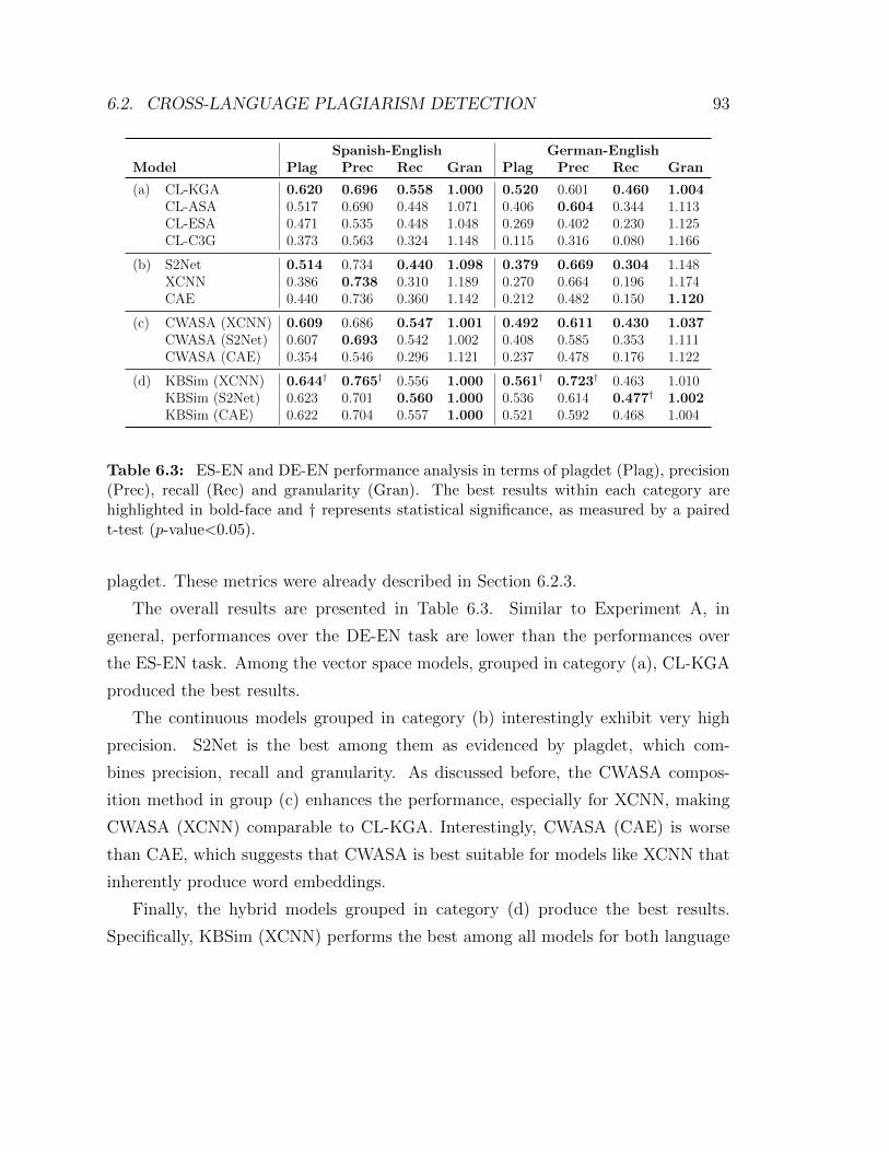
6.2. CROSS-LANGUAGE PLAGIARISM DETECTION 93
Spanish-English German-EnglishModel Plag Prec Rec Gran Plag Prec Rec Gran
(a) CL-KGA 0.620 0.696 0.558 1.000 0.520 0.601 0.460 1.004CL-ASA 0.517 0.690 0.448 1.071 0.406 0.604 0.344 1.113CL-ESA 0.471 0.535 0.448 1.048 0.269 0.402 0.230 1.125CL-C3G 0.373 0.563 0.324 1.148 0.115 0.316 0.080 1.166
(b) S2Net 0.514 0.734 0.440 1.098 0.379 0.669 0.304 1.148XCNN 0.386 0.738 0.310 1.189 0.270 0.664 0.196 1.174CAE 0.440 0.736 0.360 1.142 0.212 0.482 0.150 1.120
(c) CWASA (XCNN) 0.609 0.686 0.547 1.001 0.492 0.611 0.430 1.037CWASA (S2Net) 0.607 0.693 0.542 1.002 0.408 0.585 0.353 1.111CWASA (CAE) 0.354 0.546 0.296 1.121 0.237 0.478 0.176 1.122
(d) KBSim (XCNN) 0.644† 0.765† 0.556 1.000 0.561† 0.723† 0.463 1.010KBSim (S2Net) 0.623 0.701 0.560 1.000 0.536 0.614 0.477† 1.002KBSim (CAE) 0.622 0.704 0.557 1.000 0.521 0.592 0.468 1.004
Table 6.3: ES-EN and DE-EN performance analysis in terms of plagdet (Plag), precision(Prec), recall (Rec) and granularity (Gran). The best results within each category arehighlighted in bold-face and † represents statistical significance, as measured by a pairedt-test (p-value<0.05).
plagdet. These metrics were already described in Section 6.2.3.
The overall results are presented in Table 6.3. Similar to Experiment A, in
general, performances over the DE-EN task are lower than the performances over
the ES-EN task. Among the vector space models, grouped in category (a), CL-KGA
produced the best results.
The continuous models grouped in category (b) interestingly exhibit very high
precision. S2Net is the best among them as evidenced by plagdet, which com-
bines precision, recall and granularity. As discussed before, the CWASA compos-
ition method in group (c) enhances the performance, especially for XCNN, making
CWASA (XCNN) comparable to CL-KGA. Interestingly, CWASA (CAE) is worse
than CAE, which suggests that CWASA is best suitable for models like XCNN that
inherently produce word embeddings.
Finally, the hybrid models grouped in category (d) produce the best results.
Specifically, KBSim (XCNN) performs the best among all models for both language
94 CHAPTER 6. CROSS-LANGUAGE INFORMATION RETRIEVAL
pairs. This observation (similar to the corresponding one in Experiment A) confirms
that knowledge graphs and continuous space models capture different aspects of text
and complement each other.
6.3 Cross-language ad-hoc retrieval
Cross-language ad-hoc retrieval addresses the situation where a system is presented
with an information need in form of a few keywords. The system has to produce a
ranked list of documents that are relevant to the provided information need. The
CAE and XCNN models are evaluated on the standard ad-hoc retrieval task in the
cross-language setting. Current search engines do not employ CLIR systems for web
search because of several user-experience aspects such as presentation of results and
query formulation. The most suitable use-cases are the following:
1. A bilingual user issuing a query in one language and assessing the results in a
different language, where the relevant information is only available in the latter
language.
2. A mono-lingual user issuing a query in one language and assessing results in
the same language with the help of automatic translation systems, where the
relevant information is only available in a different language.
An example of these scenarios are: a Spaniard with a limited knowledge of Eng-
lish, who visits U.K. and formulates a query in Spanish; or a Briton (who only knows
English) who visits Spain and formulates a query in English. In case the user is not
acquainted with the language of the retrieved documents, an automatic machine
translation system can be used to present results in the language of user preference.
6.3.1 Problem statement
Let D denote a collection of documents in language L1 and information need is
expressed by query q in language L2. The task is to generate a ranked list (R) of
6.3. CROSS-LANGUAGE AD-HOC RETRIEVAL 95
documents from D in decreasing order of relevance.
6.3.2 Methods
There are two main approaches to cross-language information retrieval: (i) machine-
translation, and (ii) cross-language latent semantic projections. In machine trans-
lation based approaches, an MT system from L2 → L1 is used to represent query q
in L1, and then, mono-lingual IR is carried out. In latent semantic projection based
approaches, a cross-language projection function is used to represent both D ∈ L1
and q ∈ L2 in a low-dimensional abstract, where semantic similarity is estimated.
6.3.3 Datasets and experiments
Our CLIR experimental evaluation is carried out on the FIRE 2011-12 En-Hi CLIR
track corpus11. It contains 100 English queries (topics), 331,599 news articles in
Hindi and their corresponding relevance judgments (qrels). The corpus contains
news articles that cover different domains including entertainment, politics, busi-
ness, popular culture etc. The topics are formulated by browsing the corpus and
refined further based on initial retrieval results to ensure the minimum number of
relevant documents per query. This is to make a balance between easy, medium and
hard queries. The collection contains binary relevance judgments generated through
a pool of submitted runs (Palchowdhury et al., 2011). The retrieval results are eval-
uated by the standard IR metrics, more specifically, we used mean reciprocal rank
(MRR), mean average-precision (MAP) and normalised discounted cumulative gain
(nDCG) (Jarvelin and Kekalainen, 2002). MRR is described in Eq. 6.25 and nDCG
is described in Sec. 2.1.3.
MRR =1
|Q|
|Q|∑i=1
1
ranki(6.25)
11http://www.isical.ac.in/~fire/
96 CHAPTER 6. CROSS-LANGUAGE INFORMATION RETRIEVAL
where Q is the query-set and ranki is the rank of the first relevant document for
query i.
For training the latent semantic models and the MT system, the En-Hi parallel
corpus available from WMT 201412 (Bojar et al., 2014b) was used. In total, 100k
parallel sentences from the corpus were used, which at least contained 3 terms from
the selected vocabulary. The selected vocabulary consisted of 20k (10+10) most
frequent terms, which were selected after removing stopwords. A stemmer is used
applied to represent text.
6.3.4 Results and analysis
Here, we present the results and analysis of XCNN for the task of cross-language ad-
hoc retrieval (Gupta et al., 2016a). In order to step-by-step analyse XCNN learning,
the monolingual pre-initialisation is evaluated first, because that makes the basis for
the cross-language extension. We compare its performance with a standard BM25
baseline to ensure reliability of the model, referred as mono-XCNN. At this stage
mono-XCNN is not expected to outperform the vector space model because the final
objective of the model is to learn cross-language associations. Naturally, the FIRE
collection does not provide click-through data. In absence of click-through data,
we use pseudo-relevance data as positive samples for training data. Concretely, the
sentence with the highest BM25 score w.r.t. the input sentence is chosen as positive
sample for it. The document collection is in Hindi, hence we report results with Hindi
queries in monolingual setting. The code for the XCNN model is publicly available
at: https://github.com/parthg/jDNN
The results using Hindi queries are presented in Table 6.4. In the table, BM25
and mono-XCNN are evaluated using a limited vocabulary of size 10k. Interestingly,
for the top rank-position related metrics like nDCG@1 and MRR, mono-XCNN per-
forms better than BM25. For other metrics which involve lower rank positions, the
performance of mono-XCNN is sub-optimal to the VSM approach. This is not sur-
12ACL 2014 ninth workshop on statistical machine translation http://www.statmt.org/wmt14/.
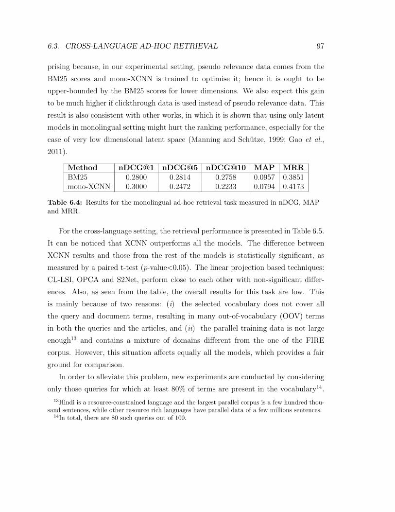
6.3. CROSS-LANGUAGE AD-HOC RETRIEVAL 97
prising because, in our experimental setting, pseudo relevance data comes from the
BM25 scores and mono-XCNN is trained to optimise it; hence it is ought to be
upper-bounded by the BM25 scores for lower dimensions. We also expect this gain
to be much higher if clickthrough data is used instead of pseudo relevance data. This
result is also consistent with other works, in which it is shown that using only latent
models in monolingual setting might hurt the ranking performance, especially for the
case of very low dimensional latent space (Manning and Schutze, 1999; Gao et al.,
2011).
Method nDCG@1 nDCG@5 nDCG@10 MAP MRRBM25 0.2800 0.2814 0.2758 0.0957 0.3851mono-XCNN 0.3000 0.2472 0.2233 0.0794 0.4173
Table 6.4: Results for the monolingual ad-hoc retrieval task measured in nDCG, MAPand MRR.
For the cross-language setting, the retrieval performance is presented in Table 6.5.
It can be noticed that XCNN outperforms all the models. The difference between
XCNN results and those from the rest of the models is statistically significant, as
measured by a paired t-test (p-value<0.05). The linear projection based techniques:
CL-LSI, OPCA and S2Net, perform close to each other with non-significant differ-
ences. Also, as seen from the table, the overall results for this task are low. This
is mainly because of two reasons: (i) the selected vocabulary does not cover all
the query and document terms, resulting in many out-of-vocabulary (OOV) terms
in both the queries and the articles, and (ii) the parallel training data is not large
enough13 and contains a mixture of domains different from the one of the FIRE
corpus. However, this situation affects equally all the models, which provides a fair
ground for comparison.
In order to alleviate this problem, new experiments are conducted by considering
only those queries for which at least 80% of terms are present in the vocabulary14.
13Hindi is a resource-constrained language and the largest parallel corpus is a few hundred thou-sand sentences, while other resource rich languages have parallel data of a few millions sentences.
14In total, there are 80 such queries out of 100.
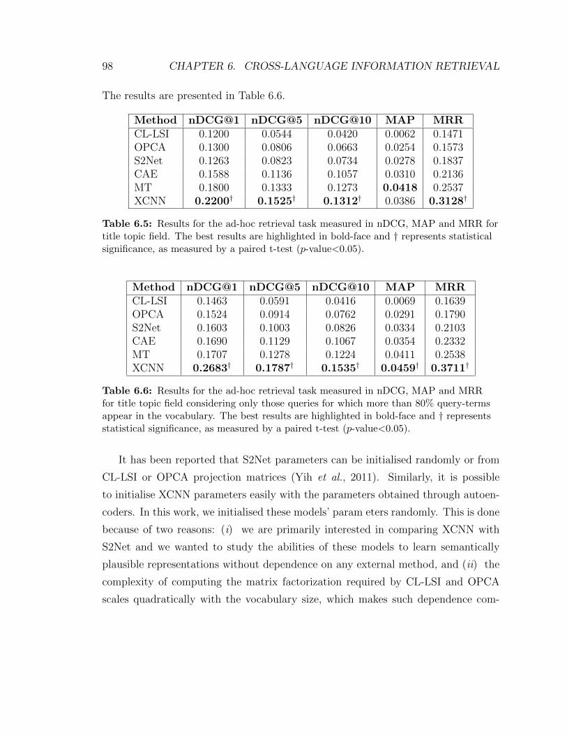
98 CHAPTER 6. CROSS-LANGUAGE INFORMATION RETRIEVAL
The results are presented in Table 6.6.
Method nDCG@1 nDCG@5 nDCG@10 MAP MRRCL-LSI 0.1200 0.0544 0.0420 0.0062 0.1471OPCA 0.1300 0.0806 0.0663 0.0254 0.1573S2Net 0.1263 0.0823 0.0734 0.0278 0.1837CAE 0.1588 0.1136 0.1057 0.0310 0.2136MT 0.1800 0.1333 0.1273 0.0418 0.2537XCNN 0.2200† 0.1525† 0.1312† 0.0386 0.3128†
Table 6.5: Results for the ad-hoc retrieval task measured in nDCG, MAP and MRR fortitle topic field. The best results are highlighted in bold-face and † represents statisticalsignificance, as measured by a paired t-test (p-value<0.05).
Method nDCG@1 nDCG@5 nDCG@10 MAP MRRCL-LSI 0.1463 0.0591 0.0416 0.0069 0.1639OPCA 0.1524 0.0914 0.0762 0.0291 0.1790S2Net 0.1603 0.1003 0.0826 0.0334 0.2103CAE 0.1690 0.1129 0.1067 0.0354 0.2332MT 0.1707 0.1278 0.1224 0.0411 0.2538XCNN 0.2683† 0.1787† 0.1535† 0.0459† 0.3711†
Table 6.6: Results for the ad-hoc retrieval task measured in nDCG, MAP and MRRfor title topic field considering only those queries for which more than 80% query-termsappear in the vocabulary. The best results are highlighted in bold-face and † representsstatistical significance, as measured by a paired t-test (p-value<0.05).
It has been reported that S2Net parameters can be initialised randomly or from
CL-LSI or OPCA projection matrices (Yih et al., 2011). Similarly, it is possible
to initialise XCNN parameters easily with the parameters obtained through autoen-
coders. In this work, we initialised these models’ param eters randomly. This is done
because of two reasons: (i) we are primarily interested in comparing XCNN with
S2Net and we wanted to study the abilities of these models to learn semantically
plausible representations without dependence on any external method, and (ii) the
complexity of computing the matrix factorization required by CL-LSI and OPCA
scales quadratically with the vocabulary size, which makes such dependence com-
6.4. CROSS-LANGUAGE PARALLEL SENTENCE RETRIEVAL 99
putationally impractical for high dimensional applications such as ad-hoc retrieval.
Interestingly, as seen in the tables, XCNN is also able to outperform the MT based
method. This confirms that XCNN is able to capture useful cross-language semantic
representations within a very low dimensional space.
6.4 Cross-language parallel sentence retrieval
With the advent of the web, cross-language information retrieval becomes important
not only to satisfy the information need across languages but to mine resources across
multiple languages, such as for example parallel or comparable documents. Such
mined resources aid training machine translation systems (Munteanu and Marcu,
2005; Ture and Lin, 2012). In this sense, the aim of cross-language parallel sentence
retrieval is to find parallel counterparts across different languages for a given sentence,
or text fragment.
6.4.1 Problem statement
Let S denote a collection of sentences in language L1 and q, an input sentence in
language L2. The task of parallel sentence retrieval is to find potential translations
for input sentence q in S.
6.4.2 Datasets and experiments
The En-Hi parallel corpus available from WMT 201415 is used for training and evalu-
ation. The parallel sentences come from various sources like news articles, comment-
aries, Wikipedia, TED talks etc. More details on the corpus is available in Bojar
et al. (2014b). The corpus contains a total of 274k parallel sentences. The working
vocabulary was extracted by removing stopwords, applying stemming and keeping
the most frequent 20k words (10k for each language). Finally, 122k parallel sentences,
15ACL 2014 ninth workshop on statistical machine translation http://www.statmt.org/wmt14/.
100 CHAPTER 6. CROSS-LANGUAGE INFORMATION RETRIEVAL
which at least contained 3 terms from the vocabulary, were used for training (100k)
and evaluation (the remaining 22k).16 For a fair comparison, all the models were
trained and evaluated over the same training and evaluation partitions and with the
same vocabulary.
6.4.3 Results and analysis
The results for the sentence retrieval task are presented in Table 6.7. The retrieval
quality for each test sentence is assessed by considering its parallel counterpart’s
reciprocal rank in the rank-list. For this, we have used the MRR as evaluation
metric.
In general, the models including a noise-contrastive component outperform the
ones without it; e.g. OPCA vs. CL-LSI, and {XCNN, S2Net} vs. CAE. It suggests
that having such component lead to better representation learning. It should also be
noted that models such as S2Net and XCNN, which directly optimise the evaluation
metric (cosine similarity) outperform the rest of latent space models such as CL-LSI,
OPCA and CAE. It can be noticed from Table 6.7, that the proposed method clearly
outperforms the other methods. Moreover, the observed difference is statistically
significant (p-value less than 0.01) according to the paired t-test. It should also be
noted that each non-linear model outperforms its corresponding linear counterparts;
e.g. CAE vs. {CL-LSI, OPCA}, and XCNN vs. S2Net.
6.5 Source context for machine translation
In this section, we present the problem of lexical selection in machine translation.
Such problem is handled with source context features. First, we describe the source
context features and then show how the continuous space model CAE (c.f. Sec. 4.1)
is used to provide such feature (Gupta et al., 2016b).
Source context is usually very relevant when translating texts. However, standard
16Many sentences were just one word being named entities extracted from Wikipedia page titles.
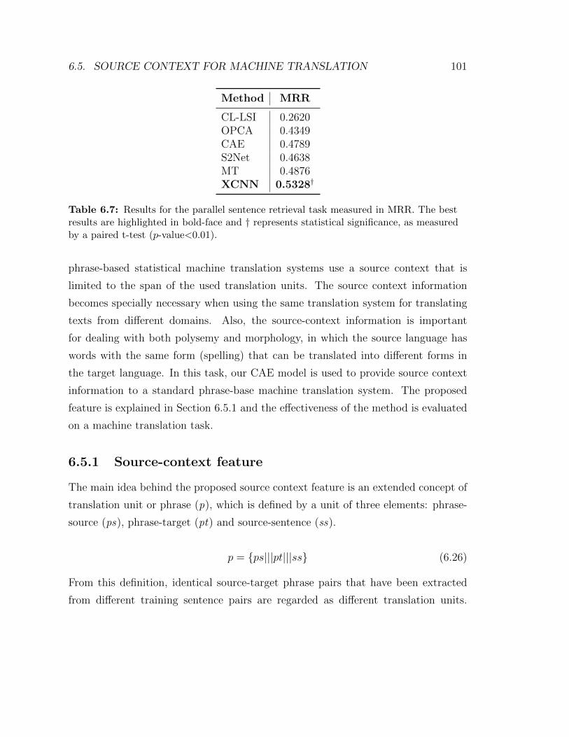
6.5. SOURCE CONTEXT FOR MACHINE TRANSLATION 101
Method MRR
CL-LSI 0.2620OPCA 0.4349CAE 0.4789S2Net 0.4638MT 0.4876XCNN 0.5328†
Table 6.7: Results for the parallel sentence retrieval task measured in MRR. The bestresults are highlighted in bold-face and † represents statistical significance, as measuredby a paired t-test (p-value<0.01).
phrase-based statistical machine translation systems use a source context that is
limited to the span of the used translation units. The source context information
becomes specially necessary when using the same translation system for translating
texts from different domains. Also, the source-context information is important
for dealing with both polysemy and morphology, in which the source language has
words with the same form (spelling) that can be translated into different forms in
the target language. In this task, our CAE model is used to provide source context
information to a standard phrase-base machine translation system. The proposed
feature is explained in Section 6.5.1 and the effectiveness of the method is evaluated
on a machine translation task.
6.5.1 Source-context feature
The main idea behind the proposed source context feature is an extended concept of
translation unit or phrase (p), which is defined by a unit of three elements: phrase-
source (ps), phrase-target (pt) and source-sentence (ss).
p = {ps|||pt|||ss} (6.26)
From this definition, identical source-target phrase pairs that have been extracted
from different training sentence pairs are regarded as different translation units.
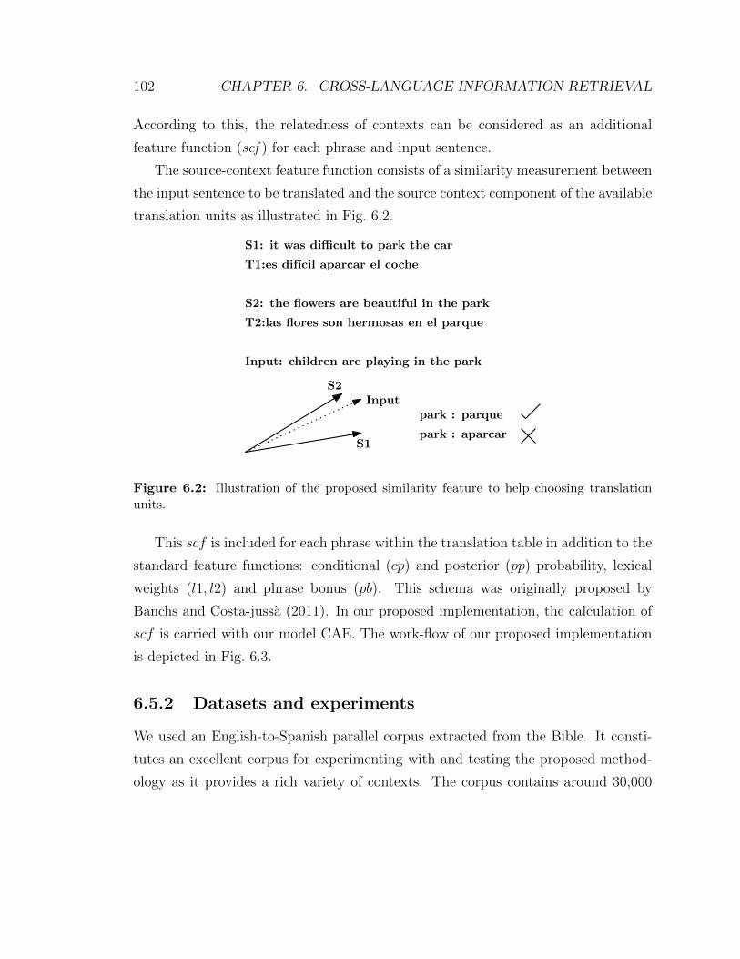
102 CHAPTER 6. CROSS-LANGUAGE INFORMATION RETRIEVAL
According to this, the relatedness of contexts can be considered as an additional
feature function (scf ) for each phrase and input sentence.
The source-context feature function consists of a similarity measurement between
the input sentence to be translated and the source context component of the available
translation units as illustrated in Fig. 6.2.
S1: it was difficult to park the car
T1:es difıcil aparcar el coche
S2: the flowers are beautiful in the park
T2:las flores son hermosas en el parque
Input: children are playing in the park
park : parque
park : aparcar
S2
S1
Input
Figure 6.2: Illustration of the proposed similarity feature to help choosing translationunits.
This scf is included for each phrase within the translation table in addition to the
standard feature functions: conditional (cp) and posterior (pp) probability, lexical
weights (l1, l2) and phrase bonus (pb). This schema was originally proposed by
Banchs and Costa-jussa (2011). In our proposed implementation, the calculation of
scf is carried with our model CAE. The work-flow of our proposed implementation
is depicted in Fig. 6.3.
6.5.2 Datasets and experiments
We used an English-to-Spanish parallel corpus extracted from the Bible. It consti-
tutes an excellent corpus for experimenting with and testing the proposed method-
ology as it provides a rich variety of contexts. The corpus contains around 30,000
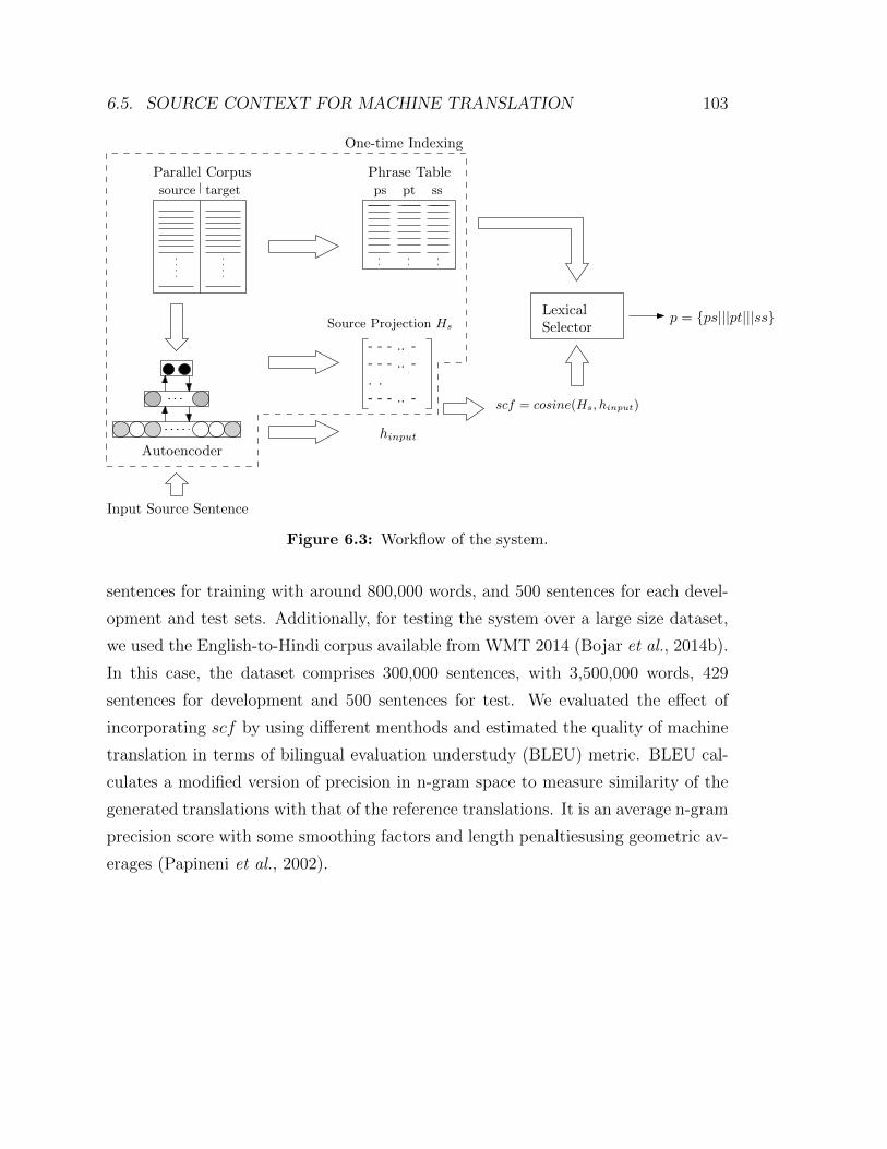
6.5. SOURCE CONTEXT FOR MACHINE TRANSLATION 103
source target
Autoencoder
Parallel Corpus Phrase Table
LexicalSelector
- - - .. -- - - .. -. .- - - .. -
Input Source Sentence
p = {ps|||pt|||ss}
ps pt ss
Source Projection Hs
hinput
scf = cosine(Hs, hinput)
One-time Indexing
Figure 6.3: Workflow of the system.
sentences for training with around 800,000 words, and 500 sentences for each devel-
opment and test sets. Additionally, for testing the system over a large size dataset,
we used the English-to-Hindi corpus available from WMT 2014 (Bojar et al., 2014b).
In this case, the dataset comprises 300,000 sentences, with 3,500,000 words, 429
sentences for development and 500 sentences for test. We evaluated the effect of
incorporating scf by using different menthods and estimated the quality of machine
translation in terms of bilingual evaluation understudy (BLEU) metric. BLEU cal-
culates a modified version of precision in n-gram space to measure similarity of the
generated translations with that of the reference translations. It is an average n-gram
precision score with some smoothing factors and length penaltiesusing geometric av-
erages (Papineni et al., 2002).
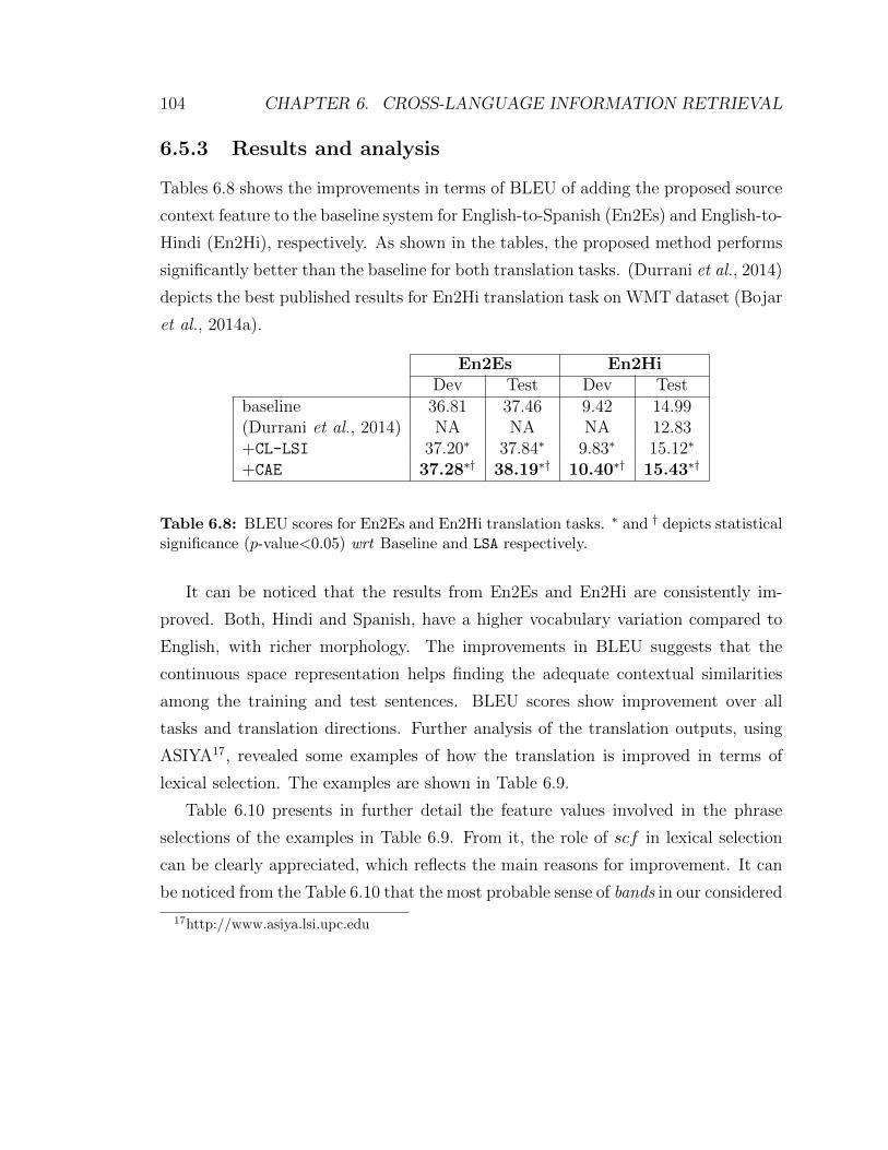
104 CHAPTER 6. CROSS-LANGUAGE INFORMATION RETRIEVAL
6.5.3 Results and analysis
Tables 6.8 shows the improvements in terms of BLEU of adding the proposed source
context feature to the baseline system for English-to-Spanish (En2Es) and English-to-
Hindi (En2Hi), respectively. As shown in the tables, the proposed method performs
significantly better than the baseline for both translation tasks. (Durrani et al., 2014)
depicts the best published results for En2Hi translation task on WMT dataset (Bojar
et al., 2014a).
En2Es En2HiDev Test Dev Test
baseline 36.81 37.46 9.42 14.99(Durrani et al., 2014) NA NA NA 12.83+CL-LSI 37.20∗ 37.84∗ 9.83∗ 15.12∗
+CAE 37.28∗† 38.19∗† 10.40∗† 15.43∗†
Table 6.8: BLEU scores for En2Es and En2Hi translation tasks. ∗ and † depicts statisticalsignificance (p-value<0.05) wrt Baseline and LSA respectively.
It can be noticed that the results from En2Es and En2Hi are consistently im-
proved. Both, Hindi and Spanish, have a higher vocabulary variation compared to
English, with richer morphology. The improvements in BLEU suggests that the
continuous space representation helps finding the adequate contextual similarities
among the training and test sentences. BLEU scores show improvement over all
tasks and translation directions. Further analysis of the translation outputs, using
ASIYA17, revealed some examples of how the translation is improved in terms of
lexical selection. The examples are shown in Table 6.9.
Table 6.10 presents in further detail the feature values involved in the phrase
selections of the examples in Table 6.9. From it, the role of scf in lexical selection
can be clearly appreciated, which reflects the main reasons for improvement. It can
be noticed from the Table 6.10 that the most probable sense of bands in our considered
17http://www.asiya.lsi.upc.edu
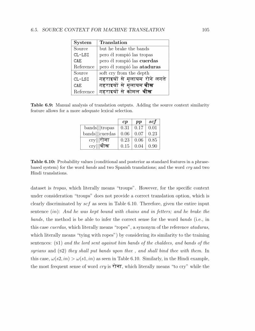
6.5. SOURCE CONTEXT FOR MACHINE TRANSLATION 105
System TranslationSource but he brake the bandsCL-LSI pero el rompio las tropasCAE pero el rompio las cuerdasReference pero el rompio las atadurasSource soft cry from the depthCL-LSI ghrAiyo\ s� m� lAym ron� lgt�CAE ghrAiyo\ s� m� lAym cFKReference ghrAiyo\ s� koml cFK
Table 6.9: Manual analysis of translation outputs. Adding the source context similarityfeature allows for a more adequate lexical selection.
cp pp scfbands|||tropas 0.31 0.17 0.01bands|||cuerdas 0.06 0.07 0.23
cry|||ronA 0.23 0.06 0.85cry|||cFK 0.15 0.04 0.90
Table 6.10: Probability values (conditional and posterior as standard features in a phrase-based system) for the word bands and two Spanish translations; and the word cry and twoHindi translations.
dataset is tropas, which literally means “troups”. However, for the specific context
under consideration “troups” does not provide a correct translation option, which is
clearly discriminated by scf as seen in Table 6.10. Therefore, given the entire input
sentence (in): And he was kept bound with chains and in fetters; and he brake the
bands , the method is be able to infer the correct sense for the word bands (i.e., in
this case cuerdas, which literally means “ropes”, a synonym of the reference ataduras,
which literally means “tying with ropes”) by considering its similarity to the training
sentences: (s1) and the lord sent against him bands of the chaldees, and bands of the
syrians and (s2) they shall put bands upon thee , and shall bind thee with them. In
this case, ω(s2, in) > ω(s1, in) as seen in Table 6.10. Similarly, in the Hindi example,
the most frequent sense of word cry is ronA, which literally means “to cry” while the
106 CHAPTER 6. CROSS-LANGUAGE INFORMATION RETRIEVAL
example in Table 6.9 refers to the sense of cry as cFK, which means to scream. Our
method could identify the context and hence the scf(cry|||cFK) > scf(cry|||ronA).
6.5.4 Scalability
There are two components of this method: (i) incorporation of source-context fea-
tures during the tuning phase of MT and projection of training sentences in the
latent space; and (ii) similarity estimation of the input sentence with the training
sentences in the latent space. The former step is computationally expensive but it
being one-time and offline, it is not a big concern. On the other hand, the similarity
estimation is online. It can be efficiently implemented by using a multi-core CPU or
GPU as it is essentially a matrix multiplication.

6.5. SOURCE CONTEXT FOR MACHINE TRANSLATION 107

Chapter 7Bottleneck dimensionality for autoencoders
Lately, dimensionality reduction techniques based on deep learning have become
very popular, especially deep autoencoders (Hinton and Salakhutdinov, 2006). Deep
autoencoders can extract highly useful and compact features from the structural
information of the data. Deep autoencoders have proven to be very effective in
learning reduced space representations of the data for similarity estimation (Hinton
and Salakhutdinov, 2006; Salakhutdinov and Hinton, 2009a). Deep learning is in-
spired by biological studies, which state the brain has a deep architecture. Despite
their high suitability to the task, deep learning did not find much audience until
Hinton and Salakhutdinov (2006) proposed a pre-training method to initialise the
network parameters in a good region for finding optimal solutions.
Although deep learning techniques are in vogue, there still exist some important
open questions. In most of the studies involving the use of these techniques for dimen-
sionality reduction, the qualitative analysis of the obtained projections is seldomly
presented. This makes the assessment of the reliability of learning very difficult.
109
110CHAPTER 7. BOTTLENECK DIMENSIONALITY FOR AUTOENCODERS
Typically, the reliability of the autoencoder is estimated based on its reconstruction
capability.
The first objective of this chapter is to introduce a novel framework for evaluat-
ing the quality of the low-dimensional embeddings produced by a deep autoencoder
based on the merits of the application under consideration. Concretely, the frame-
work is comprised of two metrics, structure preservation index (SPI) and similarity
accumulation index (SAI), which capture different aspects of the autoencoder’s re-
construction capabilities, including the structural distortion and similarities among
the reconstructed vectors (Gupta et al., 2016c). In this way, the framework gives
better insight of the autoencoder performance allowing for conducting better error
analysis and evaluation. The adequacy of the bottleneck dimension, referred to as
critical bottleneck dimensionality here, is rarely addressed in the literature. These
metrics also provide a better means for estimating the adequate size of critical bot-
tleneck dimensions.
The second objective is to conduct a comparative evaluation about the dimen-
sionality reduction capabilities of deep autoencoders across different languages. With
this empirical evaluation, we aim at shedding some light regarding the adequacy of
using the same number of dimensions when computing low-dimensional embeddings
for different languages, which is a common practice in the field.
The dimensionality reduction experiments presented in this chapter are carried
out on text at sentence level. The suitability of two types of deep autoencoders
(c.f. Section 3.4) is assessed: (i) deep autoencoder with stochastic RBM (bDA); and
(ii) deep autoencoder with multinomial RBM (rsDA). We report some interesting
findings at the architectural level with regards to the specific problem of modelling
text at the sentence level.
The chapter is structured as follows. Section 7.1 gives details about the analysis
framework of the autoencoder learning, experiments and results. The discussion on
critical bottleneck dimensionality and an automatic way to estimate it is given in
Section 7.2. In Section 7.3, we attempt to see whether any correlation exists between
7.1. QUALITATIVE ANALYSIS AND METRICS 111
the critical bottleneck dimensionality for a particular language and its perplexity.
7.1 Qualitative analysis and metrics
In this section, the metrics used for comparing the two considered autoencoder mod-
els (bDA and rsDA) are described. Subsequently, we present the comparative analysis
of the two models.
The quality of the projections and the sufficiency of a given dimensionality m
are measured by the autoencoder’s reconstruction ability. Unfortunately, the mean
squared error between the input x and its reconstruction x, referred to as recon-
struction error 3.12, is a poor measure of the quality of the obtained projections. It
neither gives any details about the quality of the reconstructions in terms of text data
representation nor the degree to which the structure of the data is preserved in the
reconstruction space. Moreover, it is difficult to justify the adequacy of bottleneck
dimensionality m by simply using the reconstruction error.
In the literature, when autoencoders are used for dimensionality reduction of text
data, the quality is measured in terms of the accuracy of the end-task, which may be
text categorisation (Hinton and Salakhutdinov, 2006), information retrieval (Salakhutdinov
and Hinton, 2009a), topic modeling (Salakhutdinov and Hinton, 2009b), term mod-
eling across scripts (Gupta et al., 2014) or sentiment prediction (Socher et al., 2011).
A shortcoming of this approach is that there is no way to estimate the full potential,
or upper bound, of the algorithm performance. On the other hand, in the case of
poor results, it becomes difficult to determine whether the training was proper or
not.
7.1.1 Metrics
In this chapter we introduce two new metrics, which are intended to capture differ-
ent aspects of the autoencoder’s reconstruction capability: (i) structure preservation
index (SPI), and (ii) similarity accumulation index (SAI). These two metrics focus
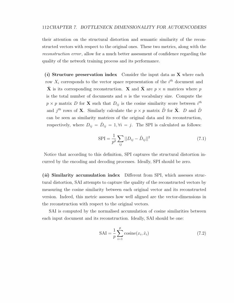
112CHAPTER 7. BOTTLENECK DIMENSIONALITY FOR AUTOENCODERS
their attention on the structural distortion and semantic similarity of the recon-
structed vectors with respect to the original ones. These two metrics, along with the
reconstruction error , allow for a much better assessment of confidence regarding the
quality of the network training process and its performance.
(i) Structure preservation index Consider the input data as X where each
row Xi corresponds to the vector space representation of the ith document and
X is its corresponding reconstruction. X and X are p × n matrices where p
is the total number of documents and n is the vocabulary size. Compute the
p × p matrix D for X such that Dij is the cosine similarity score between ith
and jth rows of X. Similarly calculate the p × p matrix D for X. D and D
can be seen as similarity matrices of the original data and its reconstruction,
respectively, where Dij = Dij = 1,∀i = j. The SPI is calculated as follows:
SPI =1
p2
∑ij
||Dij − Dij||2 (7.1)
Notice that according to this definition, SPI captures the structural distortion in-
curred by the encoding and decoding processes. Ideally, SPI should be zero.
(ii) Similarity accumulation index Different from SPI, which assesses struc-
tural distortion, SAI attempts to capture the quality of the reconstructed vectors by
measuring the cosine similarity between each original vector and its reconstructed
version. Indeed, this metric assesses how well aligned are the vector-dimensions in
the reconstruction with respect to the original vectors.
SAI is computed by the normalised accumulation of cosine similarities between
each input document and its reconstruction. Ideally, SAI should be one:
SAI =1
p
p∑i=1
cosine(xi, xi) (7.2)
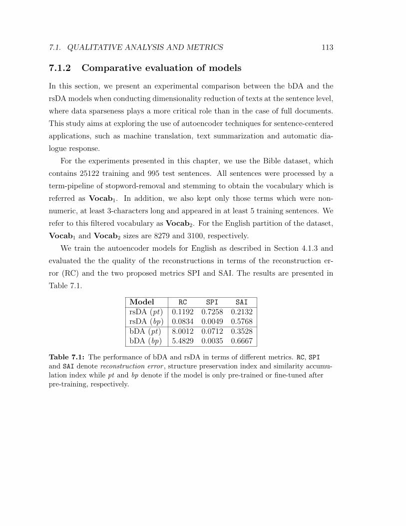
7.1. QUALITATIVE ANALYSIS AND METRICS 113
7.1.2 Comparative evaluation of models
In this section, we present an experimental comparison between the bDA and the
rsDA models when conducting dimensionality reduction of texts at the sentence level,
where data sparseness plays a more critical role than in the case of full documents.
This study aims at exploring the use of autoencoder techniques for sentence-centered
applications, such as machine translation, text summarization and automatic dia-
logue response.
For the experiments presented in this chapter, we use the Bible dataset, which
contains 25122 training and 995 test sentences. All sentences were processed by a
term-pipeline of stopword-removal and stemming to obtain the vocabulary which is
referred as Vocab1. In addition, we also kept only those terms which were non-
numeric, at least 3-characters long and appeared in at least 5 training sentences. We
refer to this filtered vocabulary as Vocab2. For the English partition of the dataset,
Vocab1 and Vocab2 sizes are 8279 and 3100, respectively.
We train the autoencoder models for English as described in Section 4.1.3 and
evaluated the the quality of the reconstructions in terms of the reconstruction er-
ror (RC) and the two proposed metrics SPI and SAI. The results are presented in
Table 7.1.
Model RC SPI SAI
rsDA (pt) 0.1192 0.7258 0.2132rsDA (bp) 0.0834 0.0049 0.5768bDA (pt) 8.0012 0.0712 0.3528bDA (bp) 5.4829 0.0035 0.6667
Table 7.1: The performance of bDA and rsDA in terms of different metrics. RC, SPIand SAI denote reconstruction error , structure preservation index and similarity accumu-lation index while pt and bp denote if the model is only pre-trained or fine-tuned afterpre-training, respectively.
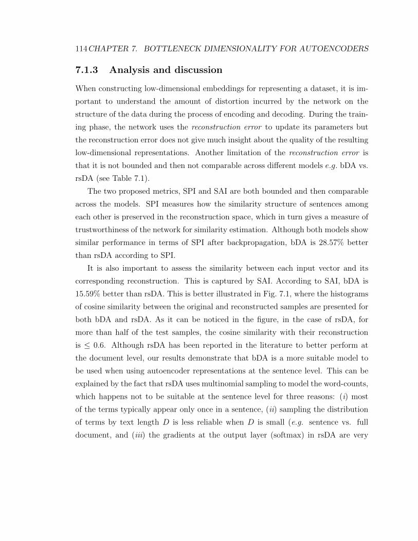
114CHAPTER 7. BOTTLENECK DIMENSIONALITY FOR AUTOENCODERS
7.1.3 Analysis and discussion
When constructing low-dimensional embeddings for representing a dataset, it is im-
portant to understand the amount of distortion incurred by the network on the
structure of the data during the process of encoding and decoding. During the train-
ing phase, the network uses the reconstruction error to update its parameters but
the reconstruction error does not give much insight about the quality of the resulting
low-dimensional representations. Another limitation of the reconstruction error is
that it is not bounded and then not comparable across different models e.g. bDA vs.
rsDA (see Table 7.1).
The two proposed metrics, SPI and SAI are both bounded and then comparable
across the models. SPI measures how the similarity structure of sentences among
each other is preserved in the reconstruction space, which in turn gives a measure of
trustworthiness of the network for similarity estimation. Although both models show
similar performance in terms of SPI after backpropagation, bDA is 28.57% better
than rsDA according to SPI.
It is also important to assess the similarity between each input vector and its
corresponding reconstruction. This is captured by SAI. According to SAI, bDA is
15.59% better than rsDA. This is better illustrated in Fig. 7.1, where the histograms
of cosine similarity between the original and reconstructed samples are presented for
both bDA and rsDA. As it can be noticed in the figure, in the case of rsDA, for
more than half of the test samples, the cosine similarity with their reconstruction
is ≤ 0.6. Although rsDA has been reported in the literature to better perform at
the document level, our results demonstrate that bDA is a more suitable model to
be used when using autoencoder representations at the sentence level. This can be
explained by the fact that rsDA uses multinomial sampling to model the word-counts,
which happens not to be suitable at the sentence level for three reasons: (i) most
of the terms typically appear only once in a sentence, (ii) sampling the distribution
of terms by text length D is less reliable when D is small (e.g. sentence vs. full
document, and (iii) the gradients at the output layer (softmax) in rsDA are very
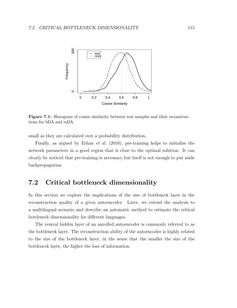
7.2. CRITICAL BOTTLENECK DIMENSIONALITY 115
0 0.2 0.4 0.6 0.8 1
030
0
Cosine Similarity
Fre
quen
cy
bDArsDA
Figure 7.1: Histogram of cosine similarity between test samples and their reconstruc-tions for bDA and rsDA.
small as they are calculated over a probability distribution.
Finally, as argued by Erhan et al. (2010), pre-training helps to initialise the
network parameters in a good region that is close to the optimal solution. It can
clearly be noticed that pre-training is necessary but itself is not enough to put aside
backpropagation.
7.2 Critical bottleneck dimensionality
In this section we explore the implications of the size of bottleneck layer in the
reconstruction quality of a given autoencoder. Later, we extend the analysis to
a multilingual scenario and describe an automatic method to estimate the critical
bottleneck dimensionality for different languages.
The central hidden layer of an unrolled autoencoder is commonly referred to as
the bottleneck layer. The reconstruction ability of the autoencoder is highly related
to the size of the bottleneck layer, in the sense that the smaller the size of the
bottleneck layer, the higher the loss of information.
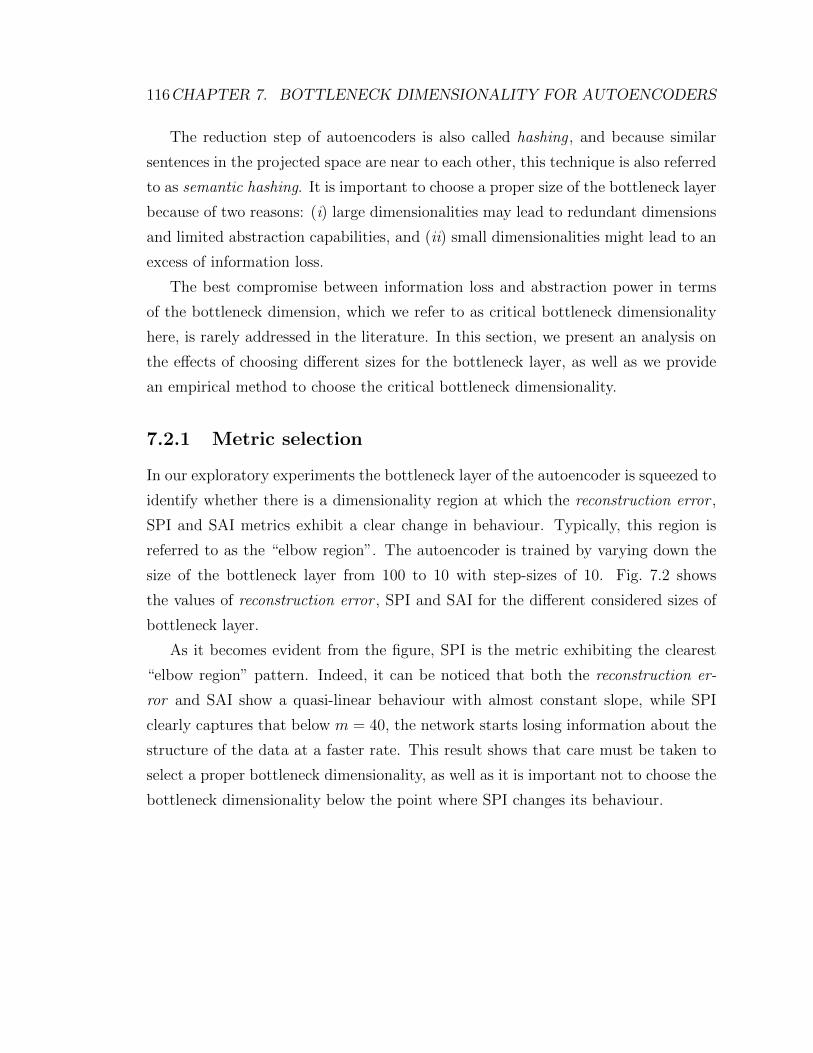
116CHAPTER 7. BOTTLENECK DIMENSIONALITY FOR AUTOENCODERS
The reduction step of autoencoders is also called hashing , and because similar
sentences in the projected space are near to each other, this technique is also referred
to as semantic hashing. It is important to choose a proper size of the bottleneck layer
because of two reasons: (i) large dimensionalities may lead to redundant dimensions
and limited abstraction capabilities, and (ii) small dimensionalities might lead to an
excess of information loss.
The best compromise between information loss and abstraction power in terms
of the bottleneck dimension, which we refer to as critical bottleneck dimensionality
here, is rarely addressed in the literature. In this section, we present an analysis on
the effects of choosing different sizes for the bottleneck layer, as well as we provide
an empirical method to choose the critical bottleneck dimensionality.
7.2.1 Metric selection
In our exploratory experiments the bottleneck layer of the autoencoder is squeezed to
identify whether there is a dimensionality region at which the reconstruction error ,
SPI and SAI metrics exhibit a clear change in behaviour. Typically, this region is
referred to as the “elbow region”. The autoencoder is trained by varying down the
size of the bottleneck layer from 100 to 10 with step-sizes of 10. Fig. 7.2 shows
the values of reconstruction error , SPI and SAI for the different considered sizes of
bottleneck layer.
As it becomes evident from the figure, SPI is the metric exhibiting the clearest
“elbow region” pattern. Indeed, it can be noticed that both the reconstruction er-
ror and SAI show a quasi-linear behaviour with almost constant slope, while SPI
clearly captures that below m = 40, the network starts losing information about the
structure of the data at a faster rate. This result shows that care must be taken to
select a proper bottleneck dimensionality, as well as it is important not to choose the
bottleneck dimensionality below the point where SPI changes its behaviour.
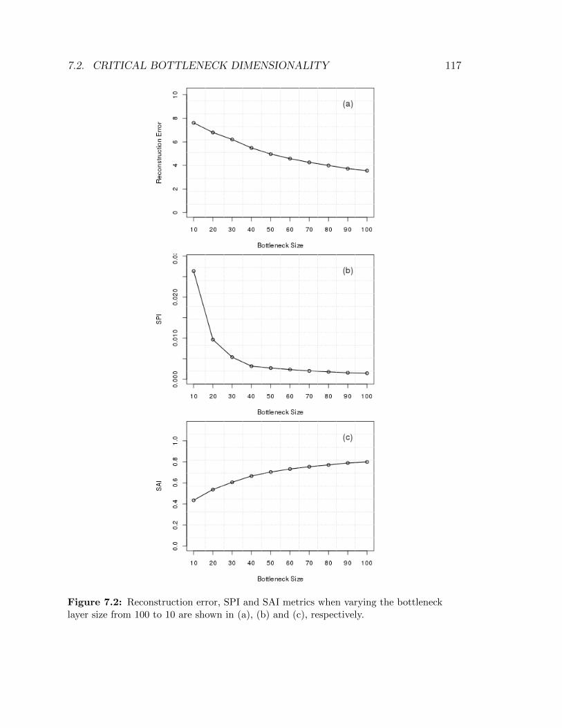
7.2. CRITICAL BOTTLENECK DIMENSIONALITY 117
Figure 7.2: Reconstruction error, SPI and SAI metrics when varying the bottlenecklayer size from 100 to 10 are shown in (a), (b) and (c), respectively.
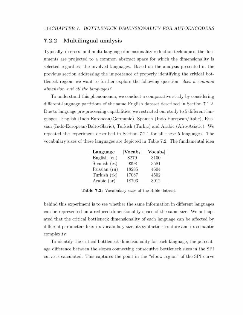
118CHAPTER 7. BOTTLENECK DIMENSIONALITY FOR AUTOENCODERS
7.2.2 Multilingual analysis
Typically, in cross- and multi-language dimensionality reduction techniques, the doc-
uments are projected to a common abstract space for which the dimensionality is
selected regardless the involved languages. Based on the analysis presented in the
previous section addressing the importance of properly identifying the critical bot-
tleneck region, we want to further explore the following question: does a common
dimension suit all the languages?
To understand this phenomenon, we conduct a comparative study by considering
different-language partitions of the same English dataset described in Section 7.1.2.
Due to language pre-processing capabilities, we restricted our study to 5 different lan-
guages: English (Indo-European/Germanic), Spanish (Indo-European/Italic), Rus-
sian (Indo-European/Balto-Slavic), Turkish (Turkic) and Arabic (Afro-Asiatic). We
repeated the experiment described in Section 7.2.1 for all these 5 languages. The
vocabulary sizes of these languages are depicted in Table 7.2. The fundamental idea
Language |Vocab1| |Vocab2|English (en) 8279 3100Spanish (es) 9398 3581Russian (ru) 18285 4504Turkish (tk) 17087 4502Arabic (ar) 18703 3012
Table 7.2: Vocabulary sizes of the Bible dataset.
behind this experiment is to see whether the same information in different languages
can be represented on a reduced dimensionality space of the same size. We anticip-
ated that the critical bottleneck dimensionality of each language can be affected by
different parameters like: its vocabulary size, its syntactic structure and its semantic
complexity.
To identify the critical bottleneck dimensionality for each language, the percent-
age difference between the slopes connecting consecutive bottleneck sizes in the SPI
curve is calculated. This captures the point in the “elbow region” of the SPI curve
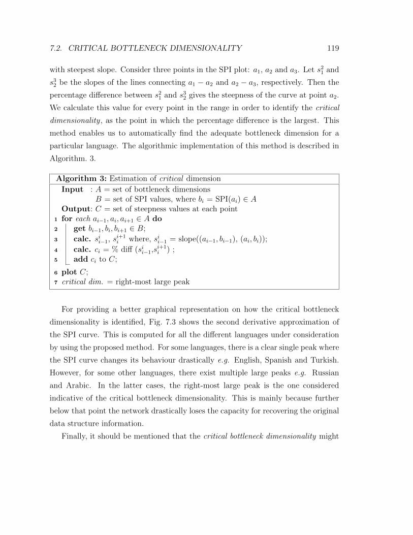
7.2. CRITICAL BOTTLENECK DIMENSIONALITY 119
with steepest slope. Consider three points in the SPI plot: a1, a2 and a3. Let s21 and
s32 be the slopes of the lines connecting a1 − a2 and a2 − a3, respectively. Then the
percentage difference between s21 and s3
2 gives the steepness of the curve at point a2.
We calculate this value for every point in the range in order to identify the critical
dimensionality , as the point in which the percentage difference is the largest. This
method enables us to automatically find the adequate bottleneck dimension for a
particular language. The algorithmic implementation of this method is described in
Algorithm. 3.
Algorithm 3: Estimation of critical dimension
Input : A = set of bottleneck dimensionsB = set of SPI values, where bi = SPI(ai) ∈ A
Output: C = set of steepness values at each point1 for each ai−1, ai, ai+1 ∈ A do2 get bi−1, bi, bi+1 ∈ B;
3 calc. sii−1, si+1i where, sii−1 = slope((ai−1, bi−1), (ai, bi));
4 calc. ci = % diff (sii−1,si+1i ) ;
5 add ci to C;
6 plot C;7 critical dim. = right-most large peak
For providing a better graphical representation on how the critical bottleneck
dimensionality is identified, Fig. 7.3 shows the second derivative approximation of
the SPI curve. This is computed for all the different languages under consideration
by using the proposed method. For some languages, there is a clear single peak where
the SPI curve changes its behaviour drastically e.g. English, Spanish and Turkish.
However, for some other languages, there exist multiple large peaks e.g. Russian
and Arabic. In the latter cases, the right-most large peak is the one considered
indicative of the critical bottleneck dimensionality. This is mainly because further
below that point the network drastically loses the capacity for recovering the original
data structure information.
Finally, it should be mentioned that the critical bottleneck dimensionality might
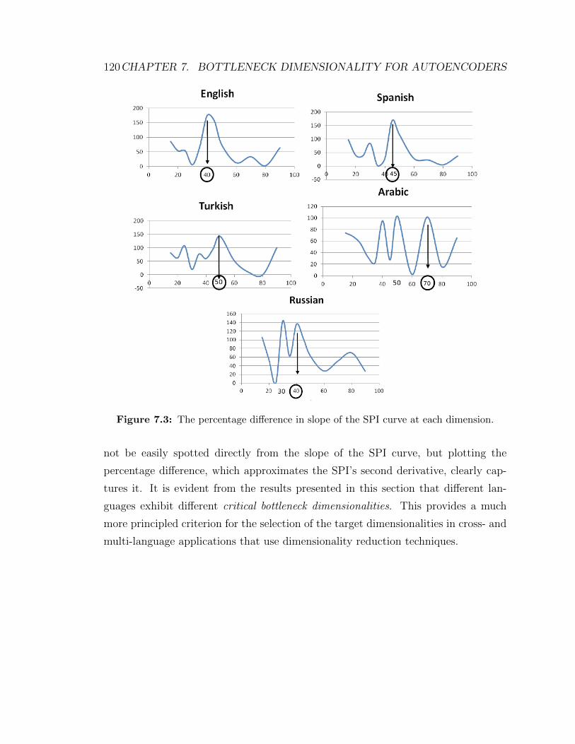
120CHAPTER 7. BOTTLENECK DIMENSIONALITY FOR AUTOENCODERS
Figure 7.3: The percentage difference in slope of the SPI curve at each dimension.
not be easily spotted directly from the slope of the SPI curve, but plotting the
percentage difference, which approximates the SPI’s second derivative, clearly cap-
tures it. It is evident from the results presented in this section that different lan-
guages exhibit different critical bottleneck dimensionalities. This provides a much
more principled criterion for the selection of the target dimensionalities in cross- and
multi-language applications that use dimensionality reduction techniques.
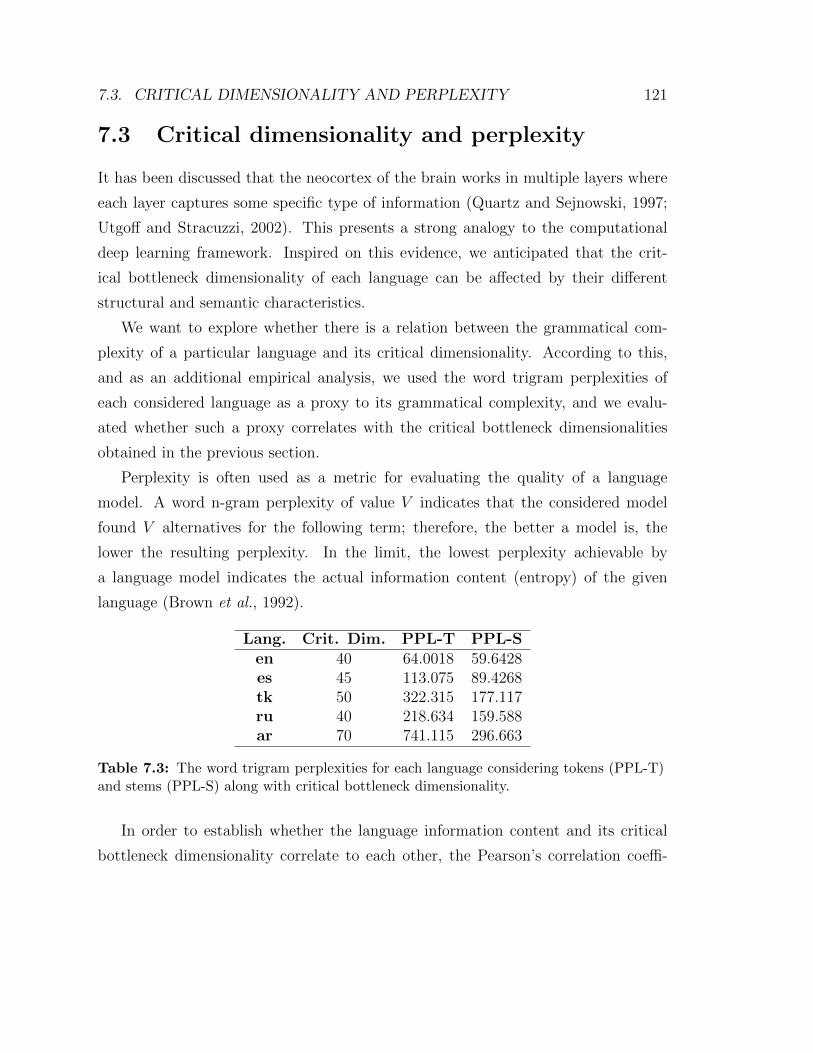
7.3. CRITICAL DIMENSIONALITY AND PERPLEXITY 121
7.3 Critical dimensionality and perplexity
It has been discussed that the neocortex of the brain works in multiple layers where
each layer captures some specific type of information (Quartz and Sejnowski, 1997;
Utgoff and Stracuzzi, 2002). This presents a strong analogy to the computational
deep learning framework. Inspired on this evidence, we anticipated that the crit-
ical bottleneck dimensionality of each language can be affected by their different
structural and semantic characteristics.
We want to explore whether there is a relation between the grammatical com-
plexity of a particular language and its critical dimensionality. According to this,
and as an additional empirical analysis, we used the word trigram perplexities of
each considered language as a proxy to its grammatical complexity, and we evalu-
ated whether such a proxy correlates with the critical bottleneck dimensionalities
obtained in the previous section.
Perplexity is often used as a metric for evaluating the quality of a language
model. A word n-gram perplexity of value V indicates that the considered model
found V alternatives for the following term; therefore, the better a model is, the
lower the resulting perplexity. In the limit, the lowest perplexity achievable by
a language model indicates the actual information content (entropy) of the given
language (Brown et al., 1992).
Lang. Crit. Dim. PPL-T PPL-Sen 40 64.0018 59.6428es 45 113.075 89.4268tk 50 322.315 177.117ru 40 218.634 159.588ar 70 741.115 296.663
Table 7.3: The word trigram perplexities for each language considering tokens (PPL-T)and stems (PPL-S) along with critical bottleneck dimensionality.
In order to establish whether the language information content and its critical
bottleneck dimensionality correlate to each other, the Pearson’s correlation coeffi-
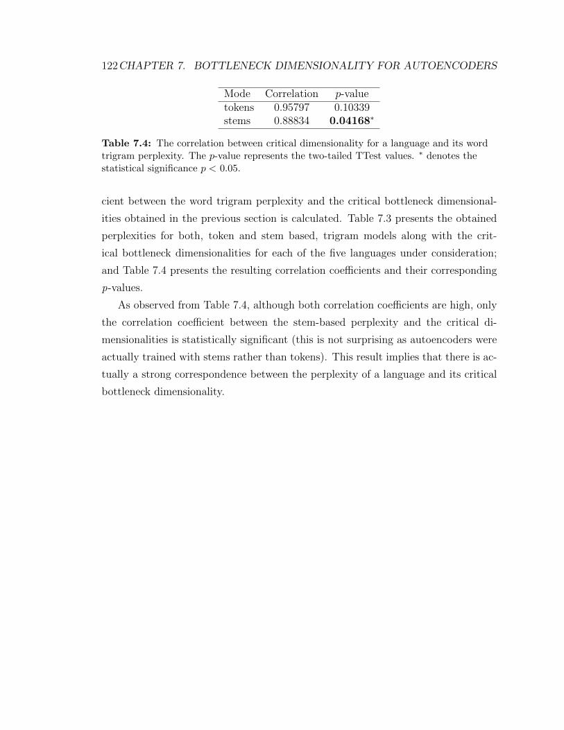
122CHAPTER 7. BOTTLENECK DIMENSIONALITY FOR AUTOENCODERS
Mode Correlation p-valuetokens 0.95797 0.10339stems 0.88834 0.04168∗
Table 7.4: The correlation between critical dimensionality for a language and its wordtrigram perplexity. The p-value represents the two-tailed TTest values. ∗ denotes thestatistical significance p < 0.05.
cient between the word trigram perplexity and the critical bottleneck dimensional-
ities obtained in the previous section is calculated. Table 7.3 presents the obtained
perplexities for both, token and stem based, trigram models along with the crit-
ical bottleneck dimensionalities for each of the five languages under consideration;
and Table 7.4 presents the resulting correlation coefficients and their corresponding
p-values.
As observed from Table 7.4, although both correlation coefficients are high, only
the correlation coefficient between the stem-based perplexity and the critical di-
mensionalities is statistically significant (this is not surprising as autoencoders were
actually trained with stems rather than tokens). This result implies that there is ac-
tually a strong correspondence between the perplexity of a language and its critical
bottleneck dimensionality.

7.3. CRITICAL DIMENSIONALITY AND PERPLEXITY 123

Chapter 8Conclusions & future work
In this Chapter we present the concluding remarks of the main finding of this
dissertation (Section 8.1), discuss limitations (Section 8.2) and outline the potential
future work (Section 8.4).
8.1 Conclusions
This dissertation deals with cross-view projection techniques for cross-view inform-
ation retrieval tasks. In the exploration, a very important and prevalent problem
of mixed-script IR is formally defined and investigated. The deep learning based
neural cross-view models proposed in this dissertation provide state-of-the-art per-
formance for various cross-language and cross-script applications. The dissertation
also explored the architectural properties of the autoencoders which has attained less
attention and establishes the notion of critical bottleneck dimensionality.
In this dissertation, the problem of mixed-script IR is introduced formally and
motivated as a cross-view problem and the involved research challenges are presented.
125
126 CHAPTER 8. CONCLUSIONS
We also conducted a quantitative analysis on how much web search traffic is actually
affected by MSIR through a large-scale empirical study of a commercial search engine
query logs. This analysis has provided a lot of insight on the prevalence and impact
of the MSIR behaviour on the web (RQ1). A principled solution to address the
primary challenge of MSIR, the term variations across the scripts, is proposed in
form of a cross-view autoencoder. The proposed mixed-script joint model learns
abstract representation of terms across the scripts through deep learning architecture
such that term equivalents are close to each other. The deep autoencoder based
approach provides highly discriminative and powerful representation for terms with
as low as 20 dimensions. An extensive empirical analysis is presented on a practical
and important use-case: ad-hoc retrieval of songs lyrics. The experiments suggest
that the state-of-the-art methods for handling spelling variation and transliteration
mining have strong effect on the performance of IR in mixed-script space but the
cross-view autoencoder significantly outperforms them (RQ1).
Cross-view autoencoders provide the best way to model terms across scripts be-
cause of the small and finite feature space as discussed in Section 4.1.2. They do
not perform as strongly for modelling of cross-language documents which involve
unbounded and large feature space. The external data composition neural network
(XCNN) model, proposed in this dissertation, overcomes such limitations of the
cross-view autoencoder for modelling cross-language text. We have presented and
evaluated the XCNN framework on different cross-language tasks and found it to
be statistically superior in performance to other strong baselines (RQ2). These two
attributes of the XCNN model prove crucial for its performance in the retrieval tasks:
(i) the learning framework proposed in this work gives a natural way to extend ex-
ternal relevance signals available in the form of pseudo relevance or clickthrough data
to cross-language embeddings with the help of a small subset of parallel data, and
(ii) the non-linear composition model optimises an objective function that directly
relates to the considered task evaluation metric. These properties allow for the model
to perform better than other latent semantic models which rely only on parallel data
8.1. CONCLUSIONS 127
for training.
The gradient based learning provides a way to scale up to large training data-
sets more easily than linear methods that depend on matrix factorization, such as
CL-LSI and OPCA. For XCNN, the time and space complexity grow linearly with
the size of the vocabulary and the amount of training datapoints, while complexity
grows quadratically for models based on matrix factorization. The XCNN model also
outperforms the S2Net model, the only latent semantic model that optimises a loss
function directly related to the evaluation metric. The use of non-linearity allows the
model to learn interesting dependence between the terms across languages compared
to their linear counterparts.
We have also explored a novel methodology to effectively include a deep learn-
ing based contextual similarity estimation, which handles source context for ma-
chine translation (RQ3). This feature is successfully incorporated in an end-to-end
SMT system. The method shows statistically significant improvements compared to
strong baseline systems in English-to-Spanish and English-to-Hindi translation tasks.
Manual analysis confirmed the advantages of choosing the appropriate translation
unit by taking into account the information of the input sentence context and the
relation with the training sentences evidenced by the deep source context feature.
Finally, we have presented a comprehensive study on the use of autoencoders for
modelling text data at the sentence level. Particularly, we explored the suitability
of two different models, binary deep autoencoder (bDA) and replicated softmax
deep autoencoder (rsDA), for constructing deep autoencoder representations of text
data. In order to evaluate the quality of autoencoder generated representations,
we defined and evaluated two novel metrics related to the reconstruction property
of an autoencoder: structure preservation index (SPI) and similarity accumulation
index (SAI). We also introduced the concept of critical bottleneck dimensionality
(CBD) below which the structural information is lost for text representation with
autoencoders. We have also proposed an automatic method to find the CBD using the
SPI metric, which allows for a better discrimination and identification of CBD (RQ4).
128 CHAPTER 8. CONCLUSIONS
Our analysis of CBD across different languages has suggested there is a correlation
between the critical bottleneck dimensionality and language perplexity.
8.2 Limitations
In this section we list the limitations of the methods presented in this dissertation.
Parallel/comparable data: Most of the models discussed in this dissertation
assume that parallel or comparable data are available. In reality, such resources are
very limited and almost non-existent for many languages. Small amounts of parallel
data lead to poor performance for bilingual models especially in case of resource-poor
languages. Although we have tried to address this issue in the XCNN model where
it is initialised using monolingual data and then fine-tuned using small amount of
cross-lingual data, such models are not applicable to language pairs for which no
parallel data are available.
External relevance signals: In the XCNN model, we need external relevance sig-
nals such as relevance judgements or clickthrough data. The former is more expens-
ive to obtain than the latter. Although we have tried to generate pseudo-relevance
signals using standard retrieval models, they are not as effective as actual signals.
Computational resources: Training large neural networks on large datasets re-
quire heavy computational resources. Modelling all the terms present in the corpus is
also a big challenge through neural networks because of enormously large and sparse
visible layers. In order to perform such experiments, we used GPU’s and assumed
their availability. Although there are approaches like word-hashing where the terms
are coded by their character n-grams to reduce the feature space, their suitability
for cross-language models is still to be investigated.
8.3. CODE 129
Mixed-script data: Being a relatively new area, there is negligible amount of
public data available for mixed-script IR. We have developed the first such datasets
for Hindi and made available through FIRE shared task on mixed-script IR (Saha Roy
et al., 2013; Choudhury et al., 2014). Similarly, the training data for modelling
mixed-script terms is also very scarce. Although traditional transliteration data are
available, they do not represent the spelling variations within the script well. The
CAE model assumes the availability of such data.
Evaluation metrics for mixed-script terms: Currently MSIR is being evalu-
ated by the quality of retrieval in ad-hoc retrieval setting. We believe there is a need
to device evaluation metrics which capture how close is the transliterated query term
to the actual term in order to allow qualitative analysis.
8.3 Code
In order to promote replicability, we have made the code publicly available as much
as possible. The code also contains details on parameter tuning details. The code
related to cross-view autoencoder for mixed-script IR is available at: http://users.
dsic.upv.es/~pgupta/mixed-script-ir.html, the code for XCNN is available at:
https://github.com/parthg/jDNN
8.4 Future work
8.4.1 Mixed-script IR
In this dissertation, we have conducted some initial research in the emerging area of
mixed-script IR. Future work in this area must also deal with the related problem
of code-mixing in queries and documents. Code-mixing is a growing phenomenon in
the user-generated content and provide additional challenges for MSIR. Similarly, one
130 CHAPTER 8. CONCLUSIONS
should also extend the MSIR framework to a more general setup such as mixed-script
multilingual IR.
8.4.2 Composition neural networks
The external relevance composition neural network (XCNN) model provides a state-
of-the-art performance for many CLIR applications. This model provides a natural
way of incorporating semantic compositional models. One can extend this model
with such techniques to obtain richer representation of text data depending on the
requirement of the application. We believe such techniques may provide very effect-
ive performance for more sophisticated tasks such as semantic textual entailment
compared to information retrieval.
8.4.3 Source context features
Interesting future work on source context features using deep autoencoder as presen-
ted in this work should focus on better integrating the dynamic feature into trans-
lation decoding at the architecture level. In its current form, it lies as an additional
layer to the existing phrase-based machine translation system. This also increases
the search time. To speed-up search, one can divide the feature space in chunks and
search hierarchically, perform clustering or use kd-trees like data structures.
8.4.4 Qualitative metrics
One possible extension of our study on suitability of the proposed metrics, especially
SPI, should focus on using the proposed metrics as error metrics during the autoen-
coder fine tuning stage. If this metric can be used along with back-propagation, we
envisage a new generation of text-oriented autoencoders that will be able to provide
a much better characterization of the linguistic phenomenon in text data. Another
future extension will be to validate the impact of the proposed metrics using extrinsic
evaluation.
8.4. FUTURE WORK 131
8.4.5 More applications
We also want to extend the models from this thesis to more cross-view applications
such as: (i) enriching bilingual dictionaries (Dubey et al., 2014); (ii) discovering
parallel and reused text in news stories (Gupta et al., 2013b); and (iii) cross-language
text categorisation (Klementiev et al., 2012).

Bibliography
Adafre, S. F. and de Rijke, M. (2006). Finding similar sentences across multiple
languages in wikipedia. In Proceedings of the EACL Workshop on New Text:
Wikis and Blogs and Other Dynamic Text Sources , EACL ’06, pages 62–69.
Ahmed, U. Z., Bali, K., Choudhury, M., and VB, S. (2011). Challenges in designing
input method editors for indian lan-guages: The role of word-origin and context.
In Proceedings of the Workshop on Advances in Text Input Methods , WTIM ’11,
pages 1–9.
Amati, G. (2006). Frequentist and bayesian approach to information retrieval. In Pro-
ceedings of the 28th European Conference on Advances in Information Retrieval ,
ECIR’06, pages 13–24, Berlin, Heidelberg. Springer-Verlag.
Anderka, M. and Stein, B. (2009). The esa retrieval model revisited. In Proceedings
of the 32Nd International ACM SIGIR Conference on Research and Development
in Information Retrieval , SIGIR ’09, pages 670–671, New York, NY, USA. ACM.
Banchs, R. E. and Costa-jussa, M. R. (2011). A semantic feature for statistical
machine translation. In Proceedings of the Fifth Workshop on Syntax, Semantics
and Structure in Statistical Translation, SSST-5, pages 126–134.
Banchs, R. E. and Kaltenbrunner, A. (2008). Exploiting mds projections for cross-
133
134 BIBLIOGRAPHY
language ir. In Proceedings of the 31st Annual International ACM SIGIR Con-
ference on Research and Development in Information Retrieval , SIGIR ’08, pages
863–864, New York, NY, USA. ACM.
Banerjee, S. and Pedersen, T. (2003). Extended gloss overlaps as a measure of
semantic relatedness. In Proceedings of the 18th International Joint Conference on
Artificial Intelligence, IJCAI’03, pages 805–810, San Francisco, CA, USA. Morgan
Kaufmann Publishers Inc.
Bar-Yossef, Z. and Kraus, N. (2011). Context-sensitive query auto-completion. In
Proceedings of the 20th International Conference on World Wide Web, WWW ’11,
pages 107–116, New York, NY, USA. ACM.
Barron-Cedeno, A., Rosso, P., Agirre, E., and Labaka, G. (2010). Plagiarism detec-
tion across distant language pairs. In Proceedings of the 23rd International Con-
ference on Computational Linguistics , COLING ’10, pages 37–45, Stroudsburg,
PA, USA. Association for Computational Linguistics.
Barron-Cedeno, A. (2012). On the mono- and cross-language detection of text re-use
and plagiarism. Ph.D. thesis, Universitat Politenica de Valencia.
Barron-Cedeno, A., Rosso, P., Pinto, D., and Juan, A. (2008). On cross-lingual
plagiarism analysis using a statistical model. In Proceedings of the Workshop on
Uncovering Plagiarism, Authorship and Social Software Misuse, ECAI’08.
Barron-Cedeno, A., Gupta, P., and Rosso, P. (2013). Methods for cross-language
plagiarism detection. Knowledge-Based Systems , 50, 211–217.
Bast, H. and Weber, I. (2006). Type less, find more: Fast autocompletion search
with a succinct index. In Proceedings of the 29th Annual International ACM
SIGIR Conference on Research and Development in Information Retrieval , SIGIR
’06, pages 364–371, New York, NY, USA. ACM.
BIBLIOGRAPHY 135
Blei, D. M., Ng, A. Y., and Jordan, M. I. (2003). Latent dirichlet allocation. Journal
of Machine Learning Research, 3, 993–1022.
Bojar, O., Buck, C., Federmann, C., Haddow, B., Koehn, P., Leveling, J., Monz,
C., Pecina, P., Post, M., Saint-Amand, H., Soricut, R., Specia, L., and Tamchyna,
A. (2014a). Findings of the 2014 workshop on statistical machine translation.
In Proceedings of the Ninth Workshop on Statistical Machine Translation, pages
12–58, Baltimore, Maryland, USA. Association for Computational Linguistics.
Bojar, O., Diatka, V., Rychly, P., Stranak, P., Suchomel, V., Tamchyna, A., and
Zeman, D. (2014b). Hindencorp - hindi-english and hindi-only corpus for machine
translation. In Proceedings of the Ninth International Conference on Language
Resources and Evaluation, LREC’14, Reykjavik, Iceland.
Bourlard, H. and Kamp, Y. (1988). Auto-association by multilayer perceptrons and
singular value decomposition. Biological Cybernetics , 59(4), 291–294.
Braschler, M. (2004). Combination approaches for multilingual text retrieval. In-
formation Retrieval , 7(1-2), 183–204.
Braschler, M., Krause, J., Peters, C., and Schauble, P. (1998). Cross-language in-
formation retrieval (CLIR) track overview. In Proceedings of The Seventh Text
REtrieval Conference, TREC 1998, Gaithersburg, Maryland, USA, November 9-
11, 1998 , pages 1–8.
Braschler, M., Schauble, P., and Peters, C. (1999). Cross-language information re-
trieval (CLIR) track overview. In Proceedings of The Eighth Text REtrieval Con-
ference, TREC 1999, Gaithersburg, Maryland, USA, November 17-19, 1999 .
Bromley, J., Guyon, I., LeCun, Y., Sackinger, E., and Shah, R. (1993). Signature
verification using a siamese time delay neural network. In Proceedings of Advances
in Neural Information Processing Systems Conference, Denver, Colorado, USA,
NIPS’ 93, pages 737–744.
136 BIBLIOGRAPHY
Brown, P. F., Pietra, V. J. D., Mercer, R. L., Pietra, S. A. D., and Lai, J. C. (1992).
An estimate of an upper bound for the entropy of english. Comput. Linguist.,
18(1), 31–40.
Burges, C. (2010). Dimension reduction: A guided tour. Foundations and Trends in
Machine Learning .
Carterette, B., Kanoulas, E., Hall, M. M., and Clough, P. D. (2014). Overview of
the TREC 2014 session track. In Proceedings of The Twenty-Third Text REtrieval
Conference, TREC 2014, Gaithersburg, Maryland, USA, November 19-21, 2014 .
Ceska, Z., Toman, M., and Jezek, K. (2008). Multilingual Plagiarism Detection. In
Proceedings of the 13th International Conference on Artificial Intelligence (ICAI
2008), pages 83–92, Varna, Bulgaria. Springer-Verlag.
Chandar A. P., S., Lauly, S., Larochelle, H., Khapra, M. M., Ravindran, B., Raykar,
V. C., and Saha, A. (2014). An autoencoder approach to learning bilingual word
representations. In Advances in Neural Information Processing Systems 27: An-
nual Conference on Neural Information Processing Systems 2014, December 8-13
2014, Montreal, Quebec, Canada, pages 1853–1861.
Chen, H.-H., Hueng, S.-J., Ding, Y.-W., and Tsai, S.-C. (1998). Proper name trans-
lation in cross-language information retrieval. In Proceedings of the 36th Annual
Meeting of the Association for Computational Linguistics and 17th International
Conference on Computational Linguistics - Volume 1 , ACL ’98, pages 232–236,
Stroudsburg, PA, USA. Association for Computational Linguistics.
Choudhury, M., Bali, K., Gupta, K., and Datha, N. (2012). Multilingual search for
transliterated content. Patent number US 20120278302.
Choudhury, M., Chittaranjan, G., Gupta, P., and Das, A. (2014). Overview of FIRE
2014 track on transliterated search. In Sixth Forum for Information Retrieval
Evaluation, FIRE ’14.
BIBLIOGRAPHY 137
Church, K. (1993). Char align: A Program for Aligning Parallel Texts at the Char-
acter Level. In Proceedings of the 31st Annual Meeting of the Association for Com-
putational Linguistics , ACL ’93, pages 1–8, Columbus, OH, USA. Association for
Computational Linguistics.
Costa-jussa, M. R., Gupta, P., Rosso, P., and Banchs, R. E. (2014). English-to-hindi
system description for WMT 2014: Deep source-context features for Moses. In
Proceedings of the Ninth Workshop on Statistical Machine Translation, WMT ’14,
pages 79–83, Baltimore, Maryland, USA. Association for Computational Linguist-
ics.
Cox, T. F. and Cox, M. (2000). Multidimensional Scaling . CRC Press, Boca Raton,
FL, USA.
Dash, M. and Liu, H. (1997). Feature selection for classification. Intelligent Data
Analysis , 1, 131–156.
Deerwester, S. C., Dumais, S. T., Landauer, T. K., Furnas, G. W., and Harshman,
R. A. (1990). Indexing by latent semantic analysis. JASIS , 41(6), 391–407.
Diamantaras, K. I. and Kung, S. Y. (1996). Principal Component Neural Networks:
Theory and Applications . John Wiley & Sons, Inc., New York, NY, USA.
Dua, N., Gupta, K., Choudhury, M., and Bali, K. (2011). Query completion without
query logs for song search. In Proceedings of WWW (Companion Volume), pages
31–32.
Dubey, A., Gupta, P., Varma, V., and Rosso, P. (2014). Enrichment of bilingual
dictionary through news stream data. In Proceedings of the Ninth International
Conference on Language Resources and Evaluation, LREC ’14, pages 3761–3765.
Dumais, S., Landauer, T. K., and Littman, M. L. (1997). Automatic Cross-Linguistic
Information Retrieval using Latent Semantic Indexing. In AAAI-97 Spring Sym-
posium Series: Cross-Language Text and Speech Retrieval , pages 18–24.
138 BIBLIOGRAPHY
Durrani, N., Haddow, B., Koehn, P., and Heafield, K. (2014). Edinburgh’s phrase-
based machine translation systems for WMT-14. In Proceedings of the Ninth Work-
shop on Statistical Machine Translation, WMT ’14, Baltimore, Maryland, USA.
Association for Computational Linguistics.
Efthimiadis, E. N. (2008). How do greeks search the web?: A query log analysis
study. In Proceedings of iNEWS , pages 81–84.
Efthimiadis, E. N., Malevris, N., Kousaridas, A., Lepeniotou, A., and Loutas, N.
(2009). Non-english web search: an evaluation of indexing and searching the greek
web. Information Retrieval , 12(3).
Erhan, D., Bengio, Y., Courville, A., Manzagol, P.-A., Vincent, P., and Bengio,
S. (2010). Why does unsupervised pre-training help deep learning? Journal of
Machine Learning Research, 11, 625–660.
Fellbaum, C. (1998). WordNet: An electronic lexical database. Bradford Books.
Fodor, I. (2002). A survey of dimension reduction techniques. Technical report,
LLNL technical report, UCRL ID-148494.
Franco-Salvador, M., Gupta, P., and Rosso, P. (2013). Cross-language plagiarism de-
tection using a multilingual semantic network. In Proceedings of the 35th European
Conference on Advances in Information Retrieval , ECIR’13, pages 710–713, Ber-
lin, Heidelberg. Springer-Verlag.
Franco-Salvador, M., Rosso, P., and Navigli, R. (2014). A knowledge-based repres-
entation for cross-language document retrieval and categorization. In Proceedings
of the 14th Conference of the European Chapter of the Association for Computa-
tional Linguistics , pages 414–423. Association for Computational Linguistics.
Franco-Salvador, M., Gupta, P., Rosso, P., and Banchs, R. E. (2016). Cross-language
plagiarism detection over continuous-space- and knowledge graph-based represent-
ations of language. Knowledge-Based Systems , 111, 87–98.
BIBLIOGRAPHY 139
Franco-Salvador, M., Rosso, P., and Montes-y-Gomez, M. (2016). A systematic study
of knowledge graph analysis for cross-language plagiarism detection. Information
Processing & Management , 52(4), 550–570.
French, J. C., Powell, A. L., and Schulman, E. (1997). Applications of approximate
word matching in information retrieval. In Proceedings of the Sixth International
Conference on Information and Knowledge Management , CIKM ’97, pages 9–15,
New York, NY, USA. ACM.
Fung, P. and Cheung, P. (2004). Multi-level bootstrapping for extracting parallel
sentences from a quasi-comparable corpus. In Proceedings of the 20th International
Conference on Computational Linguistics , COLING ’04, Stroudsburg, PA, USA.
Association for Computational Linguistics.
Gabrilovich, E. and Markovitch, S. (2007). Computing semantic relatedness using
wikipedia-based explicit semantic analysis. In Proceedings of the 20th interna-
tional joint conference on Artifical intelligence, IJCAI’07, pages 1606–1611, San
Francisco, CA, USA. Morgan Kaufmann Publishers Inc.
Gao, J., Nie, J.-Y., Xun, E., Zhang, J., Zhou, M., and Huang, C. (2001). Improving
query translation for cross-language information retrieval using statistical models.
In Proceedings of the 24th Annual International ACM SIGIR Conference on Re-
search and Development in Information Retrieval , SIGIR ’01, pages 96–104, New
York, NY, USA. ACM.
Gao, J., He, X., and Nie, J.-Y. (2010). Clickthrough-based translation models for
web search: From word models to phrase models. In Proceedings of the 19th ACM
International Conference on Information and Knowledge Management , CIKM ’10,
pages 1139–1148, New York, NY, USA. ACM.
Gao, J., Toutanova, K., and Yih, W.-t. (2011). Clickthrough-based latent semantic
models for web search. In Proceedings of the 34th International ACM SIGIR
140 BIBLIOGRAPHY
Conference on Research and Development in Information Retrieval , SIGIR ’11,
pages 675–684, New York, NY, USA. ACM.
Gehler, P. V., Holub, A. D., and Welling, M. (2006). The rate adapting poisson
model for information retrieval and object recognition. In Proceedings of the 23rd
International Conference on Machine Learning , ICML ’06, pages 337–344, New
York, NY, USA. ACM.
Geng, X., Liu, T.-Y., Qin, T., and Li, H. (2007). Feature selection for ranking. In
Proceedings of the 30th Annual International ACM SIGIR Conference on Research
and Development in Information Retrieval , SIGIR ’07, pages 407–414, New York,
NY, USA. ACM.
Gupta, K., Choudhury, M., and Bali, K. (2012a). Mining Hindi-English transliter-
ation pairs from online Hindi lyrics. In Proceedings of the Eighth International
Conference on Language Resources and Evaluation, LREC’12, pages 2459–2465.
Gupta, P. (2014). Modelling of terms across scripts through autoencoders. In Pro-
ceedings of the 37th International ACM SIGIR Conference on Research & Devel-
opment in Information Retrieval , SIGIR ’14, pages 1279–1279, New York, NY,
USA. ACM.
Gupta, P. and Rosso, P. (2012a). Expected divergence based feature selection for
learning to rank. In Proceedings of the 24th International Conference on Compu-
tational Linguistics , COLING ’12, pages 431–440.
Gupta, P. and Rosso, P. (2012b). Text reuse with ACL: (Upward) Trends. In Proceed-
ings of the ACL-2012 Special Workshop on Rediscovering 50 Years of Discoveries ,
ACL ’12, pages 76–82, Stroudsburg, PA, USA. Association for Computational
Linguistics.
Gupta, P., Barron-Cedeno, A., and Rosso, P. (2012b). Cross-language high similarity
search using a conceptual thesaurus. In Proceedings of the Third International
BIBLIOGRAPHY 141
Conference on Information Access Evaluation: Multilinguality, Multimodality, and
Visual Analytics , CLEF ’12, pages 67–75, Berlin, Heidelberg. Springer-Verlag.
Gupta, P., Rosso, P., and Banchs, R. E. (2013a). Encoding transliteration variation
through dimensionality reduction: FIRE Shared Task on Transliterated Search. In
Fifth Forum for Information Retrieval Evaluation, FIRE ’13.
Gupta, P., Clough, P. D., Rosso, P., Stevenson, M., and Banchs, R. E. (2013b).
PAN@FIRE: Overview of the Cross-Language !ndian News Story Search (CL!NSS)
track. In Fifth Forum for Information Retrieval Evaluation, FIRE ’13.
Gupta, P., Bali, K., Banchs, R. E., Choudhury, M., and Rosso, P. (2014). Query
expansion for mixed-script information retrieval. In Proceedings of the 37th In-
ternational ACM SIGIR Conference on Research & Development in Information
Retrieval , SIGIR ’14, pages 677–686, New York, NY, USA. ACM.
Gupta, P., Banchs, R. E., and Rosso, P. (2016a). Continuous space models for CLIR.
Information Processing & Management , 53(2), 359–370.
Gupta, P., Costa-Jussa, M. R., Rosso, P., and Banchs, R. E. (2016b). A deep source-
context feature for lexical selection in statistical machine translation. Pattern
Recognition Letters , 75, 24–29.
Gupta, P., Banchs, R. E., and Rosso, P. (2016c). Squeezing bottlenecks: Exploring
the limits of autoencoder semantic representation capabilities. Neurocomputing ,
175, 1001–1008.
Guyon, I. and Elisseeff, A. (2003). An introduction to variable and feature selection.
Journal of Machine Learning Research, 3, 1157–1182.
Hall, P. A. V. and Dowling, G. R. (1980). Approximate string matching. ACM
Computing Surveys , 12(4), 381–402.
142 BIBLIOGRAPHY
Hassan, S. and Mihalcea, R. (2011). Semantic relatedness using salient semantic
analysis. In Proceedings of the Twenty-Fifth AAAI Conference on Artificial Intel-
ligence, AAAI’11, pages 884–889. AAAI Press.
Hermann, K. M. and Blunsom, P. (2013). The role of syntax in vector space models
of compositional semantics. In Proceedings of the 51st Annual Meeting of the
Association for Computational Linguistics, ACL 2013, 4-9 August 2013, Sofia,
Bulgaria, Volume 1: Long Papers , pages 894–904.
Hermann, K. M. and Blunsom, P. (2014). Multilingual models for compositional
distributed semantics. In Proceedings of the 52nd Annual Meeting of the Asso-
ciation for Computational Linguistics, ACL 2014, June 22-27, 2014, Baltimore,
MD, USA, Volume 1: Long Papers , pages 58–68.
Hestenes, M. R. and Stiefel, E. (1952). Methods of conjugate gradients for solving
linear systems. Journal of research of the National Bureau of Standards , 49, 409–
436.
Hinton, G. and Salakhutdinov, R. (2006). Reducing the dimensionality of data with
neural networks. Science, 313(5786), 504 – 507.
Hinton, G. E. (2002). Training products of experts by minimizing contrastive diver-
gence. Neural Computation, 14(8), 1771–1800.
Hofmann, T. (1999). Probabilistic latent semantic indexing. In Proceedings of the
22nd annual international ACM SIGIR conference on Research and development
in information retrieval , SIGIR ’99, pages 50–57, New York, NY, USA. ACM.
Hollink, V., Kamps, J., Monz, C., and De Rijke, M. (2004). Monolingual document
retrieval for european languages. Inf. Retr., 7(1-2), 33–52.
Huang, P.-S., He, X., Gao, J., Deng, L., Acero, A., and Heck, L. (2013). Learning
deep structured semantic models for web search using clickthrough data. In Pro-
BIBLIOGRAPHY 143
ceedings of the 22Nd ACM International Conference on Conference on Informa-
tion & Knowledge Management , CIKM ’13, pages 2333–2338, New York, NY,
USA. ACM.
Jackson, D. A., Somers, K. M., and Harvey, H. H. (1989). Similarity coeffi-
cients:measures of co-occurrence and association or simply measures of occurrence.
The American Naturalist , 133(3), 436–453.
Janarthanam, S. C., Subramaniam, S., and Nallasamy, U. (2008). Named en-
tity transliteration for cross-language information retrieval using compressed word
format mapping algorithm. In Proceedings of iNEWS , pages 33–38.
Janecek, A. G., Gansterer, W. N., Demel, M. A., and Ecker, G. F. (2008). On the
Relationship Between Feature Selection and Classification Accuracy. In JMLR:
Workshop and Conference Proceedings 4 , pages 90–105.
Jarvelin, K. and Kekalainen, J. (2002). Cumulated gain-based evaluation of IR
techniques. ACM Transactions on Information Systems , 20(4), 422–446.
King, B. and Abney, S. P. (2013). Labeling the languages of words in mixed-language
documents using weakly supervised methods. In Proceedings of Human Language
Technologies: Conference of the North American Chapter of the Association of
Computational Linguistics , HLT-NAACL ’13, pages 1110–1119.
Klementiev, A., Titov, I., and Bhattarai, B. (2012). Inducing crosslingual distributed
representations of words. In Proceedings of the 24th International Conference on
Computational Linguistics , COLING ’12, pages 1459–1474.
Knight, K. and Graehl, J. (1998). Machine transliteration. Comput. Linguist., 24(4),
599–612.
Koehn, P., Hoang, H., Birch, A., Callison-Burch, C., Federico, M., Bertoldi, N.,
Cowan, B., Shen, W., Moran, C., Zens, R., Dyer, C., Bojar, O., Constantin,
144 BIBLIOGRAPHY
A., and Herbst, E. (2007). Moses: Open source toolkit for statistical machine
translation. In Proceedings of the 45th Annual Meeting of the ACL on Interactive
Poster and Demonstration Sessions , ACL ’07, pages 177–180, Stroudsburg, PA,
USA. Association for Computational Linguistics.
Kumar, S. and Udupa, R. (2011). Learning hash functions for cross-view similarity
search. In Proceedings of the Twenty-Second International Joint Conference on
Artificial Intelligence - Volume Volume Two, IJCAI’11, pages 1360–1365. AAAI
Press.
Kumaran, A., Khapra, M. M., and Li, H. (2010). Report of news 2010 transliteration
mining shared task. In Proceedings of NEWS , pages 21–28.
Lauly, S., Boulanger, A., and Larochelle, H. (2014). Learning multilingual word
representations using a bag-of-words autoencoder. CoRR, abs/1401.1803.
Lazarinis, F., Ferro, J. V., and Tait, J. (2007). Improving non-english web searching
(inews07). SIGIR Forum, 41(2), 72–76.
LeCun, Y., Chopra, S., Hadsell, R., Ranzato, M., and Huang, F. (2006). A tutorial
on energy-based learning. In G. Bakir, T. Hofman, B. Scholkopf, A. Smola, and
B. Taskar, editors, Predicting Structured Data. MIT Press.
Littman, M., Dumais, S., and Landauer, T. (1998). Cross-Language Information Re-
trieval, chapter 5 , chapter Automatic Cross-language Information Retrieval Using
Latent Semantic Indexing, pages 51–62. Kluwer Academic Publishers.
Liu, S., Yu, C., and Meng, W. (2005). Word sense disambiguation in queries. In Pro-
ceedings of the 14th ACM International Conference on Information and Knowledge
Management , CIKM ’05, pages 525–532, New York, NY, USA. ACM.
Manning, C. D. and Schutze, H. (1999). Foundations of Statistical Natural Language
Processing . MIT Press, Cambridge, MA, USA.
BIBLIOGRAPHY 145
Manning, C. D., Raghavan, P., and Schutze, H. (2008). Introduction to Information
Retrieval . Cambridge University Press, New York, NY, USA.
Mcnamee, P. and Mayfield, J. (2004). Character n-gram tokenization for European
language text retrieval. Information Retrieval , 7(1), 73–97.
Mikolov, T., Le, Q. V., and Sutskever, I. (2013). Exploiting similarities among
languages for machine translation. CoRR, abs/1309.4168.
Mimno, D. M., Wallach, H. M., Naradowsky, J., Smith, D. A., and McCallum,
A. (2009). Polylingual topic models. In Proceedings of the 2009 Conference on
Empirical Methods in Natural Language Processing, EMNLP 2009, 6-7 August
2009, Singapore, A meeting of SIGDAT, a Special Interest Group of the ACL,
pages 880–889.
Mohamed, A., Dahl, G., and Hinton, G. (2012). Acoustic modeling using deep belief
networks. IEEE Transactions on Audio, Speech, and Language Processing , 20(1),
14 –22.
Munteanu, D. S. and Marcu, D. (2005). Improving machine translation performance
by exploiting non-parallel corpora. Comput. Linguist., 31(4), 477–504.
Navigli, R. and Ponzetto, S. P. (2012). BabelNet: The automatic construction, eval-
uation and application of a wide-coverage multilingual semantic network. Artificial
Intelligence, 193, 217–250.
Nocedal, J. (1980). Updating Quasi-Newton Matrices with Limited Storage. Math-
ematics of Computation, 35(151), 773–782.
Oard, D. W., Levow, G.-A., and Cabezas, C. I. (2001). Clef experiments at maryland:
Statistical stemming and backoff translation. In Revised Papers from the Workshop
of Cross-Language Evaluation Forum on Cross-Language Information Retrieval
and Evaluation, CLEF ’00, pages 176–187, London, UK. Springer-Verlag.
146 BIBLIOGRAPHY
Och, F. J. and Ney, H. (2003). A systematic comparison of various statistical align-
ment models. Computational Linguistics , 29(1), 19–51.
Pal, D., Majumder, P., Mitra, M., Mitra, S., and Sen, A. (2008). Issues in searching
for indian language web content. In Proceedings of iNEWS , pages 93–96.
Palchowdhury, S., Majumder, P., Pal, D., Bandyopadhyay, A., and Mitra, M. (2011).
Overview of FIRE 2011. In Third Forum for Information Retrieval Evaluation,
FIRE ’11, pages 1–12.
Papineni, K., Roukos, S., Ward, T., and Zhu, W.-J. (2002). Bleu: A method for
automatic evaluation of machine translation. In Proceedings of the 40th Annual
Meeting on Association for Computational Linguistics , ACL ’02, pages 311–318.
Platt, J. C., Toutanova, K., and Yih, W.-t. (2010). Translingual document represent-
ations from discriminative projections. In Proceedings of the 2010 Conference on
Empirical Methods in Natural Language Processing , EMNLP ’10, pages 251–261,
Stroudsburg, PA, USA. Association for Computational Linguistics.
Potthast, M., Stein, B., and Anderka, M. (2008). A wikipedia-based multilingual
retrieval model. In Proceedings of the IR Research, 30th European Conference on
Advances in Information Retrieval , ECIR’08, pages 522–530, Berlin, Heidelberg.
Springer-Verlag.
Potthast, M., Stein, B., Eiselt, A., Barron-Cedeno, A., and Rosso, P. (2009). Over-
view of the 1st international competition on plagiarism detection. volume 502,
pages 1–9, San Sebastian, Spain. CEUR-WS.org. http://ceur-ws.org/Vol-502.
Potthast, M., Stein, B., Barron-Cedeno, A., and Rosso, P. (2010). An evaluation
framework for plagiarism detection. In Proceedings of the 23rd international con-
ference on computational linguistics: Posters , COLING ’10, pages 997–1005. As-
sociation for Computational Linguistics.
BIBLIOGRAPHY 147
Potthast, M., Barron-Cedeno, A., Stein, B., and Rosso, P. (2011). Cross-language
plagiarism detection. Language Resources and Evaluation (LRE), Special Issue on
Plagiarism and Authorship Analysis , 45(1), 1–18.
Potthast, M., Gollub, T., Hagen, M., Kiesel, J., Michel, M., Oberlander, A.,
Tippmann, M., Barron-Cedeno, A., Gupta, P., Rosso, P., and Stein, B. (2012).
Overview of the 4th international competition on plagiarism detection. In CLEF
Evaluation Labs and Workshop, Online Working Notes , CLEF ’12.
Pouliquen, B., Steinberger, R., and Ignat, C. (2003). Automatic Identification of Doc-
ument Translations in Large Multilingual Document Collections. In Proceedings of
the International Conference on Recent Advances in Natural Language Processing
(RANLP-2003), pages 401–408, Borovets, Bulgaria.
Qu, Y., Grefenstette, G., and Evans, D. A. (2003). Automatic transliteration for
japanese-to-english text retrieval. In Proceedings of the 26th Annual International
ACM SIGIR Conference on Research and Development in Information Retrieval ,
SIGIR ’03, pages 353–360, New York, NY, USA. ACM.
Quartz, S. R. and Sejnowski, T. J. (1997). The neural basis of cognitive development:
A constructivist manifesto. Behavioral and Brain Sciences , 20(04).
Raj, A. A. and Maganti, H. (2009). Transliteration based search engine for multilin-
gual information access. In Proceedings of CLIAWS3 , pages 12–20.
Raman, K., Bennett, P. N., and Collins-Thompson, K. (2013). Toward whole-session
relevance: Exploring intrinsic diversity in web search. In Proceedings of the 36th
International ACM SIGIR Conference on Research and Development in Informa-
tion Retrieval , SIGIR ’13, pages 463–472, New York, NY, USA. ACM.
Rocchio, J. J. (1971). Relevance feedback in information retrieval. In G. Salton, ed-
itor, The Smart retrieval system - experiments in automatic document processing ,
pages 313–323. Englewood Cliffs, NJ: Prentice-Hall.
148 BIBLIOGRAPHY
Rumelhart, D. E., Hinton, G. E., and Williams, R. J. (1986). Learning representa-
tions by back-propagating errors. Nature, 323, 533 – 536.
Saha Roy, R., Choudhury, M., Majumder, P., and Agarwal, K. (2013). Overview
and Datasets of FIRE 2013 Track on Transliterated Search. In Fifth Forum for
Information Retrieval Evaluation, FIRE ’13.
Salakhutdinov, R. and Hinton, G. (2009a). Replicated softmax: An undirected topic
model. In Proceedings of the 22Nd International Conference on Neural Information
Processing Systems , NIPS’09, pages 1607–1614, USA. Curran Associates Inc.
Salakhutdinov, R. and Hinton, G. (2009b). Semantic hashing. International Journal
of Approximate Reasoning , 50(7), 969–978.
Salakhutdinov, R., Mnih, A., and Hinton, G. (2007). Restricted boltzmann machines
for collaborative filtering. In Proceedings of the 24th International Conference on
Machine Learning , ICML ’07, pages 791–798, New York, NY, USA. ACM.
Salton, G., Fox, E. A., and Wu, H. (1983). Extended boolean information retrieval.
Communications of the ACM , 26(11), 1022–1036.
Sanderson, M. (1994). Word sense disambiguation and information retrieval. In
Proceedings of the 17th Annual International ACM SIGIR Conference on Research
and Development in Information Retrieval , SIGIR ’94, pages 142–151, New York,
NY, USA. Springer-Verlag New York, Inc.
Sequiera, R., Choudhury, M., Gupta, P., Rosso, P., Kumar, S., Banerjee, S., Naskar,
S. K., Bandyopadhyay, S., Chittaranjan, G., Das, A., and Chakma, K. (2015).
Overview of FIRE-2015 shared task on mixed script information retrieval. In
Seventh Forum for Information Retrieval Evaluation, FIRE ’15, pages 19–25.
Simard, M., Foster, G. F., and Isabelle, P. (1992). Using cognates to align sentences
in bilingual corpora. In Proceedings of the Fourth International Conference on
Theoretical and Methodological Issues in Machine Translation.
BIBLIOGRAPHY 149
Singhal, A., Buckley, C., and Mitra, M. (1996). Pivoted document length normal-
ization. In Proceedings of the 19th Annual International ACM SIGIR Conference
on Research and Development in Information Retrieval , SIGIR ’96, pages 21–29,
New York, NY, USA. ACM.
Socher, R., Pennington, J., Huang, E. H., Ng, A. Y., and Manning, C. D. (2011).
Semi-supervised recursive autoencoders for predicting sentiment distributions. In
Proceedings of the Conference on Empirical Methods in Natural Language Pro-
cessing , EMNLP ’11, pages 151–161, Stroudsburg, PA, USA. Association for Com-
putational Linguistics.
Socher, R., Huval, B., Manning, C. D., and Ng, A. Y. (2012). Semantic composition-
ality through recursive matrix-vector spaces. In Proceedings of the 2012 Joint Con-
ference on Empirical Methods in Natural Language Processing and Computational
Natural Language Learning , EMNLP-CoNLL ’12, pages 1201–1211, Stroudsburg,
PA, USA. Association for Computational Linguistics.
Sowmya, V. B. and Varma, V. (2009). Transliteration based text input methods for
telugu. In Proceedings of ICCPOL, pages 122–132.
Stein, B., Meyer zu Eissen, S., and Potthast, M. (2007). Strategies for Retrieving Pla-
giarized Documents. In C. Clarke, N. Fuhr, N. Kando, W. Kraaij, and A. de Vries,
editors, Proceedings of the 30th Annual International ACM SIGIR Conference on
Research and Development in Information Retrieval , pages 825–826, Amsterdam,
The Netherlands. ACM Press.
Steinberger, R., Pouliquen, B., and Hagman, J. (2002). Cross-lingual Document
Similarity Calculation Using the Multilingual Thesaurus EUROVOC. Compu-
tational Linguistics and Intelligent Text Processing. Proceedings of the CICLing
2002 , LNCS (2276), 415—424. Springer-Verlag.
Steinberger, R., Pouliquen, B., Widiger, A., Ignat, C., Erjavec, T., Tufis, D., and
Varga, D. (2006). The jrc-acquis: A multilingual aligned parallel corpus with +20
150 BIBLIOGRAPHY
languages. In Proceedings of Fifth International Conference on Language Resources
and Evaluation, LREC’06.
Ture, F. and Lin, J. (2014). Exploiting representations from statistical machine trans-
lation for cross-language information retrieval. ACM Transactions on Information
Systems , 32(4), 19:1–19:32.
Ture, F. and Lin, J. J. (2012). Why not grab a free lunch? mining large cor-
pora for parallel sentences to improve translation modeling. In Human Language
Technologies: Conference of the North American Chapter of the Association of
Computational Linguistics, Proceedings, June 3-8, 2012, Montreal, Canada, pages
626–630.
Udupa, R. and Khapra, M. (2010a). Improving the multilingual user experience of
wikipedia using cross-language name search. In Human Language Technologies:
The 2010 Annual Conference of the North American Chapter of the Association
for Computational Linguistics , HLT ’10, pages 492–500, Stroudsburg, PA, USA.
Association for Computational Linguistics.
Udupa, R. and Khapra, M. M. (2010b). Transliteration equivalence using canonical
correlation analysis. In Proceedings of the 32Nd European Conference on Advances
in Information Retrieval , ECIR’2010, pages 75–86, Berlin, Heidelberg. Springer-
Verlag.
Utgoff, P. E. and Stracuzzi, D. J. (2002). Many-layered learning. Neural Computa-
tion, 14(10), 2497–2529.
Vinokourov, A., Shawe-Taylor, J., and Cristianini, N. (2002). Inferring a semantic
representation of text via cross-language correlation analysis. In Proceedings of
the 15th International Conference on Neural Information Processing Systems ,
NIPS’02, pages 1497–1504, Cambridge, MA, USA. MIT Press.
BIBLIOGRAPHY 151
Vossen, P., editor (1998). EuroWordNet: A Multilingual Database with Lexical Se-
mantic Networks . Kluwer Academic Publishers.
Wang, X., Broder, A., Gabrilovich, E., Josifovski, V., and Pang, B. (2008). Cross-
lingual query classification: A preliminary study. In Proceedings of iNEWS , pages
101–104.
Xu, J. and Croft, W. B. (1996). Query expansion using local and global document
analysis. In Proceedings of the 19th annual international ACM SIGIR conference
on Research and development in information retrieval , SIGIR ’96, pages 4–11,
New York, NY, USA. ACM.
Yang, Y. and Pedersen, J. O. (1997). A comparative study on feature selection in
text categorization. In Proceedings of the Fourteenth International Conference on
Machine Learning , ICML ’97, pages 412–420, San Francisco, CA, USA. Morgan
Kaufmann Publishers Inc.
Yih, W., Toutanova, K., Platt, J. C., and Meek, C. (2011). Learning discriminative
projections for text similarity measures. In Proceedings of the Fifteenth Conference
on Computational Natural Language Learning, CoNLL 2011, Portland, Oregon,
USA, June 23-24, 2011 , pages 247–256.
Zhou, D., Truran, M., Brailsford, T., Wade, V., and Ashman, H. (2012). Transla-
tion techniques in cross-language information retrieval. ACM Computing Surveys ,
45(1), 1:1–1:44.
Zobel, J. and Dart, P. (1996). Phonetic string matching: Lessons from information
retrieval. In Proceedings of the 19th Annual International ACM SIGIR Conference
on Research and Development in Information Retrieval , SIGIR ’96, pages 166–172,
New York, NY, USA. ACM.
Zobel, J. and Moffat, A. (2006). Inverted files for text search engines. ACM Com-
puting Surveys , 38(2).
152 BIBLIOGRAPHY
Zou, W. Y., Socher, R., Cer, D. M., and Manning, C. D. (2013). Bilingual word em-
beddings for phrase-based machine translation. In Proceedings of the 2013 Confer-
ence on Empirical Methods in Natural Language Processing, EMNLP 2013, 18-21
October 2013, Grand Hyatt Seattle, Seattle, Washington, USA, A meeting of SIG-
DAT, a Special Interest Group of the ACL, pages 1393–1398.
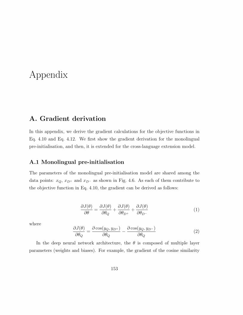
Appendix
A. Gradient derivation
In this appendix, we derive the gradient calculations for the objective functions in
Eq. 4.10 and Eq. 4.12. We first show the gradient derivation for the monolingual
pre-initialisation, and then, it is extended for the cross-language extension model.
A.1 Monolingual pre-initialisation
The parameters of the monolingual pre-initialisation model are shared among the
data points: xQ, xD+ and xD− as shown in Fig. 4.6. As each of them contribute to
the objective function in Eq. 4.10, the gradient can be derived as follows:
∂J(θ)
∂θ=∂J(θ)
∂θQ+∂J(θ)
∂θD+
+∂J(θ)
∂θD−(1)
where∂J(θ)
∂θQ=∂ cos(yQ, yD+)
∂θQ− ∂ cos(yQ, yD−)
∂θQ(2)
In the deep neural network architecture, the θ is composed of multiple layer
parameters (weights and biases). For example, the gradient of the cosine similarity
153
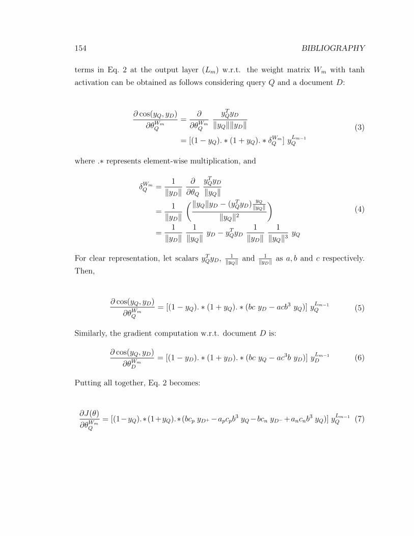
154 BIBLIOGRAPHY
terms in Eq. 2 at the output layer (Lm) w.r.t. the weight matrix Wm with tanh
activation can be obtained as follows considering query Q and a document D:
∂ cos(yQ, yD)
∂θWmQ
=∂
∂θWmQ
yTQyD
‖yQ‖‖yD‖= [(1− yQ). ∗ (1 + yQ). ∗ δWm
Q ] yLm−1
Q
(3)
where .∗ represents element-wise multiplication, and
δWmQ =
1
‖yD‖∂
∂θQ
yTQyD
‖yQ‖
=1
‖yD‖
(‖yQ‖yD − (yTQyD)yQ‖yQ‖
‖yQ‖2
)=
1
‖yD‖1
‖yQ‖yD − yTQyD
1
‖yD‖1
‖yQ‖3yQ
(4)
For clear representation, let scalars yTQyD, 1‖yQ‖
and 1‖yD‖
as a, b and c respectively.
Then,
∂ cos(yQ, yD)
∂θWmQ
= [(1− yQ). ∗ (1 + yQ). ∗ (bc yD − acb3 yQ)] yLm−1
Q (5)
Similarly, the gradient computation w.r.t. document D is:
∂ cos(yQ, yD)
∂θWmD
= [(1− yD). ∗ (1 + yD). ∗ (bc yQ − ac3b yD)] yLm−1
D (6)
Putting all together, Eq. 2 becomes:
∂J(θ)
∂θWmQ
= [(1−yQ).∗(1+yQ).∗(bcp yD+−apcpb3 yQ−bcn yD−+ancnb3 yQ)] y
Lm−1
Q (7)
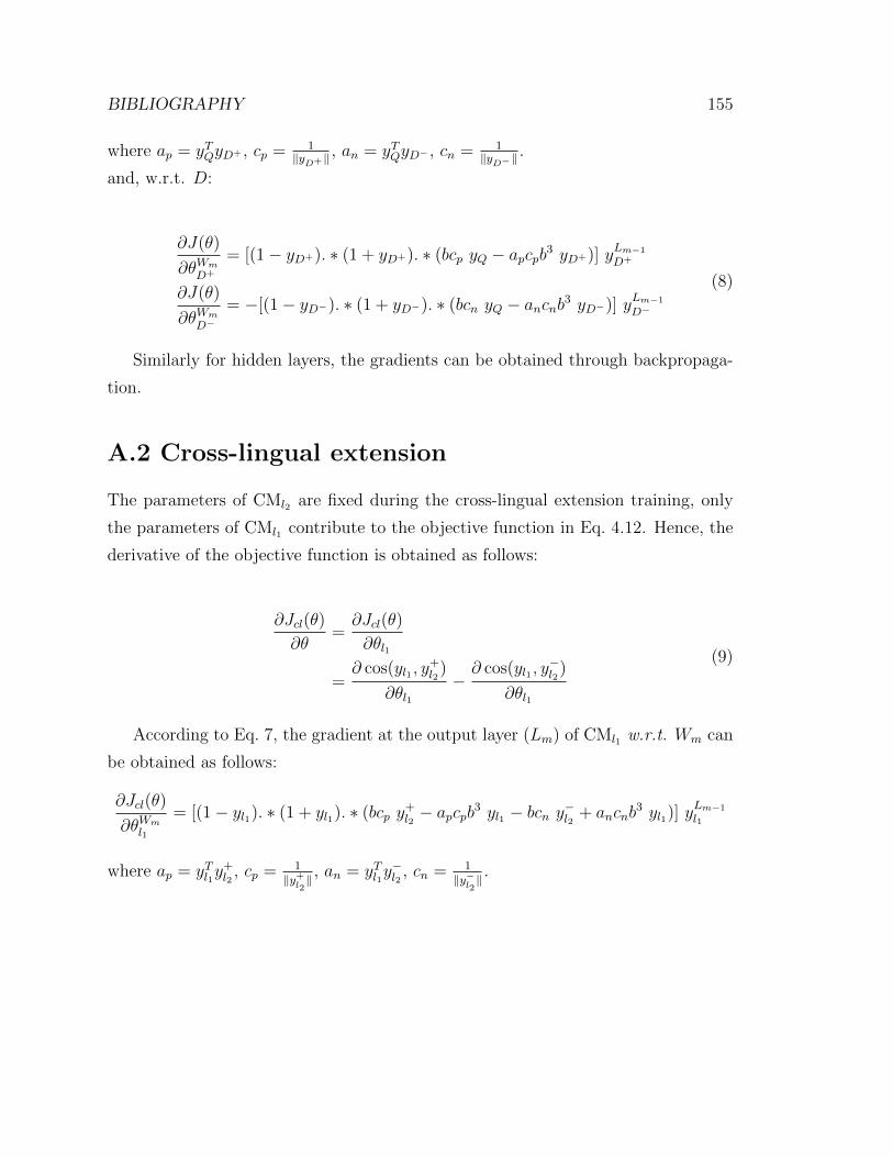
BIBLIOGRAPHY 155
where ap = yTQyD+ , cp = 1‖yD+‖ , an = yTQyD− , cn = 1
‖yD−‖.
and, w.r.t. D:
∂J(θ)
∂θWm
D+
= [(1− yD+). ∗ (1 + yD+). ∗ (bcp yQ − apcpb3 yD+)] yLm−1
D+
∂J(θ)
∂θWm
D−
= −[(1− yD−). ∗ (1 + yD−). ∗ (bcn yQ − ancnb3 yD−)] yLm−1
D−
(8)
Similarly for hidden layers, the gradients can be obtained through backpropaga-
tion.
A.2 Cross-lingual extension
The parameters of CMl2 are fixed during the cross-lingual extension training, only
the parameters of CMl1 contribute to the objective function in Eq. 4.12. Hence, the
derivative of the objective function is obtained as follows:
∂Jcl(θ)
∂θ=∂Jcl(θ)
∂θl1
=∂ cos(yl1 , y
+l2
)
∂θl1− ∂ cos(yl1 , y
−l2
)
∂θl1
(9)
According to Eq. 7, the gradient at the output layer (Lm) of CMl1 w.r.t. Wm can
be obtained as follows:
∂Jcl(θ)
∂θWml1
= [(1− yl1). ∗ (1 + yl1). ∗ (bcp y+l2− apcpb3 yl1 − bcn y−l2 + ancnb
3 yl1)] yLm−1
l1
where ap = yTl1y+l2
, cp = 1‖y+l2‖
, an = yTl1y−l2
, cn = 1‖y−l2‖
.
156 BIBLIOGRAPHY
B. Publications
The research presented in this dissertation has been published in many peer-reviewed
conferences and journals. The models, CAE and XCNN, presented in Chapter 4 are
published at (Gupta et al., 2014) and (Gupta et al., 2016a), respectively. The exper-
iments for CLIR applications presented in Chapter 6 are published at various places:
ad-hoc and parallel sentence retrieval tasks at (Gupta et al., 2016a), cross-language
plagiarism detection at (Barron-Cedeno et al., 2013; Franco-Salvador et al., 2013,
2016) and source context feature for machine translation at (Gupta et al., 2016b).
The research on mixed-script IR presented in Chapter 5 is published at Gupta et al.
(2014); Gupta (2014). The work on critical bottleneck dimensionality and related
metrics presented in Chapter 7 is published at (Gupta et al., 2016c).
The publications related to the work on this dissertation are listed below:
1. Gupta, P., Bali, K., Banchs, R. E., Choudhury, M., and Rosso, P. (2014).
Query expansion for mixed-script information retrieval. In Proceedings of the
37th International ACM SIGIR Conference on Research & Development in
Information Retrieval , SIGIR ’14, pages 677–686, New York, NY, USA. ACM
2. Gupta, P. (2014). Modelling of terms across scripts through autoencoders. In
Proceedings of the 37th International ACM SIGIR Conference on Research &
Development in Information Retrieval , SIGIR ’14, pages 1279–1279, New York,
NY, USA. ACM
3. Gupta, P., Banchs, R. E., and Rosso, P. (2016a). Continuous space models for
CLIR. Information Processing & Management , 53(2), 359–370
4. Gupta, P., Costa-Jussa, M. R., Rosso, P., and Banchs, R. E. (2016b). A deep
source-context feature for lexical selection in statistical machine translation.
Pattern Recognition Letters , 75, 24–29
5. Gupta, P., Banchs, R. E., and Rosso, P. (2016c). Squeezing bottlenecks: Ex-
BIBLIOGRAPHY 157
ploring the limits of autoencoder semantic representation capabilities. Neuro-
computing , 175, 1001–1008
6. Barron-Cedeno, A., Gupta, P., and Rosso, P. (2013). Methods for cross-
language plagiarism detection. Knowledge-Based Systems , 50, 211–217
7. Franco-Salvador, M., Gupta, P., and Rosso, P. (2013). Cross-language plagiar-
ism detection using a multilingual semantic network. In Proceedings of the 35th
European Conference on Advances in Information Retrieval , ECIR’13, pages
710–713, Berlin, Heidelberg. Springer-Verlag
8. Franco-Salvador, M., Gupta, P., Rosso, P., and Banchs, R. E. (2016). Cross-
language plagiarism detection over continuous-space- and knowledge graph-
based representations of language. Knowledge-Based Systems , 111, 87–98
9. Gupta, P., Rosso, P., and Banchs, R. E. (2013a). Encoding transliteration vari-
ation through dimensionality reduction: FIRE Shared Task on Transliterated
Search. In Fifth Forum for Information Retrieval Evaluation, FIRE ’13
10. Costa-jussa, M. R., Gupta, P., Rosso, P., and Banchs, R. E. (2014). English-
to-hindi system description for WMT 2014: Deep source-context features for
Moses. In Proceedings of the Ninth Workshop on Statistical Machine Trans-
lation, WMT ’14, pages 79–83, Baltimore, Maryland, USA. Association for
Computational Linguistics
The publications that are partially related to the dissertation and obtained during
the course of the PhD are listed below:
1. Sequiera, R., Choudhury, M., Gupta, P., Rosso, P., Kumar, S., Banerjee, S.,
Naskar, S. K., Bandyopadhyay, S., Chittaranjan, G., Das, A., and Chakma,
K. (2015). Overview of FIRE-2015 shared task on mixed script information
retrieval. In Seventh Forum for Information Retrieval Evaluation, FIRE ’15,
pages 19–25
158 BIBLIOGRAPHY
2. Dubey, A., Gupta, P., Varma, V., and Rosso, P. (2014). Enrichment of bilingual
dictionary through news stream data. In Proceedings of the Ninth International
Conference on Language Resources and Evaluation, LREC ’14, pages 3761–
3765
3. Choudhury, M., Chittaranjan, G., Gupta, P., and Das, A. (2014). Overview
of FIRE 2014 track on transliterated search. In Sixth Forum for Information
Retrieval Evaluation, FIRE ’14
4. Gupta, P., Clough, P. D., Rosso, P., Stevenson, M., and Banchs, R. E. (2013b).
PAN@FIRE: Overview of the Cross-Language !ndian News Story Search (CL!NSS)
track. In Fifth Forum for Information Retrieval Evaluation, FIRE ’13
5. Gupta, P. and Rosso, P. (2012a). Expected divergence based feature selection
for learning to rank. In Proceedings of the 24th International Conference on
Computational Linguistics , COLING ’12, pages 431–440
6. Gupta, P. and Rosso, P. (2012b). Text reuse with ACL: (Upward) Trends.
In Proceedings of the ACL-2012 Special Workshop on Rediscovering 50 Years
of Discoveries , ACL ’12, pages 76–82, Stroudsburg, PA, USA. Association for
Computational Linguistics
7. Gupta, P., Barron-Cedeno, A., and Rosso, P. (2012b). Cross-language high
similarity search using a conceptual thesaurus. In Proceedings of the Third
International Conference on Information Access Evaluation: Multilinguality,
Multimodality, and Visual Analytics , CLEF ’12, pages 67–75, Berlin, Heidel-
berg. Springer-Verlag
8. Potthast, M., Gollub, T., Hagen, M., Kiesel, J., Michel, M., Oberlander, A.,
Tippmann, M., Barron-Cedeno, A., Gupta, P., Rosso, P., and Stein, B. (2012).
Overview of the 4th international competition on plagiarism detection. In
CLEF Evaluation Labs and Workshop, Online Working Notes , CLEF ’12


![Neural Graph Collaborative Filtering · 2019-05-21 · item embeddings]. (1) It is worth noting that this embedding table serves as an initial state for user embeddings and item embeddings,](https://static.fdocuments.in/doc/165x107/5e4b2359136a851cfe576dbe/neural-graph-collaborative-filtering-2019-05-21-item-embeddings-1-it-is-worth.jpg)