Cross Hedging with Single Stock Futures

17 December 2004

§ C.Brooks@city.ac.uk (Corresponding Author)

Chris Brooks§

Faculty of Finance Cass Business School

City University 106 Bunhill Row

London, EC1Y 8TZ UK

Ryan J. Davies

Finance Division Babson College Tomasso Hall

Babson Park, MA 02457 USA

Sang Soo Kim

ISMA Centre University of Reading

PO Box 242 Whiteknights

Reading RG6 6BA UK

Cross Hedging with Single Stock Futures

Abstract

This study evaluates the efficiency of cross hedging with the new single stock futures (SSF) contracts recently introduced in the United States. We use matched sample estimation techniques to select SSF contracts that will reduce the basis risk of cross hedging and will yield the most efficient hedging portfolio. By employing multivariate matching techniques with cross-sectional matching characteristics, we can considerably improve hedging efficiency relative to the use of return correlations alone. Overall, we find that the best hedging performance is achieved through a portfolio that is hedged with market index futures and a SSF matched by both historical return correlation and cross-sectional matching characteristics. We also find it preferable to retain the chosen SSF contracts for the whole out-of-sample period but to re-estimate the optimal hedge ratio for each rolling window.

1

1 Introduction There are a variety of reasons why investors, particularly individuals, may

have substantial undiversified exposures to single stocks. For example, an investment bank that acquires shares of a firm through syndication may be subject to a covenant that restricts the sale of these shares. Similarly, an investor may hold stock options that are currently deep in the money but for which selling is not permitted for a prescribed period. Or, a fund manager may also have a large exposure to a stock that for some reason he does not want to close out. In all of these cases, the investor may desire hedging to protect against price falls rather than selling.

One way that an investor could deal with such a problem is to enter into an

offsetting short position. This position’s associated costs, such as margin requirements, up-tick trading restrictions, and loan interest, mean that it is likely to be a high cost tool. As another alternative, the investor could consider listed stock options. This may not be practical, however, since of the 7500 stocks listed on the three major U.S. stock exchanges, 5300 do not have listed options written on them. Over-the-counter options have substantial initial premiums and are often priced using opaque “black box” methods.

Futures contracts are likely to represent a much cleaner hedging tool.

Futures contracts have no premium, low transaction costs, low margin requirements, and more transparent pricing than over-the-counter options. Hedging with stock index futures is certainly easy and cost-effective, but may provide an inadequate hedge if the returns profile of the stock exposure is significantly different to that of the index as a whole. Alternatively, one may consider hedging with single stock futures (SSF) contracts. Such a hedge is likely to work well if there is a traded future on the required stock. In cases where the required SSF does not exist, the investor faces a choice: hedge with a stock index or cross-hedge using the futures contract of a closely related stock. Since cross-hedging efficiency is sometimes degraded by the inevitable ‘basis risk’, it is essential to select the appropriate futures contract carefully and to develop an effective cross-hedging model.

To this end, the objective of this study is to evaluate the efficiency of cross

hedging with the new SSF contracts introduced in the U.S. market in November 2002. At the end of August 2004, there were futures on 116 individual U.S.

2

stocks. To cross hedge other stocks, we propose using a matching technique that matches the spot stock with one or more of the available SSF contracts in a manner designed to reduce the basis risk of cross hedging and to obtain the most efficient hedging portfolio.

While there has been extensive testing of the various econometric models

available to estimate the optimal hedge ratio, there has been little research concerning how to select optimally the hedging asset which minimizes the basis risk of cross hedging. If the futures contract for the specific individual stock does not exist, the effectiveness of the hedge may depend more crucially on the selected futures contract than on the optimality of the estimated hedge ratio.

The hedging efficiency of conventional models for estimating the optimal

hedge ratio depends on the return covariance between the spot and hedging assets. As the estimated hedge ratio and resulting efficiency are contingent on the sample period and its length, there is no guarantee that an effective hedge will continue over a different time horizon. Unfortunately, there is no universally accepted objective criterion to decide the appropriate length of the sample period.

As an alternative, one could consider the common fundamental factors that

affect the price movement of the spot asset and the hedging asset. In the context of cross hedging, if two assets have similar fundamental factors that determine their subsequent price movements, then the resulting hedge can be expected to be relatively effective. We propose matching the spot asset with the ideal hedging asset(s) using nonparametric sample matching techniques that control those fundamental factors as the matching characteristics. The resulting hedged portfolio should minimize the basis risk. We show that using matching techniques to construct the hedged portfolio can provide efficiency gains over a hedged portfolio constructed purely according to the correlation between the futures and spot returns.

For the empirical analysis, we construct four types of cross-hedged portfolios that are hedged with: i) single SSF only, ii) single SSF and market index futures, iii) multiple SSF contracts, and iv) multiple SSF contracts and market index futures. Each futures contract is chosen by sample matching techniques using three different matching characteristic sets. The first matching characteristic set consists of only historical return correlations between spot and

3

potential futures implied in the conventional cross hedging model. The second set consists of possible fundamental factors that influence the price movements of stocks. The last set includes both return correlations and fundamental factors. Finally, we repeat the same analysis with the additional restriction that the selected SSF contracts are from the same industry as the spot stock.

To examine the hedging efficiency of each hedged portfolio, we consider the

percentage reduction of the variance of the hedged portfolio relative to that of the unhedged portfolio as the first criterion. The second criterion is the reduction in the mean of the negative payoffs of the hedged portfolio, since the purpose of hedging is often the elimination of downside price risk. To estimate the hedging efficiency of each model over time, we construct a hedged portfolio with a 1-day life and roll it over with fixed sized windows. Furthermore, as our purpose is not the investigation of the fitness of the model in-sample, the hedging performance is examined out-of-sample.

The remainder of this paper is organised as follows. Section 2 summarizes

the SSF markets. Section 3 outlines the methodology employed for estimating the hedge ratio and determining hedging efficiency. Section 4 outlines the various cross-hedging models based on different hedging strategies, while Section 5 describes data. Section 6 explains the estimation procedure and rebalancing methods. Section 7 presents the estimation results and finally, Section 8 concludes and makes suggestions for further study.

2 Cross-Hedging and the Single Stock Futures Market The benefits of hedging with futures have been well studied, and cross hedging with futures has been successfully used in various financial markets including commodity, foreign exchange and stock markets. For example, Brooks and Chong (2001) compare the efficiency of cross-hedging in foreign currency markets. Foster and Whiteman (2002) investigate the cross-hedging efficiency of spot soybeans that have a different harvesting location from the futures commodity. Franken and Parcell (2003) examine the hedging efficiency of spot ethanol with NYMEX unleaded gasoline for multiple period hedging.

Both market players and academics have recognised the potential benefits of single stock futures. These benefits include: (i) SSFs enable easy short selling; (ii) SSFs reduce the cost of obtaining a leveraged long position; (iii) SSFs

4

provide the opportunity for spread trading; (iv) SSFs enable a trader to isolate a stock from an index; and (v) SSFs provide a cleaner and more efficient hedging tool than options. Despite these benefits, SSFs have only recently been introduced. Outside of the U.S., SSFs are now traded on the futures exchanges of Hong Kong, London, Madrid, Warsaw, Helsinki, South Africa, Mexico and Bombay, among others (see Lascelles (2002) for a survey of exchanges trading SSF contracts in April 2001). As a result of their lack of history, SSFs have been subject to very little attention in published research. Exceptions include Dutt and Wein (2003), who suggest appropriate margin requirements for the U.S. SSF market, and McKenzie, Brailford and Faff (2001), who investigate the impact of SSF listing on the liquidity of the spot stock market in Australia.1

In Europe, the London International Financial Futures and Options Exchange (LIFFE)2 began trading 25 Universal Stock Futures – its brand name corresponding to SSF – with cash settlement on January 29, 2001 and launched physical delivery contracts on November 21, 2002. LIFFE runs a central order book with a fully electronic system and listed 141 SSFs from 12 different countries in August 2004. Its year-to-date volume of over 11 million (124% year-on-year growth) makes it the world’s largest SSF exchange in terms of trading volume. However, we focus on U.S. SSF markets in our empirical analysis to avoid complications arising from trading across time zones, and to avoid any country effects.

Prior to November 2002, SSF contracts were not permitted in the U.S. In

part, this was because of regulatory concerns about the leverage effect of SSF and possible manipulation of the underlying spot stock price. The approval of listing standards and margin requirements by the Securities and Exchange Commission and the authorization of trading rules by the Commodity Futures Trading Commission paved the way for the launch of the first U.S.-based SSF markets: OneChicago and Nasdaq.LIFFE.

OneChicago launched a SSF market on November 8, 2002 with 21 SSFs. At

the end of August 2004, open interest stood at 134,997 contracts and the number

1 See also Ang and Cheng (2004a, 2004b), Hung, Lee, and So (2003), and Partnoy (2001). 2 Following the purchase of LIFFE by Euronext in 2001, LIFFE became part of Euronext.LIFFE, comprising of the Amsterdam, Brussels, LIFFE, Lisbon, and Paris derivative markets. LIFFE still has over 90% of the trading volume among the five derivatives exchanges of Euronext.LIFFE.

5

of listed SSFs was 119. Their recorded year-to-date volume in August 2004 was 1,172,998 contracts, 33% greater than 2003. The average daily volume was 3,158 contracts in August 2004. Since it is a joint venture of the Chicago Board Options Exchange, the Chicago Mercantile Exchange, and the Chicago Board of Trade, it adopted a market maker system in accordance with its mother companies, the so-called Lead Market Maker who quotes continuous two-sided prices and ensures liquidity.

Nasdaq.LIFFE (NQLX), a wholly owned subsidiary of Euronext.LIFFE, was also launched with 10 SSFs on the same day as OneChicago. At the end of August 2003, open interest stood at 37,434 contracts and the number of listed SSFs was 58. It traded 65,569 contracts in June 2004. Instead of the single market maker system of OneChicago, it adopted a multiple market-making firms system, giving them several incentives. Each must compete against other market makers and public customers for every single order, since NQLX combines the market maker system with a central order book system.

3 Methodology 3.1 Cross hedging and Basis Risk

In fact, hedging using futures is often a cross hedging of sorts because the quality and/or the quantity of the underlying spot assets usually differ from those of the futures contracts used for hedging. As a result of these differences, cross hedging inevitably causes basis risk - that is, a difference in price between the spot and futures at maturity. Therefore, minimizing basis risk is the most important criterion for improving cross-hedging efficiency.

Following Hull (2002), the payoff of a hedged portfolio with hedge ratio 1 can be written

TFTFTS PPP ,1,, −+ − (1)

where PS indicates the price of the spot asset, and PF indicates the price of the futures contract. At time T-1, the hedge is put in place, and at time T, the hedging position is closed.

When we consider cross hedging, equation (1) can be rewritten

)()( *,,,

*,1, TSTSTFTSTF PPPPP −+−+− (2)

6

where the superscript * indicates that the underlying asset of the hedging futures is different from the spot asset exposed. Equation (2) illustrates that the basis from cross hedging consists of two components. The first component, P*S,T – PF,T, represents the basis risk from the difference in price at clearing time between the futures and the spot asset, given that the spot is the same as the underlying asset of the futures contract. The second component, PS,T – P*S,T, captures the difference between the spot and the underlying asset of the futures contract. Since the first component of the basis risk cannot be controlled, the main concern in cross hedging is the minimization of the second component of the basis risk. That means that we have to select the ‘optimal futures’ whose underlying asset has the most similar price movement to that of the spot asset.

3.2 The Optimal Hedge Ratio

When the hedge ratio is defined as the ratio of the futures exposure to the spot exposure, the naive hedge ratio with a value of -1 is only optimal when the spot and futures returns are perfectly correlated and constant over time. Clearly, this is not supported empirically. The key, therefore, is to estimate the ‘optimal’ hedge ratio. As Lien and Tse (2002) review and summarize, we can categorize the models for estimating the optimal hedge ratio by the purpose of hedging, including the asset manager’s behavior through his utility function, and the assumptions for the joint probability distribution of the futures and spot returns. The OLS Hedge Ratio The optimal hedge ratio that minimizes the variance of the payoff of the hedged portfolio is analytically the same as the slope coefficient of a regression of the spot on the futures returns. Ederington (1979) shows that the optimal hedge ratio to minimize the variance of the payoff of the hedged portfolio usually differs from 1. Anderson and Danthine (1980) extend the analysis to multiple hedging futures by considering the degree of risk aversion in the utility function, and prove that the optimal hedge ratio for each futures asset is analytically the same as the slope coefficients of each futures asset in a multiple regression. Thus, the optimal hedge ratio for hedging with a single futures asset can be estimated by following the ordinary least squares (OLS) method,

ttFOLStS rHRr εα +⋅+= ,, (3)

where rt are the returns and εt is a white noise error term. HROLS and α are the regression parameters. The coefficient of multiple determination from this regression, R2, represents the in-sample hedging efficiency.

7

The optimal hedge ratio (HROLS) can also be expressed as

F

FS

F

SFSOLSHR

σσ

σσ

ρ == (4)

where ρFS is the correlation between spot and futures returns, σF is the standard deviation of futures returns, and σFS is the covariance between the spot and futures returns.

Comparing equations (2) and (3), the error term of equation (3) represents

the sum of the basis risk components of equation (2). Thus, the minimization of the basis risk of equation (2) is equivalent to the minimization of the variance of the error term of equation (3), or maximization of R2 for that regression. If the underlying of the futures asset is exactly the same as the spot asset, the correlation is likely to be near its maximum possible value of unity, and the hedging efficiency of the OLS model would be guaranteed if the correlation is constant over time and the amount of the spot asset is deterministic.

Other Approaches to Estimating the Hedge Ratio More recently, researchers developed a method for maximizing the expected utility function taking account of the mean-variance of the hedged portfolio payoff. This means that the optimal hedge ratio must make the hedger’s subjective marginal substitution ratio between risk and returns equal to that of the objective hedged portfolio. Anderson and Danthine (1981) 3 prove that the optimal hedge ratio in a mean-variance context for the pure hedger is equal to the variance minimizing hedging ratio with predetermined spot position when the futures price follows a martingale (i.e. E(∆F)=0). Cecchetitti, Cumby and Fieglewski (1988) argue, through an empirical analysis of the U.S. Treasury bond market, that the optimal hedge ratio to maximize a log utility function is smaller than the risk-minimizing ratio.

An alternative approach to the estimation of the optimal hedge ratio is

derived from the time varying variance of futures returns and covariance between spot and futures returns. Since econometric models such as the GARCH model have been adopted to capture the time varying second moment of returns distributions, many academics have used them to estimate a dynamic

3 They derive the optimal hedge ratio for cross hedging by maximizing a utility function which is an increasing function of the expected return of the hedged portfolio and a decreasing function of the variance of it and of risk aversion.

8

optimal hedge ratio allowing for time varying variances and covariances of the joint probability distribution.

Baillie and Myers (1991) apply the bivariate GARCH model to data from the commodity futures market, and argue that a time-invariant (OLS) hedge ratio is inappropriate and that a GARCH model performs better than the regression model, especially out-of-sample. Kroner and Sultan (1993) adopt a bivariate constant correlation GARCH model for the foreign currency market with an error correction specification in the mean equation. Brooks, Henry and Persand (2002) extend their framework by employing an asymmetric multivariate GARCH model for the relationship between stock index and stock index futures returns. Brooks and Chong (2001) compare the cross hedging efficiency in the foreign currency market between 11 models, including seven from the GARCH family. The latter conclude that simple EWMA (Exponentially Weighted Moving Average) model produces the lowest variance, arguing the simple model is better able to generalize and is not over-fitted to the data. Poomimars, Cadle and Thebald (2003) smooth the volatile dynamic hedge ratio from a GARCH model by adding a constant hedging ratio.

However, all of the above models, including the OLS hedge ratio, assume either that the best futures asset is optimally given to minimize the second component of equation (2) for cross hedging or that the hedging futures’ underlying asset exists in the spot market. There is no literature providing a theoretical method to minimize the second component of equation (2) or examining its effect on basis risk – and therefore, on hedging efficiency.

We develop a hedging model that reduces basis risk by selecting an optimal hedging futures asset as well as estimating the optimal hedge ratio. We adopt the variance minimizing hedge ratio estimated using OLS because a comparison of the efficiency of the hedge ratio is not the main focus of this paper. Empirically, it has been shown that there is often little difference in out-of-sample hedging efficiency between hedge ratios estimated using OLS and with other more complex models – see, for example, Brooks et al. (2002). Moreover, in practice, the OLS hedge ratio is widely used by market players thanks to its simplicity of understanding and estimation.

3.3 Hedging Efficiency

The measure most commonly used to gauge hedging efficiency in the futures

9

literature is related to the variance of the payoff of the hedged portfolio - either the level of the variance or the reduction ratio to that of an unhedged portfolio. This means that the smaller variance of the hedged portfolio, the larger the probability that it has a lower basis risk. It is worth noting that the hedge ratio from a parametric regression model analytically guarantees the minimum variance in-sample providing that the hedging futures series employed has the highest correlation with the spot asset during the in-sample period.

The payoff of the hedged portfolio p is defined as

∑ ∑ ⋅−⋅=i j

Fjj

Siip rHRrwHP )( (5)

where riS is the return of individual spot asset i, rjF is the return of hedging futures j, HRj is the hedge ratio for futures j estimated by OLS, and wi are the weightings of the spot assets.

For comparison, we use the percentage reduction in variance of various

hedged portfolios against that of an unhedged portfolio. Therefore, the percentage reduction in the variance of the payoff for portfolio p is

( )( ) 100)()(1 ,,, ×−= UNpSMpSMp HPVarHPVarVR (6)

where Var represents the payoff variance of portfolio p during the out-of-sample period, SM denotes each type of hedging model and UN is the unhedged case.

The second criterion employed in this paper for judging hedging efficiency

is the mean of the negative payoffs of the hedged portfolio, which is defined as

∑∑==

⋅=T

tt

T

tttp DDHPNEG

11

(7)

where T is the end date of out-of-sample period, Dt is equal to 1 when HPt <0, and 0 otherwise. For comparison between hedging models, we use the percentage reduction in the mean daily negative payoff against that of an unhedged portfolio. Therefore, the percentage reduction in the mean of negative payoffs is

( ) 100)(1 ,, ×−= UNpSMpp NEGNEGNR . (8)

It may also be the case that the purpose of hedging is the maximization of the expected return of the hedged portfolio given a particular tolerable risk level of the hedger. However, some academics have recently argued for an

10

asymmetric impact of hedged portfolio returns on the utility of a pure hedger. This means that a loss has a larger negative impact on utility than the positive impact of an equally sized gain. Under the notion of loss aversion, Lien (2001a) shows using a constant absolute risk aversion utility function that the effect of loss aversion on futures hedging exists only in the backwardation or contango cases. Lien (2001b) suggests that disappointment aversion discourages the hedger from deviating from the fully hedged position. However, as the degree of risk aversion is usually unobservable and given the abstract nature of the utility function framework, we instead examine the mean of the actual negative payoffs that the hedger tries to eliminate by constructing the hedged portfolio.

4 A Cross Hedging Model with Matched SSF Contracts It is common to choose the futures asset for cross hedging based on only the

historical return correlation, ρ, since the highest historical return correlation ensures the highest historical hedging efficiency (i.e. the minimum variance of the hedged portfolio payoff) during the in-sample period. However, as discussed above, this may not provide optimal out-of-sample performance.

From another viewpoint, if two assets have similar fundamental factors that

affect their future price movements, we may expect that the price movements between these two assets would also be similar. Thus, we may consider the common fundamental factors that could affect the price movement of the spot and hedging assets. We may obtain a more appropriate cross hedging instrument via a consideration of fundamental factors rather than return correlations since the latter are likely to be considerably noisier than the former. Return correlations are also likely to be unstable, varying more from one sample to another through time than fundamentals.

Using a sample matching technique, we can select the most appropriate proxy

for a particular object in terms of its matching characteristics. If we use those fundamental factors as the matching characteristics, and choose the futures asset as a proxy whose underlying asset has the closest characteristics to the spot asset, we may expect that the price movement of the selected proxy futures asset can be similar to that of the spot asset that we wish to hedge. Also, as sample matching techniques use cross-sectional information, they do not depend on the specific sample period or its length. Each of following subsections present the different hedging models based on using different

11

matching characteristics and techniques.

4.1 Matching Characteristics We construct three sets of matching characteristics (X). The first set consists

of only the historical return correlation. The second consists of only the fundamental factors, which are earnings per share, capital asset pricing model (CAPM) beta and market capitalization. The final set consists of both the correlation and the fundamental factors. For multiple matching characteristics, we measure the distance between spot and hedging futures, in terms of matching characteristics, using the Mahalanobis metric:

)()(|||| 1FSFSFS XXSXXXX −′−=− − (9)

where FFSS SNSNS )1()1( −+−= , ND denotes the sample size, and SD denotes the sample covariance for D=S, F. Given each set of matching characteristics, for each spot asset, we select the futures contract(s) which minimize(s) the distance in equation (9) as the corresponding hedging futures.

4.2 Industry Classification It is likely that, all other things being equal, firms within the same industry

will have stock price movements that are more correlated than they are with those in other industries. This suggests that the hedger may primarily seek a hedging SSF that is in the same industry sector as the spot asset to minimize the industry effect. Hence, we examine whether classification of futures by industry can help to improve cross-hedging efficiency. The SSF contracts and spot stocks are classified according to their FTSE “level 3” economic and industrial sector, and then spot stocks are matched with SSF contracts within the same industrial classification. We use the lowest level of FTSE industry classification to ensure there is always a SSF to match with each spot stock.

4.3 Hedging with multiple matched SSF contracts In the context of currency futures, DeMaskey (1997) shows that hedging

with multiple futures contracts performs better than hedging with a single futures contract. Furthermore, he finds that adding more than three futures is unlikely to improve performance further. In light of these results, it is reasonable to suppose that using multiple SSF contracts to hedge could result in better hedging efficiency relative to that of using a single SSF. We explore this possibility by using up to three SSF contracts of “nearby” stocks to hedge.

12

4.4 Hedging with SSF contracts and Market Index Futures Hedging with market index futures is the most prevalent hedging tool for

spot stocks having no derivatives, since it allows for a diversified portfolio to eliminate market risk with low trading costs. However, as index futures can only eliminate market risk, the residual basis risk could be substantial. In other words, index futures cannot remove firm specific risk. Therefore, if we hedge the spot stocks’ exposures with market index futures in addition to the matched individual stock futures, the hedging efficiency may improve because this approach may mitigate both the market risk and the residual firm specific risk.

Thus, to summarize, we have with four types of cross-hedged models,

hedged with: i) single matched futures only; ii) single matched futures and market index futures; iii) multiple futures; and iv) multiple futures and market index futures. The hedging SSF contracts are matched by: i) return correlation only; ii) cross-sectional fundamental factors only; and iii) both of them. All models are examined both with and without industrial classification.

5 Data The focus of our empirical analysis is the equity spot market and the SSF

market in the U.S. To ensure a sufficient number of observations to estimate the return correlations, we restrict our sample to SSF contracts that were listed before September 12, 2003. For 51 SSF contracts that are listed on more than one exchange, we select the more liquid OneChicago market. Our final sample of 97 SSFs consists of 90 from OneChicago and 7 from NQLX. We have excluded 26 SSF contracts of OneChicago that were listed after June 2004, and 3 SSF contracts of OneChicago that are non-standard listings.

The sample period runs from September 12, 2003 to August 31, 2004, which

corresponds to the listing period of our 97 SSF contracts. We collect daily settlement prices of SSF contracts announced from OneChicago’s website, and those of Nasdaq.LIFFE are collected from its ‘pa’ files of the CBOE for settlement. To calculate the single price series for each SSF, we take an average of the prices of those contracts that are available at each date. S&P 500 index futures are used to represent the market index futures, and its price series over the sample period is obtained from the Datastream.

The criteria for the spot stocks included in our sample are that they must: i)

13

not have corresponding derivatives - either SSF or options4; ii) be firms based in the US to avoid non-synchronous trading or country effects; iii) have a market capitalization over $500 million at April 2004 to eliminate small firm and non-trading effects; iv) be listed on a U.S.-based stock exchange before September 12, 2003; and v) have matching characteristic data available. For the 438 stocks satisfying all five criteria, daily closing prices are collected from Datastream.

6 Estimation and Rebalancing To determine the ex-ante hedging efficiency during the out-of-sample period, rolling windows of fixed length (1-day), corresponding to the supposed portfolio life, are employed until data are exhausted. The issue of the lengths of the in-sample and out-of-sample periods will be discussed subsequently. Hedging efficiency is calculated using equations (6) and (8) – the variance reduction and the reduction in the mean of the negative payoffs respectively – assuming that each portfolio consists of one spot stock. Then, the hedging efficiency is estimated over the 438 spot stocks.

Assuming a short hedge and using the minimum-variance hedging ratios estimated by OLS in equation (4), we consider three rebalancing procedures for hedging efficiency. These three procedures impose different computation and transaction costs on the hedger and allow us to test whether increased hedging efficiency can be obtained by increasing the frequency of rebalancing.

Our first rebalancing procedure retains a single optimally chosen hedging

SSF contract for a given spot stock position and uses the same OLS hedge ratio over all rolling windows during the out-of-sample period. That is, there is a one-time matching and a one-time estimation of the hedge ratio at the start of the out-of-sample period, reflecting the least effort for the hedger and minimal transaction costs.

Our second rebalancing procedure fixes throughout the optimally chosen

SSF contracts for a given stock, but re-estimates the OLS hedge ratio at every rolling window during the out-of-sample period as new price information becomes available. This strategy reflects a medium level of effort on the part of the hedger and medium level transaction costs. 4 We employ this restriction so that hedging with the same futures asset as the underlying spot asset is not a possibility for any of the stocks in our sample.

14

Our last rebalancing procedure optimally re-selects, at each rolling window,

the hedging SSF contracts for each spot stock according to the new information, and re-estimates the hedge ratios. This procedure implies the heaviest burden of calculation for the hedger and the largest transaction costs. Note that the second and third methods both allow for the possibility of time-variation in the correlation between SSF and spot asset returns.

7 Results 7.1 Choice of Rebalancing Methods and Out-of-Sample Period

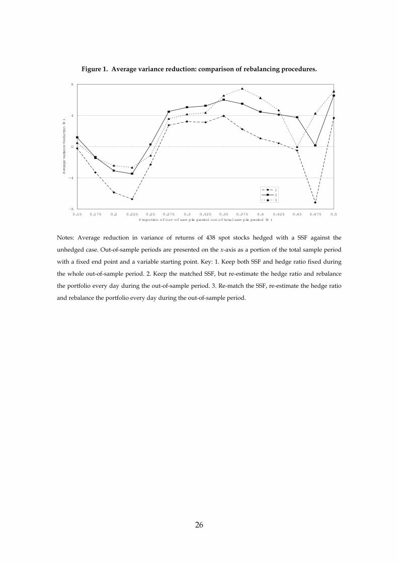
Before presenting the estimation results of different hedging models and different methods for choosing hedging SSF contracts, we examine in Figure 1 the issue of which rebalancing procedure shows the best hedging efficiency during the out-of-sample period. In Figure 1, the average variance reductions from different rebalancing methods are depicted over different lengths of out-of-sample period. Interestingly, our expectation that the most complicated rebalancing method would show the best performance is not supported. All three rebalancing methods are based on a hedge using a sole SSF matched by historical correlation only. Even though rebalancing according to the time varying hedge ratio performs better than the constant hedge ratio over the out-of-sample period, changing the SSF used for hedging according to the updated historical return correlation does not guarantee a better performance.

We have tested a total of 33 cases of hedging models – for example, hedging

with multiple SSF contracts, matching SSF contracts with different matching characteristic sets, adding industrial classifications, and with market index futures. Even though Figure 1 is based on the simplest hedging model, for most of the 33 hedging models, the second rebalancing procedure – re-estimating the hedge ratio and not re-selecting the SSF – is still preferred. Qualitatively identical results are also obtained for the second hedging efficiency criterion – the mean negative payoff. Therefore, the following sections focus on the results obtained from this second balancing method (that is, updating the hedge ratio but using the same SSF for a given stock for the whole out of sample period).

When conducting an out-of-sample evaluation of hedging efficiency, it is of

interest to examine the sensitivity of the results to the portion of the total sample that is retained as the out-of-sample period. To this end, we conduct all

15

estimation procedures for out-of-sample periods ranging from 15% to 50% of the total sample period. In Figure 1, for out-of-sample periods that constitute up to 28% or over 43% of the total sample, the evaluation of hedging efficiency is highly unstable. Thus, we choose 35% of the total sample for the out-of-sample period, which is the middle of the stable range, and which also ties in with the loose “two-thirds, one-third” rule commonly used in empirical analysis.

7.2 Matching characteristics

We examine the effect of three different matching characteristics on the choice of optimal hedging asset. The first one consists of the historical return correlation only while the second consists of four cross-sectional matching characteristics (earnings per share, capital asset pricing model beta and market capitalization). Both the historical correlation and the cross-sectional matching characteristics are combined in the last set.

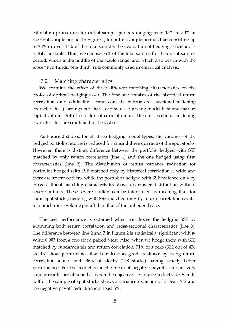
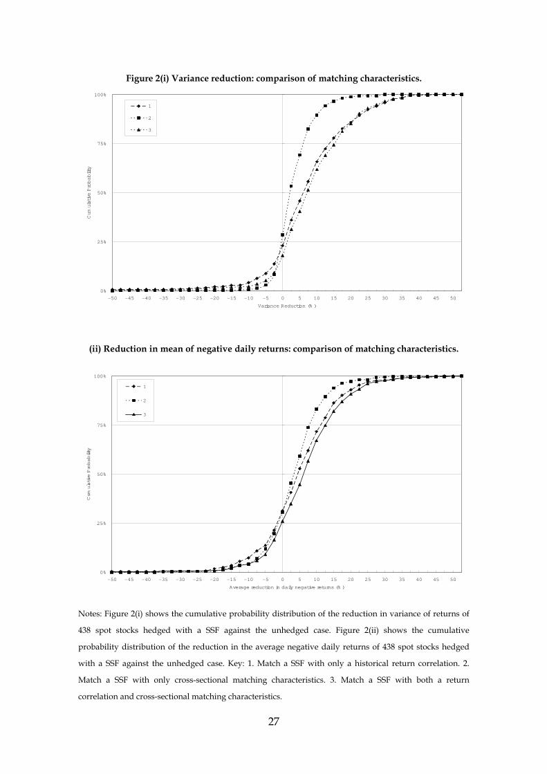
As Figure 2 shows, for all three hedging model types, the variance of the hedged portfolio returns is reduced for around three quarters of the spot stocks. However, there is distinct difference between the portfolio hedged with SSF matched by only return correlation (line 1) and the one hedged using firm characteristics (line 2). The distribution of return variance reduction for portfolios hedged with SSF matched only by historical correlation is wide and there are severe outliers, while the portfolios hedged with SSF matched only by cross-sectional matching characteristics show a narrower distribution without severe outliers. These severe outliers can be interpreted as meaning that, for some spot stocks, hedging with SSF matched only by return correlation results in a much more volatile payoff than that of the unhedged case.

The best performance is obtained when we choose the hedging SSF by

examining both return correlation and cross-sectional characteristics (line 3). The difference between line 2 and 3 in Figure 2 is statistically significant with p-value 0.003 from a one-sided paired t-test. Also, when we hedge them with SSF matched by fundamentals and return correlation, 71% of stocks (312 out of 438 stocks) show performance that is at least as good as shown by using return correlation alone, with 36% of stocks (158 stocks) having strictly better performance. For the reduction in the mean of negative payoff criterion, very similar results are obtained as when the objective is variance reduction. Overall, half of the sample of spot stocks shows a variance reduction of at least 7% and the negative payoff reduction is at least 6%.

16

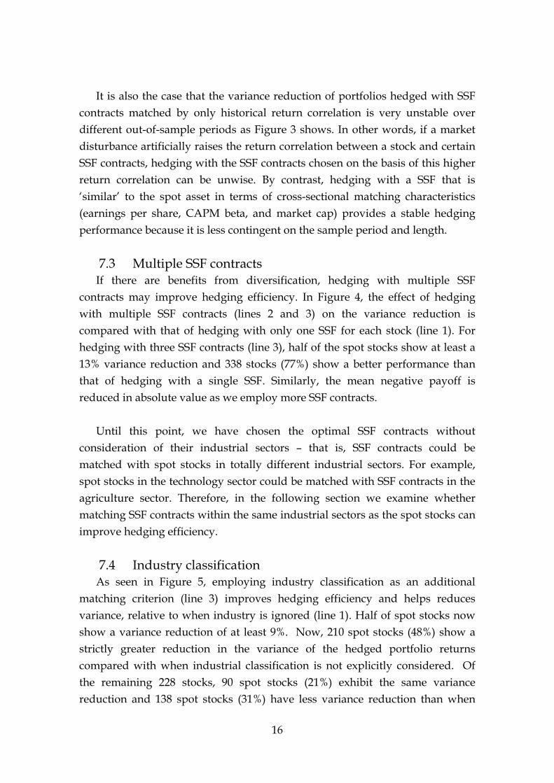
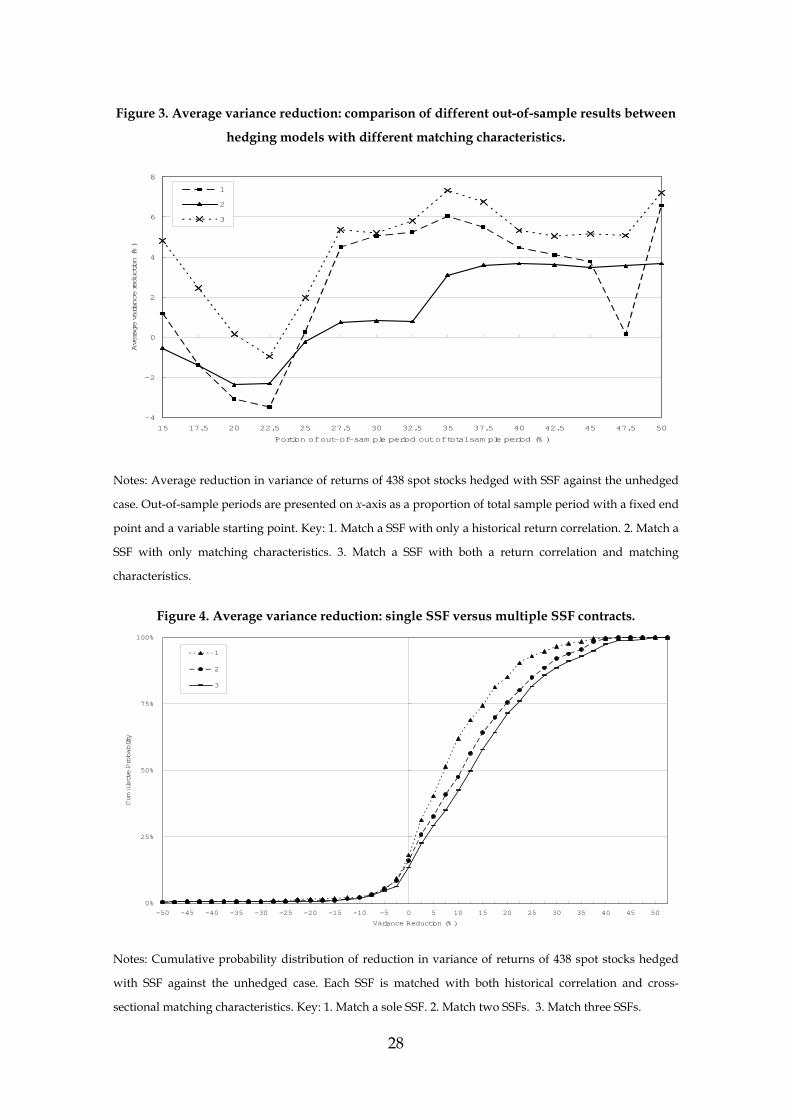
It is also the case that the variance reduction of portfolios hedged with SSF

contracts matched by only historical return correlation is very unstable over different out-of-sample periods as Figure 3 shows. In other words, if a market disturbance artificially raises the return correlation between a stock and certain SSF contracts, hedging with the SSF contracts chosen on the basis of this higher return correlation can be unwise. By contrast, hedging with a SSF that is ‘similar’ to the spot asset in terms of cross-sectional matching characteristics (earnings per share, CAPM beta, and market cap) provides a stable hedging performance because it is less contingent on the sample period and length.

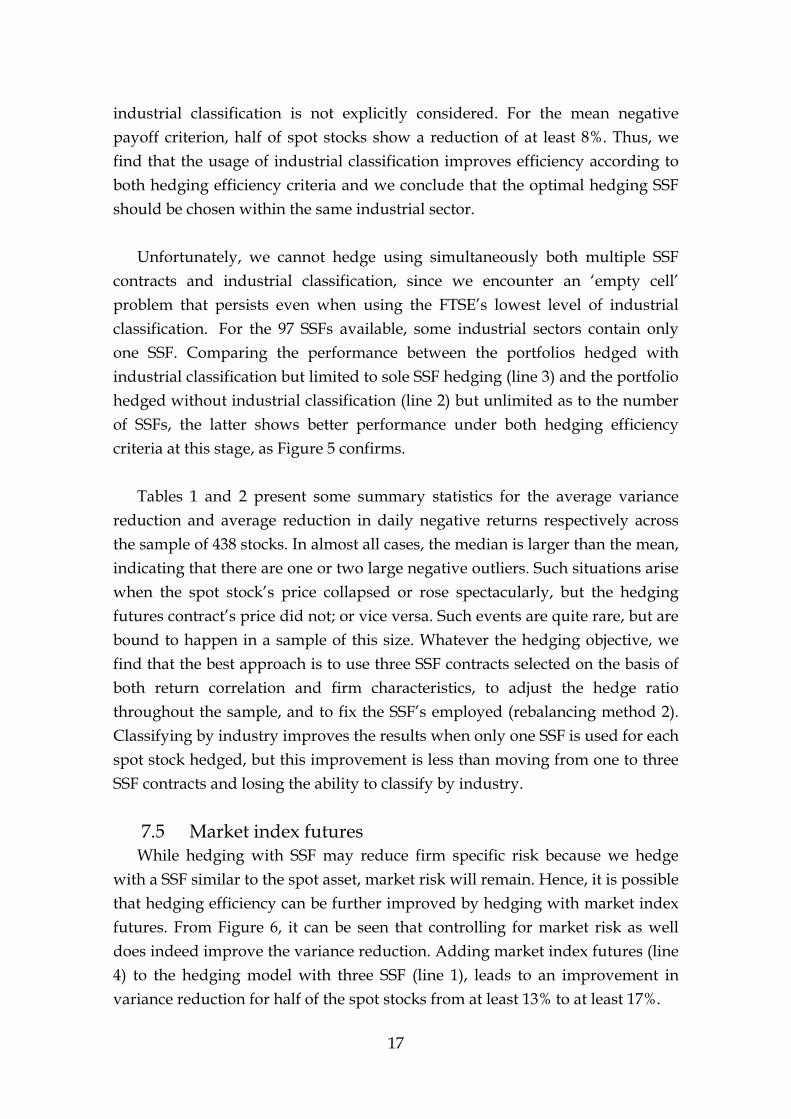
7.3 Multiple SSF contracts If there are benefits from diversification, hedging with multiple SSF

contracts may improve hedging efficiency. In Figure 4, the effect of hedging with multiple SSF contracts (lines 2 and 3) on the variance reduction is compared with that of hedging with only one SSF for each stock (line 1). For hedging with three SSF contracts (line 3), half of the spot stocks show at least a 13% variance reduction and 338 stocks (77%) show a better performance than that of hedging with a single SSF. Similarly, the mean negative payoff is reduced in absolute value as we employ more SSF contracts.

Until this point, we have chosen the optimal SSF contracts without consideration of their industrial sectors – that is, SSF contracts could be matched with spot stocks in totally different industrial sectors. For example, spot stocks in the technology sector could be matched with SSF contracts in the agriculture sector. Therefore, in the following section we examine whether matching SSF contracts within the same industrial sectors as the spot stocks can improve hedging efficiency.

7.4 Industry classification

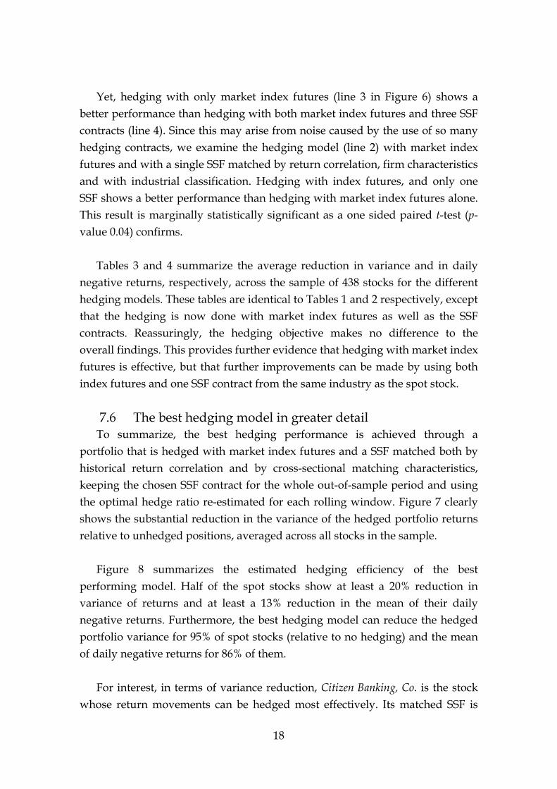
As seen in Figure 5, employing industry classification as an additional matching criterion (line 3) improves hedging efficiency and helps reduces variance, relative to when industry is ignored (line 1). Half of spot stocks now show a variance reduction of at least 9%. Now, 210 spot stocks (48%) show a strictly greater reduction in the variance of the hedged portfolio returns compared with when industrial classification is not explicitly considered. Of the remaining 228 stocks, 90 spot stocks (21%) exhibit the same variance reduction and 138 spot stocks (31%) have less variance reduction than when

17

industrial classification is not explicitly considered. For the mean negative payoff criterion, half of spot stocks show a reduction of at least 8%. Thus, we find that the usage of industrial classification improves efficiency according to both hedging efficiency criteria and we conclude that the optimal hedging SSF should be chosen within the same industrial sector.

Unfortunately, we cannot hedge using simultaneously both multiple SSF

contracts and industrial classification, since we encounter an ‘empty cell’ problem that persists even when using the FTSE’s lowest level of industrial classification. For the 97 SSFs available, some industrial sectors contain only one SSF. Comparing the performance between the portfolios hedged with industrial classification but limited to sole SSF hedging (line 3) and the portfolio hedged without industrial classification (line 2) but unlimited as to the number of SSFs, the latter shows better performance under both hedging efficiency criteria at this stage, as Figure 5 confirms.

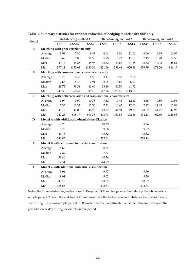
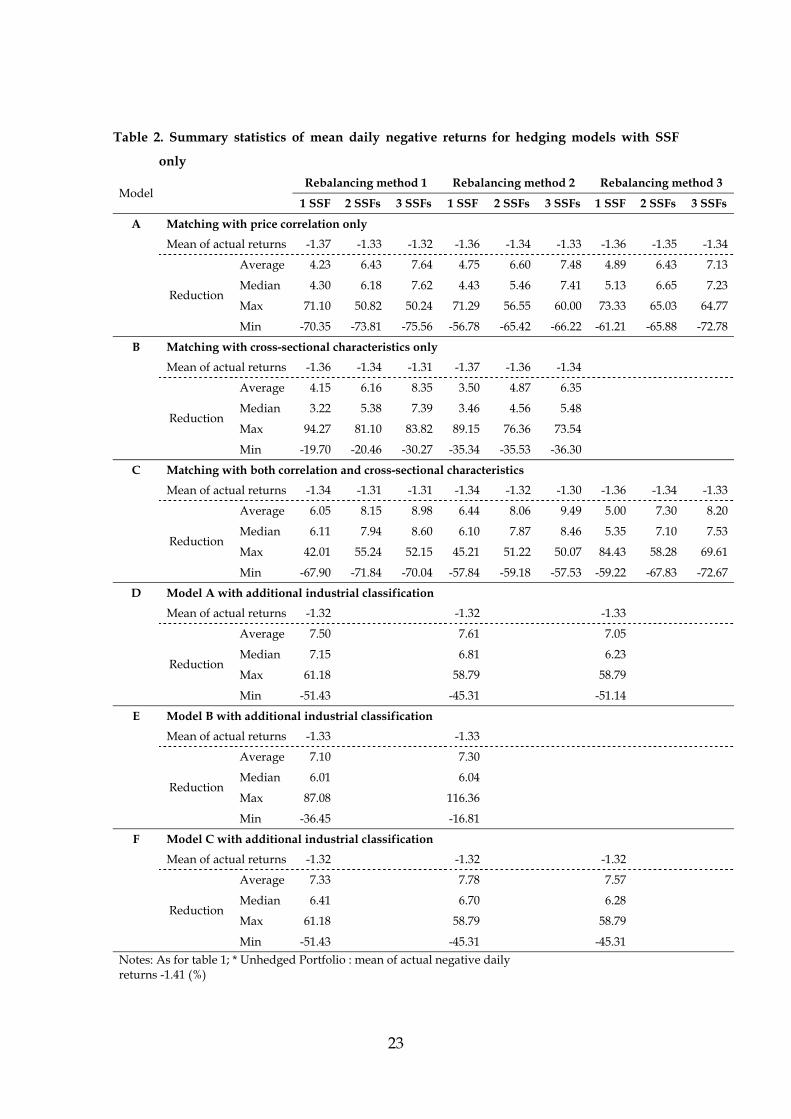
Tables 1 and 2 present some summary statistics for the average variance

reduction and average reduction in daily negative returns respectively across the sample of 438 stocks. In almost all cases, the median is larger than the mean, indicating that there are one or two large negative outliers. Such situations arise when the spot stock’s price collapsed or rose spectacularly, but the hedging futures contract’s price did not; or vice versa. Such events are quite rare, but are bound to happen in a sample of this size. Whatever the hedging objective, we find that the best approach is to use three SSF contracts selected on the basis of both return correlation and firm characteristics, to adjust the hedge ratio throughout the sample, and to fix the SSF’s employed (rebalancing method 2). Classifying by industry improves the results when only one SSF is used for each spot stock hedged, but this improvement is less than moving from one to three SSF contracts and losing the ability to classify by industry.

7.5 Market index futures While hedging with SSF may reduce firm specific risk because we hedge

with a SSF similar to the spot asset, market risk will remain. Hence, it is possible that hedging efficiency can be further improved by hedging with market index futures. From Figure 6, it can be seen that controlling for market risk as well does indeed improve the variance reduction. Adding market index futures (line 4) to the hedging model with three SSF (line 1), leads to an improvement in variance reduction for half of the spot stocks from at least 13% to at least 17%.

18

Yet, hedging with only market index futures (line 3 in Figure 6) shows a

better performance than hedging with both market index futures and three SSF contracts (line 4). Since this may arise from noise caused by the use of so many hedging contracts, we examine the hedging model (line 2) with market index futures and with a single SSF matched by return correlation, firm characteristics and with industrial classification. Hedging with index futures, and only one SSF shows a better performance than hedging with market index futures alone. This result is marginally statistically significant as a one sided paired t-test (p-value 0.04) confirms.

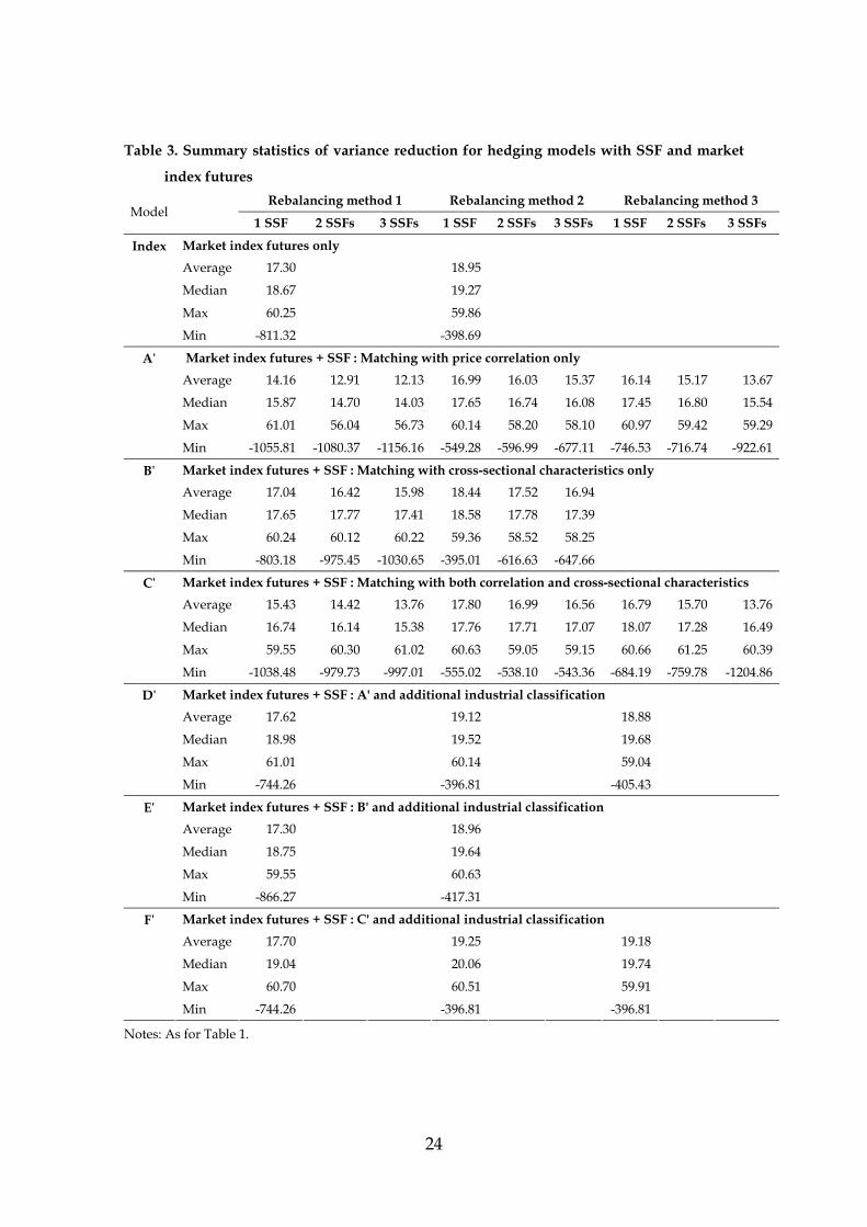
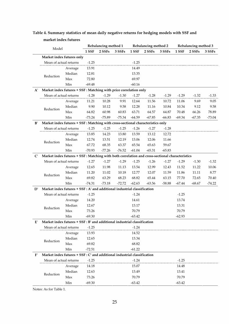
Tables 3 and 4 summarize the average reduction in variance and in daily negative returns, respectively, across the sample of 438 stocks for the different hedging models. These tables are identical to Tables 1 and 2 respectively, except that the hedging is now done with market index futures as well as the SSF contracts. Reassuringly, the hedging objective makes no difference to the overall findings. This provides further evidence that hedging with market index futures is effective, but that further improvements can be made by using both index futures and one SSF contract from the same industry as the spot stock.

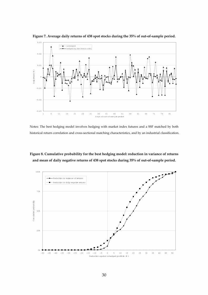
7.6 The best hedging model in greater detail To summarize, the best hedging performance is achieved through a

portfolio that is hedged with market index futures and a SSF matched both by historical return correlation and by cross-sectional matching characteristics, keeping the chosen SSF contract for the whole out-of-sample period and using the optimal hedge ratio re-estimated for each rolling window. Figure 7 clearly shows the substantial reduction in the variance of the hedged portfolio returns relative to unhedged positions, averaged across all stocks in the sample.

Figure 8 summarizes the estimated hedging efficiency of the best

performing model. Half of the spot stocks show at least a 20% reduction in variance of returns and at least a 13% reduction in the mean of their daily negative returns. Furthermore, the best hedging model can reduce the hedged portfolio variance for 95% of spot stocks (relative to no hedging) and the mean of daily negative returns for 86% of them.

For interest, in terms of variance reduction, Citizen Banking, Co. is the stock

whose return movements can be hedged most effectively. Its matched SSF is

19

American Express, Co., which is in the same ‘Financials’ sector. Regarding the mean of negative payoffs, CMGI, Inc. is the stock that can be hedged most effectively. The matched SSF is Hewlett-Packard, Co., which is in the same ‘Information Technology’ sector. During our 85 days out-of-sample period, the mean of daily negative returns reduces by 1.18% on average. Thus, if we assume that the investor had a $10 million position in this stock, over one year the average daily negative payoff would be reduced by $345,828 using the methods described in this paper.

8 Conclusions Investors holding positions in individual stocks may wish to hedge using

futures contracts, but it would be necessary for them to cross hedge (or to hedge with a stock index) in the likely situation that there exists no futures contract on the spot stock(s) that they hold. But the appropriate method for selecting the optimal futures contract is not obvious. Thus, this study examines the use of sample matching techniques together with fundamental firm characteristics for cross hedging with single stock futures. Since individual stocks have very different characteristics from one another, the efficiency of cross-hedging using futures whose underlying asset differs from the spot stock may have been expected to be low. However, we show that an effective hedge can be constructed by matching stocks with SSFs based on their multivariate cross-sectional characteristics and that this hedged portfolio has higher efficiency than a hedged portfolio based on historical return correlations alone.

We show that hedging efficiency can be further improved by using industrial classification to control for industry-specific effects or by using additional SSF contracts to obtain additional diversification. Overall, industrial classification is more important than the use of multiple SSF for hedging efficiency. In addition, eliminating market risk is at least as important as eliminating firm specific risk. Thus, hedging with market index futures as well improves hedging effectiveness compared to hedging with only SSF contracts.

An obvious objective for further study is the use of a longer sample period for estimating the hedge ratios and for determining hedging effectiveness. Our sample period is necessarily limited by the length of time that SSF contracts have been trading. It may also be of interest to examine alternative matching characteristics, such as market-to-book or some measure of recent momentum.

20

References

Anderson, R.W., J. Danthine, 1980. Hedging and Joint Production: Theory and Illustrations. Journal of Finance 35 (2), 487 – 498. Anderson, R.W., J. Danthine, 1981. Cross Hedging. Journal of Political Economy 89 (6), 1182 – 1196. Ang, J.S., Y. Cheng, 2004a. Single Stock Futures: Selection for Listing and Trading Volume. Working Paper, Florida State University. Ang, J.S., Y. Cheng, 2004b. Financial Innovations and Market Efficiency: The Case of Single Stock Futures. Working Paper, Florida State University. Baillie, R.T., R.J. Myers, 1991. Bivariate GARCH Estimation of the Optimal Commodity Futures Hedge. Journal of Applied Econometrics 6 (2), 109 – 124. Brooks, C., J. Chong, 2001. The Cross-Currency Hedging Performance of Implied versus Statistical Forecasting Models. Journal of Futures Markets 21 (11), 1043 – 1069. Brooks, C., O.T. Henry, and G. Persand, 2002. The Effect of Asymmetries on Optimal Hedge Ratios Journal of Business 75(2), 333-352. Cecchetti, S.G., R.E. Cumby, S. Figlewski, 1988. Estimation of the Optimal Futures Hedge. Review of Economics and Statistics 70 (4), 623 – 630. Davies, R.J., S.S. Kim, 2004. Using Matched Samples to Test for Differences in Trade Execution Costs. Working Paper, Babson College. DeMaskey, A.L., 1997. Single and Multiple Portfolio Cross-Hedging with Currency Futures. Multinational Finance Journal 1 (1), 23 – 46. Dutt, H.R., I.L. Wein, 2003. On the Adequacy of Single Stock Futures Margining Requirements. Journal of Futures Markets 23 (10), 989 – 1002. Ederington, L.H., 1979. The Hedging Performance of the New Futures Markets. Journal of Finance 34 (1), 157 – 170.

21

Foster, F.D., C.H. Whiteman, 2002. Bayesian Cross Hedging: An Example from the Soybean Market. Australian Journal of Management 27 (2), 95 – 122. Franken J.R.V., J.L. Parcell, 2003. Cash Ethanol Cross-Hedging Opportunities. Journal of Agricultural and Applied Economics 35 (3), 509 – 516. Hull, J., 2002. Options, Futures, and Other Derivatives (Fifth edition). Prentice Hall. Hung, M.W., C.F. Lee, L.C. So, 2003. Impact of foreign-listed single stock futures on the domestic underlying stock markets. Applied Economics Letters 10(9), 567 – 574. Kroner, F.K., J. Sultan, 1993. Time-varying Distribution and Dynamic Hedging with Foreign Currency Futures. Journal of Financial and Quantitative Analysis 28 (4) 535 – 551. Lascelles, D., 2002. Single Stock Futures, the Ultimate Derivative. CSFI Publications No. 52. Lien, D., 2001a. A Note on Loss Aversion and Futures Hedging. Journal of Futures Markets 21 (7), 681 – 692. Lien, D., 2001b. Futures Hedging under Disappointment Aversion. Journal of Futures Markets 21 (11), 1029 – 1042. Lien, D., Y.K. Tse, 2002. Some Recent Developments in Futures Hedging. Journal of Economic Surveys 16 (3), 357 – 396. McKenzie, M.D., T.J. Brailsford, R.W. Faff, 2001. New Insight into the Impact of the Introduction of Futures Trading on Stock Price Volatility. Journal of Futures Markets 21 (3), 237 – 255. Partnoy, F., 2001. Some Policy Implications of Single-Stock Futures. Working Paper, University of San Diego. Poomimars, P., J. Cadle, M. Thebald, 2003. Futures Hedging Using Dynamic Models of the Variance/Covariance Structure. Journal of Futures Markets 23 (3), 241 – 260.

22

Table 1. Summary statistics for variance reduction of hedging models with SSF only

Rebalancing method 1 Rebalancing method 2 Rebalancing method 3 Model

1 SSF 2 SSFs 3 SSFs 1 SSF 2 SSFs 3 SSFs 1 SSF 2 SSFs 3 SSFs A Matching with price correlation only Average 3.94 7.30 9.47 6.04 9.30 11.10 6.56 9.99 10.95 Median 5.69 9.80 11.50 5.98 9.73 11.65 7.15 10.78 12.58 Max 43.13 45.25 45.98 43.82 46.68 47.88 43.82 47.32 48.84 Min -877.11 -1135.64 -1130.36 -451.56 -588.64 -650.68 -659.79 -671.26 -866.19

B Matching with cross-sectional characteristics only Average 3.78 6.33 8.52 3.11 5.58 7.64 Median 2.68 5.37 7.94 2.05 4.60 6.91 Max 28.72 38.34 41.60 28.40 40.50 41.72 Min -40.30 -50.47 -95.10 -47.96 -79.16 -113.65

C Matching with both correlation and cross-sectional characteristics Average 6.07 9.00 10.78 7.32 10.43 12.37 6.56 9.86 10.56 Median 7.33 10.32 12.56 7.21 10.62 12.60 7.42 11.63 12.99 Max 43.13 41.06 48.25 43.82 41.94 49.22 43.82 44.47 47.93 Min -727.23 -818.17 -893.73 -448.73 -469.65 -492.56 -574.13 -702.60 -1046.68

D Model A with additional industrial classification Average 9.78 10.39 9.76 Median 9.78 9.68 9.22 Max 43.13 43.82 43.82 Min -388.85

-232.64

-259.14

E Model B with additional industrial classification Average 8.66 8.85 Median 7.29 7.73 Max 38.40 40.26 Min -77.31

-44.79

F Model C with additional industrial classification Average 9.04 9.77 9.79 Median 9.01 9.02 9.30 Max 43.13 43.82 43.82 Min -388.85

-232.64

-232.64

Notes: the three rebalancing methods are: 1. Keep both SSF and hedge ratio fixed during the whole out-of-

sample period. 2. Keep the matched SSF, but re-estimate the hedge ratio and rebalance the portfolio every

day during the out-of-sample period. 3. Re-match the SSF, re-estimate the hedge ratio and rebalance the

portfolio every day during the out-of-sample period.

23

Table 2. Summary statistics of mean daily negative returns for hedging models with SSF

only Rebalancing method 1 Rebalancing method 2 Rebalancing method 3

Model 1 SSF 2 SSFs 3 SSFs 1 SSF 2 SSFs 3 SSFs 1 SSF 2 SSFs 3 SSFs

A Matching with price correlation only Mean of actual returns -1.37 -1.33 -1.32 -1.36 -1.34 -1.33 -1.36 -1.35 -1.34

Average 4.23 6.43 7.64 4.75 6.60 7.48 4.89 6.43 7.13

Median 4.30 6.18 7.62 4.43 5.46 7.41 5.13 6.65 7.23

Max 71.10 50.82 50.24 71.29 56.55 60.00 73.33 65.03 64.77

Reduction

Min -70.35 -73.81 -75.56 -56.78 -65.42 -66.22 -61.21 -65.88 -72.78

B Matching with cross-sectional characteristics only Mean of actual returns -1.36 -1.34 -1.31 -1.37 -1.36 -1.34

Average 4.15 6.16 8.35 3.50 4.87 6.35

Median 3.22 5.38 7.39 3.46 4.56 5.48

Max 94.27 81.10 83.82 89.15 76.36 73.54

Reduction

Min -19.70 -20.46 -30.27 -35.34 -35.53 -36.30

C Matching with both correlation and cross-sectional characteristics Mean of actual returns -1.34 -1.31 -1.31 -1.34 -1.32 -1.30 -1.36 -1.34 -1.33

Average 6.05 8.15 8.98 6.44 8.06 9.49 5.00 7.30 8.20

Median 6.11 7.94 8.60 6.10 7.87 8.46 5.35 7.10 7.53

Max 42.01 55.24 52.15 45.21 51.22 50.07 84.43 58.28 69.61

Reduction

Min -67.90 -71.84 -70.04 -57.84 -59.18 -57.53 -59.22 -67.83 -72.67

D Model A with additional industrial classification Mean of actual returns -1.32 -1.32 -1.33

Average 7.50 7.61 7.05

Median 7.15 6.81 6.23

Max 61.18 58.79 58.79

Reduction

Min -51.43 -45.31 -51.14

E Model B with additional industrial classification Mean of actual returns -1.33 -1.33

Average 7.10 7.30

Median 6.01 6.04

Max 87.08 116.36

Reduction

Min -36.45 -16.81

F Model C with additional industrial classification Mean of actual returns -1.32 -1.32 -1.32

Average 7.33 7.78 7.57

Median 6.41 6.70 6.28

Max 61.18 58.79 58.79

Reduction

Min -51.43 -45.31 -45.31 Notes: As for table 1; * Unhedged Portfolio : mean of actual negative daily returns -1.41 (%)

24

Table 3. Summary statistics of variance reduction for hedging models with SSF and market

index futures Rebalancing method 1 Rebalancing method 2 Rebalancing method 3

Model 1 SSF 2 SSFs 3 SSFs 1 SSF 2 SSFs 3 SSFs 1 SSF 2 SSFs 3 SSFs

Index  Market index futures only Average 17.30 18.95

Median 18.67 19.27

Max 60.25 59.86

Min -811.32 -398.69

Aʹ  Market index futures + SSF : Matching with price correlation only Average 14.16 12.91 12.13 16.99 16.03 15.37 16.14 15.17 13.67

Median 15.87 14.70 14.03 17.65 16.74 16.08 17.45 16.80 15.54

Max 61.01 56.04 56.73 60.14 58.20 58.10 60.97 59.42 59.29

Min -1055.81 -1080.37 -1156.16 -549.28 -596.99 -677.11 -746.53 -716.74 -922.61

Bʹ  Market index futures + SSF : Matching with cross-sectional characteristics only Average 17.04 16.42 15.98 18.44 17.52 16.94

Median 17.65 17.77 17.41 18.58 17.78 17.39

Max 60.24 60.12 60.22 59.36 58.52 58.25

Min -803.18 -975.45 -1030.65 -395.01 -616.63 -647.66

Cʹ  Market index futures + SSF : Matching with both correlation and cross-sectional characteristics Average 15.43 14.42 13.76 17.80 16.99 16.56 16.79 15.70 13.76

Median 16.74 16.14 15.38 17.76 17.71 17.07 18.07 17.28 16.49

Max 59.55 60.30 61.02 60.63 59.05 59.15 60.66 61.25 60.39

Min -1038.48 -979.73 -997.01 -555.02 -538.10 -543.36 -684.19 -759.78 -1204.86

Dʹ  Market index futures + SSF : A' and additional industrial classification Average 17.62 19.12 18.88

Median 18.98 19.52 19.68

Max 61.01 60.14 59.04

Min -744.26 -396.81 -405.43

Eʹ  Market index futures + SSF : B' and additional industrial classification Average 17.30 18.96

Median 18.75 19.64

Max 59.55 60.63

Min -866.27 -417.31

Fʹ  Market index futures + SSF : C' and additional industrial classification Average 17.70 19.25 19.18

Median 19.04 20.06 19.74

Max 60.70 60.51 59.91

Min -744.26 -396.81 -396.81

Notes: As for Table 1.

25

Table 4. Summary statistics of mean daily negative returns for hedging models with SSF and

market index futures Rebalancing method 1 Rebalancing method 2 Rebalancing method 3

Model 1 SSF 2 SSFs 3 SSFs 1 SSF 2 SSFs 3 SSFs 1 SSF 2 SSFs 3 SSFs

  Market index futures only Mean of actual returns -1.25 -1.25

Average 13.91 14.49 Median 12.81 13.35 Max 72.80 69.97

Reduction

Min -69.48 -60.16 Aʹ  Market index futures + SSF : Matching with price correlation only

Mean of actual returns -1.28 -1.29 -1.30 -1.27 -1.28 -1.29 -1.29 -1.32 -1.33 Average 11.21 10.28 9.91 12.64 11.56 10.72 11.06 9.69 9.05 Median 9.90 10.12 9.58 12.28 11.16 10.84 10.34 9.12 9.58 Max 64.82 60.98 60.83 63.71 64.57 64.87 70.48 66.26 78.89

Reduction

Min -73.24 -75.89 -75.34 -64.59 -67.85 -66.83 -69.34 -67.35 -73.04 Bʹ  Market index futures + SSF : Matching with cross-sectional characteristics only

Mean of actual returns -1.25 -1.25 -1.25 -1.26 -1.27 -1.28 Average 13.85 14.23 13.80 13.59 13.12 12.72 Median 12.74 13.51 12.19 13.06 12.06 11.66 Max 67.72 68.35 63.37 65.54 65.63 59.67

Reduction

Min -70.93 -77.26 -76.52 -61.04 -65.31 -65.83 Cʹ  Market index futures + SSF : Matching with both correlation and cross-sectional characteristics

Mean of actual returns -1.27 -1.27 -1.29 -1.25 -1.26 -1.27 -1.29 -1.30 -1.32 Average 12.65 11.98 11.13 13.54 12.99 12.43 11.52 11.22 10.06 Median 11.20 11.02 10.18 12.77 12.07 11.59 11.86 11.11 8.77 Max 69.82 63.29 68.23 68.82 65.44 63.15 77.70 72.65 70.40

Reduction

Min -74.31 -73.18 -72.72 -62.63 -63.56 -58.88 -67.44 -68.67 -74.22 Dʹ  Market index futures + SSF : A' and additional industrial classification

Mean of actual returns -1.25 -1.24 -1.25 Average 14.20 14.61 13.74 Median 12.67 13.17 13.31 Max 73.26 70.79 70.79

Reduction

Min -69.30 -63.42 -62.93 Eʹ  Market index futures + SSF : B' and additional industrial classification

Mean of actual returns -1.25 -1.24 Average 13.93 14.52 Median 12.65 13.34 Max 69.82 68.82

Reduction

Min -72.51 -61.22 Fʹ  Market index futures + SSF : C' and additional industrial classification

Mean of actual returns -1.25 -1.24 -1.25 Average 14.18 15.07 14.48 Median 12.63 13.49 13.41 Max 73.26 70.79 70.79

Reduction

Min -69.30 -63.42 -63.42

Notes: As for Table 1.

26

Figure 1. Average variance reduction: comparison of rebalancing procedures.

-8

-4

0

4

8

0.15 0.175 0.2 0.225 0.25 0.275 0.3 0.325 0.35 0.375 0.4 0.425 0.45 0.475 0.5

Propotion of out-of sam ple period out of total sam ple period (% )

Average variance Reduction (%)

123

Notes: Average reduction in variance of returns of 438 spot stocks hedged with a SSF against the

unhedged case. Out-of-sample periods are presented on the x-axis as a portion of the total sample period

with a fixed end point and a variable starting point. Key: 1. Keep both SSF and hedge ratio fixed during

the whole out-of-sample period. 2. Keep the matched SSF, but re-estimate the hedge ratio and rebalance

the portfolio every day during the out-of-sample period. 3. Re-match the SSF, re-estimate the hedge ratio

and rebalance the portfolio every day during the out-of-sample period.

27

Figure 2(i) Variance reduction: comparison of matching characteristics.

0%

25%

50%

75%

100%

-50 -45 -40 -35 -30 -25 -20 -15 -10 -5 0 5 10 15 20 25 30 35 40 45 50

Variance Reduction (% )

Cum

ulative Probability

1

2

3

(ii) Reduction in mean of negative daily returns: comparison of matching characteristics.

0%

25%

50%

75%

100%

-50 -45 -40 -35 -30 -25 -20 -15 -10 -5 0 5 10 15 20 25 30 35 40 45 50

Average reduction in daily negative returns (% )

Cum

ulative Probability

1

2

3

Notes: Figure 2(i) shows the cumulative probability distribution of the reduction in variance of returns of

438 spot stocks hedged with a SSF against the unhedged case. Figure 2(ii) shows the cumulative

probability distribution of the reduction in the average negative daily returns of 438 spot stocks hedged

with a SSF against the unhedged case. Key: 1. Match a SSF with only a historical return correlation. 2.

Match a SSF with only cross-sectional matching characteristics. 3. Match a SSF with both a return

correlation and cross-sectional matching characteristics.

28

Figure 3. Average variance reduction: comparison of different out-of-sample results between

hedging models with different matching characteristics.

-4

-2

0

2

4

6

8

15 17.5 20 22.5 25 27.5 30 32.5 35 37.5 40 42.5 45 47.5 50

Portion of out-of-sam ple period out of total sam ple period (% )

Average variance reduction (%)

1

2

3

Notes: Average reduction in variance of returns of 438 spot stocks hedged with SSF against the unhedged

case. Out-of-sample periods are presented on x-axis as a proportion of total sample period with a fixed end

point and a variable starting point. Key: 1. Match a SSF with only a historical return correlation. 2. Match a

SSF with only matching characteristics. 3. Match a SSF with both a return correlation and matching

characteristics.

Figure 4. Average variance reduction: single SSF versus multiple SSF contracts.

0%

25%

50%

75%

100%

-50 -45 -40 -35 -30 -25 -20 -15 -10 -5 0 5 10 15 20 25 30 35 40 45 50

Variance Reduction (% )

Cum

ulative Probability

1

2

3

Notes: Cumulative probability distribution of reduction in variance of returns of 438 spot stocks hedged

with SSF against the unhedged case. Each SSF is matched with both historical correlation and cross-

sectional matching characteristics. Key: 1. Match a sole SSF. 2. Match two SSFs. 3. Match three SSFs.

29

Figure 5. Average variance reduction: with industrial classification versus without it.

0%

25%

50%

75%

100%

-50 -45 -40 -35 -30 -25 -20 -15 -10 -5 0 5 10 15 20 25 30 35 40 45 50

Variance Reduction (% )

Cumulative Probability

1

2

3

Notes: Cumulative probability distribution of reduction in variance of returns of 438 spot stocks hedged

with SSF against the unhedged case. Key: 1. Match a SSF with both a return correlation and cross-sectional

matching characteristics. 2. Match three SSF with both a return correlation and cross-sectional matching

characteristics. 3. Match a SSF with both a return correlation and cross-sectional matching characteristics

and within the same industrial classification.

Figure 6. Average variance reduction: hedging with market index future vs. without it.

0%

25%

50%

75%

100%

-50 -45 -40 -35 -30 -25 -20 -15 -10 -5 0 5 10 15 20 25 30 35 40 45 50

Variance Reduction (% )

Cum

ulative Probability

1

2

3

4

Notes: Average of reduction in variance of returns for 438 spot stocks hedged with SSF against the

unhedged case. Key: 1. Hedge with three SSF matched by both a historical return correlation and cross-

sectional matching characteristics. 2. Hedge with market index futures and a SSF matched by both a

historical return correlation and cross-sectional matching characteristics, and by an additional industrial

classification. 3. Hedge with market index futures only. 4. Hedge with market index futures and three SSF

matched by both a historical return correlation and cross-sectional matching characteristics.

30

Figure 7. Average daily returns of 438 spot stocks during the 35% of out-of-sample period.

-0.03

-0.02

-0.01

0

0.01

0.02

0.03

1 6 11 16 21 26 31 36 41 46 51 56 61 66 71 76 81

Days of out-of sam ple period

Daily returns (%)

unhedged

hedged by the best m odel

Notes: The best hedging model involves hedging with market index futures and a SSF matched by both

historical return correlation and cross-sectional matching characteristics, and by an industrial classification.

Figure 8. Cumulative probability for the best hedging model: reduction in variance of returns

and mean of daily negative returns of 438 spot stocks during 35% of out-of-sample period.

0%

25%

50%

75%

100%

-50 -45 -40 -35 -30 -25 -20 -15 -10 -5 0 5 10 15 20 25 30 35 40 45 50

Reduction against unhedged portfolio (% )

Cum

ulative probability

Reduction in variance of returns

Reduction in daily negative returns