CRLB Calculations for Joint AoA, AoD and … Calculations for Joint AoA, AoD and Multipath Gain...

CRLB Calculations for Joint AoA, AoD and

Multipath Gain Estimation in Millimeter Wave

Wireless Networks

Laxminarayana S Pillutla and Ramesh Annavajjala

Abstract

In this report we present an analysis of the non-random and the Bayesian Cramer-Rao lower bound

(CRLB) for the joint estimation of angle-of-arrival (AoA), angle-of-departure (AoD), and the multipath

amplitudes, for the millimeter-wave (mmWave) wireless networks. Our analysis is applicable to multipath

channels with Gaussian noise and independent path parameters. Numerical results based on uniform

AoA and AoD in [0, π), and Rician fading path amplitudes, reveal that the Bayesian CRLB decreases

monotonically with an increase in the Rice factor. Further, the CRLB obtained by using beamforming

and combining code books generated by quantizing directly the domain of AoA and AoD was found to

be lower than those obtained with other types of beamforming and combining code books.

This technical report provides detailed calculations with respect to the derivation of non-random and random CRLB for the

joint estimation problem of AoA, AoD and multipath gains.

The first author is with the Dhirubhai Ambani Institute of Information and Communication Technology (DA-

IICT), Gandhinagar, Gujarat, India and the second author is with the NorthEastern University, Boston, MA, USA. E-

mail:[email protected], [email protected]

arX

iv:1

704.

0045

3v1

[cs

.IT

] 3

Apr

201

7

1

CRLB Calculations for Joint AoA, AoD and

Multipath Gain Estimation in Millimeter Wave

Wireless Networks

I. INTRODUCTION

Millimeter wave (mmWave) communications are explored to push data rates in wireless networks to

the order of gigabit per second. Directional transmissions would be used in mmWave networks to counter

the increased path loss at mmWave frequencies (6 GHz and beyond) [1]. This requires accurate beam

alignment on either side of the communication link, a task in turn requires accurate estimation of angle-

of-departure (AoD) and angle-of-arrival (AoA) at the transmitter and receiver respectively. In this report

we consider the fundamental performance limits of joint AoD and AoA estimation, in terms of the well

known Cramer-Rao lower bound (CRLB) computation.

The problem of CRLB computation for AoA estimation alone was previously considered in [2].

However AoD estimation and the signal fading effect (that is inherent in any wireless communication

scenario) were not considered in [2]. The work in [2] further analyzes the statistical efficiency of

MUSIC and maximum-likelihood (ML) methods. Other works that consider AoA estimation and CRLB

computation can be found in [3] and [4]. In [5], Bayesian CRLB was derived for efficient beam tracking

in mmWave communications, which deals with estimation/tracking of AoD only. The joint AoA and

AoD estimation problem and the concomitant channel estimation problem for mmWave communications

was considered in several recent works like those in [6] and [7], to name a few. However, these works

do not deal with CRLB computations.

In this report we consider both the non-random and Bayesian CRLB derivations for the joint AoA

and AoD estimation problem. The derived Bayesian CRLB would serve as a ground truth against which

the performance of any unbiased estimator can be compared. The interested readers are referred to the

monograph in [8] for an exhaustive collection of works on Bayesian bounds for parameter estimation. We

consider a system model that uses pilot symbols at the transmitter and receiver to facilitate the estimation

of AoA and AoD at the receiver. Our specific contributions for the system model we assumed are as

follows:

1) We first derive the non-random CRLB, for the observation model that we assumed, which any

unbiased estimator for AoA and AoD should satisfy (cf. Theorem 1 in Section III-B).

2

2) We next derive the Bayesian CRLB assuming (i) the AoA and AoD distribution to be uniform

(although the underlying calculations are equally suitable for other distributions) and (ii) the signal

fading process on various paths between the transmitter and receiver to be of Rician distribution

(which includes Rayleigh fading and AWGN as special cases) (cf. Proposition 1 in Section III-C).

3) Our numerical results obtained based on the derived Bayesian CRLB point to the following

important conclusions: (i) An increase in the Rice factor causes the Bayesian CRLB to decrease and

(ii) beam forming and combining code books generated by directly quantizing the domain of AoA

and AoD (= [0, π)) resulted in a lower CRLB value compared to the cases, in which beam forming

and combining code books are generated by quantizing the range of AoA and AoD (= [−1, 1])

and the one in which orthogonal beam forming and combining code books are used.

Notation

Throughout this report we use boldface capital alphabets to denote matrices and boldface small

alphabets to denote the vectors. A diagonal matrix is denoted as diag(q) such that its diagonal elements

are equal to the elements of q. The symbols ∗, T and † are used to denote complex conjugate, matrix

transpose and matrix conjugate transpose operators respectively. The Kronecker product between two

matrices A and B is denoted as A⊗B. The mathematical expectation operation is denoted as E[.].

II. SYSTEM MODEL DESCRIPTION OF CHANNEL ESTIMATION IN MILLIMETER WAVE WIRELESS

SYSTEMS

A. System and channel model description

Consider a typical mmWave communication system which comprises of a transmitter and receiver

equipped with uniform linear arrays (ULA) with antenna elements nt and nr respectively. The spac-

ing between antenna elements is assumed to be equal to half of the corresponding radiated signal’s

wavelength. Denote φ and ψ as the angle of arrival (AoD) and angle of arrival (AoA) at the ULA of

transmitter and receiver respectively. The corresponding beamsteering vectors are then given by et(φ) =

1√nt

[1, e−jπ cos(φ), · · · , e−jπ(nt−1) cos(φ)

]Tand er(φ) = 1√

nr

[1, e−jπ cos(ψ), · · · , e−jπ(nr−1) cos(ψ)

]Tre-

spectively. Therefore under the L-path scatterer model the channel matrix H is given by

H =

L∑l=1

αler(ψl)et(φl)†, (1)

where αl > 0 (l = 1, · · · , L) denote the random path gains that are assumed to be Ricean distributed with

the normalized probability density function (PDF) [9, Eq. (2.3-61)] and φl and ψl (which denote AoD

and AoA along path l) are assumed to be uniformly distributed between 0 and π. The CRLB calculations

3

in Section III are equally applicable for other statistical distributions of αl, φl and ψl, so long as they are

mutually independent of each other and also independent of the corresponding parameters across other

paths.

B. Pilot based channel estimation

In this subsection we consider a pilot based method for estimation of the channel gain, AoD and AoA

across various paths at the receiver. The values thus estimated can be used for re-construction of channel

matrix at the receiver.

Let pt and pr denote the number of beamforming and beamcombining pilot symbols used to facilitate

estimation of path gain, AoA and AoD, associated with various paths at the receiver. The beamforming

and beamcombining vectors, associated with the directions φp (p = 1, · · · , pt) and ψp (p = 1, · · · , pr),

are given by fp , et(φp) and gp , er(ψp) respectively (Note: et(.) and er(.) are as defined in Section

II-A). The pth beamforming pilot vector fp transmitted, passes through the channel with matrix defined in

Eq. (1) and is combined at the receiver using the qth beamcombining pilot vector gq. The resulting noisy

observation is given by ypq = g†qHfp + g†qz, where z denotes the received complex noise vector that is

assumed to be proper and Gaussian distributed with mean 0 and covariance matrix σ2vInr . If each of the

pt beamforming pilots are repeated pr times, then they can be combined using the pr beamcombining

pilots at the receiver and the resulting ptpr observations can be expressed in matrix form using matrices

F , [f1, f2, · · · , fpt ] and G , [g1,g2, · · · ,gpr ] as

Y = G†HF + Z ,Define y , vec (Y) (2)

y =

L∑l=1

FT ⊗G†︸︷︷︸A

(e∗t (φl)⊗ er(ψl)) + v , (3)

where Z denotes a complex matrix whose entries are assumed to be uncorrelated and proper, each of

zero mean and variance σ2v and v = vec(Z) (which is a proper complex Gaussian random vector of

mean 0 and covariance matrix σ2vIptpr ). The Eq. (3) is obtained by using Eq. (1) and the following

property: vec(UVW) =(WT ⊗U

)vec(V), where U, V and W are matrices of suitable dimensions

[10, Appendix A].

4

III. CRAMER-RAO LOWER BOUND EXPRESSION FOR UNBIASED CHANNEL ESTIMATOR

A. Log-likelihood ratio of the given observation model

For the purpose of analysis in this section we define the following:

θ , [φ1, · · · , φL, ψ1, · · · , ψL, α1, · · · , αL]T

, et(φl) ,1√nt

[0, ejπ cos(φl), · · · , (nt − 1)ej(nt−1)π cos(φl)

]T,

er(ψl) =1√nr

[0, ejπ cos(ψl), · · · , (nr − 1)ej(nr−1)π cos(ψl)

]Tm ,

L∑l=1

A (e∗t (φl)⊗ er(ψl)) ,

and K , A†A.

The model likelihood function p (y|θ) is given by the PDF of a proper complex Gaussian random vector

with mean vector m and covariance matrix σ2vImrmt

, which is equal to 1πprpt (σ2

v)prpt e− 1

σ2v

(y−m)†(y−m)

[9]. Therefore, the log-likelihood function of the model is given by

L(y) = −prpt ln(πσ2v)−

1

σ2v

[(y −m)† (y −m)

]. (4)

B. FIM Computation and the non-random CRLB

Let θ denote the unbiased estimator of θ, then the CRLB on variance of θ is given by Var(θ)≥

tr(J−1

NR

), where JNR denotes the FIM whose (i, j)th entry is given by JNR(i, j) , −E

[∂2L(y)∂θi∂θj

](E w.r.t

the PDF of (y|θ)). The CRLB of any unbiased estimator of θ defined as in Section III-A is given by

the following theorem.

Theorem 1: For the observation model defined in Eq. (3) the non-random CRLB for any unbiased

estimator of θ is given by tr(J−1NR). The entries of matrix JNR are given as follows: (the term corresponding

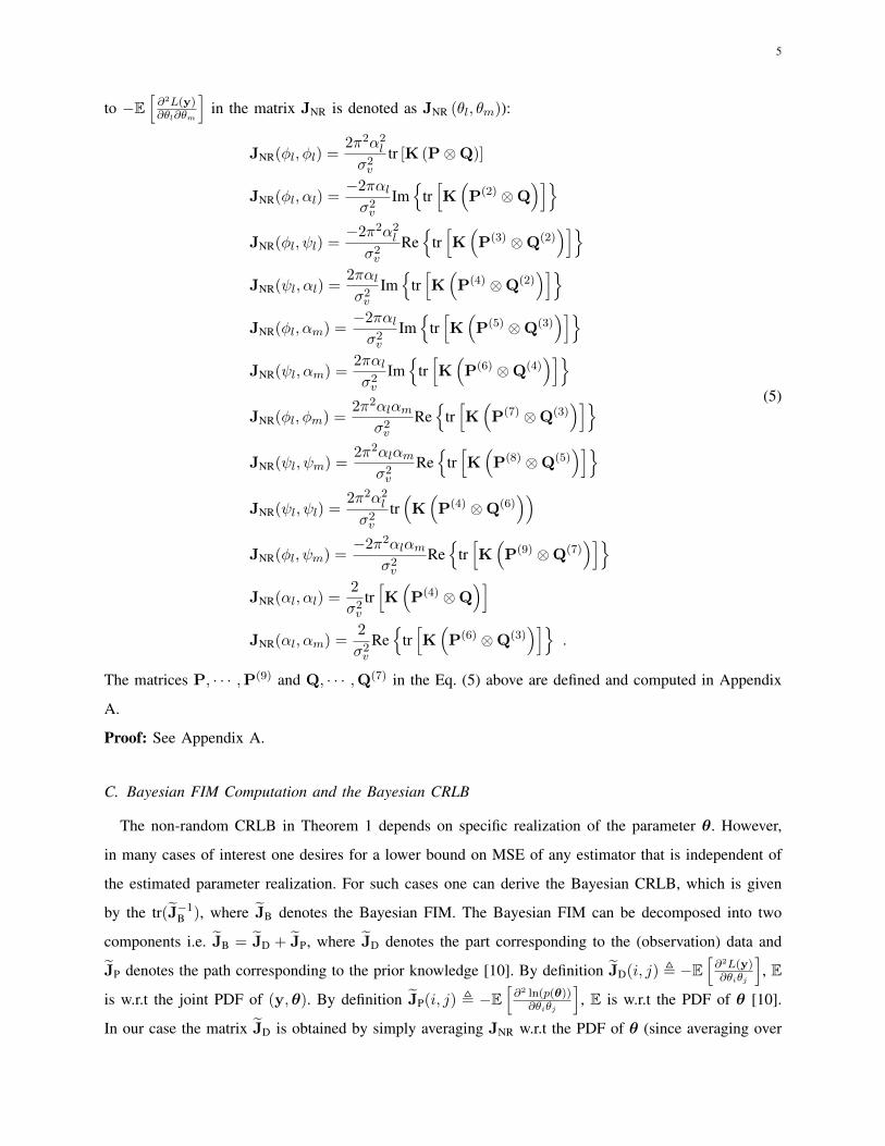
5

to −E[∂2L(y)∂θl∂θm

]in the matrix JNR is denoted as JNR (θl, θm)):

JNR(φl, φl) =2π2α2

l

σ2v

tr [K (P⊗Q)]

JNR(φl, αl) =−2παlσ2v

Im

tr[K(P(2) ⊗Q

)]JNR(φl, ψl) =

−2π2α2l

σ2v

Re

tr[K(P(3) ⊗Q(2)

)]JNR(ψl, αl) =

2παlσ2v

Im

tr[K(P(4) ⊗Q(2)

)]JNR(φl, αm) =

−2παlσ2v

Im

tr[K(P(5) ⊗Q(3)

)]JNR(ψl, αm) =

2παlσ2v

Im

tr[K(P(6) ⊗Q(4)

)]JNR(φl, φm) =

2π2αlαmσ2v

Re

tr[K(P(7) ⊗Q(3)

)]JNR(ψl, ψm) =

2π2αlαmσ2v

Re

tr[K(P(8) ⊗Q(5)

)]JNR(ψl, ψl) =

2π2α2l

σ2v

tr(K(P(4) ⊗Q(6)

))JNR(φl, ψm) =

−2π2αlαmσ2v

Re

tr[K(P(9) ⊗Q(7)

)]JNR(αl, αl) =

2

σ2v

tr[K(P(4) ⊗Q

)]JNR(αl, αm) =

2

σ2v

Re

tr[K(P(6) ⊗Q(3)

)].

(5)

The matrices P, · · · ,P(9) and Q, · · · ,Q(7) in the Eq. (5) above are defined and computed in Appendix

A.

Proof: See Appendix A.

C. Bayesian FIM Computation and the Bayesian CRLB

The non-random CRLB in Theorem 1 depends on specific realization of the parameter θ. However,

in many cases of interest one desires for a lower bound on MSE of any estimator that is independent of

the estimated parameter realization. For such cases one can derive the Bayesian CRLB, which is given

by the tr(J−1B ), where JB denotes the Bayesian FIM. The Bayesian FIM can be decomposed into two

components i.e. JB = JD + JP, where JD denotes the part corresponding to the (observation) data and

JP denotes the path corresponding to the prior knowledge [10]. By definition JD(i, j) , −E[∂2L(y)∂θiθj

], E

is w.r.t the joint PDF of (y,θ). By definition JP(i, j) , −E[∂2 ln(p(θ))∂θiθj

], E is w.r.t the PDF of θ [10].

In our case the matrix JD is obtained by simply averaging JNR w.r.t the PDF of θ (since averaging over

6

the PDF of (y|θ) was already done during the computation of JNR). In averaging the various entries of

JNR w.r.t the PDF of θ, it is worthwhile to note that the gains, AoA and AoD across various paths are

independent of each other. Further for a given path the multipath gain, AoA and AoD are independent

of each other. Similarly JP(i, j) , −E[∂2 ln(p(θ))∂θiθj

], E is w.r.t the PDF of θ which is denoted as p(θ).

For the special case when AoDs and AoAs of all paths (i.e. φlLl=1 and ψlLl=1) are uniformly

distributed between 0 and π, as we assumed in this report, the Bayesian FIM JB and hence CRLB can

be computed as in the following proposition.

Proposition 1: For the special case when φl, ψl (l = 1, · · · , L) are uniformly distributed over [0, π)

the Bayesian CRLB for any unbiased estimator of θ is given by tr(J−1

B

), where the matrix JB = JD +JP.

The entries of JP are all zero except for the following L terms: −E[∂2 ln(p(θ))

∂α2l

](l = 1, · · · , L), whose

expressions can be obtained from Appendix B.

The entries of JD (similar to the entries of JNR) are given below:

JNR(φl, φl) =2π2E[α2

l ]

σ2v

tr[K(P⊗ Q

)]JNR(φl, αl) =

−2πE[αl]

σ2v

Im

tr[K(P(2) ⊗ Q

)]JNR(φl, ψl) =

−2π2E[α2l ]

σ2v

Re

tr[K(P(3) ⊗ Q(2)

)]JNR(ψl, αl) =

2πE[αl]

σ2v

Im

tr[K(P(4) ⊗ Q(2)

)]JNR(φl, αm) =

−2πE[αl]

σ2v

Im

tr[K(P(5) ⊗ Q(3)

)]JNR(ψl, αm) =

2πE[αl]

σ2v

Im

tr[K(P(6) ⊗ Q(4)

)]JNR(φl, φm) =

2π2E[αl]E[αm]

σ2v

Re

tr[K(P(7) ⊗ Q(3)

)]JNR(ψl, ψm) =

2π2E[αl]E[αm]

σ2v

Re

tr[K(P(8) ⊗ Q(5)

)]JNR(ψl, ψl) =

2π2E[α2l ]

σ2v

tr(K(P(4) ⊗ Q(6)

))JNR(φl, ψm) =

−2π2E[αl]E[αm]

σ2v

Re

tr[K(P(9) ⊗ Q(7)

)]JNR(αl, αl) =

2

σ2v

tr[K(P(4) ⊗ Q

)]JNR(αl, αm) =

2

σ2v

Re

tr[K(P(6) ⊗ Q(3)

)].

(6)

The matrices P, · · · , P(9) and Q, · · · , Q(7) in Eq. (6) are defined in Appendix C.

Proof: See Appendix B for the derivation of entries for JP and Appendix C for the derivation of entries

7

for JD.

Following remarks are in order with respect to Proposition 1: (i) For our numerical results evaluation

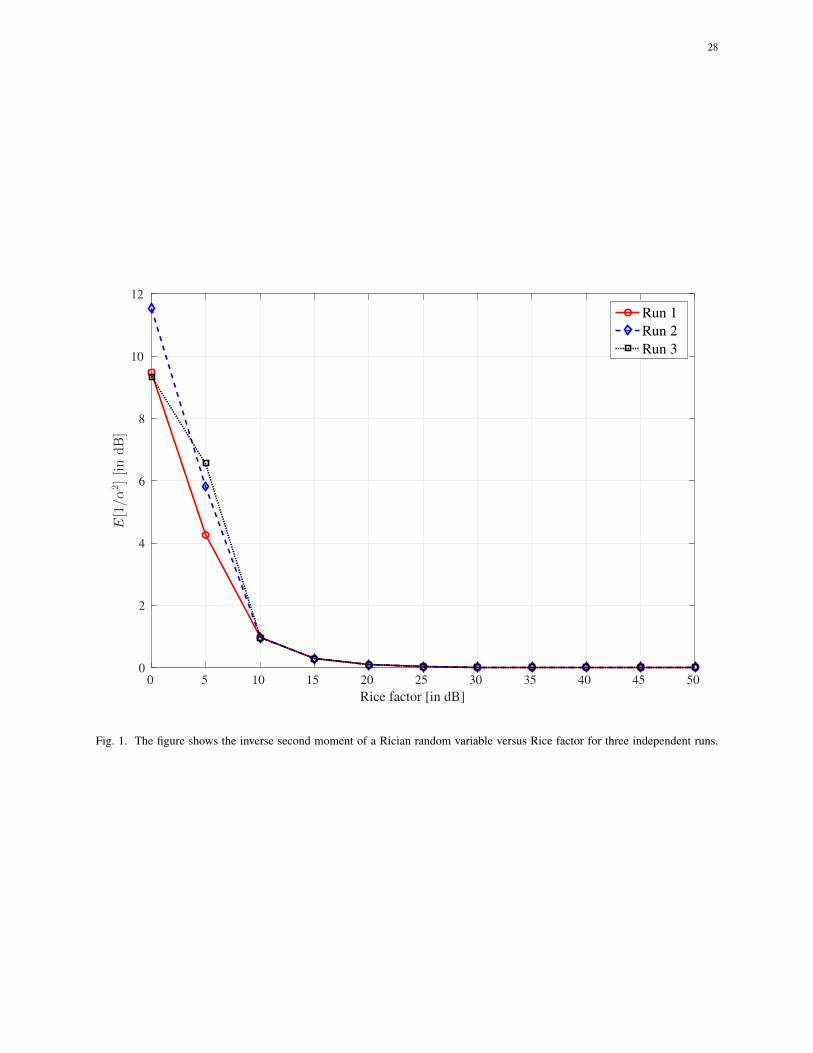
of L non-zero terms of the matrix JP is done using Monte-Carlo (MC) simulations. (ii) For Kl = 0 (i.e.

the Rayleigh fading case) the CRLB becomes undefined, since in this case the non-zero terms of matrix

JP will be equal to E[ 1α2l] =

∫∞0

1α2l

αlσ2le−α

2lσ2l dαl, which diverges to ∞ (since inverting a Rayleigh random

variable would require infinite amount of power). This behavior can also be inferred from Fig. 1, in which

we plot the magnitude of the inverse second moment of a Rician random variable for different values

of Rice factor for three independent runs. For every run the average is computed via MC simulation by

drawing 100000 randomly generated realizations. As can be seen from the Fig. 1 for small values of

Rice factor the magnitude of the inverse second moment is relatively large compared to the case when

the Rice factor is large. Further the value of the inverse second moment for smaller values of Rice factor

are unstable, as can be inferred from the variation in the corresponding value for three different runs.

However, for larger values of Rice factor the value is much more stable and indeed as the Rice factor

gets larger it converges to 1.

The instability or oscillatory behavior observed in Fig. 1 can also be observed in Fig. 2, in which we

plot the Fisher information value (i.e. E[−∂2 ln(p(αl))∂α2

l], E[.] w.r.t p(αl) - Rician PDF, whose expression is

given by [9, Eq. 2.3-61]) of a Rician random variable computed via MC simulations by drawing 100000

randomly generated realizations for three independent runs.

IV. NUMERICAL RESULTS

In this section we plot the derived Bayesian CRLB versus the signal-to-noise ratio (SNR) for different

parameter values of interest.

A. Description of Parameter Values

The SNR at the receiver is equal to ntnr∑Ll=1 Ωl

σ2v

for a normalized transmit power of unity, where

Ωl , E(α2l ). For our numerical results we normalize the sum of average power gains across all paths

to be equal to unity i.e. Ω ,∑L

l=1 Ω2l = 1, therefore in our case SNR = ntnr

σ2v

. Since we assumed

αl (l = 1, · · · , L) to be Ricean distributed therefore let Kl ,µ2l

σ2l

denote the Rice factor of path l. For

an αl of Ricean distribution Ωl = µ2l + σ2

l = σ2l (1 +Kl) [9]. If we assume an exponential power delay

profile for the multi-path channel, then Ωl = Ω1e−(l−1)δ, where δ is the decay parameter associated with

the power delay profile. Since we normalized Ω to unity, therefore we obtain Ω1 = 1∑Ll=1 e

−(l−1)δ . Thus

for a given value of L and δ one can determine Ω1 and thereby set σ2l = Ω1e−(l−1)δ

(1+Kl). For the purpose of

our numerical results we set nt = 16, nr = 16 and δ = 0.5.

8

The beamforming and beamcombining matrices (F and G) are generated in three different methods

as described in the following. The first one referred to as non-uniform method divides the range of

φl and ψl (for every l = 1, · · · , L) respectively i.e. [−1, 1], into pt and pr bins respectively. The

quantized beamforming/beamcombining direction is chosen to be equal to the arccosine of the center

of each bin. This method is tantamount to non-uniform quantization and hence the name. The second

method referred to as uniform divides the range between 0 and π into pt and pr bins. The quantized

beamforming/beamcombining direction is chosen to be equal to the center of each bin. Finally, in the

third method referred to as orthogonal we choose the respective columns of F and G so that they are

orthogonal to each other, thereby implying K = Iptpr .

Note that for Fig. 3 and Fig. 5 we assume the beam forming and combining matrices to be generated

according to the non-uniform method with pt = pr = nt = nr = 16. For Fig. 4 we set the SNR equal to

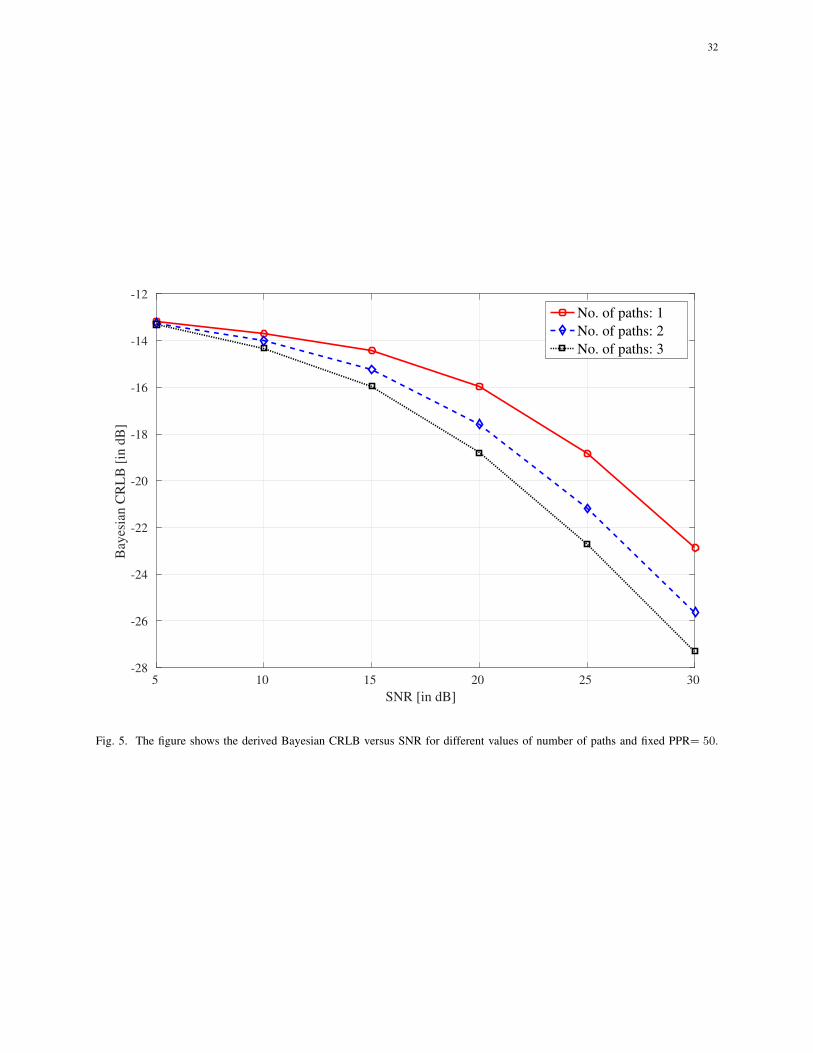
15 dB. For the purpose of our numerical results study in Fig. 5 we introduce the following parameter:

PPR , No. of pilot symbols/No. of estimated parameters.

B. Discussion on numerical results

Fig. 3 contains plots of Bayesian CRLB expression versus SNR for different values of Rice factor.

As can be seen from the plots, in general as SNR increases, CRLB decreases. Also the CRLB for Rice

factor equal to 20 dB is strictly lower than the corresponding CRLB values for Rice factor values equal

to 10 dB and 0 dB respectively. The reason for this trend can be explained as follows: an increase in

Rice factor moves the channel behavior towards that of an AWGN channel, whose CRLB is lower than

that of any fading channel. Further for fixed values of Rice factor and number of pilots, the CRLB for

L = 3 is strictly above that of the case when L = 1. This is because for a fixed pilot budget, the number

of parameters to be estimated increase with an increase in number of paths.

Fig. 2 contains plots of Bayesian CRLB versus the number of pilots for different beamformer types. As

can be seen the CRLB of the uniform beamformer is strictly below that of the non-uniform beamformer

across the entire range of values for number of pilots, although for smaller values of number of pilots the

orthogonal beamformer performs better than the other two. This gives important insights into how the

beam forming and combining code books be designed. Further for all the three types of beamformers,

as expected, the CRLB decreases gradually with an increase in number of pilots.

Finally, Fig. 5 contains plots of Bayesian CRLB versus SNR for a fixed value of PPR= 50. As can

be seen from the plots as the number of paths L increase from 1 to 3 CRLB decreases across all the

SNR values. This is in contrast to what was observed in Fig. 3 this somewhat of a contradictory behavior

can be explained as follows. For the same value of PPR as the number of paths increase, the number

9

of estimated parameters increase, which thereby cause the number of pilots used to also increase, thus

translating into better performance in terms of achieving a lower CRLB.

V. CONCLUSIONS

In this report we derived the random and Bayesian CRLB for the joint estimation problem of AoA,

AoD and multi-path gains. The proposed CRLB shall be useful for comparing the performance of various

practical estimators. Our numerical results based on the derived CRLB point to the following important

observations: (i) an increase in Rice factor in general decreases the CRLB and (ii) the combination of

beam forming and beam combining matrices generated by quantizing the domain of AoA and AoD

(=[0, π)) directly yields a lower CRLB than other methods. As part of our future work we shall consider

extending the joint estimation problem considered in this report by including the elevation angle at both

transmitter and receiver.

10

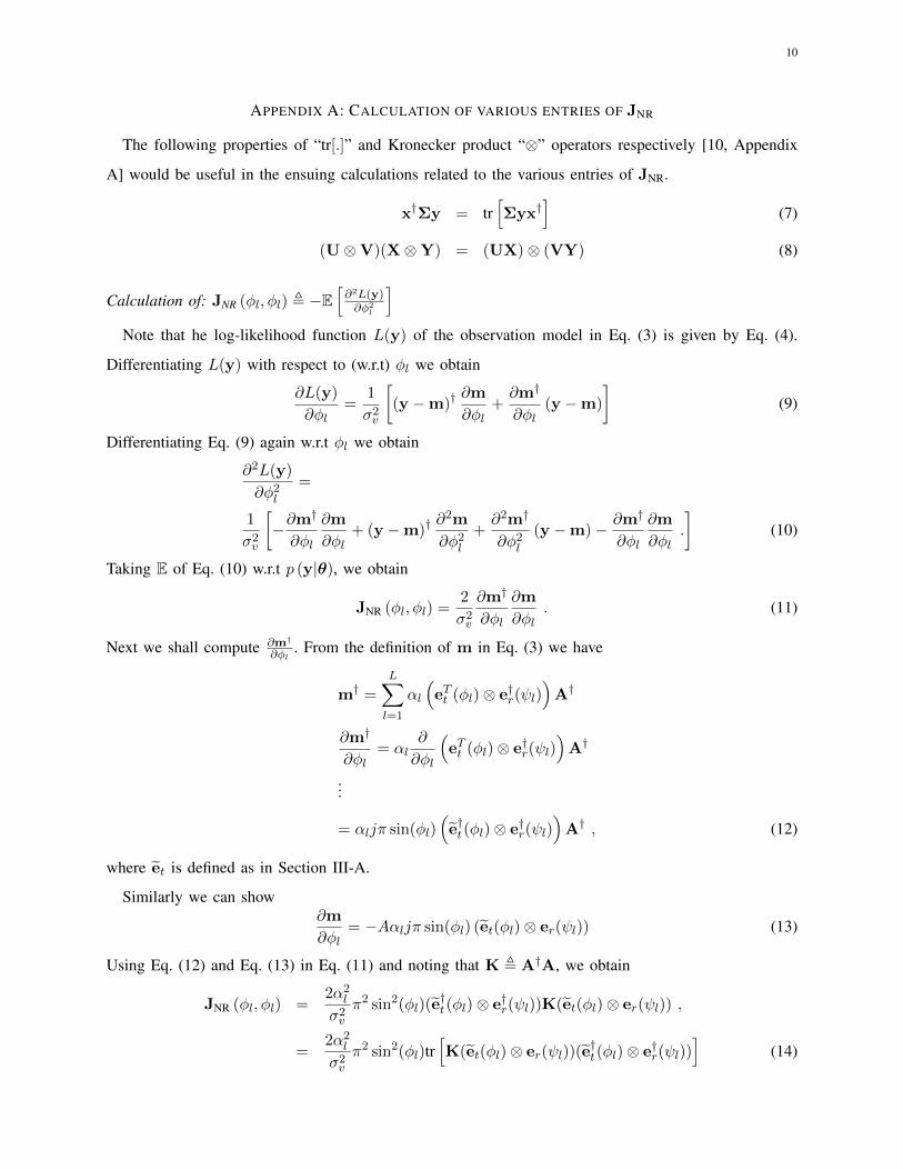
APPENDIX A: CALCULATION OF VARIOUS ENTRIES OF JNR

The following properties of “tr[.]” and Kronecker product “⊗” operators respectively [10, Appendix

A] would be useful in the ensuing calculations related to the various entries of JNR.

x†Σy = tr[Σyx†

](7)

(U⊗V)(X⊗Y) = (UX)⊗ (VY) (8)

Calculation of: JNR (φl, φl) , −E[∂2L(y)∂φ2

l

]Note that he log-likelihood function L(y) of the observation model in Eq. (3) is given by Eq. (4).

Differentiating L(y) with respect to (w.r.t) φl we obtain

∂L(y)

∂φl=

1

σ2v

[(y −m)†

∂m

∂φl+∂m†

∂φl(y −m)

](9)

Differentiating Eq. (9) again w.r.t φl we obtain

∂2L(y)

∂φ2l

=

1

σ2v

[−∂m†

∂φl

∂m

∂φl+ (y −m)†

∂2m

∂φ2l

+∂2m†

∂φ2l

(y −m)− ∂m†

∂φl

∂m

∂φl.

](10)

Taking E of Eq. (10) w.r.t p (y|θ), we obtain

JNR (φl, φl) =2

σ2v

∂m†

∂φl

∂m

∂φl. (11)

Next we shall compute ∂m†

∂φl. From the definition of m in Eq. (3) we have

m† =

L∑l=1

αl

(eTt (φl)⊗ e†r(ψl)

)A†

∂m†

∂φl= αl

∂

∂φl


)A†

...

= αljπ sin(φl)(e†t(φl)⊗ e†r(ψl)

)A† , (12)

where et is defined as in Section III-A.

Similarly we can show∂m

∂φl= −Aαljπ sin(φl) (et(φl)⊗ er(ψl)) (13)

Using Eq. (12) and Eq. (13) in Eq. (11) and noting that K , A†A, we obtain

JNR (φl, φl) =2α2

l

σ2v

π2 sin2(φl)(e†t(φl)⊗ e†r(ψl))K(et(φl)⊗ er(ψl)) ,

=2α2

l

σ2v

π2 sin2(φl)tr[K(et(φl)⊗ er(ψl))(e

†t(φl)⊗ e†r(ψl))

](14)

11

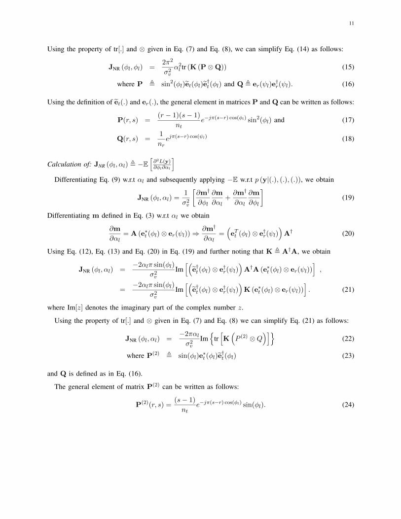
Using the property of tr[.] and ⊗ given in Eq. (7) and Eq. (8), we can simplify Eq. (14) as follows:

JNR (φl, φl) =2π2

σ2v

α2l tr (K (P⊗Q)) (15)

where P , sin2(φl)et(φl)e†t(φl) and Q , er(ψl)e

†r(ψl). (16)

Using the definition of et(.) and er(.), the general element in matrices P and Q can be written as follows:

P(r, s) =(r − 1)(s− 1)

nte−jπ(s−r) cos(φl) sin2(φl) and (17)

Q(r, s) =1

nrejπ(s−r) cos(ψl) (18)

Calculation of: JNR (φl, αl) , −E[∂2L(y)∂φl∂αl

]Differentiating Eq. (9) w.r.t αl and subsequently applying −E w.r.t p (y|(.), (.), (.)), we obtain

JNR (φl, αl) =1

σ2v

[∂m†

∂φl

∂m

∂αl+∂m†

∂αl

∂m

∂φl

](19)

Differentiating m defined in Eq. (3) w.r.t αl we obtain

∂m

∂αl= A (e∗t (φl)⊗ er(ψl))⇒

∂m†

∂αl=(eTt (φl)⊗ e†r(ψl)

)A† (20)

Using Eq. (12), Eq. (13) and Eq. (20) in Eq. (19) and further noting that K , A†A, we obtain

JNR (φl, αl) =−2αlπ sin(φl)

σ2v

Im[(

e†t(φl)⊗ e†r(ψl))

A†A (e∗t (φl)⊗ er(ψl))],

=−2αlπ sin(φl)

σ2v

Im[(


K (e∗t (φl)⊗ er(ψl))]. (21)

where Im[z] denotes the imaginary part of the complex number z.

Using the property of tr[.] and ⊗ given in Eq. (7) and Eq. (8) we can simplify Eq. (21) as follows:

JNR (φl, αl) =−2παlσ2v

Im

tr[K(P (2) ⊗Q

)](22)

where P(2) , sin(φl)e∗t (φl)e

†t(φl) (23)

and Q is defined as in Eq. (16).

The general element of matrix P(2) can be written as follows:

P(2)(r, s) =(s− 1)

nte−jπ(s−r) cos(φl) sin(φl). (24)

12

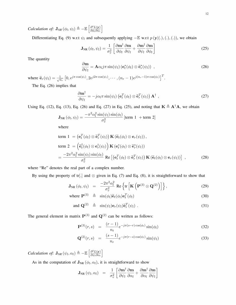
Calculation of: JNR (φl, ψl) , −E[∂2L(y)∂φl∂ψl

]Differentiating Eq. (9) w.r.t ψl and subsequently applying −E w.r.t p (y|(.), (.), (.)), we obtain

JNR (φl, ψl) =1

σ2v

[∂m†

∂φl

∂m

∂ψl+∂m†

∂ψl

∂m

∂φl

](25)

The quantity∂m

∂ψl= Aαljπ sin(ψl) (e∗t (φl)⊗ e∗r(ψl)) , (26)

where er(ψl) = 1√nr

[0, ejπ cos(ψl), 2ej2π cos(ψl), · · · , (nr − 1)ej(nr−1)π cos(ψl)

]T.

The Eq. (26) implies that

∂m†

∂ψl= −jαlπ sin(ψl)

(eTt (φl)⊗ eTr (ψl)

)A† , (27)

Using Eq. (12), Eq. (13), Eq. (26) and Eq. (27) in Eq. (25), and noting that K , A†A, we obtain

JNR (φl, ψl) =−π2α2

l sin(ψl) sin(φl)

σ2v

[term 1 + term 2]

where

term 1 =(eTt (φl)⊗ eTr (ψl)

)K (et(φl)⊗ er(ψl)) ,

term 2 =(e†t(φl)⊗ e†r(ψl)

)K (e∗t (φl)⊗ e∗r(ψl))

=−2π2α2

l sin(ψl) sin(φl)

σ2v

Re[(

eTt (φl)⊗ eTr (ψl))K (et(φl)⊗ er(ψl))

], (28)

where “Re” denotes the real part of a complex number.

By using the property of tr[.] and ⊗ given in Eq. (7) and Eq. (8), it is straightforward to show that

JNR (φl, ψl) =−2π2α2

l

σ2v

Re

tr[K(P(3) ⊗Q(2)

)], (29)

where P(3) , sin(φl)et(φl)eTt (φl) (30)

and Q(2) , sin(ψl)er(ψl)eTr (ψl) . (31)

The general element in matrix P(3) and Q(2) can be written as follows:

P(3)(r, s) =(r − 1)

nte−jπ(s−r) cos(φl) sin(φl) (32)

Q(2)(r, s) =(s− 1)

nre−jπ(r−s) cos(ψl) sin(ψl) (33)

Calculation of: JNR (ψl, αl) , −E[∂2L(y)∂ψl∂αl

]As in the computation of JNR (φl, αl), it is straightforward to show

JNR (ψl, αl) =1

σ2v

[∂m†

∂ψl

∂m

∂αl+∂m†

∂αl

∂m

∂ψl

]

13

Using Eq. (20), Eq. (26) and Eq. (27) in the equation above, which upon further simplification using the

property of tr[.] and ⊗ given in Eq. (7) and Eq. (8) can be simplified to Eq. (35)

JNR (ψl, αl) =2αlπ sin(ψl)

σ2v

Im[(

eTt (φl)⊗ eTr (ψl))K (e∗t (φl)⊗ er(ψl))

](34)

=2αlπ sin(ψl)

σ2v

Im

tr[K (e∗t (φl)⊗ er(ψl))


)]=

2αlπ sin(ψl)

σ2v

Im

tr[K(P(4) ⊗Q(2)

)](35)

where P(4) , e∗t (φl)eTt (φl) , (36)

K , A†A and Q(2) is defined as in Eq. (31).

The general element in matrix P(4) can be written as follows:

P(4)(r, s) =1

ntejπ(r−s) cos(φl). (37)

Calculation of: JNR (φl, αm) , −E[∂2L(y)∂φl∂αm

](l 6= m)

As before it is straightforward to show that

JNR (φl, αm) =1

σ2v

[∂m†

∂φl

∂m

∂αm+∂m†

∂αm

∂m

∂φl

](38)

=−2παl sin(φl)

σ2v

Im[(


K (e∗t (φm)⊗ er(ψm))]

(39)

=−2παl sin(φl)

σ2v

Im

tr[K (e∗t (φm)⊗ er(ψm))

(e†t(φl)⊗ e†r(ψl)

)](40)

=−2παl sin(φl)

σ2v

Im

tr[K(P(5) ⊗Q(3)

)](41)

where P(5) , e∗t (φm) sin(φl)e†t(φl), (42)

Q(3) , er(ψm)e†r(ψl), (43)

and K , A†A. The Eq. (39) follows from Eq. (38) by using Eq. (12), Eq. (13) and Eq. (20). The Eq.

(40) and Eq. (41) follow from Eq. Eq. (39) by using the properties of tr[.] and ⊗ operators respectively

given in Eq. (7) and Eq. (8) respectively.

The general element in matrix P(5) and Q(3) can be written as follows:

P(5)(r, s) =(s− 1)

ntejπ(r−1) cos(φm)e−jπ(s−1) cos(φl) sin(φl) (44)

Q(3)(r, s) =1

nre−jπ(r−1) cos(ψm)ejπ(s−1) cos(ψl) (45)

14

Calculation of: JNR (ψl, αm) , −E[∂2L(y)∂ψl∂αm

](l 6= m)

It is straightforward to show that

JNR (ψl, αm) =1

σ2v

[∂m†

∂ψl

∂m

∂αm+∂m†

∂αm

∂m

∂ψl

](46)

Using Eq. (20), Eq. (26) and Eq. (27) in Eq. (46), and noting that K , A†A, we obtain

JNR (ψl, αm) =2παl sin(ψl)

σ2v

Im[(

eTt (φl)⊗ eTr (ψl))K (e∗t (φm)⊗ er(ψm))

]. (47)

Using the properties of tr[.] and ⊗ operators respectively given in Eq. (7) and Eq. (8) respectively Eq.

(47) can be simplified as follows:

JNR (ψl, αm) =2παl sin(ψl)

σ2v

Im

tr[K (e∗t (φm)⊗ er(ψm))


)]=

2παlσ2v

Im

tr[K(P(6) ⊗Q(4)

)], (48)

where P(6) , e∗t (φm)eTt (φl) =(et(φm)e†t(φl)

)∗(49)

and Q(4) , er(ψm)eTr (ψl) sin(ψl). (50)

The form of P(6) above is similar to the form of Q(3), defined in the calculation of JNR(φl, αm).

Inferring from the generic element of Q(3), we have generic element of the matrix (et(φm)e†t(φl)) to be

the following: 1nte−jπ(r−1) cos(φm)ejπ(s−1) cos(φl). Hence, we have the generic element of P(6) to be the

following:

P(6)(r, s) =1

nt

(e−jπ(r−1) cos(φm)

)∗ (ejπ(s−1) cos(φl)

)∗,

=1

ntejπ(r−1) cos(φm)e−jπ(s−1) cos(φl) . (51)

The generic element of Q(4) can be written as follows:

Q(4)(r, s) =(s− 1)

nre−jπ(r−1) cos(ψm)ejπ(s−1) cos(ψl) sin(ψl) . (52)

Calculation of: JNR (φl, φm) , −E[∂2L(y)∂φl∂φm

](l 6= m)

Differentiating Eq. (10) w.r.t φm and taking −E of the resulting we obtain

JNR (φl, φm) =1

σ2v

[∂m†

∂φl

∂m

∂φm+∂m†

∂φm

∂m

∂φl

](53)

15

The expressions for all the four terms within [.] in the equation above can be gleaned from Eq. (12) and

Eq. (13). Further using K , A†A, we obtain

JNR (φl, φm) =π2 sin(φl) sin(φm)

σ2v

[term 1 + term 2]

where term 1 = αlαm


)K (et(φm)⊗ er(ψm)) ,

and term 2 = αlαm

(e†t(φm)⊗ e†r(ψm)

)K (et(φl)⊗ er(ψl))

=2π2 sin(φl) sin(φm)αlαm

σ2v

Re(


K (et(φm)⊗ er(ψm)). (54)

Using the properties of tr[.] and ⊗ operators respectively given in Eq. (7) and Eq. (8) respectively, we

can simplify Eq. (54) as follows:

JNR (φl, φm) =2π2 sin(φl) sin(φm)αlαm

σ2v

Re

tr[K (et(φm)⊗ er(ψm)) (e†t(φl)⊗ e†r(ψl))

]=

2π2αlαmσ2v

Re

tr[K(P(7) ⊗Q(3)

)], (55)

where P(7) , et(φm)e†t(φl) sin(φm) sin(φl) , (56)

and Q(3) is defined as in Eq. (43).

The generic element of matrix P(7) can be expressed and simplified further to the form given below:

P(7)(r, s) =(r − 1)(s− 1)

ntejπ(r−1) cos(φm) sin(φm)e−jπ(s−1) cos(φl) sin(φl) (57)

Calculation of: JNR (ψl, ψm) , −E[∂2L(y)∂ψl∂ψm

](l 6= m)

As in the calculation of JNR (φl, φm) immediately above, one can show

JNR (ψl, ψm) =1

σ2v

[∂m†

∂ψl

∂m

∂ψm+∂m†

∂ψm

∂m

∂ψl

](58)

The expressions for all the four terms within [.] in the equation above can be gleaned from Eq. (26) and

Eq. (27). Further using K , A†A, we obtain

JNR (ψl, ψm) =π2 sin(ψl) sin(ψm)

σ2v

[term 1 + term 2]

where term 1 = αlαm(eTt (φm)⊗ eTr (ψm)

)K (e∗t (φl)⊗ e∗r(ψl)) ,

and term 2 = αlαm(eTt (φl)⊗ eTr (ψl)

)K (e∗t (φm)⊗ e∗r(ψm))

=2π2 sin(ψl) sin(ψm)αlαm

σ2v

Re(

eTt (φm)⊗ eTr (ψm))K (e∗t (φl)⊗ e∗r(ψl))

. (59)

16

The Eq. (59) can further be simplified using the properties of tr[.] and ⊗ operators respectively given

in Eq. (7) and Eq. (8) respectively as follows:

JNR (ψl, ψm) =2π2 sin(ψl) sin(ψm)αlαm

σ2v

Re

tr[K(e∗t (φl)⊗ e∗r(ψl))(e

Tt (φm)⊗ eTr (ψm))

],

=2π2αlαm

σ2v

Re

tr[K(P(8) ⊗Q(5)

)], (60)

where P(8) , e∗t (φl)eTt (φm) (61)

and Q(5) = e∗r(ψl)eTr (ψm) sin(ψl) sin(ψm) (62)

The generic element of P(8) and Q(5) can be expressed as follows:

P(8)(r, s) =1

ntejπ(r−1) cos(φl)e−jπ(s−1) cos(φm) , (63)

Q(5)(r, s) =(r − 1)(s− 1)

nre−jπ(r−1) cos(ψl) sin(ψl)e

jπ(s−1) cos(ψm) sin(ψm) . (64)

Calculation of: JNR (ψl, ψl) , −E[∂2L(y)∂ψ2

l

]Setting l = m in Eq. (59) we obtain

JNR (ψl, ψl) =2π2 sin2(ψl)α

2l

σ2v


)K (e∗t (φl)⊗ e∗r(ψl)) . (65)

Using the properties of tr[.] and ⊗ operators respectively given in Eq. (7) and Eq. (8) respectively we

can simplify Eq. (65) as follows:

JNR (ψl, ψl) =2π2 sin2(ψl)α

2l

σ2v

[K(e∗t (φl)⊗ e∗r(ψl))e

Tt (φl)⊗ eTr (ψl)

]=

2π2α2l

σ2v

tr[K(P(4) ⊗Q(6)

)], (66)

where Q(6) , e∗r(ψl)eTr (ψl) sin2(ψl) =

(er(ψl)e

†r(ψl) sin2(ψl)

)∗, (67)

and P(4) is defined as in Eq. (36).

The form of Q(6) above is similar to the form of P, defined in the calculation of JNR (φl, φl). Inferring

from the generic element of P, we have generic element of the matrix(er(ψl)e

†r(ψl) sin2(ψl)

)to be

the following: (r−1)(s−1)nr

e−jπ(s−r) cos(ψl) sin2(ψl). Hence, we have the generic element of Q(6) to be the

following:

Q(6)(r, s) =(r − 1)(s− 1)

nr

(e−jπ(s−r) cos(ψl) sin2(ψl)

)∗=

(r − 1)(s− 1)

nrejπ(s−r) cos(ψl) sin2(ψl) (68)

17

Calculation of: JNR (φl, ψm) , −E[∂2L(y)∂φlψm

]Differentiating Eq. (9) w.r.t ψm we obtain

JNR (φl, ψm) =1

σ2v

[∂m†

∂ψm

∂m

∂φl+∂m†

∂φl

∂m

∂ψm

](69)

The expressions for all the four terms within [.] in the equation above can be gleaned from Eq. (12), Eq.

(13), Eq. (26) and Eq. (27) respectively. Further noting that K , A†A, we obtain

JNR (φl, ψm) =−π2 sin(φl) sin(ψm)

σ2v

[term 1 + term 2]

term 1 = αlαm(eTt (φm)⊗ eTr (ψm)


term 2 = αlαm


)K (e∗t (φm)⊗ e∗r(ψm))

=−2π2 sin(φl) sin(ψm)

σ2v

Reαlαm

(eTt (φm)⊗ eTr (ψm)


.(70)


can simplify Eq. (70) as follows

JNR (φl, ψm) =−2π2 sin(φl) sin(ψm)αlαm

σ2v

Re

tr[(K(et(φl)⊗ er(ψl))(e

Tt (φm)⊗ eTr (ψm))

]=−2π2 sin(φl) sin(ψm)αlαm

σ2v

Re

tr[K(P(9) ⊗Q(7)

)], (71)

where P(9) , et(φl)eTt (φm) sin(φl) , (72)

and Q(7) , er(ψl)eTr (ψm) sin(ψm) . (73)

The generic element of P(9) and Q(7) can be expressed as follows:

P(9)(r, s) =(r − 1)

ntejπ(r−1) cos(φl) sin(φl)e

−jπ(s−1) cos(φm) , (74)

Q(7)(r, s) =(s− 1)

nre−jπ(r−1) cos(ψl)ejπ(s−1) cos(ψm) sin(ψm) . (75)

Calculation of: JNR (αl, αl) , −E[∂2L(y)∂α2

l

]Differentiating Eq. (4) w.r.t αl and applying E operator w.r.t the PDF p (y|θ) we obtain

JNR (αl, αl) =2

σ2v

∂m†

∂αl

∂m

∂αl(76)

Using Eq. (20) in Eq. (76) and noting that K , A†A, we obtain

JNR (αl, αl) =2

σ2v


)K (e∗t (φl)⊗ er(ψl)) (77)

18



JNR (αl, αl) =2

σ2v

tr[K(e∗t (φl)⊗ er(ψl))(e

Tt (φl)⊗ e†r(ψl))

]=

2

σ2v

tr[K(P(4) ⊗Q

)], (78)

where Q and P(4) are defined as in Eq. (16) and Eq. (36).

Calculation of: JNR (αl, αm) , −E[∂2L(y)∂αl∂αm

]Differentiating Eq. (4) w.r.t αl and αm successively and applying E operator w.r.t the PDF p (y|θ) we

obtain

JNR (αl, αm) =1

σ2v

[∂m†

∂αl

∂m

∂αm+∂m†

∂αm

∂m

∂αl

](79)

Using Eq. (20) in Eq. (79) and noting that K , A†A, we obtain

JNR (αl, αm) =2

σ2v

Re

(eTt (φl)⊗ e†r(ψl))K(e∗t (φm)⊗ er(ψm)). (80)



JNR (αl, αm) =2

σ2v

Re

tr[K(e∗t (φm)⊗ er(ψm))(eTt (φl)⊗ e†r(ψl))

],

=2

σ2v

Re

tr[K(P(6) ⊗Q(3)

)], (81)

where Q(3) and P(6) are defined as in Eq. (43) and Eq. (49).

APPENDIX B: CALCULATION OF VARIOUS ENTRIES OF JP

As noted in Section III-C the Bayesian FIM JB contains two parts namely: JP and JD. In this section

we shall compute the entries of JP.

We assumed φl and ψl (l = 1, · · · , L) are uniformly distributed over [0, π] and αl (l = 1, · · · , L)

to be of Rician distribution. Further all the parameters are assumed to be independent of each other,

therefore we have

p(θ) =

(1

π

)2L

ΠLl=1pα(αl) , (82)

where pα(α) = 2(K+1)Ω αe−

(K+1)

Ω (α2+ ΩK

K+1)I0

(2α

√K(K+1)

Ω

)denotes a Rician distribution with parame-

ters K (Rice factor) and Ω (second moment) [9].

In general the (i, j)th entry of the matrix JP is given by −E[∂2 ln(p(θ))∂θi∂θj

](E is w.r.t the PDF of θ i.e.

p(θ)). Since p(θ) is independent of φl and ψl, therefore the following terms for any l and m would be

19

zero: JP(φl, ψm) , −E[∂2 ln(p(θ))∂φl∂φm

], JP(φl, αm) , −E

[∂2 ln(p(θ))∂φl∂αm

]and JP(ψl, αm) , −E

[∂2 ln(p(θ))∂ψl∂αm

].

Further for l 6= m, JP(αl, αm) , −E[∂2 ln(p(θ))∂αl∂αm

]will also be equal to 0.

From the above one can conclude that the matrix JP would be all zero except for the following L

terms. These L terms are JP(αl, αl) , −E[∂2 ln(p(θ))

∂α2l

](l = 1, · · · , L). It is a straightforward exercise

to show that

∂2 ln(p(θ))

∂α2l

=−1

α2l

− 2 (Kl + 1)

Ωl+

2Kl (Kl + 1)

Ωl[1 + term 1 + term 2] (83)

where term 1 =

−J2

(−2jαl

√Kl(Kl+1)

Ωl

)I0

(2αl

√Kl(Kl+1)

Ωl

)

and term 2 =

2

(J1

(−2jαl

√Kl(Kl+1)

Ωl

))2

(I0

(2αl

√Kl(Kl+1)

Ωl

))2 .

In the last two equations above Kl denotes the Rice factor of path l and Ωl denotes the second moment

of path l which is defined as in Section IV-A. For each l = 1, · · · , L, JP(αl, αl) can be computed by

taking E of the term given in Eq. (83) w.r.t the PDF of θ i.e. p(θ) (since all the components of θ are

independent of each other this is equivalent to simply taking E w.r.t the PDF of αl i.e. pα(αl)).

APPENDIX C: CALCULATION OF VARIOUS ENTRIES OF JD

In general the (i, j)th entry of the matrix JD is given by −E[∂2L(y)∂θi∂θj

](E is w.r.t the joint PDF of y

and θ i.e. p(y,θ)). Since the (i, j)th entry of JNR is obtained by averaging ∂2L(y)∂θi∂θj

w.r.t the PDF of (y|θ),

therefore (i, j)th entry of JD can be obtained by averaging the corresponding entry of JNR w.r.t the PDF

of θ. Using this fact we shall compute the various entries of JD in the ensuing calculations.

Before we proceed to the actual calculations we shall state a few well known integral expressions and

their closed forms which would be useful for all the calculations in this section.

Consider the following integral

1

π

∫ π

0sin2(θ)ejz cos(θ)dθ

=1

π

∫ π

0

(1− cos(2θ)

2

)ejz cos(θ)dθ

=1

π

∫ π

0

1

2ejz cos(θ)dθ − 1

π

∫ π

0

1

2cos(2θ)ejz cos(θ)dθ

=1

2J0(z)− 1

2

J2(z)

j−2

=1

2[J0(z) + J2(z)] , (84)

20

where the second last equation follows from the following definition of an nth order Bessel function of

first kind: Jn(z) , 1π

∫ π0 ejz cos(θ) cos(nθ)dθ.

Next consider the following integral∫ π

0ejπz cos(θ) sin(θ)dθ =

(2

z

)1/2

J1/2(z) , (85)

where the above equation follows from the the following result from Gradshteyn and Ryhik’s book

on integral tables (pg. 486 Sect. 3.915, Eq. (5)):∫ π

0 ejβ cos(x) sin2ν(x)dx =√π(

2β

)νΓ(ν + 1

2

)Jν(β)(

Re(ν) > −12

).

Calculation of JD(φl, φl) , E [JNR(φl, φl)]

Applying expectation operator w.r.t the joint PDF of φl, ψl and αl i.e. p(θ) defined in Eq. (82), we

can express Eq. (15) as follows:

E [JNR(φl, φl)] =2π2

σ2v

E[α2l ]tr[K(P⊗ Q

)](86)

where P , E[P] and Q , E[Q] . (87)

The general elements of matrices P and Q can be written as below, using the expressions for general

elements of matrices P and Q in Eq. (17) and Eq. (18) respectively:

P(r, s) =(r − 1)(s− 1)

ntE[e−jπ(s−r) cos(φl) sin2(φl)

](88)

Q(r, s) =1

nrE[ejπ(s−r) cos(ψl)

](89)

Since we assumed a uniform distribution over [0, π) for both φl and ψl, therefore Eq. (88) and Eq. (89)

can be simplified to the following:

P(r, s) =(r − 1)(s− 1)

nt

1

π

∫ π

0e−jπ(s−r) cos(φl) sin2(φl)dφl (90)

=(r − 1)(s− 1)

2nt[J0(−π(s− r)) + J2(−π(s− r))] (91)

=1

nr

1

π

∫ π

0ejπ(s−r) cos(ψl)dψl (92)

Q(r, s) =1

nrJ0 (π(s− r)) . (93)

The Eq. (90) follows from Eq. (91) by using Eq. (84) and Eq. (92) follows from Eq. (93) by using the

definition of an nth order Bessel function of first kind.

21

Calculation of JD(φl, αl) , E [JNR(φl, αl)]

JD(φl, αl) =−2πE[αl]

σ2v

Im

tr[K(P(2) ⊗ Q

)](94)

where P(2) , E[P(2)] , (95)

and Q is defined as in Eq. (87).

The general element of matrix P(2) can be written, using the expression for the general element of P

in Eq. (24), as follows:

P(2)(r, s) =(s− 1)

ntE[e−jπ(s−r) cos(φl) sin(φl)

](96)

Since we assumed a uniform distribution over [0, π) for φl, therefore Eq. (96) can be simplified to the

following form:

P(2)(r, s) =(s− 1)

nt

1

π

∫ π

0e−jπ(s−r) cos(φl) sin(φl)dφl (97)

=

2(s−1)πnt

r = s

(s−1)nt

1π

√−2s−rJ1/2 (−π(s− r)) r 6= s

, (98)

where Eq. (98) follows from Eq. (97) by using Eq. (85).

Calculation of JD(φl, ψl) , E [JNR(φl, ψl)]

JD(φl, ψl) =−2π2E[α2

l ]

σ2v

Re

tr[K(P(3) ⊗ Q(2)

)], (99)

where P(3) , E[P(3)

]and Q(2) , E

[Q(2)

](100)

The general element in matrix P(3) and Q(2), using the general element form of matrices P(3) and Q(2)

given by Eq. (32) and Eq. (33) respectively, can be written as follows:

P(3)(r, s) =(r − 1)

ntE[e−jπ(s−r) cos(φl) sin(φl)

](101)

Q(2)(r, s) =(s− 1)

nrE[e−jπ(r−s) cos(ψl) sin(ψl)

](102)

22

Since we assumed a uniform distribution over [0, π) for both φl and ψl, the Eq. (101) and Eq. (102)

can be simplified as follows:

P(3)(r, s) =(r − 1)

nt

1

π

∫ π

0e−jπ(s−r) cos(φl) sin(φl)dφl (103)

=

2(r−1)πnt

r = s

(r−1)nt

1π

√−2s−rJ1/2 (−π(s− r)) r 6= s

(104)

Q(2)(r, s) =(s− 1)

nr

1

π

∫ π

0e−jπ(r−s) cos(ψl) sin(ψl)dψl (105)

=

2(s−1)πnr

r = s

(s−1)nr

1π

√−2r−sJ1/2 (−π(r − s)) r 6= s

(106)

The Eq. (104) follows from Eq. (103) and similarly Eq. (106) follows from Eq. (105), by using Eq. (85).

Calculation of JD(ψl, αl) , E [JNR(ψl, αl)]

JD(ψl, αl) =2πE[αl]

σ2v

Im

tr[K(P(4) ⊗ Q(2)

)], (107)

where P(4) , E[P(4)] , (108)


Using the expression for general element of matrix P(4) in Eq. (37), the general element of matrix

P(4) can be written as follows:

P(4)(r, s) =1

ntE[ejπ(r−s) cos(φl)

](109)

Since we assumed a uniform distribution, over [0, π) for both φl and ψl, therefore can simplify Eq. (109)

to the expression below:

P(4)(r, s) =1

π

∫ π

0ejπ(r−s) cos(φl)dφl =

J0 (π(r − s))nt

, (110)

where the right most term follows from the definition of an nth order Bessel function of first kind.

Calculation of JD(φl, αm) , E [JNR(φl, αm)]

JD(φl, αm) =−2πE[αl]

σ2v

Im

tr[K(P(5) ⊗ Q(3)

)], (111)

where P(5) , E[P(5)

]and Q(3) , E

[Q(3)

](112)

23

Using expressions for general element of matrices P(5) Q(3) given by Eq. (44) and Eq. (45), the general

elements of matrices P(5) and Q(3) can be written as follows:

P(5)(r, s) =(s− 1)

ntE[ejπ(r−1) cos(φm)

]E[e−jπ(s−1) cos(φl) sin(φl)

](113)

Q(3)(r, s) =1

nrE[e−jπ(r−1) cos(ψm)

]E[ejπ(s−1) cos(ψl)

]. (114)

Since we assumed a uniform distribution, over [0, π) for both φl and ψl, therefore we can simplify Eq.

(113) and Eq. (114) to the following expressions:

P(5)(r, s) =(s− 1)

ntJ0 ((r − 1)π)

1

π

∫ π

0e−jπ(s−1) cos(φl) sin(φl)dφl (115)

=(s− 1)

ntJ0 ((r − 1)π)

1

π

√−2

s− 1J1/2(−π(s− 1)) (116)

Q(3)(r, s) =1

nr

1

π

∫ π

0e−jπ(r−1) cos(ψm)dψm

1

π

∫ π

0ejπ(s−1) cos(ψl) (117)

=1

nrJ0 (−(r − 1)π) J0 ((s− 1)π) . (118)

The Eq. (116) follows from Eq. (115) by using Eq. (85), while Eq. (118) follows from Eq. (117) by

using the definition of an nth order Bessel function of first kind.

Calculation of JD(ψl, αm) , E [JNR(ψl, αm)]

JD(ψl, αm) =2πE[αl]

σ2v

Im

tr[K(P(6) ⊗ Q(4)

)], (119)

where P(6) , E[P(6)

]and Q(4) , E

[Q(4)

]. (120)

Using expressions for general element of matrices P(6), Q(4) given by Eq. (51) and Eq. (52), the general


P(6)(r, s) =1

ntE[ejπ(r−1) cos(φm)

]E[e−jπ(s−1) cos(φl)

](121)

Q(4)(r, s) =(s− 1)

nrE[e−jπ(r−1) cos(ψm)

]E[ejπ(s−1) cos(ψl) sin(ψl)

]. (122)

24

Since we assumed φl, φm, ψl and ψm to be uniformly distributed over [0, π), therefore we can simplify

Eq. (121) and Eq. (122) to the following expressions:

P(6)(r, s) =1

nt

1

π

∫ π

0ejπ(r−1) cos(φm)dφm

1

π

∫ π

0e−jπ(s−1) cos(φl)dφl (123)

=1

ntJ0 ((r − 1)π) J0 (−(s− 1)π) (124)

Q(4)(r, s) =

((s− 1)

nr

1

π

∫ π

0e−jπ(r−1) cos(ψm)dψm

)(1

π

∫ π

0ejπ(s−1) cos(ψl) sin(ψl)dψl

)(125)

=

((s− 1)

nrJ0 (−(r − 1)π)

)(1

π

√2

s− 1J1/2 (π(s− 1))

). (126)

The Eq. (124) follows from Eq. (123) by using the definition of an nth order Bessel function of first

kind. The Eq. (126) follows from Eq. (125) by using Eq. (85).

Calculation of JD(φl, φm) , E [JNR(φl, φm)]

JD(φl, φm) =2π2E[αl]E[αm]

σ2v

Re

tr[K(P(7) ⊗ Q(3)

)], (127)

where P(7) , E[P(7)] , (128)


The general element of matrix P(7) can be expressed using the expression for general element of matrix

P(7) given by Eq. (57) and simplified further by noting that φl, φm to be independent and uniformly

distributed over [0, π):

P(7)(r, s) =(r − 1)(s− 1)

ntE[ejπ(r−1) cos(φm) sin(φm)

]E[e−jπ(s−1) cos(φl) sin(φl)

](129)

=(r − 1)(s− 1)

nt

1

π

∫ π

0ejπ(r−1) cos(φm) sin(φm)dφm

1

π

∫ π

0e−jπ(s−1) cos(φl) sin(φl)dφl

=

((r − 1)(s− 1)

nt

1

π

√2

r − 1J1/2(π(r − 1))

)(1

π

√−2

s− 1J1/2(−π(s− 1))

). (130)

The Eq. (130) follow from the equation above it by using Eq. (85).

Calculation of JD(ψl, ψm) , E [JNR(ψl, ψm)]

JD(ψl, ψm) =2π2E[αl]E[αm]

σ2v

Re

tr[K(P(8) ⊗ Q(5)

)], (131)

where P(8) , E[P(8)

]and Q(5) , E

[Q(5)

](132)

25

Using expressions for general element of matrices P(8), Q(5) given by Eq. (63) and Eq. (64), the general


P(8)(r, s) =1

ntE[ejπ(r−1) cos(φl)

]E[e−jπ(s−1) cos(φm)

](133)

Q(5)(r, s) =(r − 1)(s− 1)

nrE[e−jπ(r−1) cos(ψl) sin(ψl)

]E[ejπ(s−1) cos(ψm) sin(ψm)

](134)

Since we assumed φl, φm, ψl and ψm to be independent of each other and are uniform distributed over

[0, π), therefore we can simplify Eq. (133) and Eq. (134) to the following:

P(8)(r, s) =

(1

nt

1

π

∫ π

0ejπ(r−1) cos(φl)dφl

)(1

π

∫ π

0e−jπ(s−1) cos(φm)dφm

)=

1

ntJ0 (π(r − 1)) J0 (−π(s− 1)) (135)

Q(5)(r, s) =(r − 1)(s− 1)

nr

1

π

∫ π

0e−jπ(r−1) cos(ψl) sin(ψl)dψl

1

π

∫ π

0ejπ(s−1) cos(ψm) sin(ψm)dψm

=(r − 1)(s− 1)

nr

1

π

√−2

r − 1J1/2 (−π(r − 1))

1

π

√2

s− 1J1/2 (π(s− 1)) . (136)

The Eq. (135) follows from the equation above it by a straightforward application of definition of an nth

order Bessel function of first kind. The Eq. (136) follows from the equation above it via application of

Eq. (85).

Calculation of JD(ψl, ψl) , E [JNR(ψl, ψl)]

JD(ψl, ψl) =2π2E[α2

l ]

σ2v

tr(K(P(4) ⊗ Q(6)

))(137)

where Q(6) , E[Q(6)] , (138)

and P(4) is defined as in Eq. (108).

Using the expression for general element of Q(6) in Eq. (68) we can express the general element of

Q(6) to be the following:

Q(6)(r, s) =(r − 1)(s− 1)

nrE[ejπ(s−r) cos(ψl) sin2(ψl)

]. (139)

If we assume a uniform distribution over [0, π) for ψl, then Eq. (139) can be simplified to the following:

Q(6)(r, s) =(r − 1)(s− 1)

nr

1

π

∫ π

0ejπ(s−r) cos(ψl) sin2(ψl) ,

=(r − 1)(s− 1)

2nr[J0(π(s− r)) + J2(π(s− r))] . (140)

The Eq. (140) follows from the equation above it via a straightforward application of Eq. (84).

26

Calculation of JD(φl, ψm) , E [JNR(φl, ψm)]

JD(φl, ψm) =−2π2E[αl]E[αm]

σ2v

Re

tr[K(P(9) ⊗ Q(7)

)], (141)

where P(9) , E[P(9)

]and Q(7) , E

[Q(7)

](142)

Using expressions for general element of matrices P(9) Q(7) given by Eq. (74) and Eq. (75), the general


P(9)(r, s) =(r − 1)

ntE[ejπ(r−1) cos(φl) sin(φl)

]E[e−jπ(s−1) cos(φm)

](143)

Q(7)(r, s) =(s− 1)

nrE[e−jπ(r−1) cos(ψl)

]E[ejπ(s−1) cos(ψm) sin(ψm)

](144)

Since we assumed φl, φm, ψl and ψm, to be of independent of each other and take a uniform distribution

over [0, π), therefore we can simplify Eq. (143) and Eq. (144) to the following:

P(9)(r, s) =(r − 1)

nt

1

π

∫ π

0e−jπ(s−1) cos(φm)dφm

1

π

∫ π

0ej(r−1)π cos(φl) sin(φl)dφl (145)

=(r − 1)

ntJ0 (−π(s− 1))

1

π

√2

r − 1J1/2((r − 1)π) (146)

Q(7)(r, s) =(s− 1)

nr

1

π

∫ π

0e−jπ(r−1) cos(ψl)dψl

1

π

∫ π

0ejπ(s−1) cos(ψm) sin(ψm)dψm (147)

=(s− 1)

nrJ0 (−π(r − 1))

1

π

√2

s− 1J1/2((s− 1)π) . (148)

Equations (146) and (148) follow from Eq. (145) and Eq. (147) respectively, by using the definition of

an nth order Bessel function of first kind and the Eq. (85).

Calculation of JD(αl, αl) , E [JNR(αl, αl)]

JD(αl, αl) =2

σ2v

tr[K(P(4) ⊗ Q

)], (149)

where Q and P(4) are defined as in Eq. (87) and Eq. (108).

Calculation of JD(αl, αm) , E [JNR(αl, αm)]

JD(αl, αm) =2

σ2v

Re

tr[K(P(6) ⊗ Q(3)

)], (150)

where Q(3) and P(6) are defined as in Eq. (112) and Eq. (120).

27

REFERENCES

[1] T. S. Rappaport, R. W. Heath Jr., R. C. Daniels, and J. N. Murdock, Millimeter Wave Wireless Communications, Prentice

Hall, 2014.

[2] P. Stoica and A. Nehorai, “MUSIC, Maximum Likelihood and Cramer-Rao Bound,” IEEE Trans. Signal Proc., vol. 37,

no. 5, pp. 720–741, 1989.

[3] C.-Y. Chen, W.-R. Wu, and C.-S. Gau, “Joint AoA and Channel Estimation for SIMO-OFDM Systems: A Compressive-

Sensing Approach,” Springer J. Signal Process Syst, vol. 83, no. 2, pp. 191–205, May 2016.

[4] T. N. Ferreira, S. L. Netto, and P. S. R. Diniz, “Direction-of-Arrival Estimation using a Direct-Data Approach,” IEEE

Trans. Aerospace and Electronic Systems, vol. 47, no. 1, pp. 728–733, Jan 2011.

[5] J. Bae, S. H. Lim, J. H. Yoo, and J. W. Choi, “New Beam Tracking Technique for Millimeter Wave-band Communications,”

arXiv: 1702.00276. https://arxiv.org/abs/1702.00276, 2017.

[6] A. Alkhateeb, O. E. Ayach, G. Leus, and R. W. Heath Jr., “Channel Estimation and Hybrid Precoding for Millimeter Wave

Cellular Systems,” IEEE J. on Select. Top. in Signal Proc., vol. 8, no. 5, pp. 2517–2535, Oct. 2014.

[7] C. Zhang, D. Guo, and P. Fan, “Tracking Angles of Departure and Arrival in a Mobile Millimeter Wave Channel,” Proc.

IEEE Int. Conf. Communications, 2016.

[8] H. L. Van Trees and K. L. Bell, Bayesian Bounds for Parameter Estimation and Nonlinear Filtering/Tracking, Wiley-IEEE

Press, 2007.

[9] J. G. Proakis and M. Salehi, Digital Communication, McGraw-Hill, New York, 2008.

[10] H. L. Van Trees, Optimum Array Processing: Part IV of Detection, Estimation and Modulation Theory, Wiley, 1st edition,

2002.

28

0 5 10 15 20 25 30 35 40 45 50

Rice factor [in dB]

0

2

4

6

8

10

12

E[1/α2][indB]

Run 1

Run 2

Run 3

Fig. 1. The figure shows the inverse second moment of a Rician random variable versus Rice factor for three independent runs.

29

0 2 4 6 8 10 12 14 16 18 20

Rice factor [in dB]

10

12

14

16

18

20

22

24

Fis

her

info

rmati

on v

alu

e [

in d

B]

Run 1

Run 2

Run 3

Fig. 2. The figure shows the Fisher information value of a Rician random variable versus Rice factor for three independent

runs.

30

5 10 15 20 25 30

SNR [in dB]

-25

-20

-15

-10

-5

0

5

10

Bay

esia

n C

RL

B [

in d

B]

No. of paths: 1; Rice factor (K): 0 dB




Fig. 3. The figure shows the derived Bayesian CRLB versus SNR for different values of the Rice factor.

31

5 10 15 20 25 30

Number of Pilots

-8

-6

-4

-2

0

2

4

6

8

Bay

esia

n C

RL

B [

in d

B]

Non-uniform

Uniform

Orthogonal

Fig. 4. The figure shows the derived Bayesian CRLB versus number of pilots for different types of beamforming code books.

32

5 10 15 20 25 30

SNR [in dB]

-28

-26

-24

-22

-20

-18

-16

-14

-12

Bay

esia

n C

RL

B [

in d

B]

No. of paths: 1

No. of paths: 2

No. of paths: 3

Fig. 5. The figure shows the derived Bayesian CRLB versus SNR for different values of number of paths and fixed PPR= 50.

CRLB Calculations for Joint AoA, AoD and … Calculations for Joint AoA, AoD and Multipath Gain...

Documents

Transcript of CRLB Calculations for Joint AoA, AoD and … Calculations for Joint AoA, AoD and Multipath Gain...