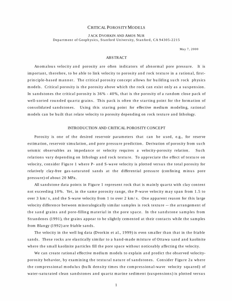
1

CRITICAL POROSITY MODELS

JACK DVORKIN AND AMOS NURDepartment of Geophysics, Stanford University, Stanford, CA 94305-2215

May 7, 2000

ABSTRACT

Anomalous velocity and porosity are often indicators of abnormal pore pressure. It is

important, therefore, to be able to link velocity to porosity and rock texture in a rational, first-

principle-based manner. The critical porosity concept allows for building such rock physics

models. Critical porosity is the porosity above which the rock can exist only as a suspension.

In sandstones the critical porosity is 36% - 40%, that is the porosity of a random close pack of

well-sorted rounded quartz grains. This pack is often the starting point for the formation of

consolidated sandstones. Using this staring point for effective medium modeling, rational

models can be built that relate velocity to porosity depending on rock texture and lithology.

INTRODUCTION AND CRITICAL POROSITY CONCEPT

Porosity is one of the desired reservoir parameters that can be used, e.g., for reserve

estimation, reservoir simulation, and pore pressure prediction. Derivation of porosity from such

seismic observables as impedance or velocity requires a velocity-porosity relation. Such

relations vary depending on lithology and rock texture. To appreciate the effect of texture on

velocity, consider Figure 1 where P- and S-wave velocity is plotted versus the total porosity for

relatively clay-free gas-saturated sands at the differential pressure (confining minus pore

pressure) of about 20 MPa.

All sandstone data points in Figure 1 represent rock that is mainly quartz with clay content

not exceeding 10%. Yet, in the same porosity range, the P-wave velocity may span from 1.5 to

over 3 km/s, and the S-wave velocity from 1 to over 2 km/s. One apparent reason for this large

velocity difference between mineralogically similar samples is rock texture -- the arrangement of

the sand grains and pore-filling material in the pore space. In the sandstone samples from

Strandenes (1991), the grains appear to be slightly cemented at their contacts while the samples

from Blangy (1992) are friable sands.

The velocity in the well log data (Dvorkin et al., 1999) is even smaller than that in the friable

sands. These rocks are elastically similar to a hand-made mixture of Ottawa sand and kaolinite

where the small kaolinite particles fill the pore space without noticeably affecting the velocity.

We can create rational effective medium models to explain and predict the observed velocity-

porosity behavior, by examining the textural nature of sandstones. Consider Figure 2a where

the compressional modulus (bulk density times the compressional-wave velocity squared) of

water-saturated clean sandstones and quartz marine sediment (suspensions) is plotted versus

2

porosity. The porosity of 36 - 40% is the point where the modulus-porosity trend abruptly

changes. In the lower porosity domain, the stiffness of the sandstone is determined by the

framework of contacting quartz grains. In the higher-porosity domain, the grains are not in

contact anymore and are suspended in water. In this case, the stiffness of the sediment is

determined by the pore fluid.

1.5

2

3

4

0.2 0.3 0.4

Vp (km

/s)

Porositya

Ottawa+Clay

Strandenes

Blangy

WellLog

1

2

0.2 0.3 0.4

Vs

(km

/s)

Porosityb

Figure 1. P- and S-wave velocity in rocks with gas at 20 MPa differential pressure. Circles

represent laboratory data obtained on high-porosity "fast" (Strandenes, 1991) and "slow" (Blangy,

1992) sands, both data sets are from the North Sea. Gray symbols are from a Gulf Coast gas well.

The filled square is for a hand-made mixture of Ottawa sand and 10% kaolinite (Yin, 1993). Clay

content for these data does not exceed 10%.

0

20

40

60

80

0 0.2 0.4 0.6 0.8 1

Ela

stic

Mod

uli

(GPa)

Porositya

Quartz

CompressionalModulus

Suspension

0 0.1 0.2 0.3 0.4

Porosityb

CompressionalModulus

ShearModulus

Figure 2. a. Compressional modulus versus porosity in clean sandstones and marine sediment

versus porosity. b. Compressional and shear modulus of sandstones versus porosity. The data

used are discussed in Nur et al. (1998).

We call this threshold porosity "critical porosity" (Nur et al., 1998). The rocks where the

solid phase is spatially continuous and dominates the stiffness of the rock have porosity that is

smaller than the critical porosity. This fact is illustrated in Figure 2b where the compressional

and shear moduli of many sandstone samples (room-dry at 30 - 40 MPa differential pressure) are

plotted versus porosity.

3

The critical porosity concept is valid not only for sandstones but also for other natural and

artificial rocks. An example is given in Figure 3 where the compressional modulus is plotted

versus porosity for cracked igneous rocks and pumice (Nur et al., 1998). In the first case, the

critical porosity is as small as 6% while in the second case it reaches 70%. The reason is the

peculiar microstructural topology of the rocks under examination. The igneous rocks are

permeated by cracks that percolate and make the solid phase loose its spatial continuity at very

small porosity. In the pumice, the honeycomb structure of the solid ensures its spatial

continuity at high porosity values.

0

20

40

60

80

0 0.2 0.4 0.6 0.8 1

Com

pre

ssio

nal

Mod

ulu

s (G

Pa)

Porosity

CrackedIgneous Rocks

withPercolating

Cracks

Pumicewith

HoneycombStructure

Figure 3. Compressional modulus versus porosity in cracked igneous rocks and pumice. The data

used are discussed in Nur et al. (1998).

Nur et al. (1998) summarize the critical porosity values for various rocks as follows:

Material Critical PorositySandstones 40%Limestones 40%Dolomites 40%Pumice 80%Chalks 65%

Rock Salt 40%Cracked Igneous Rocks 5%

Oceanic Basalts 20%Sintered Glass Beads 40%

Glass Foam 90%

Below, we introduce the critical concentration concept, and describe several effective

medium models that are based on the critical porosity concept.

CRITICAL CONCENTRATION CONCEPT

The critical porosity concept leads to the "critical concentration" concept that Marion (1990)

and Yin (1993) used to describe the properties of sands with shale. Consider the experimental

data from Yin (1993) obtained on synthetic rocks made by mixing Ottawa sand and kaolinite.

The volumetric clay content in the samples varied from 0 to 100%.

4

The total porosity at 20 MPa differential pressure is plotted versus the volumetric clay

content in Figure 4a. The two end members of the data set are the porosity of Ottawa sand at

zero clay content and porosity of kaolinite at 100% clay content. The porosity of the mixture

reaches its minimum at the point where the volumetric concentration of clay equals the

porosity of Ottawa sand (which is close to the critical porosity for sandstones). This clay

content is called "critical clay concentration."

The critical concentration affects not only for the total porosity but also the dynamic

(velocity-derived) elastic moduli of the mixture (Figure 4b). The elastic moduli of the mixture are

maximum at the critical concentration and decrease as the clay content increases or decreases

from the critical concentration value. Poisson's ratio behaves in a similar way (Figure 4c).

0.2

0.3

0.4

0.5

0 0.2 0.4 0.6 0.8 1

Tot

al P

oros

ity

Clay Content Volume

Ottawa + Kaolinite

a

1

2

3

4

5

6

0 0.2 0.4 0.6 0.8 1

Ela

stic

Mod

uli

(GPa)

Clay Content Volume

CompressionalModulus

ShearModulus

b

.2

.3

0 0.2 0.4 0.6 0.8 1Poi

sson

's R

atio

Clay Content Volumec

Figure 4. Porosity (a), elastic moduli (b), and Poisson's ratio (c) versus volumetric clay content in

room-dry Ottawa sand mixed with kaolinite at 20 MPa differential pressure (after Yin, 1993).

The elastic properties of the synthetic mixture of Ottawa sand and kaolinite are plotted

versus the total porosity in Figure 5. The non-uniqueness of the elastic moduli, and, especially,

Poisson's ratio in the cross-plots is due to the grain-scale texture of the rock.

This effect has to be considered when examining well-log data. In Figure 6a and 6b, we plot

the bulk density and P-wave impedance versus the gamma-ray values for a well in Colombia

(Gutierrez, 1998). Different trends are apparent for the low-gamma-ray and the high-gamma-ray

branches. This effect depends on the rock's microstructure and results in non-uniqueness as

the P-wave impedance is plotted versus the bulk density and porosity (Figure 6c and 6d). Being

aware of the physical reason underlying these non-unique cross-plots will allow the log analyst

to separate the trends and arrive at accurate impedance-porosity transforms.

5

1

2

3

4

5

6

0.20 0.25 0.30 0.35

Ela

stic

Mod

uli

(GPa)

Total Porosity

CompressionalModulus

ShearModulus

a

.2

.3

0.20 0.25 0.30 0.35

Poi

sson

's R

atio

Total Porosityb

Figure 5. Elastic moduli (a) and Poisson's ratio (b) versus total porosity in room-dry Ottawa

sand mixed with kaolinite at 20 MPa differential pressure (after Yin, 1993). The arrows

show increasing clay content.

2.1

2.2

2.3

2.4

2.5

50 75 100 125 150 175

Bu

lk D

ensi

ty

GRa

GR < 115GR > 115

5

6

7

8

9

50 75 100 125 150 175

P-I

mped

ance

GRb

5

6

7

8

9

2.1 2.2 2.3 2.4 2.5

P-I

mped

ance

Bulk Densityc

GR < 115GR > 115

5

6

7

8

9

0.1 0.2 0.3

P-I

mped

ance

Total Porosityd

Figure 6. Well log data. Bulk density and P-impedance versus gamma-ray (a and b); P-

impedance versus bulk density and total porosity (c and d).

MODELS FOR HIGH-POROSITY SANDSTONES

The initial building point for effective medium models that describe high-porosity

6

sandstones should be unconsolidated well-sorted sand, as proposed by the critical

porosity concept. In mathematical modeling, such sand is approximated by a dense

pack of identical elastic spheres (Figure 7).

Figure 7. Approximating sand by a sphere pack (microphotographs of well-sorted sand,

left, and a glass-bead pack, right).

The contact-cement model (Dvorkin and Nur, 1996) assumes that porosity decreases

from the initial critical porosity value due to the uniform deposition of cement layers on

the surface of the grains. This cement may be diagenetic quartz, calcite, or reactive clay

(such as illite). The diagenetic cement dramatically increases the stiffness of the sand by

reinforcing the grain contacts (Figure 8). The mathematical model is based on a rigorous

contact-problem solution by Dvorkin et al. (1994).

0.30 0.35 0.40

Ela

stic

Mod

ulu

s

Porositya

ContactCementModel

0.30 0.35 0.40Porosityb

Friable SandModel

0.30 0.35 0.40Porosity

ConstantCementModel

c

Figure 8. Schematic depiction of three effective-medium models for high-porosity

sandstones and corresponding diagenetic transformations.

In this model, the effective bulk ( Kdry ) and shear (Gdry ) moduli of dry rock are:

Kdry = n(1 − φc )McSn / 6, Gdry = 3Kdry / 5 + 3n(1 − φc )GcSτ / 20, (1)

where φc is critical porosity; Ks and Gs are the bulk and shear moduli of the grain

material, respectively; Kc and Gc are the bulk and shear moduli of the cement material,

respectively; Mc = Kc + 4Gc / 3 is the compressional modulus of the cement; and n is

7

the coordination number -- average number of contacts per grain (8-9). Sn and Sτ are:

Sn = An(Λn )α 2 + Bn (Λn )α + Cn (Λn), An (Λn ) = −0.024153 ⋅Λ n−1.3646,

Bn (Λn ) = 0.20405 ⋅Λ n−0.89008, Cn (Λn ) = 0.00024649 ⋅Λ n

−1.9864;Sτ = Aτ (Λτ , νs )α

2 + Bτ (Λτ , νs )α + Cτ (Λτ , νs ),

Aτ(Λτ ,νs ) = −10−2 ⋅ (2.26νs2 + 2.07νs + 2.3) ⋅Λ τ

0.079νs2 + 0.1754νs −1.342,

Bτ (Λτ ,νs ) = (0.0573νs2 + 0.0937νs + 0.202) ⋅Λ τ

0.0274ν s2 +0.0529νs − 0.8765,

Cτ (Λτ ,νs ) = 10−4 ⋅(9.654νs2 + 4.945νs + 3.1) ⋅Λ τ

0.01867νs2 + 0.4011ν s −1.8186;

Λn = 2Gc (1− νs )(1− νc) /[ πGs (1− 2νc )], Λτ = Gc / (πGs );

α = [(2 / 3)(φc − φ ) / (1− φc )]0.5;νc = 0.5(Kc / Gc − 2 / 3)/ (Kc / Gc +1/ 3);νs = 0.5(Ks / Gs − 2 / 3)/ (Ks / Gs +1/ 3).

A detailed explanation of these equations and their derivation are given in Dvorkin and

Nur (1996).

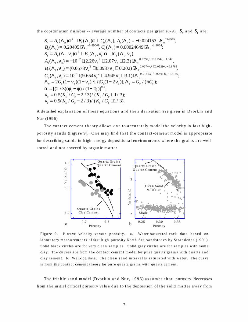
The contact cement theory allows one to accurately model the velocity in fast high-

porosity sands (Figure 9). One may find that the contact-cement model is appropriate

for describing sands in high-energy depositional environments where the grains are well-

sorted and not covered by organic matter.

3.0

3.5

4.0

0.2 0.3

Vp (km

/s)

Porosity

Quartz GrainsQuartz Cement

Quartz GrainsClay Cement

a

2

3

0.25 0.30 0.35

Vp (km

/s)

Porosity

Clean Sandw/Water

b

Quartz GrainsQuartz Cement

Shale

Figure 9. P-wave velocity versus porosity. a. Water-saturated-rock data based on

laboratory measurements of fast high-porosity North Sea sandstones by Strandenes (1991).

Solid black circles are for very clean samples. Solid gray circles are for samples with some

clay. The curves are from the contact cement model for pure quartz grains with quartz and

clay cement. b. Well-log data. The clean sand interval is saturated with water. The curve

is from the contact cement theory for pure quartz grains with quartz cement.

The friable sand model (Dvorkin and Nur, 1996) assumes that porosity decreases

from the initial critical porosity value due to the deposition of the solid matter away from

8

the grain contacts. Such a diagenetic process of porosity reduction may correspond to

deteriorating grain sorting. This non-contact additional solid matter weakly affects the

stiffness of the rock (Figure 8b).

The theoretical effective-medium model connects two end-points in the elastic-

modulus-porosity plane. One end point is at critical porosity. The elastic moduli of the

dry rock at that point are assumed to be the same as of an elastic sphere pack subject to

confining pressure. These moduli are given by the Hertz-Mindlin (Mindlin, 1949) theory:

KHM = [n2 (1− φc)

2 G2

18π 2(1− ν)2 P]1

3 , GHM =5 − 4ν

5(2 − ν )[3n2 (1− φc)

2 G2

2π 2(1− ν)2 P]1

3 ; (2)

where KHM and GHM are the bulk and shear moduli at critical porosity φc , respectively;

P is the differential pressure; K , G , and ν are the bulk and shear moduli of the solid

phase, and its Poisson's ratio, respectively; and n is the coordination number.

The other end-point is at zero porosity and has the bulk ( K ) and shear (G ) moduli

of the pure solid phase. These two points in the porosity-moduli plane are connected

with the curves that have the algebraic expressions of the lower Hashin-Shtrikman

(1963) bound (bulk and shear moduli) for the mixture of two components: the pure

solid phase and the phase that is the sphere pack. The reasoning is that in

unconsolidated sediment, the softest component (the sphere pack) envelopes the stiffest

component (the solid) in the Hashin-Shtrikman fashion (Figure 10).

At porosity φ the concentration of the pure solid phase (added to the sphere pack to

decrease porosity) in the rock is 1 − φ / φc and that of the sphere-pack phase is φ / φc .

Then the bulk ( KDry ) and shear (GDry ) moduli of the dry frame are:

KDry = [φ / φc

KHM + 43 GHM

+1 − φ / φc

K + 43 GHM

]−1 −4

3GHM ,

GDry = [ φ / φc

GHM + z+ 1 − φ / φc

G + z]−1 − z, z = GHM

69KHM + 8GHM

KHM + 2GHM

.

(3)

φ < φc φ = φc φ >φc φ =1φ =0

Increasing Porosity

Figure 10. Hashin-Shtrikman arrangements of sphere pack, solid, and void.

The friable sand model allows one to accurately predict velocity in soft high-porosity

sands (Figure 11). This model is appropriate for describing sands where contact cement

9

deposition was inhibited by organic matter deposited on the grain surface.

1

2

3

0.2 0.3 0.4

Vel

ocit

y (k

m/s

)

Porositya

Vp

Vs

2

3

0.30 0.35 0.40

Vp (km

/s)

Porosityb

Figure 11. Velocity versus porosity. a. Water-saturated-rock data based on laboratory

measurements of soft high-porosity North Sea sandstones by Blangy (1992). b. Well-log

data (Avseth et al., 1998) for oil-saturated pay zone. The curves are from the friable sand

model.

The constant-cement model (Avseth et al., 1998) assumes that the initial porosity

reduction from critical porosity is due to the contact cement deposition. At some high

porosity, this diagenetic process stops and after that porosity reduces due to the

deposition of the solid phase away from the grain contacts as in the friable sand model

(Figure 8c). This model is mathematically analogous to the friable sand model except

that the high-porosity end point bulk and shear moduli ( Kb and Gb , respectively) are

calculated at some "cemented" porosity φb from the contact-cement model. Then the

dry-rock bulk and shear moduli are:

Kdry = (φ / φb

Kb + 4Gb / 3+

1 − φ / φb

Ks + 4Gb / 3)−1 − 4Gb / 3,

Gdry = (φ / φb

Gb + z+

1 − φ / φb

Gs + z)−1 − z, z =

Gb

6

9Kb + 8Gb

Kb + 2Gb

.(4)

An example of applying this model to well-log data is given in Figure 12.

2.8

3.0

3.2

3.4

0.2 0.3 0.4

Vp (km

/s)

Porosity

10

Figure 12. Velocity versus porosity. Well-log data (Avseth et al., 1998) for oil-saturated

pay zone. The curve is from the constant cement model.

MODELS FOR UNCONSOLIDATED MARINE SEDIMENT

This model (Dvorkin et al., 1999) is analogous to the friable sand model but covers

the porosity range above critical porosity. One end point is the critical porosity where

the elastic moduli of the sphere pack are given by Equations (2). To arrive at higher

porosity, we add empty voids to the sphere pack (Figure 10). In this case the voids are

placed inside the pack in the Hashin-Shtrikman fashion. Now the pack is the stiffest

component, so we have to use the upper Hashin-Shtrikman limit.

At porosity φ > φc , the concentration of the void phase is (φ − φc )/ (1− φc ) and that

of the sphere-pack phase is (1− φ )/ (1− φc ) . Then the effective dry-rock frame bulk and

shear moduli are:

KDry = [ (1 − φ )/(1 − φc )KHM + 4

3 GHM

+ (φ − φc )/(1 − φc )43 GHM

]−1 − 4

3GHM,

GDry = [(1 − φ )/(1 − φc )

GHM + z+

(φ − φc )/(1 − φc )z

]−1 − z,

z =GHM

6

9KHM + 8GHM

KHM + 2GHM

.

(5)

The saturated-rock elastic moduli can be calculated using Gassmann's (1951)

equation.

An example of applying this model to log data is given in Figure 13 (Dvorkin et al,

1999). A good agreement between the model and the data is apparent. At the same

time, the often used suspension model fails to correctly mimic the data. This model's

departure from the data increases with depth which is due to the effect of confining

pressure that adds stiffness to the dry frame of the sediment thus making the

suspension model inadequate.

11

0.5 0.55 0.6 0.65

60

80

100

120

Neutron Porosity

Dep

th (m

bsf

)

a 1.5 1.6 1.7 1.8P-Wave Velocity (km/s)

DataThis ModelSuspension

b

Figure 13. DSDP Well 974. a. Neutron porosity versus depth. b. Velocity versus depth:

data, our model, and suspension model. All curves are smoothed.

CONCLUSION

The critical porosity and critical concentration concepts allow the geophysicist to

better understand the diversity of well log and core elastic data. Effective-medium

models built on the basis of the critical porosity concept can accurately model data. By

superimposing theoretical model curves on velocity-porosity and elastic-moduli-porosity

crossplots, one may mathematically diagnose rock, i.e., determine the texture of the

sediment (e.g., contact-cemented versus friable). Rock physics diagnostic can be

conducted with velocity, impedance, or elastic moduli. Examples of diagnostic rock

curves are given in Figure 14. Such diagnostic curves have implications for fluid

detection (Avseth et al., 1998), and strength and permeability (Dvorkin and Brevik,

1999). Moreover, the rock physics diagnostic may be crucial for pore pressure prediction

from velocity because at the same pressure, velocity may vary depending on rock texture

(Dvorkin et al, 1999). As a result, texture-related velocity variations may be mistakenly

attributed to pore pressure anomalies.

3

4

0.2 0.3 0.4

Vp (km

/s)

Porositya

Cement Quartz

CementClay

FriableSand

2.5

3.0

0.3 0.35 0.4

Vp (km

/s)

Porosityb

ContactCement

ConstantCement

FriableSand

12

Figure 14. Velocity versus porosity. Theoretical curves superimposed on data allow one to

identify the rock type. a. Data from Figures 9a and 11a. b. Data from Figures 11b and 12.

ACKNOWLEDGMENT

This work was supported by the Stanford Rock Physics Laboratory.

REFERENCES

Strandenes, S., 1991, Rock physics analysis of the Brent Group reservoir in the Oseberg

Field: Unpublished Data.

Blangy, J.P., 1992, Integrated seismic lithologic interpretation: The petrophysical basis:

Ph.D. thesis, Stanford University.

Dvorkin, J., Moos, D., Packwood, J., and Nur, A., 1999, Identifying patchy saturation

from well logs: Geophysics, 64 1-5.

Yin, H., 1993, Acoustic velocity and attenuation of rocks: isotropy, intrinsic anisotropy,

and stress induced anisotropy: Ph.D. thesis, Stanford University.

Nur, A., Mavko, G., Dvorkin, J., and Galmudi, D., 1998, Critical Porosity: A Key to

Relating Physical Properties to Porosity in Rocks, The Leading Edge, 17, 357-362.

Marion, D., 1990, Acoustical, mechanical, and transport properties of sediments and

granular materials: Ph.D. thesis, Stanford University.

Gutierrez, M., 1998, personal communication.

Dvorkin, J., and Nur, A., 1996, Elasticity of High-Porosity Sandstones: Theory for Two

North Sea Datasets, Geophysics, 61, 1363-1370.

Dvorkin, J., Nur, A., and Yin, H., 1994, Effective Properties of Cemented Granular

Materials, Mechanics of Materials, 18, 351-366.

Mindlin, R.D., 1949, Compliance of elastic bodies in contact, J. Appl. Mech., 16, 259-

268.

Hashin, Z., and Shtrikman, S., 1963, A variational approach to the elastic behavior of

multiphase materials: J. Mech. Phys. Solids, 11, 127-140.

Avseth, P., Dvorkin, J., Mavko, G., and Rykkje, J., 1998, Diagnosing high-porosity sands

for reservoir characterization using sonic and seismic, SEG 66 Annual Meeting,

Expanded Abstracts, 1024-1025.

Dvorkin, J., Prasad, M., Sakai, A., and Lavoie, D., 1999, Elasticity of marine sediments,

GRL, 26, 1781-1784.

Dvorkin, J., and Brevik, I., 1999, Diagnosing high-porosity sandstones: Strength and

permeability from porosity and velocity, Geophysics, 64, 795-799.

Dvorkin, J., Mavko, G., and Nur, A., 1999, Overpressure detection from compressional-

and shear-wave data, GRL, 26, 3417-3420.