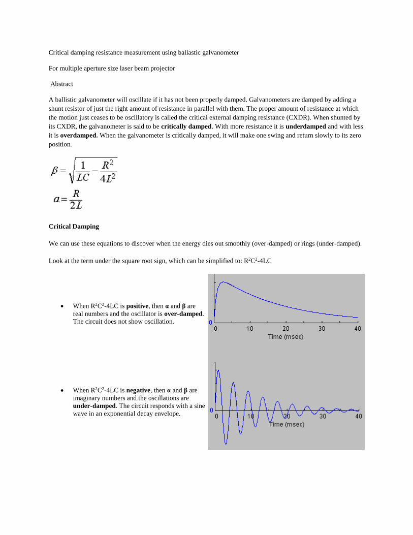
Critical damping resistance measurement using ballastic galvanometer

For multiple aperture size laser beam projector

Abstract

A ballistic galvanometer will oscillate if it has not been properly damped. Galvanometers are damped by adding a

shunt resistor of just the right amount of resistance in parallel with them. The proper amount of resistance at which

the motion just ceases to be oscillatory is called the critical external damping resistance (CXDR). When shunted by

its CXDR, the galvanometer is said to be critically damped. With more resistance it is underdamped and with less

it is overdamped. When the galvanometer is critically damped, it will make one swing and return slowly to its zero

position.

Critical Damping

We can use these equations to discover when the energy dies out smoothly (over-damped) or rings (under-damped).

Look at the term under the square root sign, which can be simplified to: R2C2-4LC

When R2C2-4LC is positive, then α and β are

real numbers and the oscillator is over-damped.

The circuit does not show oscillation.

When R2C2-4LC is negative, then α and β are

imaginary numbers and the oscillations are

under-damped. The circuit responds with a sine

wave in an exponential decay envelope.

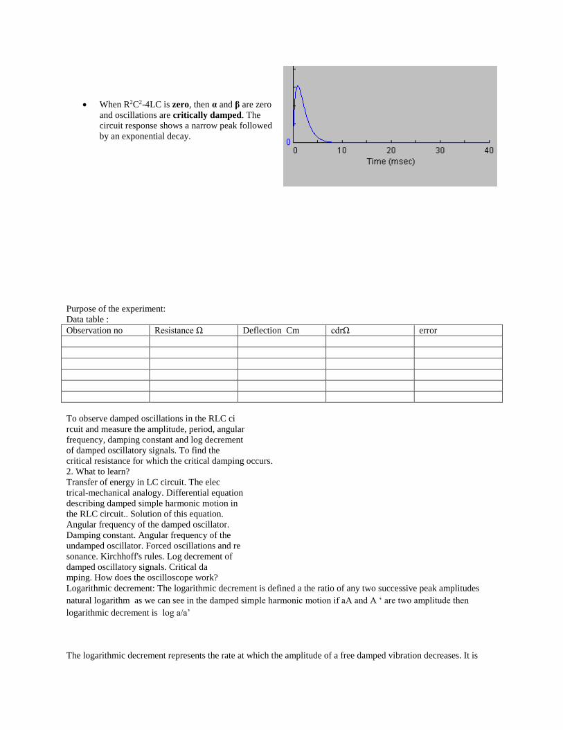
When R2C2-4LC is zero, then α and β are zero

and oscillations are critically damped. The

circuit response shows a narrow peak followed

by an exponential decay.

Purpose of the experiment:

Data table :

Observation no Resistance Ω Deflection Cm cdrΩ error

To observe damped oscillations in the RLC ci

rcuit and measure the amplitude, period, angular

frequency, damping constant and log decrement

of damped oscillatory signals. To find the

critical resistance for which the critical damping occurs.

2. What to learn?

Transfer of energy in LC circuit. The elec

trical-mechanical analogy. Differential equation

describing damped simple harmonic motion in

the RLC circuit.. Solution of this equation.

Angular frequency of the damped oscillator.

Damping constant. Angular frequency of the

undamped oscillator. Forced oscillations and re

sonance. Kirchhoff's rules. Log decrement of

damped oscillatory signals. Critical da

mping. How does the oscilloscope work?

Logarithmic decrement: The logarithmic decrement is defined a the ratio of any two successive peak amplitudes

natural logarithm as we can see in the damped simple harmonic motion if aA and A ‘ are two amplitude then

logarithmic decrement is log a/a’

The logarithmic decrement represents the rate at which the amplitude of a free damped vibration decreases. It is

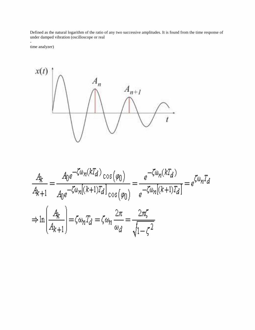
Defined as the natural logarithm of the ratio of any two successive amplitudes. It is found from the time response of

under damped vibration (oscilloscope or real

-

time analyzer)

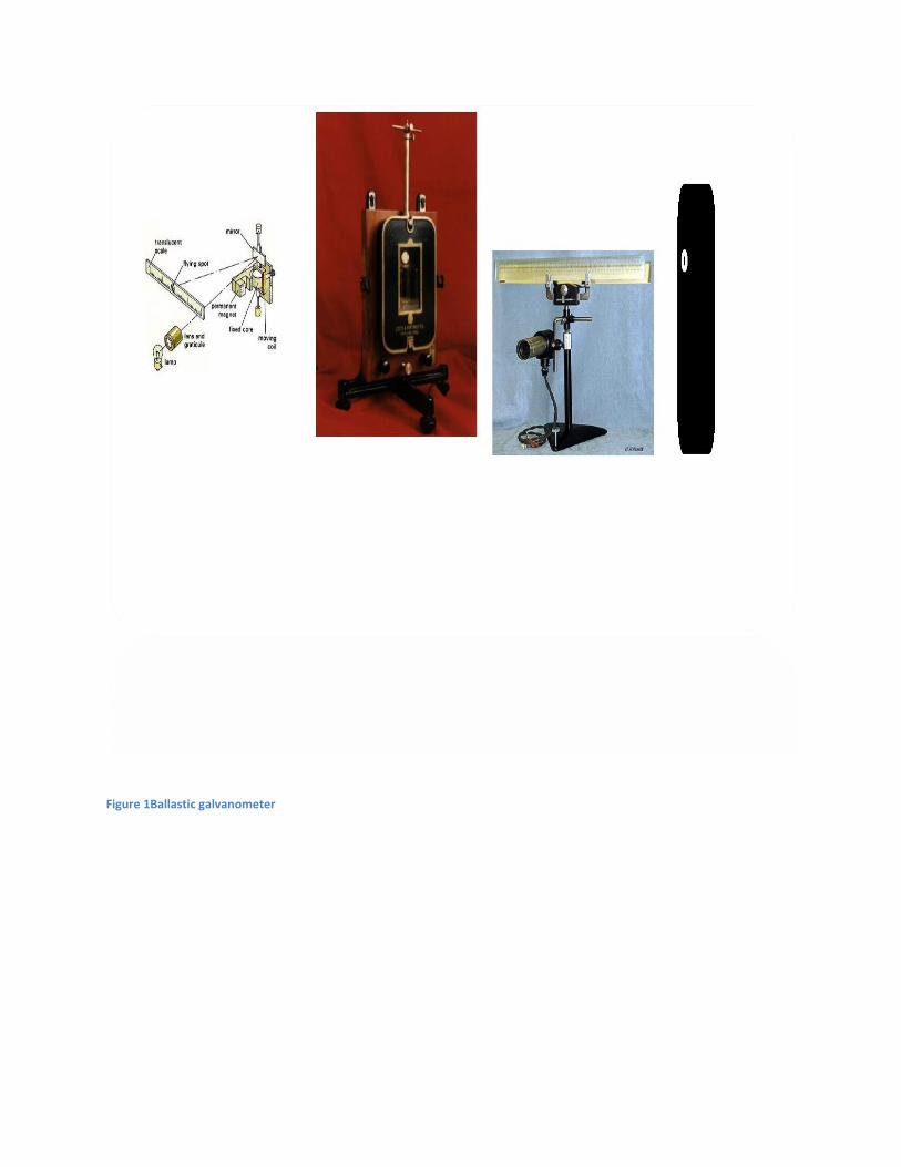
Figure 1Ballastic galvanometer

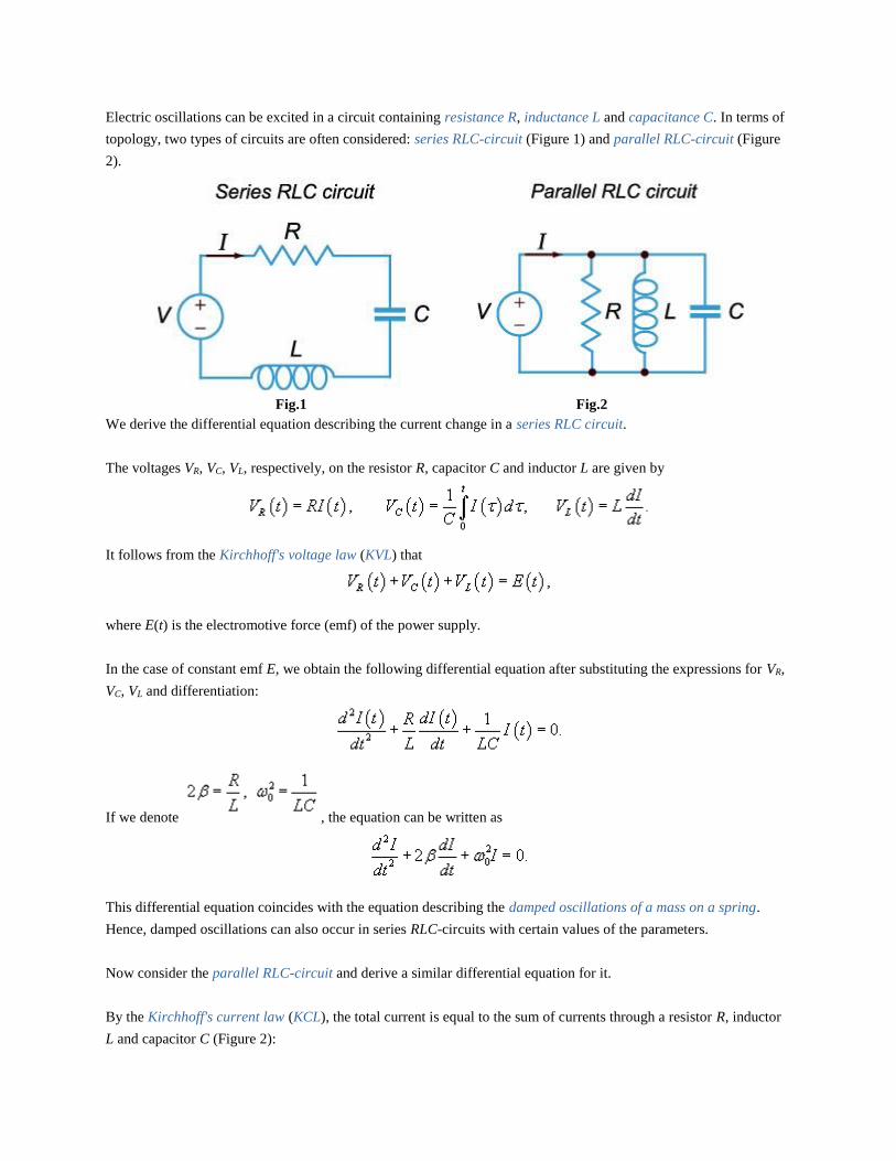
Electric oscillations can be excited in a circuit containing resistance R, inductance L and capacitance C. In terms of

topology, two types of circuits are often considered: series RLC-circuit (Figure 1) and parallel RLC-circuit (Figure

2).

Fig.1

Fig.2

We derive the differential equation describing the current change in a series RLC circuit.

The voltages VR, VC, VL, respectively, on the resistor R, capacitor C and inductor L are given by

It follows from the Kirchhoff's voltage law (KVL) that

where E(t) is the electromotive force (emf) of the power supply.

In the case of constant emf E, we obtain the following differential equation after substituting the expressions for VR,

VC, VL and differentiation:

If we denote , the equation can be written as

This differential equation coincides with the equation describing the damped oscillations of a mass on a spring.

Hence, damped oscillations can also occur in series RLC-circuits with certain values of the parameters.

Now consider the parallel RLC-circuit and derive a similar differential equation for it.

By the Kirchhoff's current law (KCL), the total current is equal to the sum of currents through a resistor R, inductor

L and capacitor C (Figure 2):

Given that

For the case of constant total current I(t) = I0, we obtain the following differential equation of the second order with

respect to the variable V:

As one can see, we again have the equation describing the damped oscillations. Thus, the oscillatory mode can also

occur in parallel RLC-circuits.

Resonant Circuit. Thomson Formula

In the simplest case, when the ohmic resistance is zero (R = 0) and the source of emf is removed (E = 0), the

resonant circuit consists only of a capacitor C and inductor L, and is described by the differential equation

In this circuit there will be undamped electrical oscillations with a period

This formula is called the Thomson formula in honor of British physicist William Thomson (1824-1907), who

derived it theoretically in 1853.

Damped Oscillations in Series RLC-Circuit

The second order differential equation describing the damped oscillations in a series RLC-circuit we got above can

be written as

The corresponding characteristic equation has the form

Its roots are calculated by the formulas:

where the value of β = R/2L is called the damping coefficient, and ω0 is the resonant frequency of the resonant

circuit.

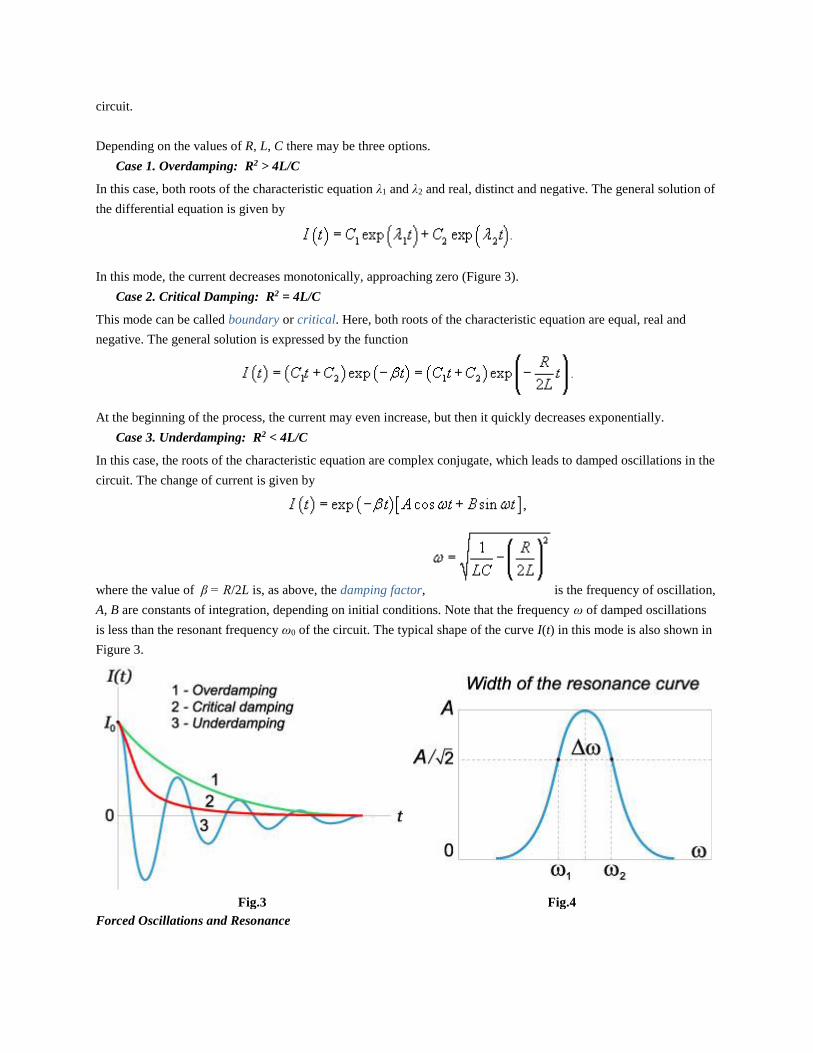
Depending on the values of R, L, C there may be three options.

Case 1. Overdamping: R2 > 4L/C

In this case, both roots of the characteristic equation λ1 and λ2 and real, distinct and negative. The general solution of

the differential equation is given by

In this mode, the current decreases monotonically, approaching zero (Figure 3).

Case 2. Critical Damping: R2 = 4L/C

This mode can be called boundary or critical. Here, both roots of the characteristic equation are equal, real and

negative. The general solution is expressed by the function

At the beginning of the process, the current may even increase, but then it quickly decreases exponentially.

Case 3. Underdamping: R2 < 4L/C

In this case, the roots of the characteristic equation are complex conjugate, which leads to damped oscillations in the

circuit. The change of current is given by

where the value of β = R/2L is, as above, the damping factor, is the frequency of oscillation,

A, B are constants of integration, depending on initial conditions. Note that the frequency ω of damped oscillations

is less than the resonant frequency ω0 of the circuit. The typical shape of the curve I(t) in this mode is also shown in

Figure 3.

Fig.3

Fig.4

Forced Oscillations and Resonance

If the resonant circuit includes a generator with periodically varying emf, the forced oscillations arise in the system.

If the emf E of the source varies according to the law

then the differential equation of forced oscillations in series RLC-circuit can be written as

where q the charge of the capacitor, .

This equation is analogous to the equation of forced oscillations of a spring pendulum, discussed on the page

Mechanical Oscillations. Its general solution is the sum of two components: the general solution of the associated

homogeneous equation and a particular solution of the nonhomogeneous equation. The first component describes the

decaying transient process, after which the behavior of the system depends only on the external driving force. The

forced oscillations will occur according to the law

where the phase φ is determined by the formula

Knowing the change of the charge q(t), it is easy to find the change of the current I(t):

where we have introduced the angle θ such that . The angle indicates the phase

shift of the current oscillations I(t) with respect to oscillations in the supply voltage .

The amplitude of the current I0 and the phase shift θ are given by

The quantity is called the impedance, or impedance of the circuit. It consists of an

ohmic resistance R and a reactance . Impedance of the resonant circuit in the complex form can be

written as

We see from these formulas that the amplitude of steady-state oscillations of the current is maximum when

Resonance in the resonant circuit appears under this condition. The resonant frequency ω0 is equal to the frequency

of free oscillations in the circuit and does not depend on the resistance R.

We can transform the formula for the amplitude of the forced oscillations to get an explicit dependence on the

frequency ratio ω/ω0, where ω0 is the resonant frequency. As a result, we obtain

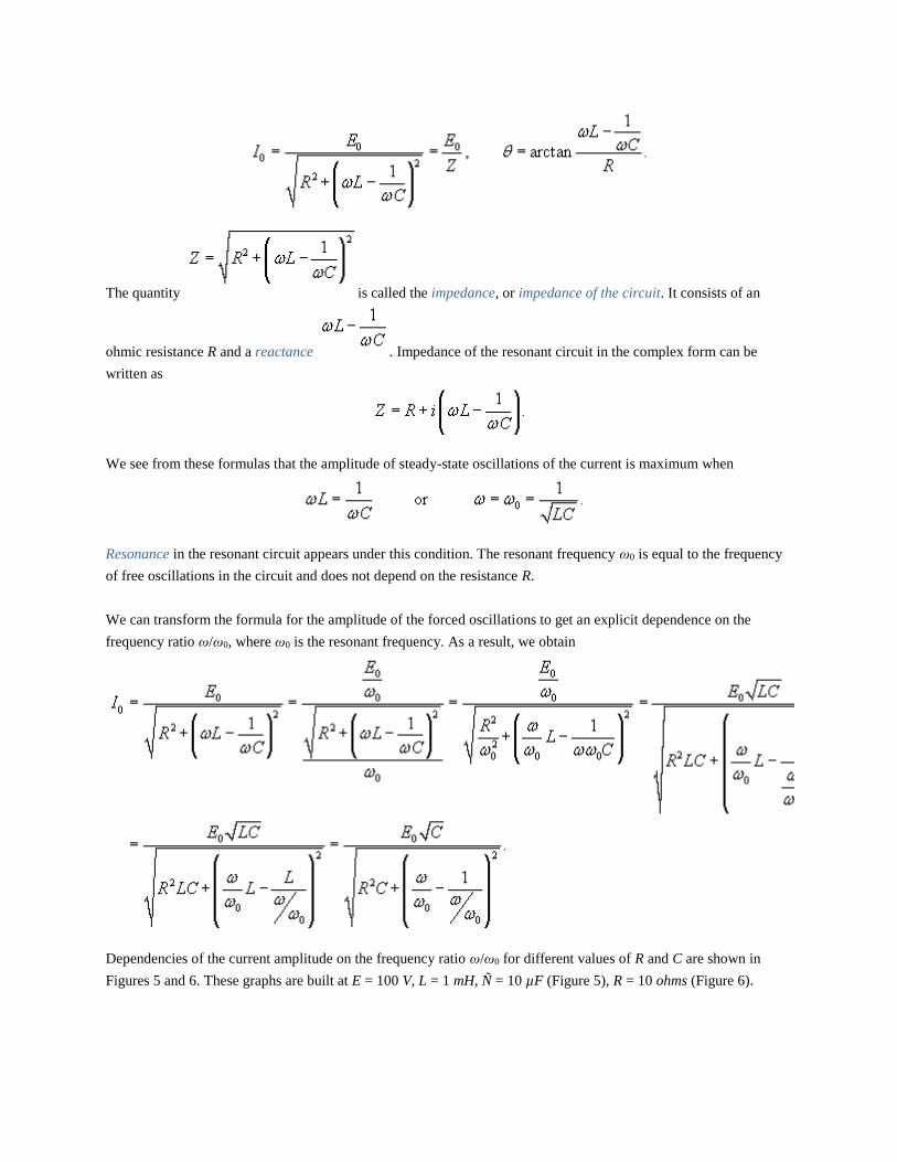
Dependencies of the current amplitude on the frequency ratio ω/ω0 for different values of R and C are shown in

Figures 5 and 6. These graphs are built at E = 100 V, L = 1 mH, Ñ = 10 µF (Figure 5), R = 10 ohms (Figure 6).

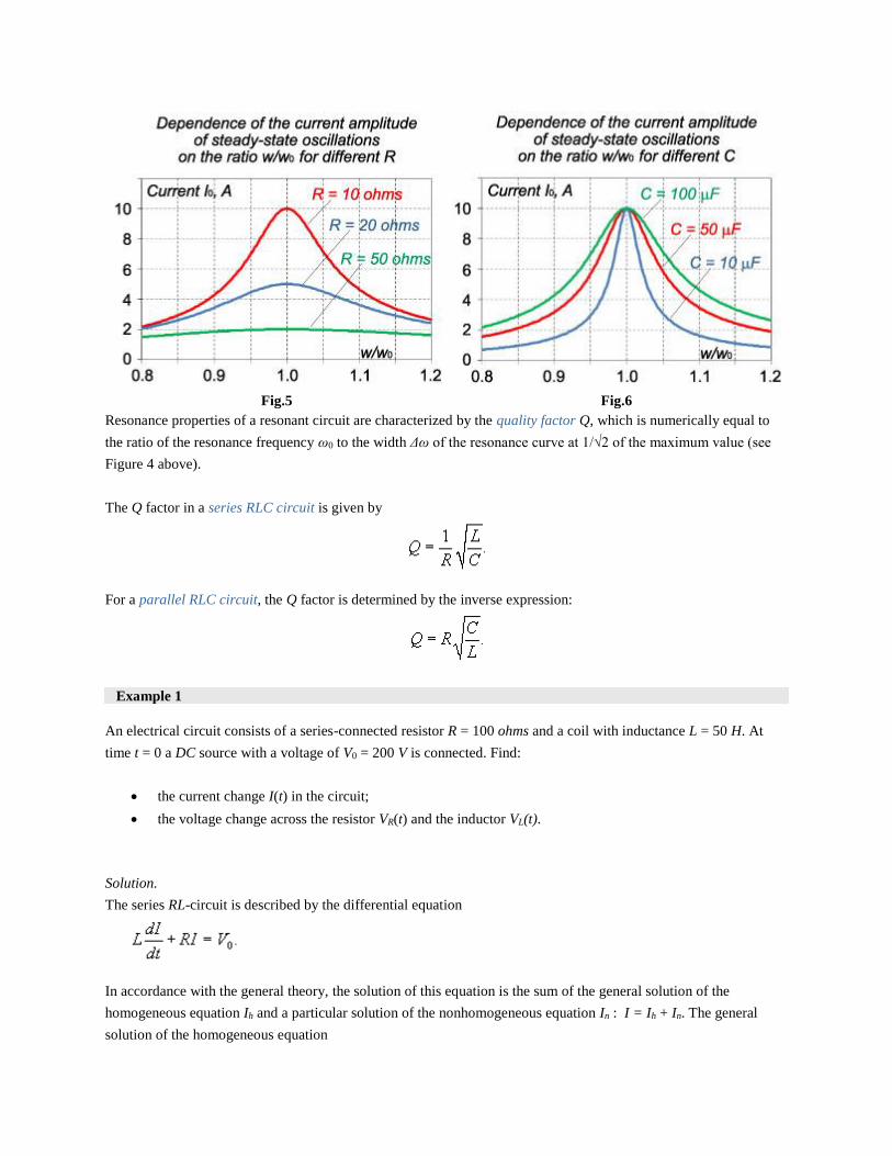
Fig.5

Fig.6

Resonance properties of a resonant circuit are characterized by the quality factor Q, which is numerically equal to

the ratio of the resonance frequency ω0 to the width Δω of the resonance curve at 1/√2 of the maximum value (see

Figure 4 above).

The Q factor in a series RLC circuit is given by

For a parallel RLC circuit, the Q factor is determined by the inverse expression:

Example 1

An electrical circuit consists of a series-connected resistor R = 100 ohms and a coil with inductance L = 50 H. At

time t = 0 a DC source with a voltage of V0 = 200 V is connected. Find:

the current change I(t) in the circuit;

the voltage change across the resistor VR(t) and the inductor VL(t).

Solution.

The series RL-circuit is described by the differential equation

In accordance with the general theory, the solution of this equation is the sum of the general solution of the

homogeneous equation Ih and a particular solution of the nonhomogeneous equation In : I = Ih + In. The general

solution of the homogeneous equation

is expressed as

where A is the constant of integration.

The solution of the nonhomogeneous equation In corresponds to the steady state in which the current in the circuit is

determined only by the ohmic resistance R: . Then the total current varies according to the law

The constant A is determined from the initial condition I(t = 0) = 0. Consequently,

So, after the circuit is closed, the current will vary according to the law

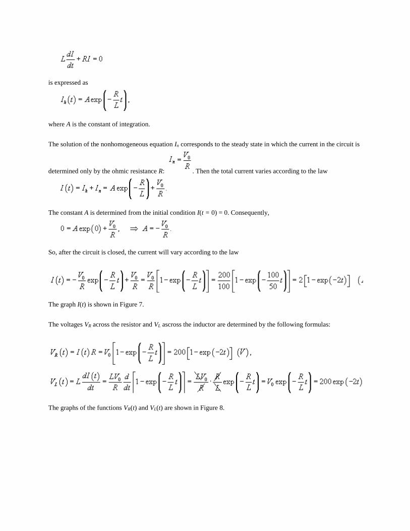
The graph I(t) is shown in Figure 7.

The voltages VR across the resistor and VL ascross the inductor are determined by the following formulas:

The graphs of the functions VR(t) and VL(t) are shown in Figure 8.

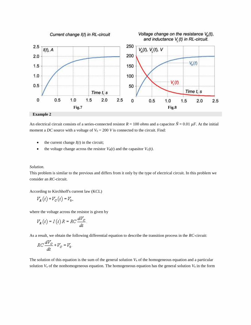
Fig.7

Fig.8

Example 2

An electrical circuit consists of a series-connected resistor R = 100 ohms and a capacitor Ñ = 0.01 µF. At the initial

moment a DC source with a voltage of V0 = 200 V is connected to the circuit. Find:

the current change I(t) in the circuit;

the voltage change across the resistor VR(t) and the capasitor VC(t).

Solution.

This problem is similar to the previous and differs from it only by the type of electrical circuit. In this problem we

consider an RC-circuit.

According to Kirchhoff's current law (KCL)

where the voltage across the resistor is given by

As a result, we obtain the following differential equation to describe the transition process in the RC-circuit:

The solution of this equation is the sum of the general solution Vh of the homogeneous equation and a particular

solution Vn of the nonhomogeneous equation. The homogeneous equation has the general solution Vh in the form

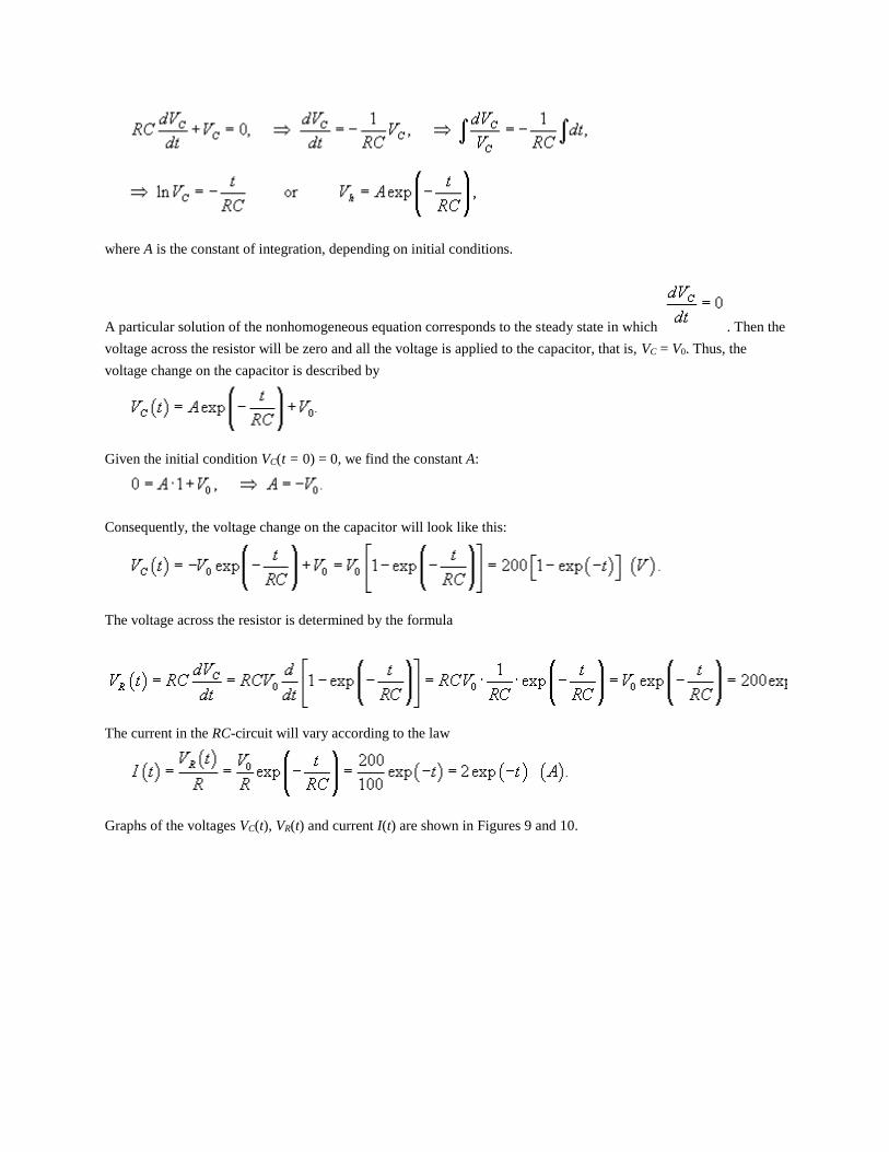
where A is the constant of integration, depending on initial conditions.

A particular solution of the nonhomogeneous equation corresponds to the steady state in which . Then the

voltage across the resistor will be zero and all the voltage is applied to the capacitor, that is, VC = V0. Thus, the

voltage change on the capacitor is described by

Given the initial condition VC(t = 0) = 0, we find the constant A:

Consequently, the voltage change on the capacitor will look like this:

The voltage across the resistor is determined by the formula

The current in the RC-circuit will vary according to the law

Graphs of the voltages VC(t), VR(t) and current I(t) are shown in Figures 9 and 10.

Fig.9

Fig.10

Example 3

An electrical circuit consists of a series-connected resistor R = 1 ohm, a coil with inductance L = 0.25 H and a

capacitor Ñ = 1 µF. How many oscillations will it make before the amplitude of the current is reduced by a factor of

e?

Solution.

In this circuit, damped oscillations will occur with a frequency

The amplitude of the oscillations will decrease according to the law

Suppose that N complete oscillations occurred for time t:

If the amplitude decreased by e times, then one can write the following equation:

Hence we find the number of oscillations N:

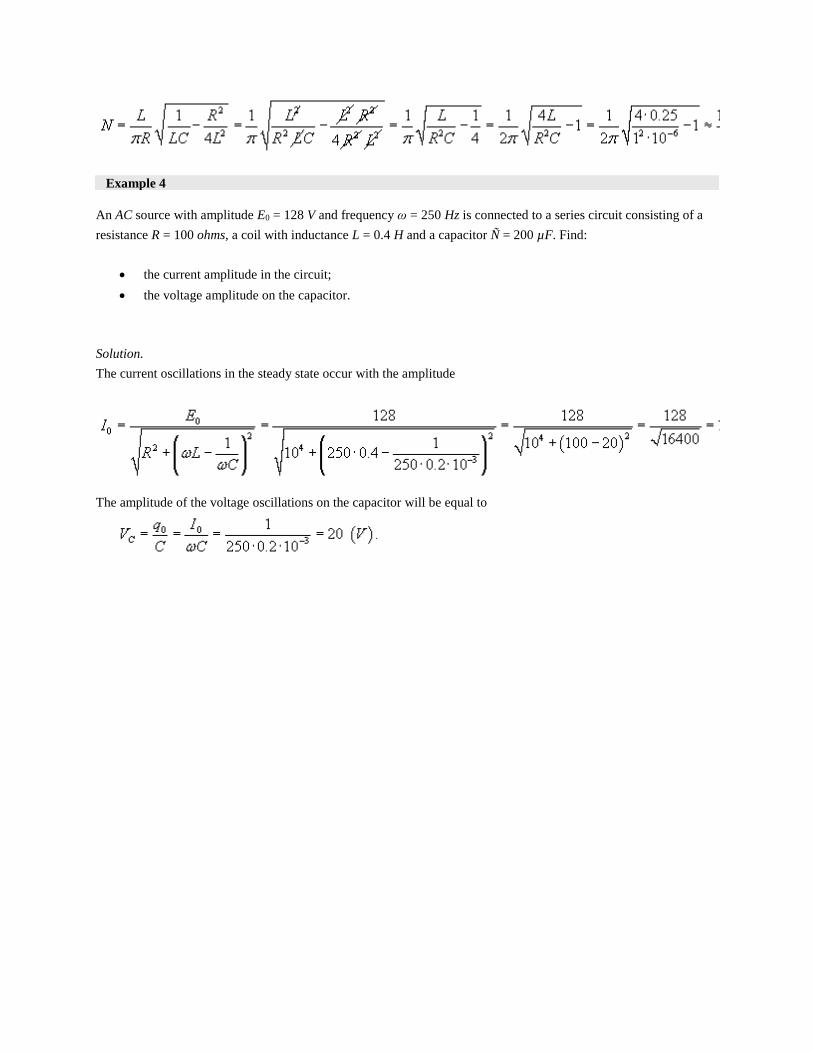
Example 4

An AC source with amplitude E0 = 128 V and frequency ω = 250 Hz is connected to a series circuit consisting of a

resistance R = 100 ohms, a coil with inductance L = 0.4 H and a capacitor Ñ = 200 µF. Find:

the current amplitude in the circuit;

the voltage amplitude on the capacitor.

Solution.

The current oscillations in the steady state occur with the amplitude

The amplitude of the voltage oscillations on the capacitor will be equal to