Crisis of the Chaotic Attractor of a Climate Model: A Transfer Operator Approach · 2015-07-09 ·...

Crisis of the Chaotic Attractor of a Climate Model:

A Transfer Operator Approach

Alexis Tantet

Institute of Marine and Atmospheric research Utrecht, Department of Physics and

Astronomy, University of Utrecht, Utrecht, The Netherlands

E-mail: [email protected]

Valerio Lucarini1,2

1Meteorological Institute and Centre for Earth System Research and Sustainability

(CEN), University of Hamburg, Hamburg, Germany2Department of Mathematics and Statistics, University of Reading, Reading, UK

Frank Lunkeit

Meteorological Institute and Centre for Earth System Research and Sustainability

(CEN), University of Hamburg, Hamburg, Germany

Henk A. Dijkstra

Institute of Marine and Atmospheric research Utrecht, Department of Physics and

Astronomy, University of Utrecht, Utrecht, The Netherlands

Abstract.

The destruction of a chaotic attractor leading to a rough change in the dynamics

of a system as a control parameter is smoothly varied is studied. While bifurcations

involving non-chaotic invariant sets, such as fixed points or periodic orbits, can be

characterised by a Lyapunov exponent crossing the imaginary axis, little is known

about the changes in the Lyapunov spectrum of chaotic attractors during a crisis,

notably because chaotic invariant sets have positive Lyapunov exponents and because

the Lyapunov spectrum varies on the invariant set. However, one would expect the

critical slowing down of trajectories observed at the approach of a classical bifurcation

to persist in the case of a chaotic attractor crisis. The reason is that, as the system

becomes susceptible to the physical instability mechanism responsible for the crisis, it

turns out to be less and less resilient to exogenous perturbations and to spontaneous

fluctuations due to other types of instabilities on the attractor.

The statistical physics framework, extended to nonequilibrium systems, is

particularly well suited for the study of global properties of chaotic systems. In

particular, the semigroup of transfer operators governing the finite time evolution

of probability distributions in phase space and its spectrum characterises both the

relaxation rate of distributions to a statistical steady-state and the stability of this

steady-state to perturbations. If critical slowing down indeed occurs in the approach

to an attractor crisis, the gap in the spectrum (between the leading eigenvalue and the

secondary ones) of the semigroup of transfer operators is expected to shrink.

arX

iv:1

507.

0222

8v1

[nl

in.C

D]

8 J

ul 2

015

Crisis of the Chaotic Attractor of a Climate Model: A Transfer Operator Approach 2

Here we use a high-dimensional, chaotic climate model system in which a transition

from today’s warm climate state to a snow-covered state occurs. This transition is

associated with the destruction of a chaotic attractor as the solar constant is decreased.

We show that critical slowing down develops in this model before the destruction of

the chaotic attractor and that it can be observed from trajectories along the attractor.

In addition, we demonstrate that the critical slowing down can be traced back to the

shrinkage of the leading eigenvalues of coarse-grained approximations of the transfer

operators, constructed from a long simulation of the model system, and that these

eigenvalues capture the fundamental features of the attractor crisis.

Keywords: Attractor Crisis, Transfer Operators, Bifurcation Theory, Response Theory,Structural StabilitySubmitted to: Nonlinearity

1. Introduction

Much progress has been achieved during the last decades regarding bifurcation theory

of low-dimensional dynamical systems and the emergence of aperiodic behaviour and

sensitive dependence to initial conditions, or chaos, when a parameter of the system is

changed. Examples include changes in the Rayleigh number in hydrodynamics [1] or in

the solar constant in climate science [2]. Much less is known, however, on the sudden

appearance or destruction of chaotic attractors. The review by [3] provides a good

starting point regarding the topological description of attractor crisis and the statistics

of chaotic transients. However, little is known regarding the changes in statistical

properties of high-dimensional chaotic systems undergoing an attractor crisis.

While it is a classical result that bifurcations involving non-chaotic invariant sets are

associated with Lyapunov exponents crossing the imaginary axis and with the critical

slowing down of trajectories [4], what happens before a chaotic attractor is destroyed is

less understood. One reason for this is that the Lyapunov spectrum of high-dimensional

systems is virtually inaccessible, either analytically or numerically, even when averaged

over the attractor. However, one would still expect critical slowing down to occur before

the destruction of a chaotic attractor when the control parameter approaches its critical

value at which the crisis occurs.. The system must take more and more time to recover

from exogenous perturbations and also from spontaneous fluctuations due to instabilities

on the attractor. To make the distinction clear between the low-dimensional case and the

chaotic case, we will here prefer the term “attractor crisis” rather than ”bifurcation”.

We will also avoid the term “tipping point”, often used in geophysics, because, even

though a clear definition has been given in [5], its mathematical characterisation remains

vague and may refer to different concepts such as bifurcation, phase transition [6] or

catastrophe [7].


For high-dimensional chaotic systems, geometrical approaches soon become

intractable. However, statistical physics methods developed for nonequilibrium systems

can become very fruitful [8, 9, 10]. Following the ground-breaking ideas of Boltzmann,

a steady-state is described as a time invariant probability measure (a statistical

steady-state) rather than a point in phase space. It is a fundamental property of

nonequilibrium systems that the invariant measure is supported on a strange attractor

with dimensionality lower than that of the phase space. This is the result of a contraction

rate of the phase space that is positive on average and indicates the presence of a positive

rate of entropy production [11, 10]. While most results concerning nonequilibrium

mechanics have been found for the particular case of smooth uniformly hyperbolic

systems [12], their applicability to more general physical systems with a large number of

degrees of freedom and exhibiting chaotic dynamics has been motivated by the Chaotic

Hypothesis in [13] (see also [10]).

In the particular, yet physically highly relevant, case of mixing systems, probability

distributions converge to a unique invariant measure [14]. How such relaxation occurs is

described by the spectrum of transfer operators governing the evolution of distributions

by the dynamics [15, 16, 17]. If a system close to undergo a crisis experiences a slowing

down, the relaxation time of densities to the invariant measure must become very long,

because trajectories take more and more time to converge to the more and more weakly

attracting invariant set. Since this relaxation time can be traced back to the inverse of

the real part of the eigenspectrum of the transfer operators, the latter must thus get

closer and closer to the imaginary axis as the crisis is approached. This simple idea is

also supported by the fact that the gap between the leading eigenvalue of the transfer

operators (associated with the invariant measure) and the secondary eigenvalues gives

a measure of the size of the perturbation for which one can expect the response of the

system to be smooth [18, 19, 20]. Since the response of a system at the crisis is definitely

rough as an infinitesimal perturbation can lead to an attractor change, the gap in the

eigenspectrum of the transfer operators is expected to shrink at the crisis.

For some smooth uniformly hyperbolic systems, the discrete spectrum of the

semigroup of transfer operators acting on Banach spaces, taking into account the

dynamics of contraction and expansion on the stable and unstable manifolds, has been

shown to be stable to perturbations [21, 18] and is accessible via numerical schemes [22].

Moreover, for high-dimensional systems, it has been shown in [23] that the leading part

of the spectrum can also be estimated numerically, but is dependent on the appropriate

choice of an observable [24].

In this study, we explore the properties of an attractor crisis by taking an example

from climate physics. This field has motivated many new concepts in dynamical systems

theory and statistical mechanics. Prominent examples are the case of chaos itself [1],

the use of stochastic dynamical systems [25, 2], the interpretation of complex climatic

features using bifurcation theory [26, 27], the study of predictability of chaotic flows with

its practical implications [28], methods for studying multiscale systems and developing

parameterisations [29, 30, 31, 32], and the use of response theory for studying how the


climate responds to forcing [33, 34, 35, 36, 37].

There are many indications that the climate of our planet is multistable, i.e. the

present astronomical conditions are compatible with two climatic regimes, the present-

day state, and the so-called Snowball state, whereby the Earth experiences extremely

cold conditions. Paleoclimatological studies support the fact that in the distant past

(about 700 Mya) the Earth was in such a Snowball state, and it is still a matter of debate

which mechanisms brought the planet in the present warm state. Note that the issue of

multistability is extremely relevant for the present ongoing investigations of habitability

of exoplanets [38]. Multistability is found for climate models across a hierarchical ladder

of complexity, ranging from simple Energy Balance Models [39, 40, 41] to fully coupled

global circulation models [42, 43]. The robustness of such features is tied to the presence

of an extremely powerful positive feedback which controls the transitions between the

two competing states, the so-called ice-albedo feedback. The presence of a positive

anomaly in ice cover favours a decrease of the absorbed radiation, because ice effectively

reflects incoming solar radiation. This leads to a decrease in the surface temperature,

which favours the formation of ice.

The Planet Simulator (PlaSim) [44, 45] is a model displaying chaotic behavior.

The model is complex enough to represent the main physical mechanisms of climate

multistability, yet sufficiently fast to perform extensive numerical simulations [46, 47].

In the present study, we demonstrate that critical slowing down is observed in PlaSim

before the destruction of the chaotic attractor corresponding to a warm climate.

This slowing down is visible for observables supported by the attractor (thus from

simulations which have already converged to the attractor, without having to perturb

the system). The slowing down is described by the leading eigenvalues of coarse-grained

approximations of the transfer operators, constructed from a long simulation of the

dynamical system and capturing the fundamental features of the attractor crisis.

Section 2 below briefly describes the climate model as well as the set up of different

simulations for varying values of the control parameter. The spectral theory of transfer

operators and the link to the slow decay of correlations associated with critical slowing

down is described in section 3. This section contains also a presentation of the numerical

method used to approximate the spectrum of transfer operators. The results are

presented in section 4, where critical slowing down is shown to occur in the model as

the attractor crisis is approached and to be associated with the approximated leading

eigenvalues of the transfer operators getting closer to the imaginary axis. The results

are summarised in section 5 where we explain the observed critical slowing down from

the theory of boundary crisis [3] and discuss its applications to response theory and the

design of early-warning indicators of the crisis.

2. Model and simulations

As mentioned above, the attractor crises corresponding to the transition between warm

states and snowball climate states has been replicated with qualitatively similar feature


in a variety of models of various degrees of complexity. Given the goals of this study, we

need a climate model that is simple enough to allow for an exploration of parameters in

the vicinity of the attractor crisis and complex enough to feature essential characteristics

of high-dimensional, dissipative, and chaotic systems, as the existence of a limited

horizon of predictability due to the presence of instabilities in the flow. We have opted

for using PlaSim, a climate model of so-called intermediate complexity. This model

has already been used for several theoretical climate studies and provides an efficient

platform for investigating climate transitions when changing boundary conditions and

parameters.

2.1. The Planet Simulator (PlaSim)

The dynamical core of PlaSim is based on the Portable University Model of the

Atmosphere PUMA [48]. The atmospheric dynamics is modelled using the primitive

equations formulated for vorticity, divergence, temperature and the logarithm of surface

pressure. Moisture is included by transport of water vapour (specific humidity). The

governing equations are solved using the spectral transform method [49, 50]. In the

vertical, non-equally spaced sigma (pressure divided by surface pressure) levels are

used. The parametrization of unresolved processes consists of long- [51] and short-

[52] wave radiation, interactive clouds [53, 54, 55], moist [56, 57] and dry convection,

large-scale precipitation, boundary layer fluxes of latent and sensible heat and vertical

and horizontal diffusion [58, 59, 60, 61]. The land surface scheme uses five diffusive

layers for the temperature and a bucket model for the soil hydrology. The oceanic part

is a 50 m mixed-layer (swamp) ocean, which includes a thermodynamic sea ice model

[62].

The horizontal transport of heat in the ocean can either be prescribed or

parametrized by horizontal diffusion. In this case, we consider the simplified setting

where the ocean gives no contribution to the large-scale heat transport. While such

a simplified setting is somewhat less realistic, the climate simulated by the model is

definitely Earth-like, featuring qualitatively correct large scale features and turbulent

atmospheric dynamics. Beside standard output, PlaSim provides comprehensive

diagnostics for the nonequilibrium thermodynamical properties of the climate system

and in particular for local and global energy and entropy budgets. PlaSim is freely

available including a graphical user interface facilitating its use. PUMA and PlaSim

have been applied to a variety of problems in climate response theory [37], entropy

production [63, 64], and in the dynamics of exoplanets [38].

2.2. Attractor crisis and instability mechanism

In [46] and [47], a parameter sweep in PlaSim is performed by changing the solar

constant. The resulting changes in the Global Mean Surface Temperature (GMST)

are represented in figure 1, taken from [47]. For a large range of values of the solar

constant there are two distinct statistical steady states, which can be characterised by


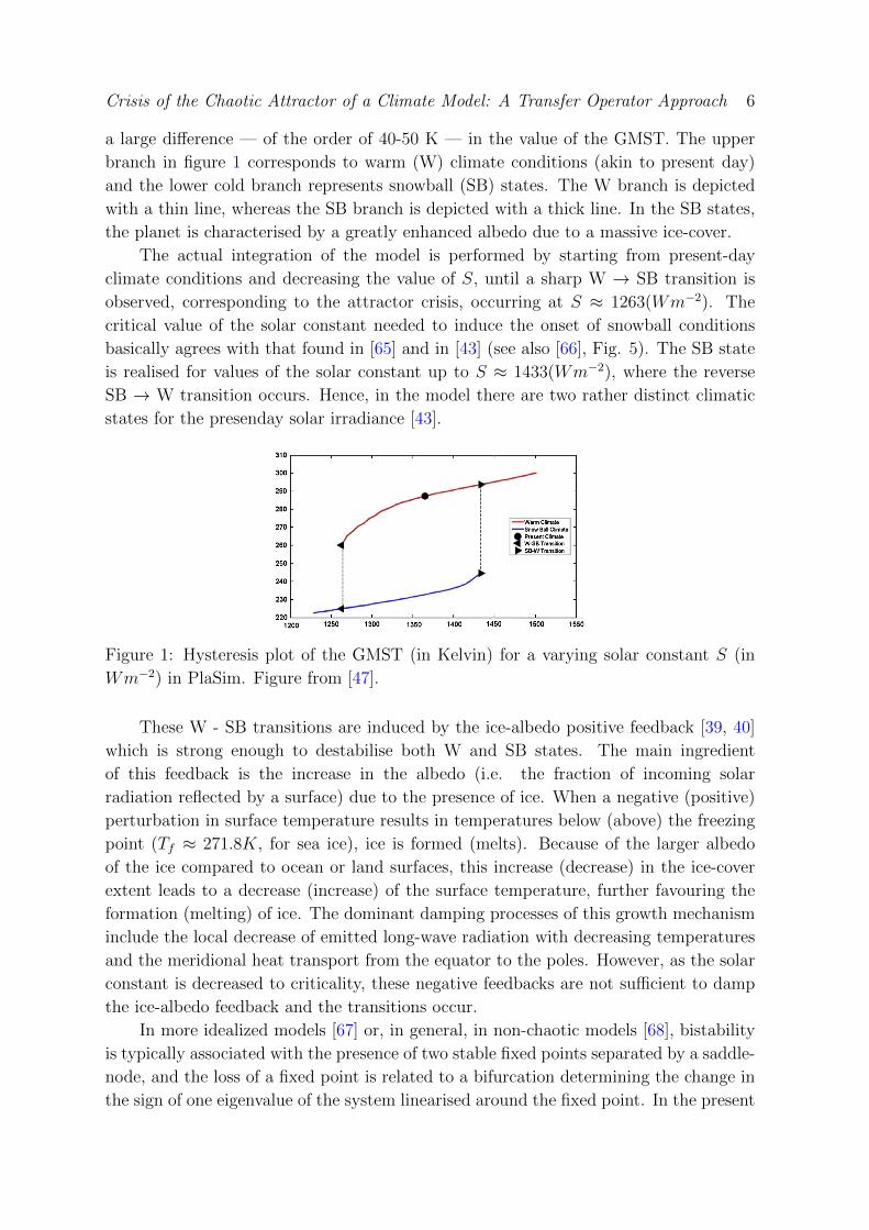
a large difference — of the order of 40-50 K — in the value of the GMST. The upper

branch in figure 1 corresponds to warm (W) climate conditions (akin to present day)

and the lower cold branch represents snowball (SB) states. The W branch is depicted

with a thin line, whereas the SB branch is depicted with a thick line. In the SB states,

the planet is characterised by a greatly enhanced albedo due to a massive ice-cover.

The actual integration of the model is performed by starting from present-day

climate conditions and decreasing the value of S, until a sharp W → SB transition is

observed, corresponding to the attractor crisis, occurring at S ≈ 1263(Wm−2). The

critical value of the solar constant needed to induce the onset of snowball conditions

basically agrees with that found in [65] and in [43] (see also [66], Fig. 5). The SB state

is realised for values of the solar constant up to S ≈ 1433(Wm−2), where the reverse

SB → W transition occurs. Hence, in the model there are two rather distinct climatic

states for the presenday solar irradiance [43].

Figure 1: Hysteresis plot of the GMST (in Kelvin) for a varying solar constant S (in

Wm−2) in PlaSim. Figure from [47].

These W - SB transitions are induced by the ice-albedo positive feedback [39, 40]

which is strong enough to destabilise both W and SB states. The main ingredient

of this feedback is the increase in the albedo (i.e. the fraction of incoming solar

radiation reflected by a surface) due to the presence of ice. When a negative (positive)

perturbation in surface temperature results in temperatures below (above) the freezing

point (Tf ≈ 271.8K, for sea ice), ice is formed (melts). Because of the larger albedo

of the ice compared to ocean or land surfaces, this increase (decrease) in the ice-cover

extent leads to a decrease (increase) of the surface temperature, further favouring the

formation (melting) of ice. The dominant damping processes of this growth mechanism

include the local decrease of emitted long-wave radiation with decreasing temperatures

and the meridional heat transport from the equator to the poles. However, as the solar

constant is decreased to criticality, these negative feedbacks are not sufficient to damp

the ice-albedo feedback and the transitions occur.

In more idealized models [67] or, in general, in non-chaotic models [68], bistability

is typically associated with the presence of two stable fixed points separated by a saddle-

node, and the loss of a fixed point is related to a bifurcation determining the change in

the sign of one eigenvalue of the system linearised around the fixed point. In the present


case, instead, the two branches define the presence of two parametrically modulated (by

the changes in the value of the solar constant) families of disjoint strange attractors, as in

each climate state the dynamics of the system is definitely chaotic. This is suggested by

the fact that, for example, the system features variability on all time-scales [69] which

corresponds, to having intransitive climate conditions [70, 71]. The loss of stability

occurring through the W → SB and SB → W transitions is related to the catastrophic

disappearance of one of the two strange attractors [3]. Near the transitions, the system

features quasi-transitive climate conditions, where long transients can be observed.

2.3. Set-up of long simulations for varying solar constant

While the studies in [46, 47] were focused on the thermodynamic properties of the model

solutions along the two branches of statistical steady-state, we here focus on the changes

in the characteristic evolution of statistics (cf. section 3.1) along the warm branch as

the solar constant S is decreased to its critical value Sc = 1263(Wm−2). The method

presented in section 3.2 requires very long time series of observables. The model is

hence ran for 10,000 years in the configuration presented section 2.1 and for 12 different

fixed values of the solar constant, ranging from the critical value Sc to 1360 (Wm−2)

(approximately the present day value).

The initial state of each simulation is taken in the basin of attraction of the warm

state. While this is difficult to guarantee, taking as initial state the annual mean of the

100th year of a simulation for a solar constant as high as 1450 (Wm−2) (i.e for which

only the warm state exists) resulted in the convergence to the warm state for each of

the 14 values of S. A spin-up of 200 years was more than enough for the simulations

to converge to the statistical steady-state (facilitated by the fact that the ocean has no

dynamics). Preparing for the analysis of section 4, this spin-up period was removed from

the time series. The time series for each observable is subsequently sub-sampled from

daily to annual averages, in order to focus on interannual-to-multidecadal variability

and to avoid having to deal with the seasonal cycle.

3. Transfer operators and their approximation

In this section, we shortly review (i) the connection between the spectrum of the

transfer operator and correlations and (ii) the computational approach to determine

approximations of this spectrum.

3.1. Spectrum of the semigroup of transfer operators and decay of correlations

We consider a dissipative dynamical system (DDS) governed by the system of ODEs

dx(t)

dt= F (x(t)), x ∈ X, (1)

x(0) = x0,


where X = Rd is the phase space and F : X → X is a smooth vector field with flow

{Φτ}τ≥0.Instead of focussing on individual trajectories, one can also follow the evolution

of probability distributions over which observables can be averaged. This is what is

done, for instance, when meteorologists or climate scientists run an ensemble simulation

for which the members differ only in their slightly different initial conditions. As time

evolves, the ensemble spreads more and more over the phase space (i.e. mixes) until

each member becomes decorrelated from the others and averages taken over the ensemble

converge to a constant value. From the conservation of probabilities in phase space, the

evolution of a distribution f by the flow is governed by the Liouville equation:

∂f(x, t)

∂t= Af(x, t), f(x, 0) = f0(x), (2)

with Af = −∇ · (fF ).

The infinitesimal (linear) operator A generates a one-parameter semigroup [72] of

transfer operators {Lτ}τ≥0 yielding the evolution of initial distributions after a finite

time τ . Formally, taking an observable g in a smooth space D and a distribution f in

the dual space D′, the semigroup of transfer operators can be defined, by duality, as

such

〈Lτf(x), g(x)〉 = 〈f(x), g(Φτ (x))〉 , (3)

where 〈f, g〉 is the action of the linear functional f on the smooth test function g,

depending on their functional spaces. In particular, taking f and g in (3) in spaces of

integrable functions, such as L1µ(X) and L∞µ (X), respectively, provides the definition of

the correlation function [14]

Cf,g(τ) =

∫X

f(x)g(Φτ (x))dµ−∫X

fdµ

∫X

gdµ, (4)

where the product of the averages of f and g is determined w.r.t to the measure µ.

The first term in (4) can also be understood as the average of g, as time evolves, with

respect to an initial density f . For mixing systems, as illustrated with the example of the

ensemble simulation above, with unique invariant measure µ, the correlation function

converges to 0 with time. This means that Lτf converges weakly to µ [14].

Of particular interest is the spectrum of the generator A, which we refer to as the

spectrum of the semigroup of transfer operators in the following. Because this operator

is infinite dimensional, its spectrum depends on the functional spaces chosen and may

not only contain discrete eigenvalues, but also a continuous part. In this study, we focus

on dissipative systems (for which the phase space contracts on average, indicative of

positive entropy production, which can result in the fractal structure of the attractor,

see [8, 4]) and the relevant eigenvectors are in spaces of distributions (in the Schwartz

sense). In particular, for mixing systems, the first eigenvalue is simple and equal to 0 and

its eigenvector is the invariant physical measure or statistical steady-state (meaning that

the time average of smooth observables converges to their average w.r.t. the invariant


measure, for an initial set of positive Lebesgue measure), while the rest of the spectrum

is to the left of the imaginary axis.

It has been shown in [18] that, for Anosov flows, there exists a strip γ < <(λ) ≤ 0

in the complex plane, in which only discrete eigenvalues λi of finite multiplicity are to

be found. In the following, we will assume that this is the case, again supported by the

chaotic hypothesis [13, 10]. We furthermore assume, for convenience, that the discrete

spectrum is composed of n simple eigenvalues {λi}1≤i≤n. The spectral decomposition of

the generator then gives for the correlation function

Cf,g(τ) =n∑i=1

eλiτ 〈f, ψ∗i 〉〈ψi, g〉+ 〈Pτf, g〉 −∫X

fdµ

∫X

gdµ, (5)

where ψi and ψ∗i are the eigenvectors of the generator and its adjoint, respectively,

associated with the eigenvalue λi and 〈Pτf, g〉 is the spectral projection of f on the

continuous part of the spectrum applied to g [73]. Note also that, from the Spectral

Mapping Theorem for strongly continuous semigroups (SMT, see [72, chap. IV.3]), eλit

is equal to the eigenvalue ζi(τ) of the transfer operator Lτ (with same eigenvector ψiand adjoint eigenvector ψ∗i ).

The first term in the sum of (5) is associated with the eigenvalue 0, which is unique

for mixing systems, and cancels out with the product of the averages∫Xfdµ

∫Xgdµ.

Furthermore, since the {λi}2≤i≤n have negative real parts, the contribution of each

secondary eigenvalue in the decomposition decays exponentially fast. Eigenvalues closer

to the imaginary axis are, however, responsible for a slower decay, resulting in bumps

in the correlation spectrum (i.e. the Fourier transform of the correlation function)

at a frequency given by the imaginary part of the eigenvalue. The amplitude of the

bumps depend on how f and g project on the eigenvectors ψ∗i and ψi, respectively

[23]. From these considerations, one would expect the spectrum of the semigroup of

transfer operators of a system undergoing a critical slowing down (i.e. a slow decay of

correlations) to accumulate at the imaginary axis. This has indeed been shown to be

the case for the normal forms of the pitchfork and Hopf bifurcations [74, 75] and we will

investigate this here for a chaotic attractor crisis.

3.2. Approximation of the spectrum of the semigroup of transfer operators

As mentioned in the introduction, it has been shown that the discrete spectrum of

transfer operators (of smooth uniformly hyperbolic systems) acting on Banach spaces

is stable to perturbations [21, 18]. These stability results justify the use of numerical

schemes [22] such as Ulam’s method to approximate transfer operators by transition

matrices acting on a discrete space such as a grid spanned by characteristic functions.

Each element of these matrices is a transition probability from one grid-box to the other,

which can be estimated from simulations [76]. Such method has successfully been applied

to low-dimensional systems such as Chua’s ciruit [77] or the Lorenz system [78]. For

high-dimensional systems, however, Ulam’s method becomes prohibitive, as the size of

the grid grows exponentially with the dimension (for an equivalent refinement).


To overcome this curse of dimensionality, it has recently been suggested in [23] to

approximate transfer operators by transition matrices on a reduced, low-dimensional

phase space Y defined by an appropriately chosen observable h : X → Y . As for

Galerkin approximations, the reduced phase space is discretised into a grid of boxes

{Bi}1≤i≤m (another type discretisation could also be used) and the elements of the

transition matrix P hτ at a lag τ and for the observable h, are estimated from a long time

series {xk}1≤k≤T of the system by

(P hτ )ij = P(h(xk+τ ) ∈ Bj|h(xk) ∈ Bi) (6)

=#{(h(xk) ∈ Bi) ∧ (h(xk+τ ) ∈ Bj)}

#{h(xk) ∈ Bi}. (7)

The hats in the formula are there to remind that the (P hτ )ij’s are only likelihood

estimators of the true transition probabilities (P hτ )ij.

Note that because of the high-dimensionality, it is not possible to estimate the

transition probabilities from many simulations starting from different initial conditions

seeding the phase space. Instead, taking advantage of the ergodicity of the invariant

measure implied by the mixing property, only one long simulation is used which, after

an initial spin-up, evolves arbitrarily close to the attractor (in fact, several simulations

starting from a different initial state could also be used, facilitating the numerical

implementation of the method). Thus, unless, for instance, some noise is added to

perturb the system away from the attractor, only transitions corresponding to motions

along the attractor will be resolved. This is an important remark as critical slowing down

may well be only visible when the system is pushed away from the statistical steady-

state (for instance, in the case of a stable fixed point or periodic orbit). However, as will

be shown in section 4, critical slowing down can also be detected through spontaneous

fluctuations (due to instabilities) on the chaotic attractor.

Once the transition matrix P hτ has been estimated for an observable h and a lag τ ,

its l leading eigenvalues {ζhi (τ)}1≤i≤l can be calculated. Applying the SMT, the complex

logarithm of these eigenvalues divided by τ is taken to give

<(λhi (τ)

)= log

(∣∣∣ζhi (τ)∣∣∣) /τ (8)

=(λhi (τ)

)= arg

(ζhi (τ)

)/τ, (9)

The {λhi (τ)}1≤i≤l are the leading eigenvalues that the generator would have if P hτ was

the true transfer operator Lτ . These eigenvalues should be independent of the lag τ ,

but because the transition matrices are estimated on a reduced phase space Y , {P hτ }τ≥0

do not constitute a semigroup and transition matrices estimated for different lags can

yield different {λhi (τ)}1≤i≤l, as is stressed by the addition of the argument τ . Indeed,

the projection of the dynamics on a reduced phase space introduces memory effects,

violating the Markov property of the original system (see Mori-Zwanzig formalism in

[79, 80]). The importance of the choice of the lag τ was already pointed out in [24],

where the method has been applied to the study of atmospheric regime transitions. As


a rule of thumb, a shorter lag allows to access to shorter time scales but a longer lag

allows to treat the fast unresolved variables as decorrelated noise.

While the quality of the approximation of the spectrum of the semigroup of transfer

operators by the spectrum of transition matrices depends on the choice of the observable

h, it has been proven in [23] that the transition probabilities between two sets in the

reduced phase space Y correspond exactly to transition probabilities between the pre-

images of these sets in the full phase space X. Thus, it is expected that the leading

eigenvalues of the transfer operators can be approximated by the spectrum of transition

matrices in the reduced phase space as long as the observable h is appropriately chosen

so as to project significantly on the slowest decaying vectors (the eigenvectors associated

with eigenvalues closest to the imaginary axis).

4. Results

The long simulations described in section 2.3 are now used to study the statistical

changes occurring along the warm branch of statistical steady-states as the solar constant

is decreased towards its critical value Sc. Before applying the methods presented in

section 3, it is first of all shown that critical slowing down can be observed before the

crisis. Note that we have discarded all results relative to values of the solar constant

smaller than 1265(Wm−2), because the sea-ice cover (a discontinuous observable)

becomes very sensitive to the spatial resolution of the model close to criticality. This

results in spurious meta-stable states with different number of grid boxes covered by sea

ice.

4.1. Changes in the statistical steady-state

We start by discussing the statistics of a few observables to stress their key role in the

ice-albedo feedback, the instability mechanism responsible for the attractor crisis (see

section 2.2). Based on physical grounds, the following observables will be used:

• the global fraction of Sea Ice Cover (SIC) in the Northern Hemisphere (NH),

• the Mean Surface Temperature (MST) averaged around the Equator (Eq, i.e. from

15◦S to 15◦N),

The SIC is the primary variable involved in the ice-albedo feedback as an ice-covered

ocean has a much bigger albedo than an ice-free ocean. Sea ice forms when the surface

temperature is below the freezing point (Tf ≈ 271.8K) motivating the choice of a

surface temperature indicator. Furthermore, the MST at the equator is an indicator

of the amount of heat stored in the ocean at low-latitudes (indeed, because the ocean

is slab, the temperature of the water column is uniform and proportional to its heat

content) and that can potentially be transported to high latitudes through horizontal

diffusion in the Ocean or, indirectly, through the general circulation of the Atmosphere.


(a)(c)

(e)

(b) (d) (f)

Figure 2: Sample mean (a-b), variance (c-d) and skewness (e-f) of yearly averages of the

NH SIC fraction (top) and the Eq MST in Kelvin (bottom), versus the solar constant

S (Wm−2).

The sample mean (from the long simulations) of these observables are represented

in figure 2(a-b), allowing us to recap the changes in the climate steady-state [46, 47].

As the solar constant is decreased, less thermal Outgoing Longwave Radiation (OLR) is

necessary to balance the Incoming Shortwave Radiation (ISR) from the sun, so that, as

predicted by the Stefan-Boltzmann law of black bodies, the temperature of the Earth

cools down, explaining the decrease in the Eq MST (fig. 2(b)). The cooling of the surface

of the Earth induces an increase of the extent of the sea ice towards low latitudes, further

weakening the amount of absorbed solar radiation and strengthening the cooling. These

changes in the mean of these observables are smooth, almost linear. Only for a value of

the solar constant smaller than 1280(Wm−2) does the increase in NH SIC strengthen.

However, the sample variance (fig. 2(c-d)) and skewness (fig. 2(e-f)) experience

rougher changes with the solar constant. Indeed, the variance of the NH SIC and Eq

MST increases dramatically for S < 1300(W/m2). This increase indicates that the

ice-albedo feedback is less and less damped as the criticality is approached. Thus, an

anomaly in, for instance, the surface temperature can lead to an increase in the SIC

which will be less easily damped by heat transport from a cooler equator. To stress

the relationship between the NH SIC and the Eq MST, their joint Probability Density

Function (PDF, calculated from the first eigenvector of the transition matrices estimated

in the next section 4.3, yielding exactly the same results as binned estimates, see [24]) is

plotted figure 3, for decreasing values of the solar constant. Apart from the changes in

the mean and the increase in the variance (the axis of each panel have the same scaling),


these plots show that while for S = 1300(Wm−2) (panel (a)) the NH SIC and Eq MST

are not correlated and normally distributed, their distribution becomes more and more

tilted and skewed as the solar constant is decreased (panel (b-d)). This increase in

the skewness of the NH SIC and Eq MST is also visible figure 2(e-f) from which one

can verify that positive values of the NH SIC and negative values of the Eq MST are

favoured as the criticality is approached. This asymmetry is in agreement with the fact

that as the ice-albedo feedback is less and less damped, larger excursions of the SIC to

low latitudes and concomitant cooler temperatures are permitted.

(a) (b)

(c) (d)

Figure 3: Joint PDFs of the NH SIC and Eq MST for (a) S = 1300(Wm−2), (b)

S = 1275(Wm−2), (c) S = 1270(Wm−2) and (d) S = 1265(Wm−2), estimated as the

first eigenvector of the transition matrices estimated in section 4.3. The scaling of the

axis is the same for each panel and is taken so as to span -3 to +3 standard deviations

of the NH SIC and the Eq MST for S = 1265(Wm−2).

4.2. Critical slowing down

Section 4.1 revealed the changes in the moments of the steady-state along the warm

branch, which could be linked to the physical mechanism of ice-albedo feedback. We


now show that, consistent with the increase in variance and skewness of the NH SIC and

Eq MST, their decorrelation time also increases. For this purpose, the sample Auto-

Correlation Function (ACF) and Cross-Correlation Function (CCF) of these observables

are calculated from the simulations presented in section 2.3 and shown in figure 4. Note

that, because the NH SIC and Eq MST are mostly anti-correlated, the absolute value

of the CCF between NH SIC and the Eq MST is plotted in figure 4(c).

From the rather piecewise linear dependence of the correlation functions with the

lag, we observe that the decay of the correlation functions is in qualitative agreement

with a sum of exponentials, as formulated in (5). The fact that the correlation functions

in figure 4 show different decay rates depending on the choice of the observables is

indicative that these observables project differently on the eigenvectors of the generator

of the semigroup of transfer operators and its adjoint, predicted by (5). For example,

that the auto-correlation functions for the NH SIC (fig. 4.a) decay more slowly that the

auto-correlation functions for the Eq MST (fig. 4.b) suggests that the NH SIC projects

more strongly on the part of the spectrum of the semigroup of transfer operators close to

the imaginary axis than the Eq MST. Furthermore, no oscillatory behavior is found in

the correlation functions, indicative that the leading rates in the exponentials must be

real. Note also the strong correlations between the NH SIC and the Eq MST figure 4(c),

in agreement with the PDFs of figure 3. Most importantly, the correlation functions

decay more and more slowly as the solar constant is decreased towards its critical value.

Critical slowing down is thus apparent before the attractor crisis in this model, even

when the unperturbed evolution of the system alone is observed (i.e., from time series

converged to the attractor). This result can be explained in physical terms by the fact

that, as the criticality is approached, spontaneous fluctuations, such as a temperature

anomalies caused by instabilities in the atmosphere, are able to trigger the ice-albedo

feedback. Mathematically, the slowing down and the chaotic attractor crisis cannot

simply be understood in terms of a Lyapunov exponent becoming positive, as in [74, 75]

for the normal forms of the pitchfork and Hopf bifurcations. Indeed, estimates in [69]

suggest that the dynamical core of PlaSim possesses many positive Lyapunov exponents.

As will be discussed in section 5, the slowing down can be explained by the approach of

the stable manifold of a repeller colliding with the attractor at the crisis.

4.3. Changes in the spectrum of transfer operators

The theory presented in section 3.1 suggests that the slowing down observed before the

attractor crisis can be explained by the approach of the spectrum of the semigroup of

transfer operators towards the imaginary axis. To test this theory here, we apply the

numerical method presented in section 3.2 and estimate transition matrices from the

time series of the NH SIC and the Eq MST, observables selected for being most sensitive

to the slowing down (cf. fig. 4) and most relevant in terms of ice-albedo feedback (see

section 4.1).

We first consider a one dimensional reduced phase space defined from the NH SIC


(a)

(b)

(c)

Figure 4: (a) ACF of the NH SIC, (b) ACF of the Eq MST and (c) CCF (in absolute

value) of the NH SIC and Eq MST, for different values of the solar constant; note that

the ordinate has a logarithmic scale.

or the Eq MST alone. A grid of 50 boxes spanning the interval [−5σ, 5σ], where σ is

the standard deviations of each observable, is taken. The width of the domain is chosen


so as to avoid boundary effects which tend to result in a spectrum spuriously too far

from the imaginary axis. The choice of the number of boxes is a trade-off between the

resolution of short spatial and temporal scales and the quality in the estimates of the

transition probabilities. A lag of one year was chosen (i.e., at the sampling frequency

of the time series) which should allow us to determine the eigenvalues corresponding to

time scales as short as one year. However, it is shown in Appendix A that our results

are relatively robust to changes in the grid, the lag and to the sample size.

The leading eigenvalues of the transition matrices estimated for different values of

the solar constant are represented in figure 5 for the NH SIC. The first eigenvalue,

represented in red, is always 0 and is associated with the invariant density of the

transition matrix, which is a projection of the actual invariant measure of the system.

The slowest relaxation time in the series of exponentials in (5) is determined by the

real part of the second eigenvalue and is given in the upper-right corner of figure 5.

Finally, the first five secondary eigenvalues are represented in blue to help following

their evolution. The main result here is that, in agreement with the slower decay of

correlations of the NH SIC observed in figure 4(a), the leading secondary eigenvalues

get closer and closer to the imaginary axis, as the solar constant nears its critical value.

Furthermore, that the leading eigenvalues have vanishing imaginary part agrees with

the fact that no periodicity is found in the correlation functions represented figure 4(a).

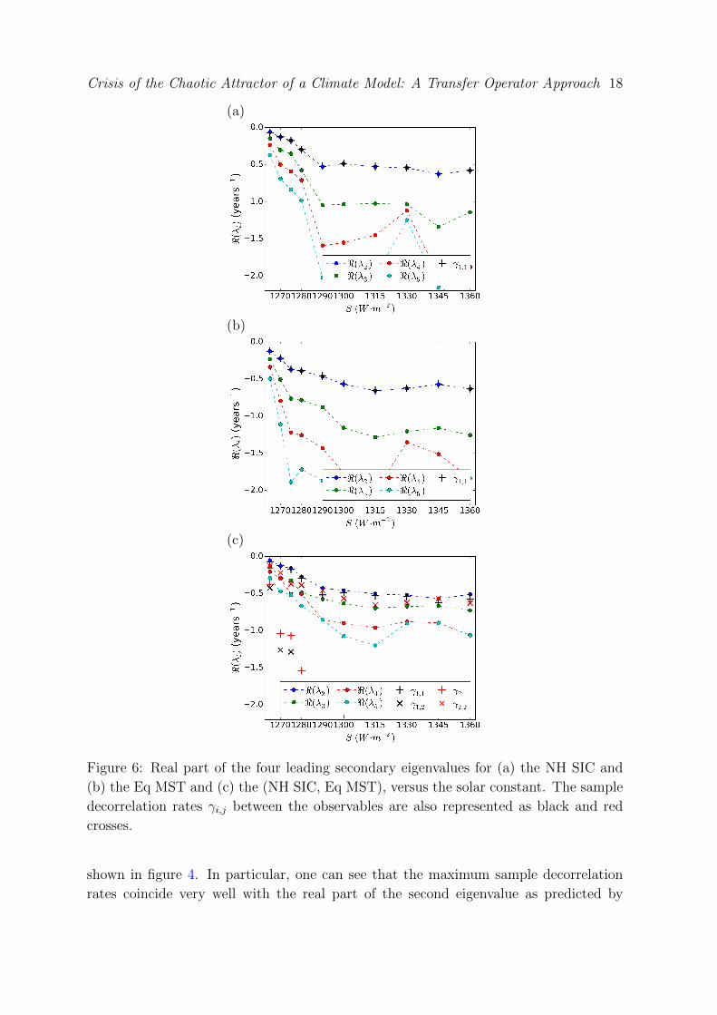
For a more detailed analysis, the real part of the four leading secondary eigenvalues

for the NH SIC and for the Eq MST are plotted figure 6(a) and (b), respectively.

Furthermore, the corresponding plot for the transition matrices estimated using the two

dimensional space composed of both the NH SIC and the Eq MST is also shown in

figure 6(c). For this two dimensional observable, a coarser grid of 25×25 boxes was

used, because of the higher dimension of the reduced phase space compared to the one

dimensional case. In fact, the PDFs represented figure 3 were calculated as the first

left eigenvector of these transition matrices [24]. To these plots are added the sample

decorrelation rates of the observables, calculated from the sample ACFs or CCFs as

γi,j = log(|Cfi,fj(τ)|)/τ , where Cfi,fj(τ) is the sample ACF or CCF with observable fileading observable fj by a lag τ . Here the lag τ was chosen as 1 year, the same as for the

estimation of the transition matrices. For example, γ1,2 in figure 6(c) shows the sample

decorrelation rate with the NH SIC leading the Eq MST by 1 year.

The plots in figure 6 confirm the approach of the imaginary axis by the leading

secondary eigenvalues for the NH SIC, the Eq MST and the (NH SIC, Eq MST), as the

solar constant is decreased to its critical value. In particular, the time scale associated

with the second eigenvalue for the (NH SIC, Eq MST) transition matrices increases

from about 2 years to more than 17 years right before the crisis, yielding a quantitative

measure of the critical slowing down associated with the disappearance of the attractor.

Moreover, for S < 1290(Wm−2), the increase of the real parts is almost linear and is

reminiscent of the results found for bifurcations of low-dimensional systems [74, 75].

Overall, these changes are in agreement with the slower decay of the ACFs and CCFs


(a) (b)

(c) (d)

(e) (f)

Figure 5: Spectra of the transition matrices estimated from the NH SIC for a solar

constant of (a) 1360, (b) 1290, (c) 1280, (d) 1275, (e) 1270 and (f) 1265 (Wm−2).

The first eigenvalue, which is zero, is represented in red, while the first 5 secondary

eigenvalues are represented in blue. The slowest relaxation time in the series of

exponentials in (5) is determined by the real part of the second eigenvalue and is given

in the upper-right corner of the panels.


(a)

(b)

(c)

Figure 6: Real part of the four leading secondary eigenvalues for (a) the NH SIC and

(b) the Eq MST and (c) the (NH SIC, Eq MST), versus the solar constant. The sample

decorrelation rates γi,j between the observables are also represented as black and red

crosses.

shown in figure 4. In particular, one can see that the maximum sample decorrelation

rates coincide very well with the real part of the second eigenvalue as predicted by


(5). This, however, will depend on how well the observables project on the eigenvectors

associated with the second eigenvalue, i.e on how large is the term 〈f, ψ∗2〉〈ψ2, g〉 in (5)

(for instance, if the observable project very strongly on the third eigenvectors compared

to the second, the decorrelation rate may coincide better with the real part of the third

eigenvalue than the second).

5. Summary and Discussion

Motivated by the question whether critical slowing down can be observed in a chaotic

system undergoing an attractor crisis and whether this slowing down can be explained

in terms of spectrum of operators governing the dynamics of statistics, we have taken

as test bed a high-dimensional chaotic climate model undergoing a change of attractor

as a control parameter is varied.

Correlation functions estimated from long simulations of the model have revealed

that a slowing down indeed occurs as the critical value of the control parameter

is approached. Importantly, the slowing down could be seen from the evolution of

observables in steady-state, without having to perturb the system away from the

attractor. This could be explained in physical terms by the fact that the primary

mechanism of instability leading to the destruction of the attractor, the ice-albedo

feedback, is not only activated by exogenous perturbations but also by spontaneous

fluctuations along the attractor (i.e., internal variability, in climatic jargon). This

aspect, related to the presence of positive Lyapunov exponents associated with unstable

processes, makes the treatment of deterministic chaotic systems intrinsically more

interesting than that of simpler systems featuring fixed points or periodic orbits as

attractors.

The topological explanation of this phenomenon is less straightforward, but the

study in [81] suggests that the observed critical slowing down could be related to the

approach of the attractor by a repeller, eventually leading to the crisis. They show

that in a simple, yet physically relevant, energy model able to reproduce accurately the

snowball/snowfree bistability system the attractor crisis is due to the collision of the

attractor of the warm steady-state with a repelling invariant set (the so-called ”edge

state”). Such mechanism has been extensively described in [3] for low-dimensional

systems such as the Henon map or the Lorenz flow and also in [82] for high-dimensional

hydrodynamic flows. In these studies, several attractors coexist for a large range of

parameter values, as in PlaSim, and it is shown that their basins of attraction are

separated by the stable manifold of a repeller, while the closure of the unstable manifold

of the repeller lies on the attractors (the simplest example of this situation would be two

stable fixed points separated by a saddle node). Furthermore, as the control parameter

is varied towards its critical value one of the attractors gets dangerously close to the

stable manifold of the repeller, eventually colliding with it at the crisis. There, one of

the attractors is destroyed and becomes part of the basin of attraction of the other.

Recently the edge state has been constructed also for a simplified climate model


incorporating the dynamical core of PlaSim and a simplified representation of the oceanic

transport and of the ice-albedo feedback [83]. For this case, the above mentioned

mechanism of attractor crisis has been confirmed in detail. We are therefore led to

think that the edge state exists also in the PlaSim configuration adopted here. The

critical slowing down observed at the approach of the crisis could thus be explained by

the influence of the stable manifold of the edge state on the dynamics on the attractor.

Indeed, trajectories along the attractor approaching the region in which the stable

manifold of the edge state is close are expected to spend more and more time in this

region, resulting in an increase of the correlations (and thus of predictability). Note

that understanding the properties of the edge state is key to predicting the features of

the noise induced transitions across the two basins of attractions.

The second step of this study was to verify that the slowing down of the decay

of correlations can be described in terms of spectrum of transfer operators, relying

on approximations by Markov transition matrices acting on a reduced phase space.

Approximating this spectrum for systems with competing time-scales can reveal much

reacher dynamics than by the estimation of the decorrelation rates alone. Of course,

one cannot expect to recover the discrete part of the spectrum of transfer operators

very accurately with such coarse-grained representations. However, with an appropriate

choice of observable one can expect to get good estimates of the leading eigenvalues.

The observable should be such that it projects well on the leading eigenvectors of the

semigroup of transfer operators. However, these eigenvectors are difficult to access

and the choice of the observable should eventually be guided by the behaviour of its

correlation functions and by an understanding of the fundamental physical mechanisms

responsible for the slow dynamics. Moreover, if the reduced phase space on which

the transition matrices are estimated is defined by an observable which is such that its

correlation functions decay slowly, unresolved fluctuations (i.e orthogonal to the reduced

phase space) are more likely to experience a correlation decay faster than the observable

itself and could thus be approximated by a decorrelated noise. In this case, the evolution

of the observable could be modelled by a stochastic process on the reduced phase space

and the evolution of densities in this space would itself be governed by the semigroup

of transfer operators of the stochastic process (see [24] for a detailed discussion).

Contrary to the changes in the statistical moments of observables (cf. section 4.1),

which are expected to vary depending on the topology of the attractor, the approach of

the spectrum of the semigroup of transfer operators to the imaginary axis responsible for

the slowing down as an attractor crisis is approached is expected to be rather general.

It is based on both the physical idea that the instability mechanism becomes more and

more easy to trigger by spontaneous fluctuations along the chaotic attractor and on the

discussion on the collision with an edge state. In fact the narrowing of the spectral gap

between the eigenvalue 0 and the secondary eigenvalues of the semigroup is an indicator

that the radius of convergence of the series expansion of the perturbed invariant measure

shrinks [84, 20]. In other words, the size of the perturbation for which response theory

applies [19] vanishes at the criticality, accordingly to the fact that a dramatic change in


the statistics occurs during the attractor crisis.

Finally, we have seen in section 4.3, that the change in the spectrum of the

semigroup of transfer operators (and, a fortiori, in the decorrelation rates) is very

smooth before the crisis, in agreement with the analytical results in [74, 75] for low-

dimensional systems. Invoking the chaotic hypothesis, such numerical results could be

explained by the differentiability of the spectrum of Anosov systems, proved in [21]

for appropriate Banach spaces. The fact that critical slowing down can be observed

from long time series of a high-dimensional chaotic system suggests that classical early

warning indicators such as the lag-1 autocorrelation [85], could be used to detect a

chaotic attractor crisis from observations. However, the smoothness in the change of

the spectrum of the semigroup of transfer operators suggests that autocorrelation-based

indicators cannot be expected to give a very strong signal at the approach of an attractor

crisis. This analysis thus shows, that even though the methodology presented section

3 is too demanding in terms of data to apply it to observations and use the spectral

gap as an early-warning indicator of a crisis, it is very well suited to understand and

design such indicators in the more general context of high-dimensional chaotic (and also

stochastic) systems than the one of AR(1) processes for which the lag-1 auto-correlation

indicator was originally developed in [85].

Acknowledgments

AT and HD would like to acknowledge the support of the LINC project (no. 289447)

funded by EC’s Marie-Curie ITN program (FP7-PEOPLE-2011-ITN). VL acknowledges

fundings from the Cluster of Excellence for Integrated Climate Science (CLISAP)

and from the European Research Council under the European Communitys Seventh

Framework Programme (FP7/2007-2013)/ERC Grant agreement No. 257106 Starting

Investigator Grant NAMASTE - Thermodynamics of the Climate System.

Appendix A. Robustness of the numerical estimates of the spectrum of the

reduced transition matrices

In this section, we test the robustness of the eigenvalues of the reduced transition

matrices represented figure 6 to the sampling length, the grid size and the lag. For

convenience, all the tests are presented for the NH SIC only. However, the corresponding

tests done for the Eq MST and (NH SIC, Eq MST) do not challenge the conclusions

taken in this study. Unless specified, all the parameters used in the following to estimate

the transition matrices, such as the length of the times series, the grid, or the lag, are

taken the same as for the ones used section 4.3 to produce figure 6.

Appendix A.1. Robustness to the sampling length

To test the robustness of the approximated spectra to the length of the time series used

to estimate the transition probabilities, one could calculate confidence intervals from


a version of the non-parametric bootstrap (see [86, 87]), adapted to the estimation of

transition matrices (see [88]) as was done in [23, 24]. Instead, we simply look at the

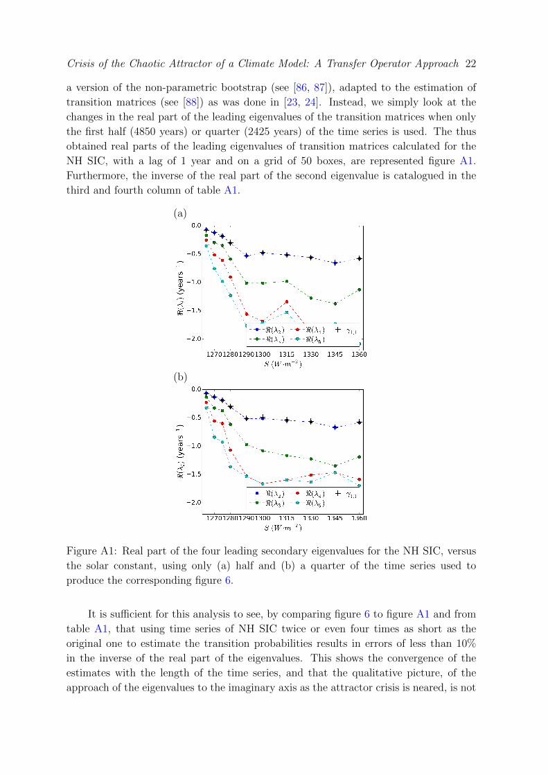
changes in the real part of the leading eigenvalues of the transition matrices when only

the first half (4850 years) or quarter (2425 years) of the time series is used. The thus

obtained real parts of the leading eigenvalues of transition matrices calculated for the

NH SIC, with a lag of 1 year and on a grid of 50 boxes, are represented figure A1.

Furthermore, the inverse of the real part of the second eigenvalue is catalogued in the

third and fourth column of table A1.

(a)

(b)

Figure A1: Real part of the four leading secondary eigenvalues for the NH SIC, versus

the solar constant, using only (a) half and (b) a quarter of the time series used to

produce the corresponding figure 6.

It is sufficient for this analysis to see, by comparing figure 6 to figure A1 and from

table A1, that using time series of NH SIC twice or even four times as short as the

original one to estimate the transition probabilities results in errors of less than 10%

in the inverse of the real part of the eigenvalues. This shows the convergence of the

estimates with the length of the time series, and that the qualitative picture, of the

approach of the eigenvalues to the imaginary axis as the attractor crisis is neared, is not


affected by the sampling length.

Appendix A.2. Robustness to the grid size

The robustness of our results to the size of the grid is now addressed. Figure A2(a) to

(c) represents the real part of the leading eigenvalues of transition matrices estimated

on a grid of 25, 75 or a 100 boxes, respectively, instead of the original grid of 50 boxes

used to produce figure 6. Figure A2(a-c) and figure 6 are qualitatively similar, with

the approach to 0 of the real part of the leading eigenvalues as the solar constant is

decreased. The inverse of the real part of the second eigenvalue is also given in the fifth

to the seventh column of table A1 from which one can see that increasing the resolution

results in differences in the inverse of the real part of the second eigenvalue of less than

5%. This suggests that the grid of 50 boxes used for the NH SIC is sufficiently thin to

obtain good estimates of, at least, the second eigenvalue, allowing one to conclude that

the outcome of this study is not challenged by the coarse resolution of the grid used to

estimate the transition matrices.

Appendix A.3. Robustness to the lag

All the transition matrices in section 4.3 were calculated for a lag of 1 year, in order

to have access to time scales as short as possible. However, due to the fact that the

transition matrices are calculated on a reduced phase space, {P hτ }τ≥0 does not constitute

a semigroup, so that the SMT does not apply and the eigenvalues {λhi (τ)}1≤i≤l depend

on the lag for which the transition matrix has been estimated. To verify that the

conclusions of the analysis presented section 4.3 are not questioned by a different choice

of the lag, we represent, in figure A3(a) and (b), the real part of the leading secondary

eigenvalues, calculated, as for figure 6, for the NH SIC and on a grid of 50 boxes but

for a longer lag of 3 and 5 years, respectively. Again, the inverse of the real part of the

first secondary eigenvalue thus obtained is catalogued in table A1.

It is obvious from figure A3, that eigenvalues far away from the imaginary axis are

not well estimated for long lags as they are cornered to some cut-off value. This effect

is expected, since the lag used to estimate the transition matrices gives a lower bound

to the time scale associated with the eigenvalues that the method presented in section

3.2 can resolve. However, even when a lag of 5 years is taken, the approach of the

second eigenvalue to the imaginary axis as the control parameter is decreased towards

its critical value can still be observed figure A3(b), since the real part of this eigenvalue

corresponds to a time scale larger than 5 years for S < 1280(Wm−2).


(a)

(b)

(c)


the solar constant, using a grid of (a) 25 boxes, (b) 75 boxes and (c) a 100 boxes,

compared to the 50 boxes grid used to produce figure 6.

References

[1] Lorenz E N 1963 Journal of the atmospheric sciences 20 130

[2] Saltzman B 2002 Dynamical paleoclimatology: generalized theory of global climate change (San


(a)

(b)


the solar constant, using a lag of (a) 3 years and (b) 5 years, compared to the lag of 1

year used to produce figure 6.

Diego: Academic Press)

[3] Grebogi C, Ott E and Yorke J a 1983 Physica D: Nonlinear Phenomena 7 181–200

[4] Strogatz S H 1994 Nonlinear Dynamics and Chaos: With Applications to Physics, Biology,

Chemistry, and Engineering (Boulder: Westview Press)

[5] Lenton T M, Held H, Kriegler E, Hall J W, Lucht W, Rahmstorf S and Schellnhuber H J 2008

Proceedings of the National Academy of Sciences of the United States of America 105 1786–93

[6] Le Bellac M, Mortessagne F and Batrouni G G 2004 Equilibrium and Non-Equilibrium Statistical

Thermodynamics (Cambridge University Press)

[7] Arnol’d V 1986 Catastrophe theory (Berlin: Springer-Verlag)

[8] Eckmann J P and Ruelle D 1985 Reviews of modern physics 57 617

[9] Young L S 2002 Journal of Statistical Physics 108 733–754

[10] Gallavotti G and Lucarini V 2014 Equivalence of Non-equilibrium Ensembles and Representation

of Friction in Turbulent Flows: The Lorenz 96 Model vol 156

[11] Ruelle D 1989 Chaotic Evolution and Strange Attractors (Cambridge: Cambridge University Press)

[12] Young L s 1998 Notices of the AMS 45 1318–1328

[13] Gallavotti G and Cohen E G D 1995 Journal of Statistical Physics 80 931–970

[14] Lasota A and Mackey M C 1994 Chaos, Fractals and Noise (Berlin: Springer)

[15] Ruelle D 1986 Physical review letters 56 405–407


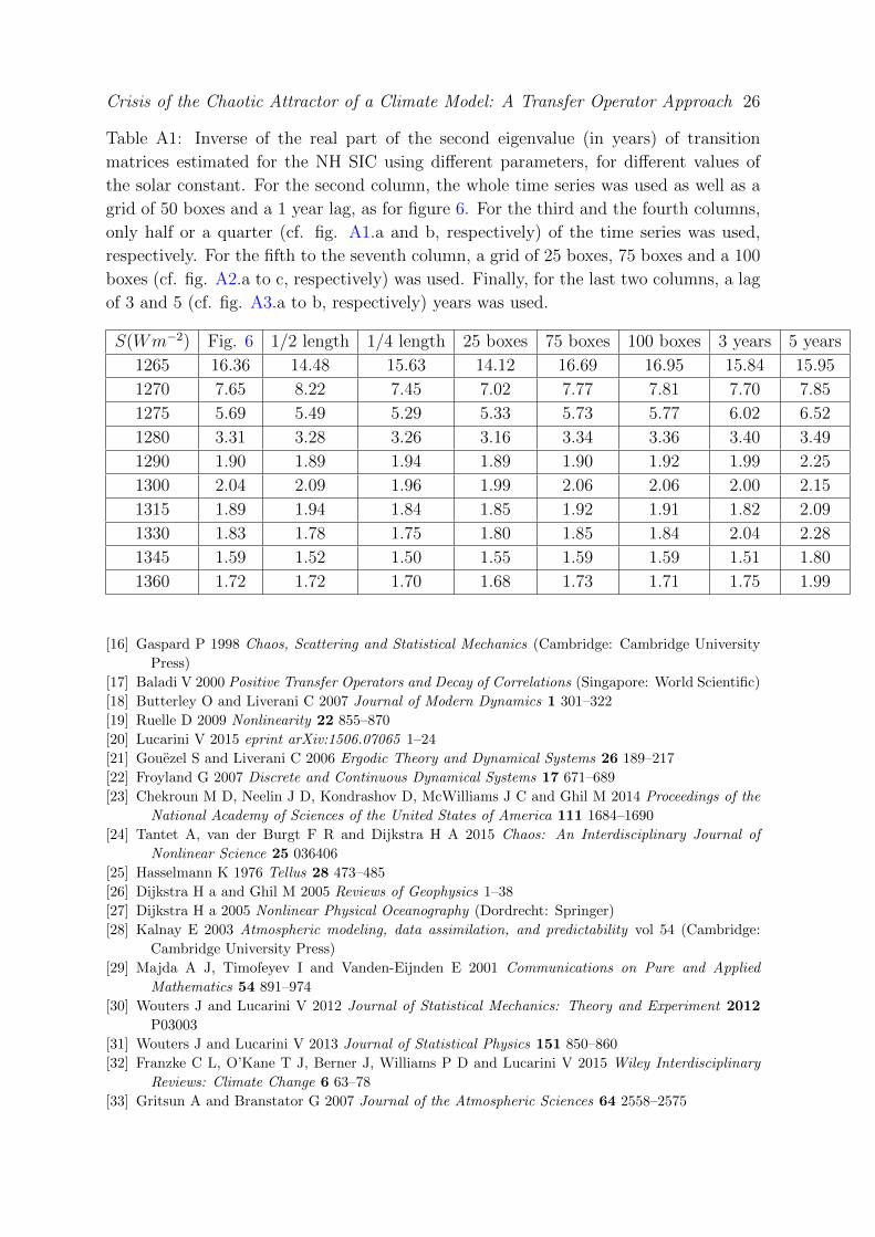
Table A1: Inverse of the real part of the second eigenvalue (in years) of transition

matrices estimated for the NH SIC using different parameters, for different values of

the solar constant. For the second column, the whole time series was used as well as a

grid of 50 boxes and a 1 year lag, as for figure 6. For the third and the fourth columns,

only half or a quarter (cf. fig. A1.a and b, respectively) of the time series was used,

respectively. For the fifth to the seventh column, a grid of 25 boxes, 75 boxes and a 100

boxes (cf. fig. A2.a to c, respectively) was used. Finally, for the last two columns, a lag

of 3 and 5 (cf. fig. A3.a to b, respectively) years was used.

S(Wm−2) Fig. 6 1/2 length 1/4 length 25 boxes 75 boxes 100 boxes 3 years 5 years

1265 16.36 14.48 15.63 14.12 16.69 16.95 15.84 15.95

1270 7.65 8.22 7.45 7.02 7.77 7.81 7.70 7.85

1275 5.69 5.49 5.29 5.33 5.73 5.77 6.02 6.52

1280 3.31 3.28 3.26 3.16 3.34 3.36 3.40 3.49

1290 1.90 1.89 1.94 1.89 1.90 1.92 1.99 2.25

1300 2.04 2.09 1.96 1.99 2.06 2.06 2.00 2.15

1315 1.89 1.94 1.84 1.85 1.92 1.91 1.82 2.09

1330 1.83 1.78 1.75 1.80 1.85 1.84 2.04 2.28

1345 1.59 1.52 1.50 1.55 1.59 1.59 1.51 1.80

1360 1.72 1.72 1.70 1.68 1.73 1.71 1.75 1.99

[16] Gaspard P 1998 Chaos, Scattering and Statistical Mechanics (Cambridge: Cambridge University

Press)

[17] Baladi V 2000 Positive Transfer Operators and Decay of Correlations (Singapore: World Scientific)

[18] Butterley O and Liverani C 2007 Journal of Modern Dynamics 1 301–322

[19] Ruelle D 2009 Nonlinearity 22 855–870

[20] Lucarini V 2015 eprint arXiv:1506.07065 1–24

[21] Gouezel S and Liverani C 2006 Ergodic Theory and Dynamical Systems 26 189–217

[22] Froyland G 2007 Discrete and Continuous Dynamical Systems 17 671–689

[23] Chekroun M D, Neelin J D, Kondrashov D, McWilliams J C and Ghil M 2014 Proceedings of the

National Academy of Sciences of the United States of America 111 1684–1690

[24] Tantet A, van der Burgt F R and Dijkstra H A 2015 Chaos: An Interdisciplinary Journal of

Nonlinear Science 25 036406

[25] Hasselmann K 1976 Tellus 28 473–485

[26] Dijkstra H a and Ghil M 2005 Reviews of Geophysics 1–38

[27] Dijkstra H a 2005 Nonlinear Physical Oceanography (Dordrecht: Springer)

[28] Kalnay E 2003 Atmospheric modeling, data assimilation, and predictability vol 54 (Cambridge:

Cambridge University Press)

[29] Majda A J, Timofeyev I and Vanden-Eijnden E 2001 Communications on Pure and Applied

Mathematics 54 891–974

[30] Wouters J and Lucarini V 2012 Journal of Statistical Mechanics: Theory and Experiment 2012

P03003

[31] Wouters J and Lucarini V 2013 Journal of Statistical Physics 151 850–860

[32] Franzke C L, O’Kane T J, Berner J, Williams P D and Lucarini V 2015 Wiley Interdisciplinary

Reviews: Climate Change 6 63–78

[33] Gritsun A and Branstator G 2007 Journal of the Atmospheric Sciences 64 2558–2575


[34] Abramov R V and Majda A J 2007 Nonlinearity 20 2793–2821

[35] Lucarini V and Sarno S 2011 Nonlinear Processes in Geophysics 18 7–28

[36] Lucarini V, Blender R, Herbert C, Ragone F, Pascale S and Wouters J 2014 Reviews of Geophysics

52 1 – 51

[37] Ragone F, Lucarini V and Lunkeit F 2015 Climate Dynamics 1–25

[38] Lucarini V, Pascale S, Boschi R, Kirk E and Iro N 2013 Astronomische Nachrichten 334 576–588

[39] Budyko M I 1969 Tellus 21 611 – 619

[40] Sellers W D 1968 Journal of Applied Meteorology 8 392–400

[41] Ghil M 1976 Journal of Atmospheric Sciences 33 3–20

[42] Pierrehumbert R, Abbot D, Voigt A and Koll D 2011 Annual Review of Earth and Planetary

Sciences 39 417–460

[43] Voigt A and Marotzke J 2010 Climate Dynamics 35 887–905

[44] Fraedrich K, Jansen H, Kirk E and Lunkeit F 2005 Meteorologische Zeitschrift 14 305–314

[45] Fraedrich K, Jansen H, Kirk E, Luksch U and Lunkeit F 2005 Meteorologische Zeitschrift 14

299–304

[46] Lucarini V, Fraedrich K and Lunkeit F 2010 Quarterly Journal of the Royal Meteorological Society

136 2–11

[47] Boschi R, Lucarini V and Pascale S 2013 Icarus 226 1724–1742

[48] Fraedrich K, Kirk E and Lunkeit F 1998 PUMA: Portable University Model of the Atmosphere

Tech. rep. Deutsches Klimarechenzentrum Hamburg

[49] Eliasen E, Machenhauer B and Rasmussen E 1970 On a numerical method for integration of the

hydrodynamical equations with a spectral representation of the horizontal fields Tech. rep. Inst.

of Theor. Met., Københavns University Copenhagen

[50] Orszag S A 1970 Journal of the Atmospheric Sciences 27 890–895

[51] Sasamori T 1968 Journal of Applied Meteorology 7 721–729

[52] Lacis A a and Hansen J 1974 Journal of the Atmospheric Sciences 31 118–133

[53] Stephens G L, Paltridge G W and Platt C M R 1978 Journal of the Atmospheric Sciences 35

2133–2141

[54] Stephens G L, Ackerman S and Smith E A 1984 Journal of the Atmospheric Sciences 41 687–690

[55] Slingo A and Slingo J M 1991 Journal of Geophysical Research 96 15341

[56] Kuo H L 1965 Journal of the Atmospheric Science 22 40–63

[57] Kuo H L 1974 Journal of the Atmospheric Sciences 31 1232–1240

[58] Louis J F 1979 Boundary-Layer Meteorology 17 187–202

[59] Louis J F, Tiedke M and Geleyn M 1981 A short history of the PBL parameterisation at

ECMWF Proceedings of the ECMWF Workshop on Planetary Boundary Layer Parameterization

(Reading) pp 59–80

[60] Laursen L and Eliasen E 1989 Tellus 41A 385–400

[61] Roeckner E, Arpe K, Bengtsson L, Brinkop S, Dumenil L, Esch M, Kirk E, Lunkeit F, Ponater M,

Rockel B, Sausen R, Schlese U, Schubert S and Windelband M 1992 Simulation of present day

climate with the ECHAM model: impact of model physics and resolution. Technical Report, 93

Tech. rep. Max Planck Institut fur Meteorologie Hamburg

[62] Semtner A J 1976 Journal of Physical Oceanography 6 379–389

[63] Lucarini V and Pascale S 2014 Climate Dynamics 43 981–1000

[64] Fraedrich K and Lunkeit F 2008 Tellus, Series A: Dynamic Meteorology and Oceanography 60

921–931

[65] Poulsen C J and Jacob R L 2004 Paleoceanography 19 1–11

[66] Wetherald R T and Manabe S 1975 Journal of Atmospheric Sciences 32 2044–2059

[67] Scott J R, Marotzke J and Stone P H 1999 Journal of Physical Oceanography 29 351

[68] Lucarini V, Calmanti S and Artale V 2007 Russian Journal of Mathematical Physics 14 224–231

[69] Schalge B, Blender R, Wouters J, Fraedrich K and Lunkeit F 2013 Physical Review E 87 052113

[70] Lorenz E N 1967 The nature and theory of the general circulation of the atmosphere (World


Meteorological Organization)

[71] Peixoto J P and Oort A H 1992 Physics of Climate (American Institute of Physics)

[72] Engel K J and Nagel R 2001 One-parameter semigroups for linear evolution equations (New York:

Springer)

[73] Butterley O 2015 Ergodic Theory and Dynamical Systems 1–13

[74] Gaspard P, Nicolis G, Provata A and Tasaki S 1995 Physical Review E 51 74–94

[75] Gaspard P and Tasaki S 2001 Physical Review E 64 056232

[76] Dellnitz M and Junge O 1999 SIAM Journal on Numerical Analysis 36 491–515

[77] Dellnitz M and Junge O 1997 International Journal of Bifurcation and Chaos 7 2475–2485

[78] Froyland G and Padberg K 2009 Physica D: Nonlinear Phenomena 238 1507–1523

[79] Zwanzig R 2001 Nonequilibrium Statistical Mechanics (Oxford: Oxford University Press)

[80] Chorin A J, Hald O H and Kupferman R 2002 Physica D: Nonlinear Phenomena 166 239–257

[81] Bodai T, Lucarini V, Lunkeit F and Boschi R 2013 preprint arXiv:1402.3269v1

[82] Schneider T M, Eckhardt B and Yorke J a 2007 Physical Review Letters 99 1–4

[83] Lucarini V and Bodai T 2015 Unpublished

[84] Kato T 1995 Perturbation Theory for Linear Operators Perturbation Theory for Linear Operators

(Berlin: Springer)

[85] Held H and Kleinen T 2004 Geophysical Research Letters 31 1–4

[86] Efron B 1980 The Jacknife, the bootstrap, and other resampling plans Tech. rep. Stanford

University Stanford

[87] Mudelsee M 2010 Climate Time Series Analysis: Classical Statistical and Bootstrap Methods

(Dordrecht: Springer)

[88] Craig B a and Sendi P P 2002 Health economics 11 33–42

Crisis of the Chaotic Attractor of a Climate Model: A Transfer Operator Approach · 2015-07-09 ·...

Documents

Transcript of Crisis of the Chaotic Attractor of a Climate Model: A Transfer Operator Approach · 2015-07-09 ·...