F

;., NASA Contractor Report 3790

Creep-Rupture Reliability Analysis

Alonso Peralta-Duran and Paul H. Wirsching

NASA CR 3790 c.1

GRANT NAG341 MARCH 1984

LOAN COPY: RETURN TO AFWL TECHNICAL LiORARY KIRTLAEJD AFB, N.M. 87'117

https://ntrs.nasa.gov/search.jsp?R=19840011857 2018-07-29T21:55:02+00:00Z

TECH LIBRARY KAFB, NM

NASA Contractor Report 3790

Creep-Rupture Reliability Analysis

Alonso Peralta-Duran and Paul H. Wirsching The University of Arizona Tucson, Arizona

Prepared for Lewis Research Center under Grant NAG3-41

National Aeronautics and Space Administration

Scientific and Technical Information Office

1984

iii

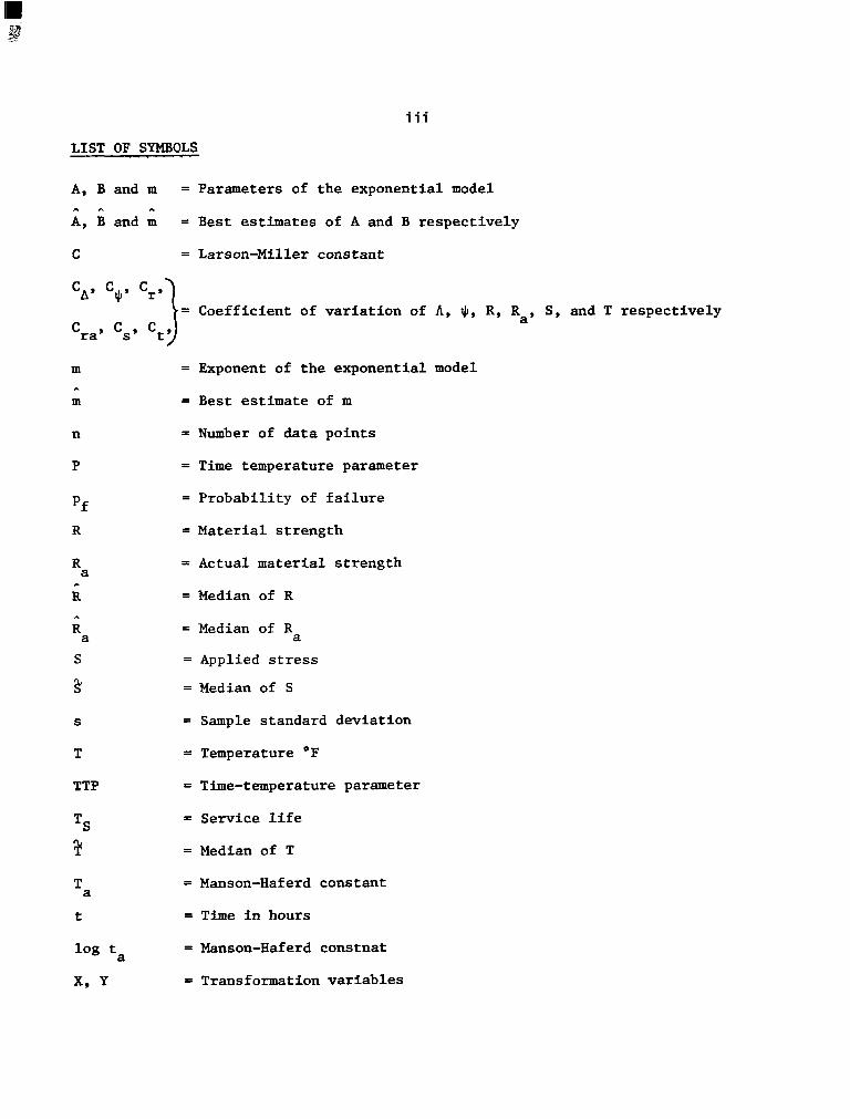
LIST OF SYMBOLS

A, B and m = Parameters of the exponential model

A, B and m = Best estimates of A and B respectively A & A

C = Larson-Miller constant

c*, C$, cr, = Coefficient of variation of A , JI, R, Ra, S, and T respectively

= Exponent of the exponential model

= Best estimate of m

= Number of data points

= Time temperature parameter

= Probability of failure

= Material strength

= Actual material strength

= Median of R

= Median of Ra

= Applied stress

= Median of S

= Sample standard deviation

= Temperature OF

= Time-temperature parameter

= Service life

= Median of T

= Manson-Haferd constant

= Time in hours

= Manson-Haferd constnat

= Transformation variables

i v

LIST OF GREEK SYMBOLS

B = Safety index

@ = Standard normal cdf

A Y = Variables which quantify the bias of the model

A Y = Mean of A and Y respectively

A ‘4 = Median of A and Y respectively

”

% %

% = Mean value (subscript denotes random variable)

Ox = Standard deviation (subscript denotes random variable)

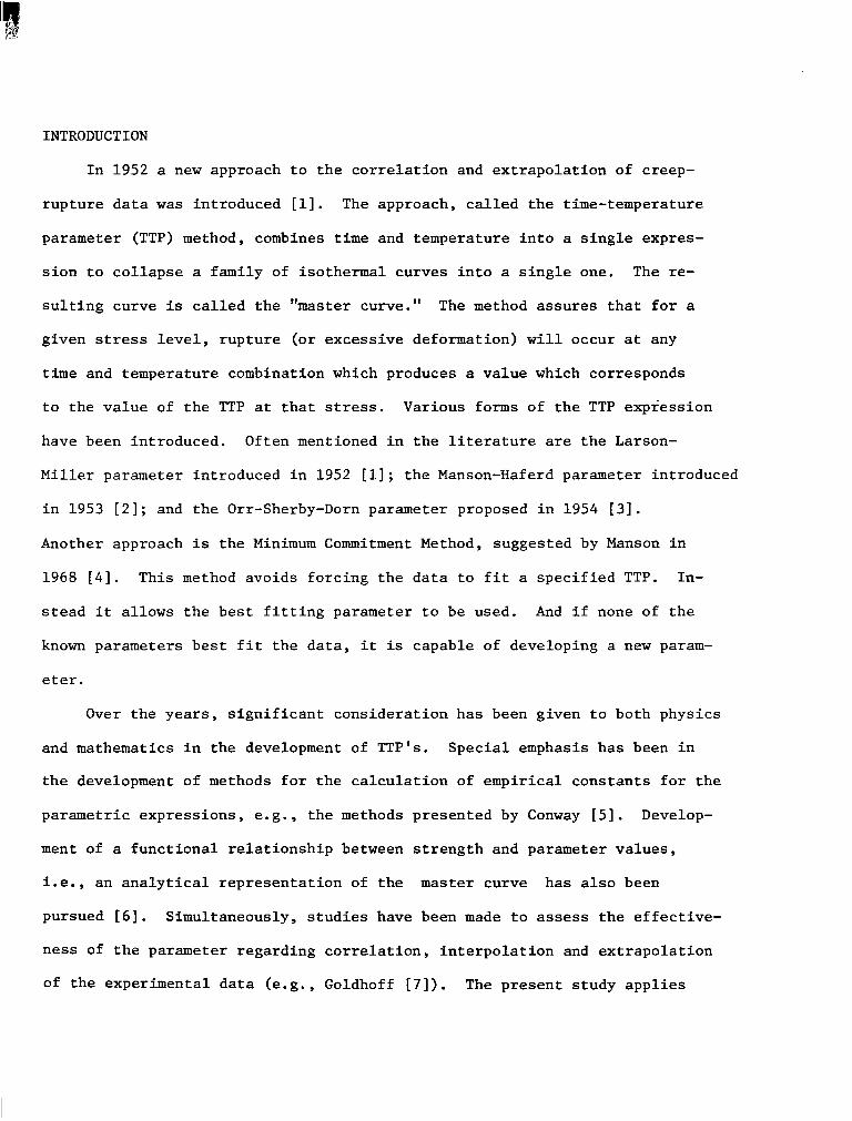
INTRODUCTION

In 1952 a new approach to the correlation and extrapolation of creep-

rupture data was introduced [l]. The approach, called the time-temperature

parameter (TTP) method, combines time and temperature into a single expres-

sion to collapse a family of isothermal curves into a single one. The re-

sulting curve is called the "master curve." The method assures that for a

given stress level, rupture (or excessive deformation) will occur at any

time and temperature combination which produces a value which corresponds

to the value of the TTP at that stress. Various forms of the TTP expression

have been introduced. Often mentioned in the literature are the Larson-

Miller parameter introduced in 1952 [l]; the Manson-Haferd parameter introduced

in 1953 [2]; and the Orr-Sherby-Dorn parameter proposed in 1954 [3].

Another approach is the Minimum Commitment Method, suggested by Manson in

1968 [ 4 ] . This method avoids forcing the data to fit a specified TTP. In-

stead it allows the best fitting parameter to be used. And if none of the

known parameters best fit the data, it is capable of developing a new param-

eter.

Over the years, significant consideration has been given to both physics

and mathematics in the development of TTP's. Special emphasis has been in

the development of methods for the calculation of empirical constants for the

parametric expressions, e.g., the methods presented by Conway [5]. Develop-

ment of a functional relationship between strength and parameter values,

i.e., an analytical representation of the master curve has also been

pursued [ 6 ] . Simultaneously, studies have been made to assess the effective-

ness of the parameter regarding correlation, interpolation and extrapolation

of the experimental data (e.g., Goldhoff [7]). The present study applies

2

probabilistic design theory to creep-rupture data analysis, bringing state

of the art methods to the design of components under creep. It focuses

m the development of an analytical representation of the master curve,

the calculation of the parameter constants, and the assesment of the ef-

fectiveness of the parameters regarding correlation and extrapolation of

the data. The Larson-Miller (LM) and the Manson-Haferd (MH) parameters

are used in this study, but the methods presented could apply to any of the

TTP's. The Larson-Miller parameter is given by the expression

and the Manson-Haferd parameter, T - T

where T is temperature in OF, t is time in hours. C, Ta, and log

are corresponding parameters or empirical constants established by the data.

Iota

The goal of this study was to develop a statistical model for describing

creep strength of a material using the TTP concept. This model should

quantify scatter in material behavior as well as modelling error. Moreover,

the model should be able to fit into a reliability format in which due

consideration is given to all sources of uncertainty. Proposed herein is

a lognormal model for creep strength and a lognormal format for the general

reliability problem.

CREEP STRENGTH AND THE MASTER CURVE

Probabilistic design (or mechanical reliability) refers to the process

of quantifying uncertainty, and then making decisions so that the risk is

3

less than an acceptable value. Risk is assumed herein to be synonymous

with probability of' failure. Failure of a component under creep can be

defined as (a) the event that time to failure is less than the intended

service life, or (b) the event that creep strength R is less than the applied

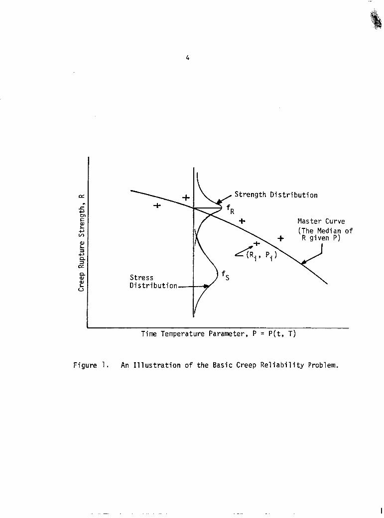
stress S, i.e., .(R<S). The latter definition is adopted here. Figure 1

illustrates the baslc problem. Both creep strength and applied stress are

considered to be random variables. The risk or probability of failure is

defined as

pf = Pr (R < S> (3)

To evaluate p it is necessary to establish the statistical distribution of

R and S. The process of development of the functional relationship between

strength and the TTP also addresses the problem of translating the creep-

rupture data into a statistical distribution of R. The basic relationship

proposed here for creep strength is called the "exponential model,"

f'

loglOR = A + BPm ( 4 )

A , B, and IUI are parameters to be determined from the data.

Note: In the case of the LM parameter the value of the parameter P used

in the exponential model is in thousands, while for the MH parameter the

absolute value of P is used. In the range of interest, P is a negative

valued function which can not be raised to a rational power.

The median curve of R given P can be established by a least squares

analysis. The model parameters A , B and m are calculated by an iterative

procedure. Note that if m is considered a constant, best linear unbiased

estimates of the parameters A and B can be calculated by applying a least

4

Stress Distribution-

Strength Distribution

+ Master Curve (The Median o f + R given P)

Time Temperature Parameter, P = P(t, T)

Figure 1. An Illustration o f the Basic Creep Reliability Problem.

. I

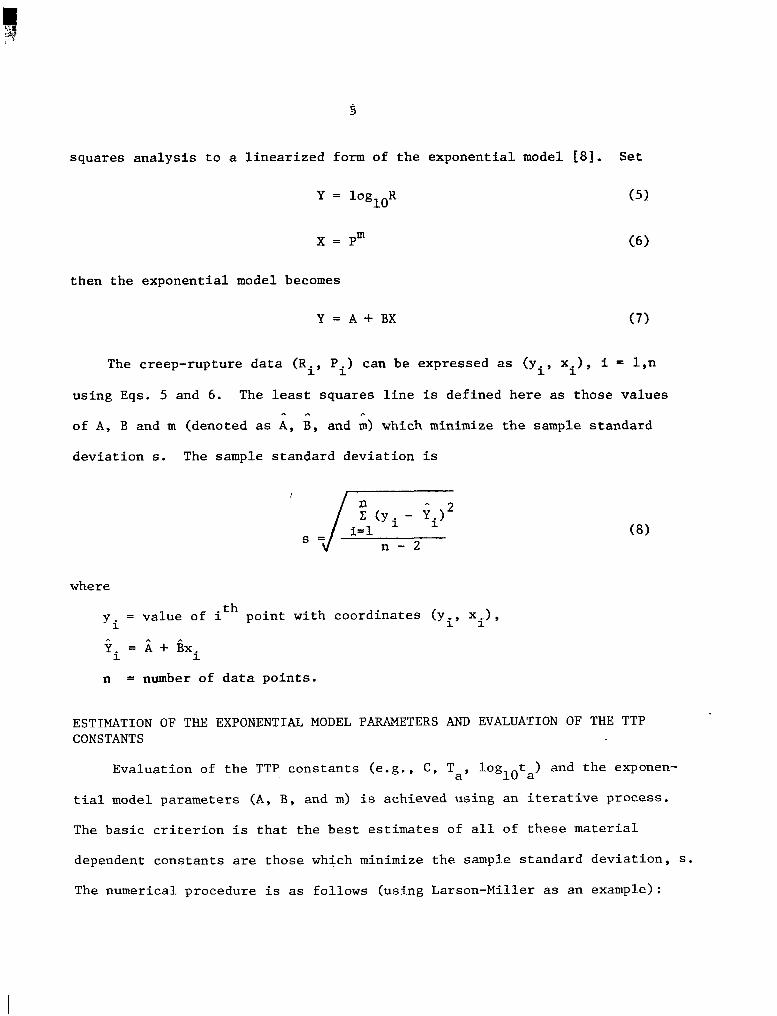
squares analysis to a linearized form of the exponential model 181. Set

Y = log loK ( 5 )

x = Prn

then the exponential model becomes

Y = A + BX (7)

The creep-rupture data (Ri, Pi) can be expressed as (yi, xi>, i = 1,n

using Eqs. 5 and 6 . The least squares line is defined here as those values

of A, B and m (denoted as A, B, and m) which minimize the sample standard

deviation s. The sample standard deviation is

A , . ,-.

, . 2 J * n - 2

c (Yi - Yi) i- 1

s =

where

'i = value of ith point with coordinates (yi, xi),

n = number of data points.

ESTIMATION OF THE EXPONENTIAL MODEL PARAMETERS AND EVALUATION OF THE TTP CONSTANTS

The basic criterion is that the best estimates of all of these material

dependent constants are those which minimize the sample standard deviation, S.

The numerical procedure is as follows (using Larson-Miller as an example):

6

1.

2.

3.

4 .

5.

6 .

7.

Choose an initial value of C.

Choose an initial value of m.

Use the simple least squares analysis to compute A and B.

Compute s (Eq. 8 ) .

Repeat steps 2 through 4 until an m is found (corresponding to your

initial choice of C) which minimizes s .

Going back to step 1, repeat the process using another value of C.

Finally, this procedure produces a minimum s as a function of C.

The "best" estimate of C is defined as that value which corresponds

to the minimum value of s . The corresponding values A, fi, and

are estimates of m, A, and B respectively.

4 A

This procedure is easily extended to the case of two (or more) constants.

For the MH parameter, steps 1, 6 , and 7 are extended to accomodate two

constants.

Finally, the "optimum" master curve is

A

l0g1()fi = ii + ipm

Examples of this analysis applied to a sample of n = 95 Incoloy 625 data

are provided in Figs. 2 (for LM) and 3 (for MH) . The coherence of the data to the master curve is measured by CR, the coefficient of variation of R

(praportional to S: as given by Eq. 11 below) which defines the vertical

scatter. The fact that the MH analysis produces a slightly lower CR suggests

a slightly better fit, . . . not surprising in view of the additional con- stant in the MH parameter.

Table 1 is a summary of the results obtained from an exponential model

analysis for five materials. The significance of these results lies in

Fig. 2. Example o f Proposed Analysis Procedure Applied to Incoloy 625 Creep-Rupture Data Using

Larson-IYI 11 e r Parameter.

INCOLOY 625 n 0

I

Sample Size, n = 95 Sample Std. Dev. s = 4.62E-2 Coeff. of Variation, CR = 10.68 C = 25.05

3

-

3

0 0 d l I I I I I 1

25.0 30.0 35.0 40.0 45.0 50.0 55.0 60.0

pl .7!

0 0 d

I I

25.0 36.0 3;. 0 40.0 45. 0 50. 0 55.0 ,o L-M PARAMETER (KS)

Fig. 3. Example o f Proposed Analysis Procedure Applied to Incoloy 625 Creep-Rupture Data Using the Manson-Haferd Parameter.

INCOLOY 625

Sample S i z e , n = 95 Sample S t d . Dev., s = 4 . 1 E-2 Coeff. o f Variation o f R , CR = 9.46%

T = 594OF loglOta = 15 .8

a

M-H PRRRMETER

- 5.7683-03 P 1 .307

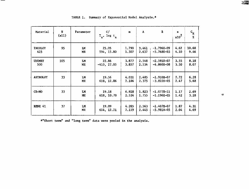
TABLE 1. Summary of Exponential Model Analysis.*

INCOLOY ~ 95 625

UDIMET 105 500

ASTROLOY 33

CR-MO 33

RENE 41 37

*"Short term" anc

Parameter LT ~~

LM 594, 15.80 MH 25.05

-410, 27.05 MH 22.86 LM

LM 618, 12.86 MH 19.56

LM 19.18 MH 618, 10.70

LM 614, 12.21 MH 19.09

"long term" data were pooled j

1.790 1.307

10.68 4.62 -1.7963-09 3.461 9.46 4.10 -5.7683-03 2.637

3.877 3.857

8.18 3.55 -2.591E-07 2.548 8.07 3.50 -4.8603-08 2.534

I I I I

4.031 2.485 -1.910E-07 6.28 2.186 I 2.375 I -3.8223-05 I x::: I 5.68

6.928 1.823 -1.0773-11 1.17 2.69 2.534 I 1.755 I -1.1963-05 I 1.42 I 3.28

I I I I

I 4.205 2.563 -1.4073-07 4.31 2.119 1 2.445 1 -5.9813-05 I i::: 1 4.69

I I I I

tn the analysis.

W

10

the demonstration that typical values of CR are less than 10%. This value

includes both scatter in material behavior and modelling error associated

with the use of a TTP. Note that in comparison, scatter in room temperature

static properties for most metallic materials is characterized by coefficients

of variation of 5 to 10%. Finally, note that the R-P data for all the

materials of Table 1, when plotted, would exhibit the same coherence to

the master curve as those of Figs. 2 and 3.

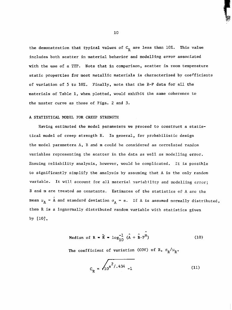
A STATISTICAL MODEL FOR CREEP STRENGTH

Having estimated the model parameters we proceed to construct a statis-

tical model of creep strength R. In general, for probabilistic design

the model parametera A , B and. m could be considered as correlated random

variables representing the scatter in the data as well as modelling error.

Ensuing reliability analysis, however, would be complicated. It is possible

to significantly simplify the analysis by assuming that A is the only random

variable. It will account for al.1 material variability and modelling error;

B and m are treated as constants. Estimates of the statistics of A are the

mean u = A and standard deviation uA = s. If A is assumed normally distributed,

then R is a lognormally distributed random variable with statistics given

h

A

by [IO],

A

Median of R = R = log (A + B*Pm) % -1 A A

10

The coefficient of variation (COV) of R,

11

Note that the master curve of Fig. 2 is in fact R. Also note, as stated

above, that cR = 12.3%, given on the figure, is a measure Of the vertical

scatter.

'L

This form of computing CR ignores the statistical scatter of the esti-

mates. However, it has been found that in the elementary least equares

case, the distribution of the estimators does not play a significant role

for sample sizes of roughly n > 30 [lo]. For the many available creep-

rupture data sets of this size or larger, the statistical distribution

of the estimates is not expected to be significant.

BIAS AND UNCERTAINTY IN PREDICTING LONG TERM BEHAVIOR FROM SHORT TERM DATA

The ability of a TTP to predict long time behavior (e.g., 20 to 40

Years) from short time data (e.g., less than 1 year) is of special interest

to designers. A parameter which provides accurate predictions of long

time properties would improve current design practices by reducing the

risk and/or avoiding overdesign. The ability of a TTP to predict long

time behavior can be measured by (a) constructing a model using short

term data only, and (b) comparing long term data with the model predictions.

Define A as the ratio of observed to predlcted behavior; A f.s an index

which defines the quality of a model. Following is a mathematical predic-

tion of A in a form which is suitable for probabilistic design purposes.

Define ,

ROBS (i)

%RE (i)

= Observed strength (long term data) of ith specimen

= Predicted strength of ith specimen (model based on short term data only)

n = number of long term data points

12

Define A associated with the ith specimen as,

But A i , in general, will be different for each test specimen. Therefore,

A will be a random variable. Compute the sample mean and sample standard

deviation as,

i=l

It is assumed that A will have a lognormal distribution. In fact, statis-

tical tests (not reported here) show that A seems to follow an approximate

lognormal distribution for many data sets. The median and COV of a lognormal

A will be respectively [lo],

C ,, = sA /A -

Note that Chmeasures both scatter in material behavior and strength

modelling error. The closern is to unity and the smaller is sA , the better

the predictions. If A < 1, then the model has a tendency to overestimate -

long time strength. For 1\ > 1 the strength is underestimated.

13

Tables 2 and 3 summarize an exercise to study the behavior of A from

typical creep-rupture data. Models based on the short term data are sum-

marized in Table 2 for various data sets. The bulk of the short term

data is less than 1000 hours, with only a few points between 1000 and

3500 hours. Then the mean and COV of the bias in predicting long term

behavior for each data set is summarized in Table 3. Lives of most of

the long term data were from 12 to 18 months. The short term and long

term data used here was provided by Goldhoff (7). Note that the MH param-

eter seems to perform much better than the LM parameter as evidenced by

the fact that 7 is consistantly closer to one.

RELIABILITY ANALYSIS

In general reliability analysis,one should consider all sources of

uncertainty including data scatter as well as the bias and distribution of

modelling error. Material data scatter is described by the random variable

A in the creep rupture analysis. But the bias A contains both scatter

in material behavior and modelling error. In addition, temperature T

and stress S can be treated as random variables reflecting uncertainties

in the environment as well as the analysis. The goal of reliability

analysis is to synthesize statistical information to compute risk.

For a practical reliability analysis we need an estimate of the

I 1 in service" strength which accounts for data scatter as well as predictive

capabilities of the model. Define the actual strength of the material

Ra 9

R = Y R a

TABLE 2. Summary of the Analysis of Short Term Data.

I

Material A m C Parameter N (short

1% t, time) Ta (OF) 9

I#%oloy 2.377 1.221 815, 13.40 MH

3.698 1.616 32.11 LM . 78 625

UDIMET 2.534 3.954 24.11 L? 93 500 MH 2.540 4.108 -545, 29.24

LM 500

26.27 L4:: 2.462 -554, 30.50 2.470

I

ASTROLOY 2.324 5.084 24.60 LM 21 MH 2.236 2.853 600, 14.71

RENE 41 2.505 4.582 20.34 LM 26 MII 2.395 2.360 609, 12.08

CR-MO 1.852 6.484 20.57 LM 23 MH 1.756 2.592 618, 10.17

HASTELLOY 4.683 0.940 18.59 LM 29 X MH 2.905 0.834 614, 11.08

r 316-SS 2.337 2.746 17.93 LM 28

MH 2.106 1.414 618, 10.06

L-605 2.167 3.210 18.79 LM 76 MH 2.050 1.761 583, 17.27

A1-1100 2,274 1.056 18.04 LM 53 MH 2.355 1.056 -499, 22.92

B

-2.7373-03 -7.5263-03

-1.549E-07 -1.749E-08

-1.6433-08 -2.5173-09

-9.5703-10 -2.2403-06

-2.4763-08 -1.8083-05

-3.701E-11 -7.8783-06

-1.0823-01 -3.7773-02

-5.7143-05 -1.4443-03

-5.4763-06 -2.1133-04

-8.968E-02 -3.5693-02

Time less

I I 1 I t

4.19 9.68 145 1 3.84 I 8.86 I

1.88

1.69 1.83

0.867 0.843

3.54 3.54

1.26 1.35

1.92 2.50

I 1.34 1.42

8.30 139 8.34

3.72 23 4.43

3.89 32 4.22

2.00 90 1.94

8.16 37 8.18

2.89 38 3.12

4.42 40 5.75

3.08 17 3.28

15

TABLE 3 . Statistics of A Exhibited by the TTP's.

MATERIAL Number of Data Points LM I MH

INCOLOY 625

UDIMET 500

UDIMET 500

ASTROLOY

RENE 41

CR-MO

HASTELLOY-X

316-SS

L-605

A1-1100

x 0.477

0.928

0.904

0.884

0.971

0.967

0.920

1.037

0.668

1.036

~ ""

. .

~~ ~ ~

~~~ -

C % n ji C % A Short Time

15.6

21 8.65 0.928 9.52

66 6.93 0.939 7.69

93 3.95 0.972 5.27

78 12.00 0.941

15.6 0.993 19.0

6.07 1.055 . .

Long Time

17

12

37

12

11

10

18

10

28

11

16

where Y is a random variable which accounts for bias and uncertainty of

modelling error associated with using a TTP to extrapolate. R is the predicted

strength of the material as calculated from the exponential model, Eq. 4, as

R = loglo (A + BPm) -1 (18)

where P = P(t ,TI. R is a random variable because A and T are random vari-

ables. Note that if T is assumed to be constant and A is normally dis-

tributed, then R would have an exact lognormal.

The statistics of '4 are established as follows. First it is assumed

that T = constant in the data used to compute A and q. Then assume that 'L

Y is lognormal. R will have exact lognormal with statistics a

'L ' L ' L Median, Ra = Y R

cov, c = /(1 + CG) (1 + Ci) - 1 (20) Ra

Nowh contains both data scatter and modelling error so that CR = CA.

Also note that a

Comparing Eqs . 19 and 2 1 and solving for CA in Eq. 20, the statistics

for A are ' L ' L

Y = A

c 1 + CA

"1 + CR

What we have done is to extract uncertainty due to modelling error from

A . Thus, C describes modelling error in the use of the TTP. Y

17

Consider a simple example which illustrates how to separate material

variability from modelling error associated with using a TTP to extrapolate

to long t2mes. Use of the LM parameter on Incoloy 625 is demonstrated.

CR is established from short term data as 0.0968 (See Table 2). From long

term data (Table 3 ) , = 0.477 and CA = 0.156. The median of A is computed

from Eq. 15 as A = 0.471. Thus, Y = 0.471. From Eq. 22, Cy = 0.121.

Thus, statistics on modelling error and material behavior are separated.

% %

It should be noted that C >, C with equality when there is no modelling A R

error due to extrapolation. The fact that CR exceeds C in some of the

data sets of Table 2 and 3 , suggests that sample sizes were inadequate. A

Furthermore, note that CR contains some modelling error. The use of a

TTP to describe a complex material phenomena suggests only an approxima-

tion to physical reality. However, because the values of C (less than 10%)

do not significantly differ from those of other static properties, it is R

likely that this component of modelling error is small.

If both the distributions of stress, S and R are lognormal, a closed a

form expression for probability of failure is available [lo]. The proba-

bility of failure is

Pf = @ (-5)

where 0 is the standard normal cdf,and f3 is the safety index, as given by

%

S and Cs are the median and COV of S respectively.

18

In the more general case where T is also considered to be a random vari-

able, reliability analysis becomes much more difficult. Techniques such as

Monte Carlo or Rackwitz-Fiessler method [ lo , 121 must be employed to relate risk to the design parameters.

It is important to note that computed values of p should be considered f

as "notional" values of the probability of failure. Because of the many

uncertainties and assumptions and because risk levels are so low, it may be

imprudent to argue that pf defines risk levels in an actuarial sense.

DEMONSTRATION OF RELIABILITY ANALYSIS

Example 1. It is required to design a tension element to the following

specifications (a) the temperature is llOO'F (593'C), (b) the life of the

component is 40 years (350,000 hrs), (c) the applied load is lognormally

distributed with statistics P = 10 kips (44 .48 KN) and Cp = 25%. The materi- QJ

al considered is Hastelloy X. The problem is to find the component's minimum

cross-sectional area A if the maximum allowable risk is p = 10 . From normal 4 f

tables the target safety index is B = -0-l(pf) = 3.72 . In this problem

both the LY and MH parameters will be used. The relationship of load to

stress is S = P I A , hence C s = Cp = 25%.

a) Larson-Miller Analysis

The optimized form of the LM parameter for Hastelloy X is given

by (See Table 2)

P = (1100 + 46O)(loglO 350,000 + 18.59) = 37.65 thousands

19

Using the da ta f rom Table 2 i n Eq. 4 , p red ic t ed s t r eng th is

loglo% = 4.683 - 0.1082 (37.65) 0.940

3 = 25.48 ks i (175.7 MPa)

The median and COV o f t h e a c t u a l s t r e n g t h Ra is o b t a i n e d u s i n g t h e d a t a

of Table 3. Note tha t (a) both model l ing e r ror and material behavior

are included and (b) the median of A is obta ined us ing Eq. 15.

CRa = CA = 15.6%

,-b Ra=AR =0.909 25.48 ksi = 23.16 k s i (159.67 MPa)

Rearranging Eq. 24, is given by %

Ra

exp {BIkn(l + CRa) (1 + C , ) l 1 51= 2 2 %

Then,

?J= 23.16 2 2 % = 7.82 k s i (53.91 MPa)

exp {3..72[kn(l + .156 ) (1 + .25 ) ] 1

For a s a f e d e s i g n t h e minimum requ i r ed area is

lo = 1.28in (8.25 cm ) 2 2 A ' s = 7 x 2

b) The Manson-Haferd Analys is

f o r H a s t e l l o y X is given by (see Table 2) The MH parameter

P =

Using data from Table 2 i n Eq. 4 , p red ic t ed s t r eng th is

10% ,8 = 2.905 - 3.7773-02 (87.8) 0.834

% R = 21.25 k s i (146.51 "a)

20

The median and COV of the actual strength is obtained from Table 3.

A is computed using Eq. 15. %

CRa = c, = 19.0%

%a = A R = 0.979 21.25 ksi = 20.8 ksi (143.40 MPa) % %

Then, as above, the maximum allowable stress is

n.8 20.8 s = = 6.55 ksi (45.18 ma) exp I3.72 [h(l + .1g2)(1 + .2l2)I4}

For a safe design, the requirement on the area is

2 2 A 1 PIS = 1016.55 = 1.53 in (9.85 em

We are incapable of providing a commentary at this point regarding

the poor agreement between the design as established by each parameter.

From intuition, however, it seems reasonable to place more confidence in

MH simply becuase it contains two (rather than one) empirical constants.

Example 2. As an extension to Example 1, assume now that uncertainties

in the temperature analysis are to be considered. It is estimated that

the median (best estimate) of T is llOO'F and COV of T is 5%. The member

chosen has a cross sectional area of 1.60 in2 (10.3 cm ) , larger than the

1.53 in2 (9.85 cm ) required in the constant T case. Does the design

2

2

satisfy the basic requirement that the target safety index, 8 > 3.72?

A closed form solution is not available. To solve this problem, a

numerical method, the Rackwitz-Fiessler (R-F) method will be employed

[lo, 121. The computer program requires the limit state as input.

(S = YR) = (S = Y log;; {A + B [ (T + 460) (loglot 18.59)]m}

21

S, A and T are random variables. It is clear that the computation

of the probability of failure event would be most difficult by classical

methods.

The computations are summarized in Table 4 . The computed safety

index, B = 3 . 3 3 , is less than the target safety index f 3 = 3 . 7 2 , so the

design is considered to be unsafe. It is interesting to note that if

we let C + 0 (T = ?, a constant), then the safety index is f3 = 4 . 5 0 .

Clearly reliability is sensitive to uncertainties in T.

0

T

We can also compute the notional probability of failure as

For 6 = 3 . 3 3 , pf = 4 . 3 6 E - 4 , and for f 3 = 4 . 5 0 , pf = 3.44E-6 .

CONCLUSIONS

A general method for reliability analysis of creep rupture data is

presented. The method employs the time-temperature parameter (TTP) concept.

An exponential mode1,log R = A + B P ,relating strength R, to P, the TTP, was shown to provide a good fit to creep-rupture data. Evidence of

the quality of the exponential model is provided by the low values of the

coefficient of variation of R in Table 2 (typically less than 10%). Further-

more, the exponential model fits well into a probabilistic design format.

m 10

In general, the assumption that all of the statistical scatter of

the data can be lumped into A is valid only when the data is homoscedastic

(constant scatter band). This data is not always homoscedastic when the

Universal constants associated with each TTP are used.

22

(a) TABLE 4. Summary of the Input and Output of the UA Reliability Program to Calculate B.

0 Data ~~

Variable 0 COV% Median Mean Distribution

S 25 .O 6.25 Lognormal - A 6)

~~~ .

Normal 0.382 8.2 4.683 ~~ ~

T 5.0 1100 Lognormal

Y 13. 3(d) 0.909(c) Lognormal

0 Safety Index, B = 3.327

Notional Probability or Failure, Pf = 4.40E-4

0 Design Point (approximately most probable value on the limit state function; close to the peak of the joint probability density function of the design factors) * s = 7.57

A* = 4.674

T = 1329

Y = 0.857

* *

Notes

(a) This program has the option of using the Hasofer-Lind, Rackwitz-Fiessler or Chen-Lind method for computing the generalized safety index.

(b) Hastelloy X; See Table 2.

(c) Y = A ; and A obtained using Eq. 15 and data of Table 2. % % %

(d) Computed using data of Tables 2 and 3 and Eq. 22.

23

The assumption that A is normally distributed is a matter of con-

venience for the reliability analysis. While no formal goodness of fit

test was used, the normal assumption for A seems to be very reasonable

on the basis of visual inspection of R-P plots.

Investigation of the bias in predicting long term behavior from

short term data of both the LM and MH parameters suggest that both do a

fair job. But no general trend was observed. Probability plots of A ,

and hence Y , suggest that A (and Y ) follows a distribution close to a log-

normal.

Finally, failure is not always defined as rupture. It can be defined

as excessive deformation. When this is the case, a similar approach to

the one presented above is possible. Time to failure would indicate time

to achieve a predetermined deformation, say 1, 2, or 5% creep, Creep

strength would now be defined as stress, e.g., for 1, 2, or 5% creep

strain. Fig. 4 illustrates the master curves for creep rupture and 1% strain.

I

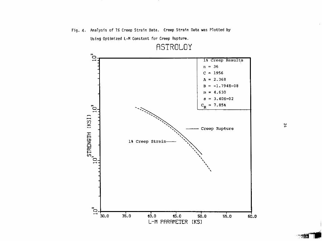
Fig. 4 . Analysis of 1% Creep Strain Data. Creep Strain Data was Plotted by

Using Optimized L-M Constant for Creep Rupture.

ASTROLOY 1% Creep Results n = 36 C = 1956 A = 2.368 B = -1.7943-08 m = 4.630 s = 3.403-02

CR = 7.85%

\ '. ' \ \ \

n I - 0 1 4' 1 I I 1 I

30.0 35.0 40.0 45.0 so. 0 55.0 L-M PARAMETER (KSI

I. 0

25

REFERENCES

1.

2.

3.

4.

5.

6.

7.

8.

9.

10.

11.

12.

13.

Larson, F. R. and Miller, J., "A Time-Temperature Relationship for Rupture and Creep Stress," Transactions ASME, Vol. 74, 1952, p. 765.

Manson, S. S. and Haferd, A. M., "A Linear Time-Temperature Relation for Extrapolation of Creep and Stress Rupture Data," NACA TN 2890. 1953.

Orr, R. L., Sherby, 0. D. and Dorn, J. E., "Correlation of Rupture Data for Metals at Elevated Temperatures," Transactions ASME, Vol. 46, 1954, p. 113.

Manson, S. S., "Time Temperature Parameters - A Re-evaluation and Some New Approaches," ASM Publication No. D8-100, 1968.

Conway, J. B., Stress-Rupture Parameters: Origin Calculation and - Use, Gordon and Breach, Science Publishers, Ltd., London, 1969.

Grounes. M., "A Reaction Treatment of the Extrapolative Methods in Creep Testing," Transactions ASME, Journal of BHsic Engineering, March 1969, p. 59.

Goldhoff, R. M., "Towards the Standardization of Time-Temperature Parameter Usage in Elevated Temperature Data Analysis,'' Journal of Testing and Evaluation, JTEVA, Vol. 2, No. 5, Sept. 197, pp. 387-424.

Hines, W. W. and Montgomery, D. C., Probability and Statistics in Engineering and Management Sciences, John Wiley & Sons, New York, 1980.

Manson, S. S. and Ensign, C. R., "A Quarter Century of Progress in the Development and Extrapolation Methods for Creep Rupture Data." Journal of- Engineering Maierials and Technology, Vol. iOl, Oct . 1979, p. 317.

Wirsching, P. H., "Application of Probabilistic Design Theory to High Temperature Low Cycle Fatigue," NASA CR-165488, NASA Lewis Research Center, Cleveland, OH., Nov. 1981.

Hahn, G. J., "Statistical Methods for Creep, Fatigue and Fracture Data Analysis," Transactions ASME, Journal of Engineering Materials and Technolopy, Vol. 101, Oct. 1979, pp. 344-348.

Thoft-Christensen, P., Baker, M. J., Structural Reliability Theory and Its Applications, Springer-Verlag, N. Y., 1982.

Wu, Y. T., McLain, S. D., Kelly, C. F., and Wirsching, P. H., "On the Performance of the Rackwitz-Fiessler and Chen-Lind Algorithms for Computing Structural Reliability," The University of Arizona, Sero. and Mech. Engr. (manuscript in preparation), 1983.

26

14. Clough, W. R. and Kaut, P. K., "Computerized Evaluation of the Rela- tive Properties of Seven Time Temperature Parameters to Correlate and Extrapolate Nickel Alloy Stress-Rupture Data," Transactions ASME, Journal of Basic Ennineerinpl, March 1972, p. 7.

15. Goldhoff, R. M., "Comparison of Parameter Methods of Extrapolating High Temperature Data," Transactions ASME, Journal of Basic Engineering, Dec., 1959, p. 629.

16. Manson, S. S. and Ensign, C. R., "Interpolation and Extrapolation of Creep Rupture Data by the Minimum Commitment Method - Part I - Focal- Point Convergence," NASA TM-78881, 1978.

17. Manson, S. S. and Ensign, C. R., "Interpolation and Extrapolation of Creep Rupture Data by the Minimum Commitment Method - Part I1 - Oblique Translation," NASA TM-78882, 1978.

18. Manson, S. S. and Ensign, C. R., "Interpolation and Extrapolation of Creep Rupture Data by the Minimum Commitment Method - Part I11 - Analysis of Multiheats," NASA 'I'M-78883, 1978.

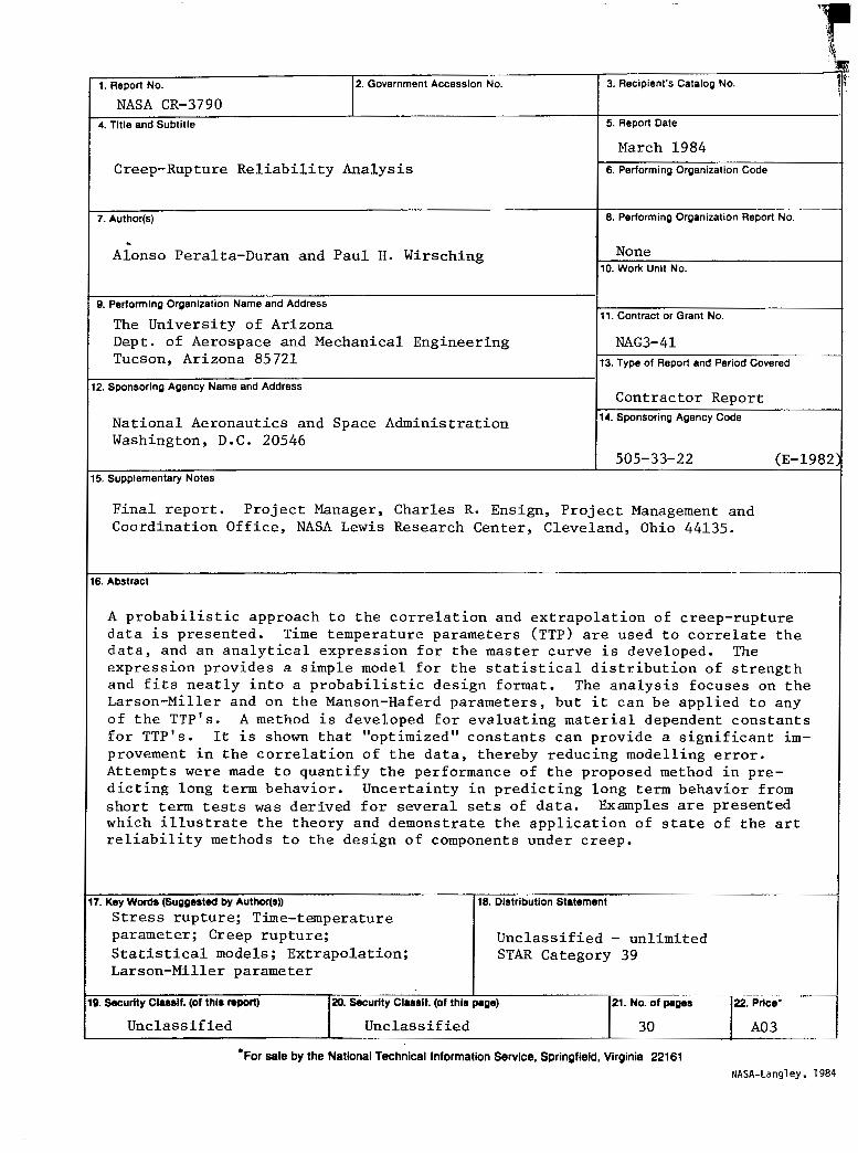
1. Report No. 2. Government Accession No. 3. Recipient's Catalog No.

NASA CR-3790 4. Title and Subtitle 5. Report Date

Creep-Rupture Reliability Analysis 6. Performing Organization Code

7. Author(s) 8. Performing Organization Report No. "_

.. Alonso Peralta-Duran and Paul H. Wirsching 1 10. Work Unit No.

9. Performing Organization Name and Address

The University of Arizona Dept. of Aerospace and Mechanical Engineering Tucson, Arizona 85 721

NAG3- 41

11. Contract or Grant No.

- 13. Type of Report and Period Covered

2. Sponsoring Agency Name and Address Contractor Report

National Aeronautics and Space Administration 14. Sponsoring Agency Code

Washington, D.C. 20546 505-33-22 (E-1982

5. Supplementary Notes

Final report. Project Manager, Charles R. Ensign, Project Management and Coordination Office, NASA Lewis Research Center, Cleveland, Ohio 44135.

6. Abstract

A probabilistic approach to the correlation and extrapolation of creep-rupture data is presented. Time temperature parameters (TTP) are used to correlate the data, and an analytical expression for the master curve is developed. The expression provides a simple model for the statistical distribution of strength and fits neatly into a probabilistic design format. The analysis focuses on the Larson-Miller and on the Manson-Haferd parameters, but it can be applied to any of the TTP's. A method is developed for evaluating material dependent constants for TTP's. It is shown that "optimized" constants can provide a significant im- provement in the correlation of the data, thereby reducing modelling error. Attempts were made to quantify the performance of the proposed method in pre- dicting long term behavior. Uncertainty in predicting long term behavior from short term tests was derived for several sets of data. Examples are presented which illustrate the theory and demonstrate the application of state of the art reliability methods to the design of components under creep.

7. Key Word8 (Suggested by Author(8)) 18. Dlstibutlon Statement ~~

Stress rupture; Time-temperature parameter; Creep rupture;

Larson-Miller parameter STAR Category 39 Statistical models; Extrapolation; Unclassified - unlimited

D. Security ClMSlf. (Of thl8 rOpofi) 20. Security ClM8lf. (Of thi8 page) " "-

21. No. of paws 22. Price' __ . ;; ~-

Unclassified 30 I A03 Unclassified

*For sale by the National Technical Information Service, Springfield, Virginia 22161 NASA-Langley. 1984