CreditRisk+ by Fast Fourier Transform Mario R. Melchiori

CreditRisk+ by Fast Fourier Transform

Mario R. Melchiori, CPA (*) 1

Universidad Nacional del LitoralSanta Fe - Argentina

First Version September 2002

This version July 2004

ABSTRACT

This paper focuses on the methodology described in CreditRisk+ Technical Document. Appendix A provides analytical explanations of the techniques used to generate the loss distribution arising from a credit portfolio. It is worth mentioning that although the underlying concepts are easy to grasp for those with an intermediate mathematical background, the notation used in this paper may bother those who are not fully familiar with it. First, we concentrate on the concepts surrounding Probability Generating Functions and Convolution, and their application within CreditRisk+. Then, we explain, in practical terms, the use of the recurrence relation as used in CreditRisk+. Lastly, we develop an alternative way for calculating credit losses with CreditRisk+ via the Fast Fourier Transform (FFT). In order to close the gap between theory and practical implementation we provide VBA, MatLab and R codes that present step-by-step examples of practical applications.

(*) BICA Coop. E.M.Ltda. 25 de Mayo 1774 – Santo tomé –SANTA FE- Argentina - E-mail: mrmelchi@grupobica.com.ar The opinions expressed in this paper are those of the author and do not necessarily reflect views shared by BICA Coop. E.M.Ltda. or its staff.

1 I am grateful to Anabella Boselli, Carina Strada and Luciano Alloatti for their generous contribution. I want to thank to Craig Nelson for helping me to translate this

paper and the files from Spanish to English. All remaining errors are, of course, my own.

(c)YieldCurve.com 2004

CONTENTS

1. INTRODUCTION......................................................................................................................................................................3 2. PROBABILITY GENERATING FUNCTION........................................................................................................................3

2.1 DISCRETE PROBABILITY DISTRIBUTION ...........................................................................................................................3 EXAMPLE 2.1: ................................................................................................................................................................................... 3 EXAMPLE 2.2: ................................................................................................................................................................................... 3 EXAMPLE 2.3: ................................................................................................................................................................................... 3 EXAMPLE 2.4: ................................................................................................................................................................................... 4

2.2. CONVOLUTION ......................................................................................................................................................................4 EXAMPLE 2.5: ................................................................................................................................................................................... 4

2.2.1. Convolution by Probability Generating Function: .......................................................................................................4 EXAMPLE 2.6: ................................................................................................................................................................................... 4 EXAMPLE 2.7: ................................................................................................................................................................................... 4 EXAMPLE 2.8: ................................................................................................................................................................................... 4

2.2.2. Convolution by FFT......................................................................................................................................................5 2.2.2.1 Auxiliary Functions.....................................................................................................................................................5 2.2.3 FFT Algorithm of convolution .......................................................................................................................................6 2.2.4 Frequency and Severity of Cumulative Losses...............................................................................................................6 2.2.5 Algorithm for computing the aggregate loss distribution by FFT .................................................................................6

3. CREDITRISK+: BASIC MODEL............................................................................................................................................7 3.1 PROBABILITY GENERATING FUNCTION ..................................................................................................................................7 OF A POISSON DISTRIBUTION. .......................................................................................................................................................7

EXAMPLE 3.1: ................................................................................................................................................................................... 7 EXAMPLE 3.2: ................................................................................................................................................................................... 8 Using the probability generating function concept, (2.28) and(3.8):............................................................................... 8 Using the recurrence relations of CreditRisk+, namely (3.9) and (3.10), we obtain: ............................................... 8 Using algorithm 2.2.3: .......................................................................................................................................................................... 9 EXAMPLE 3.3: ................................................................................................................................................................................... 9 Using algorithm 2.2.3: .......................................................................................................................................................................... 9 Using algorithm 2.2.5: .......................................................................................................................................................................... 9 Using the recurrence relation of CreditRisk+ (3.9) and (3.10):.............................................................................................................. 9

4. CREDITRISK+: EXTENSIONS OF THE BASIC MODEL ...............................................................................................10

4.1 RANDOMNESS OF THE RATE OF DEFAULT: ONE SECTOR.......................................................................................................10 4.1.1 Distribution of default events.......................................................................................................................................10

EXAMPLE 4.1: ................................................................................................................................................................................. 10 Using algorithm 2.2.5: ........................................................................................................................................................................ 11

4.1.2 Distribution of default losses for a portfolio................................................................................................................12 EXAMPLE 4.2: ................................................................................................................................................................................. 12 Using algorithm 2.2.5: ......................................................................................................................................................................... 12

4.2 SEVERAL SECTORS ...............................................................................................................................................................14 4.1.2 Loss Distribution using FFT........................................................................................................................................14

EXAMPLE 4.3 .................................................................................................................................................................................. 15 Using algorithm 2.2.3: ........................................................................................................................................................................ 15

5. CREDITRISK+ BY FFT .........................................................................................................................................................16

EXAMPLE 5.1 .................................................................................................................................................................................. 16 5.1 BASIC MODEL OF CREDITRISK+: ..........................................................................................................................................17 5.1.1 BASIC MODEL ALGORITHM BY FFT ................................................................................................................................17 5.2 EXTENDED MODEL OF CREDITRISK+: ..................................................................................................................................17

5.2.1 One Sector ...................................................................................................................................................................17 5.2.2 Several Sectors.............................................................................................................................................................17

6. CONCLUSIONS.......................................................................................................................................................................18 7. REFERENCES.........................................................................................................................................................................18

(c)YieldCurve.com 2004 2

CreditRisk+ by Fast Fourier Transform Mario R. Melchiori

1. Introduction

Many publications related to the credit risk field have come out during the last ten years or so. Unsurprisingly, the different methodologies used today to measure Value at Risk – VaR - of a credit portfolio, such as CreditMetrics (JP Morgan, 1997), CreditRisk+ (Credit Suisse Financial Products, 1997), PortfolioManager (KMV, 1997) and McKinsey´s CreditPortfolioView (Wilson, 1997) were born in that period. Subsequent to such publications, the goals of the more recent literature were to outline each work’s peculiarities2 and to analyze the differences and similarities3. Other literature espoused the expansion of their applications4. Based on credit risk management’s popularity, quite a few Internet portals exclusively focused on the subject, while many others researched it deeply5, though not in an exclusive fashion6. In this paper, we focus on the methodology followed in the CreditRisk+ Technical Document. Its appendix A gives analytical explanations of the techniques used to generate the loss distribution arising from a credit portfolio. It is worth mentioning that although the underlying concepts are easy to grasp for those with an intermediate mathematical knowledge, the notation used in this paper may annoy those who are not fully familiar with. First, we concentrate on the concepts of the probability generating function and convolution, and their application to CreditRisk+. We then explain in practical terms the use of the recurrence relation used by CreditRisk+. Lastly, we develop an alternative way to calculate CreditRisk+ through the Fast Fourier Transform (FFT). In order to cover the gap between theory and practical implementation we provide VBA, MatLab and R codes that present, step-by-step, all practical applications covered in this paper.

2. Probability Generating Function7

In this section, we introduce some basic concepts related to discrete probability distribution.

2.1 Discrete Probability Distribution

Let X be a discrete random variable defined on non-negative integers, 0,1,2. The random variable X can be fully described by a probability vector:

( ) ( ) ( ) ( )Xf 0 , 1 , 2 ,..., ,X X X Xf f f f R⎡ ⎤= ⎣ ⎦ (2.1)

or simply:

[ ]X 0 1 2f , , ,..., ,Rf f f f= (2.2)

with . In this representation, the

maximum possible value of X cannot exceed R. When R is finite, X has infinitely many vector representations of the form

( ) { }xf Prii f X i= = =

2 Crouhy, Galai & Mark (1998) 3 Koyluoglu & Hickman (1998), Christopher C. Finger (1998), Gordy (2000), 3 Bügisser, Kurth, Wagner & Wolf (1999) 5 For examples, see DefaultRisk.com 6 For examples, see e-Risk.com7 Here, we followed almost literally Aggregation of Correlated Portfolio, Models and Algorithms, Shaun S. Wang, section 2, page 851.

[ ]0 1 2, , ,..., ,0,0,0,...,0Rf f f f , (2.3)

Where a number of zeros are added to the right. For a discrete variable with a probability vector X

[ ]x 0 1 2f , , ,..., ,Rf f f f= the probability generating function is

defined by the symbolic series: ( ) 0 1 2 3

0 1 2 3 ... ,RX RP t f t f t f t f t f t= + + + + + (2.4)

which is also the expected value of Xt . The variable may represent: X The number of obligors and the probability that they

default or not default during a given period of time, or The exposure in the obligors and the probability that

they default or not default during a given period of time. EXAMPLE 2.1: If a discrete variable has the following probabilities: N { } { } { }Pr 0 0.50 Pr 2 0.40 Pr 5 0.10N N N= = = = = =

(2.5)

then it can be represented by a vector: [ ]0.50,0,0.40,0,0,0.10,0,...,0 ,Nf = (2.6)

and it has a probability generating function: ( ) 2 50.50 0.40 0.10NP t t t= + + (2.7)

EXAMPLE 2.2: If a discrete variable has the following probabilities: K

{ } { } { }Pr 1 0.40 Pr 2 0.30 Pr 3 0.30K K K= = = = = = (2.8)

then it can be represented by a vector: [ ]f 0,0.40,0.30,0.30,0,...,0 ,k = (2.9)

and it has the probability generating function: ( ) 2 30.40 0.30 0.30KP t t t t= + + (2.10)

EXAMPLE 2.3: Let’s consider a portfolio with only one obligor. Suppose this obligor has an annual 8% unconditional probability of default. An individual obligor may default or not default, thus, the number of defaults that may take place in the portfolio by the end of the year shall have the following probability distribution:

I

I

, { } { }Pr 0 0.92 Pr 1 0.08I I= = = = (2.11)

and it can be represented by the vector: [ ]If 0.92,0.08= , (2.12)

which has a probability generating function:

(c)YieldCurve.com 2004

. ( ) 0 1P t = 0.92t +0.08tI(2.13)

Formula (2.13) is equivalent to formula (3) of the CreditRisk+ Technical Document, although we introduce it as a function of t and not , as it appears in the document.

z

EXAMPLE 2.4: We can formulate the previous example in a different way. If we define the portfolio value as the event of interest, instead of the number of defaults, and considering the individual obligor with an exposure value of $10 and a recovery value of $0, we will find that at the end of the year the portfolio value shall have the following probability distribution:

P

, { }Pr 0 0.08P = = { }Pr 10 0.92P = = (2.14)

which can be represented by the vector: [ ]Pf 0.08,0,0,0,0,0,0,0,0,0,0.92= , (2.15)

which has the probability generating function: . ( ) 0 10.08 0.92PP t t t= + 0 (2.16)

2.2. Convolution Suppose and independent discrete random variables defined on non-negative integers. Let

N K

J N K= + represent the sum of N and . The probability distribution of

K

J represents the convolution of the probability distributions of and and is defined by: N K

{ } { } { }

0

Pr Pr Pr ,j

n

J j N n K j=

= = = = −∑ n

}

0,1,2,...,j n=

(2.17)

EXAMPLE 2.5:

For the random variable defined by equation (2.5) and (2.8) we have:

{ } { } { } {5

0

Pr 5 Pr 5 Pr Pr 5n

J N K N n K n=

= = + = = = = −∑ (2.18)

Since many of the terms are zero, we have: { } { } { }Pr 5 0 0 Pr 2 Pr 3 0 0 0 0.12.j N K= = + + = = + + + = (2.19)

22..22..11.. CCoonnvvoolluuttiioonn bbyy PPrroobbaabbiilliittyy GGeenneerraattiinngg FFuunnccttiioonn:: Note that: ( ) ( ) ( ). . .N K N K N K

N K N KP t t t t t t P t P t++ ⎡ ⎤ ⎡ ⎤ ⎡ ⎤ ⎡ ⎤= Ε = Ε = Ε Ε =⎣ ⎦ ⎣ ⎦ ⎣ ⎦ ⎣ ⎦

(2.20)

due to the independence of and K . In other words, the probability generating function of the sum N is the product of and .

NK+

( )NP t ( )KP t

EXAMPLE 2.6:

In terms of probability generating function for the random variable defined by equations (2.5) and (2.8), we have:

( ) ( ) ( ) ( ) ( )2 5 2. 0.5 0.4 0.1 0.4 .3 0.3J N KP t P t P t t t t t t= = + + + + 3 . (2.21)

After expansion we obtain:

( ) 2 3 4 5 6 70.20 0.15 0.31 0.12 0.12 0.04 0.03 0.03JP t t t t t t t t t= + + + + + + + 8

. (2.22)

The coefficient jt gives the probability that J = j. For example: . { }Pr 5 0.12J = =

EXAMPLE 2.7:

Let’s consider the portfolio with two obligors. We assume that one obligor has an annual unconditional probability of default of 8% and the other has an annual unconditional probability of default of 5%. Thus the number of defaults that may take place in the portfolio by the end of the year shall have the following probability distribution:

I

I

( ) ( ) ( )0 1 00.92 0.08 0.95 0.05IP t t t t t= + + 1 (2.23)

( ) ( )0 10.874 0.122 0.004IP t t t t= + + 2

P

. (2.24)

Equation (2.24) shall be interpreted as follows: There is a 0.4 % of probability that both obligors default, a 12.2 % of probability that only one obligor defaults, and an 87.4% of probability that neither obligors default, after one year. EXAMPLE 2.8:

The above example can be introduced using the portfolio value as the event of interest, instead of using the number of defaults; thus, if we assume that the exposure is $10 for the first obligor and $ 5 for the second, and further assuming a recovery value of $0 in both cases, the portfolio ´s value by the end of the year will have the following probability:

P

( ) ( ) ( )0 10 00.08 0.92 0.05 0.95PP t t t t t= + + 5 (2.25)

( ) ( )0 5 10 150.004 0.076 0.046 0.874PP t t t t t= + + + (2.26)

Once again, the above written a formula, which shall be interpreted in the following way. There is a 0.4% of probability that the portfolio ´s value is $0 (which means that both obligors have defaulted), a 7.6% of probability that portfolio ´s value is $5 (that is to say the obligor whose exposure was $5 did not default and the other obligor whose exposure was $10 did default), a 4.6% of probability that portfolio ´s value is $ 10 (which means that the obligor whose exposure was 10$ did not default and the one whose exposure was 5$ did default), and finally, an 87.4% of probability that portfolio ´s value is 15 $, (which is only possible if both obligors do not default by year end).

P

J

P

P

P

(c)YieldCurve.com 2004 4

As can be deduced, as long as the number of factors is reduced, we get the result of this formula quite easily. After multiplying the terms, we can expand the formula in t, and in doing so it is necessary to calculate the nth derivative of ,

evaluated at

( )P t

0t = . The result shall then be divided by the nth factorial. This process is equivalent to equation (20) of the CreditRisk+ technical document, except for the fact that we have assumed a binomial distribution for the event of default. Alternatively, CreditRisk+ assumes a Poisson distribution for

defaults, which allows one to find a simple recursive formula that, in turn, permits the calculation of the derivatives and factorials already mentioned. To introduce another example we now calculate the probability of loss suffered in the portfolio whose initial value at $10. We will assume a binomial distribution for the event of default. Thus, the probability generating function is: ( ) ( )0 10 00.92 0.08 0.95 0.05t t t+ + 5t . (2.27)

We now calculate the tenth derivative of (2.27) and divide it by ten factorial to obtain:

( ) ( )

100 10 00.92 0.08 0.95 0.05

10!

dt t t t

dt⎛ ⎞ + +⎜ ⎟⎝ ⎠

5

. (2.28)

The result of which is:

( )50.004 3003t +19 , (2.29)

and when evaluated at t = 0 yields: ( )50.004 3003.0 +19 = 0.076. (2.30)

This implies that the probability of suffering a portfolio loss of $10 during the year is 7.6%. If we take the case of formula (2.26)for t5 we will obtain the same result. This is due to the fact that in formula (2.26) the coefficient of t5 represents the probability that the portfolio is worth $5, whereas the result of formula (2.30) represents the probability that a portfolio loses $10. Formulas (2.26) and (2.30) are basically two different ways of representing the same event. Another way of arriving at this convolution is via the Fast Fourier Transform (FFT), which we will approach later in this paper, and which will help us to understand why CreditRisk+ uses the Poisson probability distribution instead of Binomial probability distribution. 22..22..22.. CCoonnvvoolluuttiioonn bbyy FFFFTT Before getting deeper into this subject, it is worth mentioning that there are several useful auxiliary functions associated with a distribution function of a

random variableY .

( )f x

1. Probability Generating Function 2. Moment Generating Function 3. Characteristic Function 4. Cumulam Generating Function

Given certain conditions, we can change from one auxiliary function to another. CreditRisk+ uses function 1, Finger8 uses the auxiliary function 2, Gordy9 uses function 4; and in this paper we use function 3.

22..22..22..11 AAuuxxiilliiaarryy FFuunnccttiioonnss The Univariate Case

8 CreditMetrics Monitor Abril 1999 ( Free registration required) 9 Saddlepoint Approximation of CreditRisk+ Published in Journal of Banking and Finance, 26(7), August 2002, pp. 1337-1355.

Let be a non-negative random variable of discrete, continuous, or mixed type. Let be the probability

(density) function of ,for example:

X

( )Xf x

X

( )( )

{ }Pr , if X is discrete

, if X is continuous{

X

X xX d

F xdx

f x == (2.31)

The Probability Generating Function of is defined by: X

( ) ( ) ( )( ) if X is discrete,

if X is continuous. { X

XX

X

f x tXX f x t dx

P t t ∑= Ε =∫

(2.32)

The Moment Generating Function of is defined by: X

( ) ( ) ( )tX t

X XM t e P e= Ε = (2.33)

The Characteristic Function, also called the Fourier

Transform of , is defined by: X ( ) ( ) ( )i i itX t

X Xt e P e Mφ ⎡ ⎤= Ε = =⎣ ⎦ X t , (2.34)

where i 1= − is the imaginary unit. The Cumulam Generating Function of is defined by: X

( ) ( )log X XK t M t= (2.35)

The Multivariate Case For a set of random variables ( ) , let be the

joint probability (density) function. For example:

1,..., kX X1,..., kX Xf

( ){ }

( )

1

1

1

,..., 1

1 1

,..., 1,...,

,...,

Pr ,..., , if the are discrete,

, if the are continuous....

k

k

k

X X k

k k j

k

x x k jx x

f x x

X x X x X

F x x X

=

= =

∂∂ ∂

For any subset of { }1, 2,..., kX X X their (joint) probability

distribution is called the marginal probability distribution of

1 2, ,..., .kX X Xf

The Generating Function of Joint Probability of is

defined as:

( )1 2, ,..., kX X X

( ) 1

1,..., 1 1,..., ... ;k

k

X XX X k kP t t t t⎡ ⎤= Ε ⎣ ⎦

(2.36)

The Joint Moment Generating Function of ( ) is

defined as: 1 2, ,..., kX X X

( ) ( )1 1 1

1 1

...,..., 1 ,...,,..., ,..., ;k k k

k k

t X t X t tX X k X XM t t e P e e+ +⎡ ⎤= Ε =⎣ ⎦ (2.37)

The Joint Characteristic Function of ( is defined

as:

)1 2, ,..., kX X X

( ) ( ) ( )1 1 1

1 1

i ... i i,..., 1 ,...,,..., ,...,k k k

k k

t X t X t tX X k X Xt t e P e eφ + +⎡ ⎤= Ε =⎣ ⎦ (2.38)

The Joint Cumulam Generating Function of ( ) is

defined as: 1 2, ,..., kX X X

( ) (

1 1,..., 1 ,..., 1,..., log ,...,k kX X k X X kK t t M t t= ) (2.39)

Characteristic Function

(c)YieldCurve.com 2004 5

The characteristic function maps a continuous probability density function to a complex-valued continuous function, while the FFT maps a vector of n values to a vector of n values of complex numbers. The characteristic function is defined as:

( )( ) .itxt f x e dφ∞

−∞

= ∫ x (2.40)

where i = −1 has the property 2i 1= − . The characteristic function has one important property: if

and are independent, the characteristic function of the sum is the product of the characteristic functions of and . Due to this relationship – in terms of characteristic functions -, the FFT can also be used to perform convolutions.

N KN K+

N K

In terms of the characteristic function, we have:

( ) ( ) ( ) ( ).it N K itN itK itN itK

N K N Kt e e e t t tφ φ++

⎡ ⎤ ⎡ ⎤ ⎡ ⎤ ⎡ ⎤= Ε = Ε = Ε Ε =⎣ ⎦ ⎣ ⎦ ⎣ ⎦⎣ ⎦ . tφ (2.41)

as a result of the independence of N and . K The FFT of the sum of two independent discrete random variables is the product of the FFTs of two individual variables, on condition that enough zeros are added to each individual vector of probability. Note that the FFT is a one-to-one mapping from n points to n points, and which requires the input and output vectors to be of the same length. On the other hand, a longer vector is generally required for a discrete representation of the summation variable instead of for each component, since the summation variable will take on larger values with non-zero probability. If there is no place in the discrete vector, then the tail probabilities for the sum will wrap around and reappear at the beginning. Consequently, it is vital to add enough zeros to the right of each individual probability vector. In order to speed up the FFT, it is convenient to use a probability vector with a length of . This can be simply done by adding zeros at the right of probability vector. Such condition is vital for perfect functioning, if we are to use the Excel Analysis Toolpak add-in to perform the FFT.

2rn =

22..22..33 FFFFTT AAllggoorriitthhmm ooff ccoonnvvoolluuttiioonn If [ ]0 1 1f , ,..., mf f f −= and [ ]0 1 1g , ,..., kg g g −= represent two

probability vectors, then the following process can be used to evaluate their convolution:

1. Pad the given vectors and with zeroes so that

each one has a length of .

f g

n m k≥ +

2. Apply FFT to each vector and . ( )~

f FFT f= ( )~

g FFT g=

3. Calculate the product (complex number

multiplication), element by element of the two

vectors: . ~ ~ ~

h f .g=

4. Apply the inverse function of the Fast Fourier

Transform (IFFT) to in order to recover the probability vector as a convolution of and g .

~

hf

In the next section, we describe another method used to calculate both the losses and defaults generated by credit portfolio using CreditRisk+.

22..22..44 FFrreeqquueennccyy aanndd SSeevveerriittyy ooff CCuummuullaattiivvee LLoosssseess When evaluating the losses originated in insurance portfolios, the methodology called frequency/severity is one of the most flexible methods. Here the loss frequency average and the loss severity average are used to calculate the cumulative average expected loss. With the purpose of developing a dynamic analysis of underlying risks, it is necessary to know not only the average but also the distribution of cumulative losses for quantifying loss variability. Apart from estimating frequency and severity averages, probability distributions are used to describe any possible variation in the number of contingencies and uncertainties concerning losses. The distribution of cumulative losses combines the effects of the

frequency/severity of losses. If applied to a credit portfolio, the concepts are: Frequency: The number of defaults in a portfolio, during a given period of time. Severity: The amount, in currency units, of each individual default; that is, the loss expressed in currency units, in the event of default (Loss Given Default, or LGD).

22..22..55 AAllggoorriitthhmm ffoorr ccoommppuuttiinngg tthhee aaggggrreeggaattee lloossss ddiissttrriibbuuttiioonn bbyy FFFFTT Cumulative losses are represented as the sum , of a random number , of individual defaulted loans and/or bonds ( ) .

ZN

1 2, ,..., NX X X

Considering the characteristic function, the previous model may be represented by:

( ) ( ) ( )

( ) ( )( )

1 2 ... |Nit Z it X X XZ N

N

N X N X

t e e N

t P t

φ

φ φ

+ + +⎡ ⎤⎡ ⎤ ⎡ ⎤= Ε = Ε Ε⎣ ⎦ ⎣ ⎦ =⎣ ⎦⎡ ⎤= Ε =⎣ ⎦

(2.42)

where is the probability generating function of . This

relationship suggests the following FFT algorithm for calculating the cumulative loss distribution in terms of the characteristic function.

NP N

Choose for some integer r ; is the number of points desired in the distribution of cumulative losses. In other words, the cumulative loss distribution shall have negligible probability outside the range [

2rn = n

]0,n (even though this range

must be assigned before determining the exact distribution of cumulative losses, and knowing its average and standard variance can be very useful when choosing ) .n 1. Transform the severity probability distribution from a

continuous one to a discrete one. To achieve this, we need to select a span that allows the partitioning of the portfolio into exposure bands in such a way that each band is comprised of the obligors whose exposure correspond to the band type. If [ ]0 1 1, ,..., nf f f −f = represents the severity

vector, then the terms in such vector shall be

calculated considering that they represent the quotient of the expected number of defaults within the band, and the expected number of defaults in the portfolio.

if

(c)YieldCurve.com 2004 6

2. Add zeros to the severity probability vector so that it is of length . We denote the discrete severity probability vector of length as follows:

nn

. ( ) ( ) ( )Xf 0 , 1 ,..., 1X X xf f f n⎡ ⎤= −⎣ ⎦

3. Apply FFT to the probability severity

vector: . ( )~

X Xf FFT f=

4. Apply the probability generating function of the

frequency, element by element, to the FFT of the

severity vector: . ~ ~

Z Xf fNP⎛ ⎞= ⎜ ⎟⎝ ⎠

5. Apply IFFT to recover the distribution of the

cumulative losses.

~

Z Zf IFFT f⎛ ⎞= ⎜ ⎟⎝ ⎠

As an example of the above-mentioned algorithm, let severity be the degenerate distribution $1 with certainty, and let frequency be distributed Poisson. Thus, the distribution of cumulative losses is Poisson as well. After choosing the number of points, , the discrete severity distribution of the losses is a vector of n terms

. If the number of points is large enough it

can be easily checked that the FFT algorithm reproduces the Poisson

n

(0,1,0,0,...,0)

10 distribution. ( )1teµ − 11 is the probability generating function of a Poisson distribution. The following table shows the development of the algorithm previously

stated using the example just discussed:

~

f n f

Real Imaginary

~f 1

IFFT eµ

⎛ ⎞−⎜ ⎟⎜ ⎟

⎝ ⎠⎛ ⎞⎜ ⎟⎜ ⎟⎝ ⎠

~f 1

eµ

⎛ ⎞−⎜ ⎟⎜ ⎟

⎝ ⎠

0 - 1.000000 - 1.000000 0.951229

1 1.000000 0.707107 (0.707107) 0.984846 0.047561

2 - - (1.000000) 0.950041 0.001189

7 - (0.707107) (0.707107) 0.917612 0.000020

4 - (1.000000) - 0.904837 0.000000

5 - (0.707107) 0.707107 0.917612 0.000000

6 - - 1.000000 0.950041 -

7 - 0.707107 0.707107 0.984846 -

Table I

3. CreditRisk+: Basic Model In the basic model CreditRisk+ assumes that defaults in a given credit portfolio have a Poisson distribution, provided that: • for a loan, the probability of default in a given period,

say 1 month, is the same for any other month; for a large number of obligors, the probability of

default by any particular obligor is small, and the number of defaults that occur in any given period is independent of the number of defaults that occur in any other period.

CreditRisk+ assumes as necessary conditions: 1) a Poisson distribution instead of a Binomial one, 2) a small magnitude for the default rate, and 3) a large number of obligors. The other conditions, such as independence and no conditionality, are necessary no matter what the distribution chosen for them.

n

10 See formula (3.1) or verification. f11 See formula (3.8).

It is necessary to identify the number of obligors as with any other portfolio containing a finite number of obligors. The Poisson distribution, which specifies the probability of defaults, can be shown to be an approximation of the Binomial distribution. However, if the number of obligors is large enough, the difference between the number of defaults determined by Poisson distribution and a Binomial distribution becomes negligible. But the question remains: Why does CreditRisk+ choose a Poisson distribution? The answer shall be found in (3.4), since it has a simple resolution if we choose Poisson for calculating losses for the entire portfolio. This, in turn, allows one to calculate derivatives, which is nearly impossible to do in the case of a portfolio comprised by a very large number of obligors.

3.1 Probability Generating Function of a Poisson distribution.

The Poisson distribution mass, that is, the probability that N is equal to n, is given by:

( ) defaults for 0,1,2,...,

!

neP n n

n

µµ −

= = (3.1)

EXAMPLE 3.1:

The annual number of defaults is a random variable, with a mean and variance equal to µ , that is to say, the Poisson distribution is determined by only one parameter, µ .

For instance, if we assume that µ = 3, then the probability of

no defaults in the next year is:

( )0 33

0 default 0.05 5%0!e

P−

= = = , (3.2)

and the probability of 3 exactly defaults is:

( )

3 333 defaults 0.224 22.4%

3!e

P−

= = = . (3.3)

The probability generating function is equal to:

( ) ( ) ( ) ( )

( )

1 2

0

Pr 0 Pr 1 Pr 2 ...

Pr!

N

nn n

n

P t N N t N t

eN n t t

n

µµ −∞

=

= = + = + = +

+ = = ∑ (3.4)

Given the following Maclaurin infinite series expansion,

2 3 4

0

1 ....2! 3! 4! !

nu

n

u u u ue u

n

∞

=

= + + + + + = ∑ , (3.5)

and if we rewrite (3.4) in the following way,

( )

0 !

n

n

te

nµ µ∞

−

=∑ (3.6)

and further assuming (3.5), we obtain ( )

0 !

n

ut

n

te

n

µ∞

=

=∑ (3.7)

which implies:

(c)YieldCurve.com 2004 7

( )1tute e eµµ −− = (3.8)

This is the probability generating function of a Poisson distribution. If we derive it manually as we’ve done, we

arrive at formula (7) of CreditRisk+. Following formula

(2.28) in this paper, and formula (20) of the CreditRisk+

Technical Document, we can calculate the derivatives, although there is a more efficient way (also used by

CreditRisk+), to find out the terms of the series. This is:

( ) 10

m

jjG e

µ=

−∑= (3.9)

For calculating the probability generating function of a Poisson distribution for n>0 , assuming the random variable X represents the number of obligors and their probability of default during a given period of time, the formula is

( ) ( )1 1

m

jjG n G n

n

µ== −

∑ (3.10)

In order to calculate the probability generating function of a Poisson distribution for n>0 assuming the random variable X represents the exposed amount of an obligor and the probability of default for all obligors during a given period of time, we get: ( ) (

: 0j

j

j v

G n G n jn

ε

≤

= ∑ )− (3.11)

As an aide to understanding the material, we introduce several examples in the following sections, focusing on the four methods of solution.

EXAMPLE 3.2:

Let’s consider a given portfolio consisting of two obligors. We’ll assume that one of the obligors has an unconditional probability of default of 8% annually, while the other obligor has a 5% annual default rate, and that the probability of default of one obligor is independent of

the other obligor. Then, how shall the probability of the number of defaults in the portfolio be distributed?

P

Using the probability generating function concept, (2.28) and(3.8): ( ) ( ) ( )0.05 1 0.08 10 t tG e e− −= (3.12)

( ) ( ) ( )0.05 0 1 0.08 0 10G e e− −= (3.13)

(3.14) ( )0 0.8780954G =

( ) ( ) ( )0.05 1 0.08 11 t tG e et

− −∂=

∂ (3.15)

( ) 0.131 0.1141524 tG e= (3.16)

( ) 0.13 x 01 0.1141524G e= (3.17)

( ) (3.18)1 0.1141524G =

( )( ) ( )

20.05 1 0.08 1

22!

t te etG

− −∂⎛ ⎞⎜ ⎟∂⎝ ⎠= (3.19)

( ) 0.132 0.0074199 tG e= (3.20)

( ) 0.13 x 02 0.0074199G e= (3.21)

( )2 0.0074199G = (3.22)

( )( ) ( )

30.05 1 0.08 1

33!

t te etG

− −∂⎛ ⎞⎜ ⎟∂⎝ ⎠= (3.23)

( ) 0.133 0.0003215 tG e= (3.24)

( ) 0.13 x 03 0.0003215G e= (3.25)

( )3 0.0003215G = (3.26)

( )( ) ( )

40.05 1 0.08 1

44!

t te etG

− −∂⎛ ⎞⎜ ⎟∂⎝ ⎠= (3.27)

( ) 0.134 0.0000104 tG e= (3.28)

( ) 0.13 x 04 0.0000104G e= (3.29)

( )4 0.0000104G = (3.30)

( )( ) ( )

50.05 1 0.08 1

55!

t te etG

− −∂⎛ ⎞⎜ ⎟∂⎝ ⎠= (3.31)

( ) 0.135 0.0000003 tG e= (3.32)

( ) 0.13 x 05 0.0000003G e= (3.33)

( )5 0.0000003G = (3.34)

Using the recurrence relations of CreditRisk+, namely (3.9) and (3.10), we obtain:

(3.35) ( ) 0.05 0.08 0.130 0.8780954G e e− − −= = =

( ) 0.05 0.081 0.8780954 0.8780954

1 1

0.0439048 0.0702476 0.1141524

G ⎛ ⎞= + =⎜ ⎟⎝ ⎠

+ =

(3.36)

( ) 0.05 0.082 0.1141524 0.1141524

2 2

0.0028538 0.0045661 0.0074199

G ⎛ ⎞= + =⎜ ⎟⎝ ⎠

+ =

(3.37)

( ) 0.05 0.083 0.0074199 0.0074199

3 3

0.0001237 0.0001978 0.0003215

G ⎛ ⎞= + =⎜ ⎟⎝ ⎠

+ =

(3.38)

(c)YieldCurve.com 2004 8

( ) 0.05 0.084 0.0003215 0.0003215

4 4

0.0000040 0.0000064 0.0000104

G ⎛ ⎞= + ⎜ ⎟⎝ ⎠

+ =

= (3.39)

( ) 0.05 0.085 0.0000104 0.0000104

5 5

0.0000001 0.0000002 0.0000003

G ⎛ ⎞= + ⎜ ⎟⎝ ⎠

= + =

(3.40)

Using algorithm 2.2.3:

~

f

~

g ~

h n f g

Real Imaginary

Real Imaginary

Real Imaginary

( )G n

0 0.923116 0.95123 1.00000 1.00000 1.00000 0.8780954

1 0.073849 0.04756 0.97528 0.05523 0.98485 0.03483 0.95858 0.08837 0.1141524

2 0.002954 0.00119 0.92016 0.07377 0.95004 0.04754 0.87069 0.11383 0.0074199

3 0.000079 0.00002 0.87095 0.04932 0.91761 0.03246 0.79759 0.07353 0.0003215

4 0.000002 0.00000 0.85214 0.90484 0.77105 0.0000104

5 0.000000 0.00000 0.87095 -0.04932 0.91761 -0.03246 0.79759 -0.07353 0.0000003

6 0.000000 0.00000 0.92016 -0.07377 0.95004 -0.04754 0.87069 -0.11383 0.0000000

7 0.000000 0.00000 0.97528 -0.05523 0.98485 -0.03483 0.95858 -0.08837 0.0000000

Table II

As the table shows, Poisson distribution is only an approximation. Indeed, it seems hardly possible to assign a probability to the occurrence of the event of 2 defaults in the portfolio when there is only one obligor12. As to the final outcome for the portfolio default distribution, it is hardly possible to have defaults greater than 2 when the portfolio consists of only 2 obligors. The true distribution for the number of defaults in the portfolio is shown in (2.24)

, provided that the binomial distribution is assumed. In the next example we use (3.9) and (3.11) for calculating the loss distribution of the portfolio.

EXAMPLE 3.3:

The previous example may be reintroduced using as the event of interest the portfolio loss instead of the number of defaults. Hence, if we consider that the first obligor has an exposure of $1, and the second one an exposure of $2,

and for both obligors the recovery value is $0: How shall the loss probability be distributed for the entire portfolio? Using algorithm 2.2.3:

12 Note the vector in the case of f

20.002954=f

~

f

~

g ~

h n f g

Real Imaginary Real Imaginary Real Imaginary

( )G n

0 0.951229 0.923116 1.000000 0.000000 1.000000 0.000000 1.000000 0.000000 0.878095

1 0.047561 0.000000 0.996019 -

0.019060 0.975278 -

0.055229 0.970343 -

0.073598 0.043905

2 0.001189 0.073849 0.984846 -

0.034834 0.920164 -

0.073771 0.903650 -

0.104706 0.071345

3 0.000020 0.000000 0.968571 -

0.044774 0.870951 -

0.049321 0.841370 -

0.086767 0.003531

4 0.000000 0.002954 0.950041 -

0.047542 0.852144 0.000000 0.809571

-0.040512

0.002898

5 0.000000 0.000000 0.932206 -

0.043093 0.870951 0.049321 0.814031 0.008446 0.000142

6 0.000000 0.000079 0.917612 -

0.032456 0.920164 0.073771 0.846748 0.037828 0.000078

7 0.000000 0.000000 0.908122 -

0.017378 0.975278 0.055229 0.886631 0.033206 0.000004

8 0.000000 0.000002 0.904837 0.000000 1.000000 0.000000 0.904837 0.000000 0.000002

9 0.000000 0.000000 0.908122 0.017378 0.975278 -

0.055229 0.886631 -

0.033206 0.000000

10 0.000000 0.000000 0.917612 0.032456 0.920164 -

0.073771 0.846748

-0.037828

0.000000

11 0.000000 0.000000 0.932206 0.043093 0.870951 -

0.049321 0.814031 -

0.008446 0.000000

12 0.000000 0.000000 0.950041 0.047542 0.852144 0.000000 0.809571 0.040512 0.000000

13 0.000000 0.000000 0.968571 0.044774 0.870951 0.049321 0.841370 0.086767 0.000000

14 0.000000 0.000000 0.984846 0.034834 0.920164 0.073771 0.903650 0.104706 0.000000

15 0.000000 0.000000 0.996019 0.019060 0.975278 0.055229 0.970343 0.073598 0.000000

Table III

Using algorithm 2.2.5:

Table IV

Using the recurrence relation of CreditRisk+ (3.9) and (3.10):

(3.41) ( ) 0.05 0.08 0.130 0.878095G e e− − −= = =

( ) 0.05 1

1 0.878095 0.0439051

G×⎛ ⎞= =⎜ ⎟

⎝ ⎠ (3.42)

( ) 0.05 1 0.08 22 0.043905 0.878095 0.071345

2 2G

× ×⎛ ⎞ ⎛ ⎞= + =⎜ ⎟ ⎜ ⎟⎝ ⎠ ⎝ ⎠

(3.43)

(c)YieldCurve.com 2004 9

~

f

2 ~

1

f 1iie

µ=

⎛ ⎞−⎜ ⎟⎜ ⎟

⎝ ⎠∑

n f

Real Imaginary Real Imaginary

( )G n

0 0.000000 1.000000 0.000000 1.000000 0.000000 0.878095

1 0.384615 0.790481 -0.582329 0.970343 -0.073598 0.043905

2 0.615385 0.271964 -0.887349 0.903650 -0.104706 0.071345

3 0.000000 -0.287957 -0.790481 0.841370 -0.086767 0.003531

4 0.000000 -0.615385 -0.384615 0.809571 -0.040512 0.002898

5 0.000000 -0.582329 0.079804 0.814031 0.008446 0.000142

6 0.000000 -0.271964 0.343420 0.846748 0.037828 0.000078

7 0.000000 0.079804 0.287957 0.886631 0.033206 0.000004

8 0.000000 0.230769 0.000000 0.904837 0.000000 0.000002

9 0.000000 0.079804 -0.287957 0.886631 -0.033206 0.000000

10 0.000000 -0.271964 -0.343420 0.846748 -0.037828 0.000000

11 0.000000 -0.582329 -0.079804 0.814031 -0.008446 0.000000

12 0.000000 -0.615385 0.384615 0.809571 0.040512 0.000000

13 0.000000 -0.287957 0.790481 0.841370 0.086767 0.000000

14 0.000000 0.271964 0.887349 0.903650 0.104706 0.000000

15 0.000000 0.790481 0.582329 0.970343 0.073598 0.000000

( ) 0.05 1 0.08 23 0.071345 0.043905 0.003531

3 3G

× ×⎛ ⎞ ⎛ ⎞= + =⎜ ⎟ ⎜ ⎟⎝ ⎠ ⎝ ⎠

(3.44)

( ) 0.05 1 0.08 24 0.003531 0.071345 0.002898

4 4G

× ×⎛ ⎞ ⎛ ⎞= + =⎜ ⎟ ⎜ ⎟⎝ ⎠ ⎝ ⎠

(3.45)

( ) 0.05 1 0.08 25 0.002898 0.003531 0.000142

5 5G

× ×⎛ ⎞ ⎛ ⎞= + =⎜ ⎟ ⎜ ⎟⎝ ⎠ ⎝ ⎠

(3.46)

( ) 0.05 1 0.08 26 0.000142 0.002898 0.000078

6 6G

× ×⎛ ⎞ ⎛ ⎞= + =⎜ ⎟ ⎜ ⎟⎝ ⎠ ⎝ ⎠

(3.47)

( ) 0.05 1 0.08 27 0.000078 0.000142 0.000004

7 7G

× ×⎛ ⎞ ⎛ ⎞= + =⎜ ⎟ ⎜ ⎟⎝ ⎠ ⎝ ⎠

(3.48)

( ) 0.05 1 0.08 28 0.000004 0.000078 0.000002

8 8G

× ×⎛ ⎞ ⎛ ⎞= + =⎜ ⎟ ⎜ ⎟⎝ ⎠ ⎝ ⎠

(3.49)

4. CreditRisk+: Extensions of the basic model 4.1 Randomness of the rate of Default: One sector

If the basic model which represents the ideal conditions of the credit market, we shall expect that both the mean rate of defaults and their variance over time be equal to µ . Unfortunately, research does not confirm this

assumption. Let’s consider the following information13: In the case of those obligors placed into category B, historical data shows a mean of default per year of 7.42 obligors. If such obligors were distributed according to Poisson, we would expect a variance of 7.42, and consequently, a standard deviation of 2.72 obligors per year. Instead, obligors show a standard deviation of 5.1, which represents a variance of 26.01. Thus, under these circumstances, the Poisson distribution underestimates the real probability of default. This should not be surprising as it is expected that the mean default rate changes over time, being low when the economy is expanding and high when it is in recession. In addition, in many situations, individual risks are correlated since they are subject to the same drivers of default, or are influenced by changes in a common underlying economic and legal environment. One way of modeling situations where the individual risks are subject to the same default influences is to use a secondary mixing distribution. The aggregate losses of the credit portfolio can then be realized by following a two-stage process: Firstly, the external parameter controlling default is drawn from a distribution function, which in the case of CreditRisk+ would be the Gamma distribution. Secondly, the severity of each external parameter is obtained as a realization from a conditional distribution function, conditioned on the realization of the external parameter drawn in the first step, and which is assumed to be Poisson distributed by CreditRisk+. This model, named Mixed Poisson where the parameter µ of

equation (3.1) is Gamma distributed with parameters α and β [i.e. (Gamma , )α β ] , may also be understood as a

Negative Binomial Distribution with parameters µ

and σ [i.e. (NB , )µ σ ].

13 Source: Carty and Lieberman (1996).

44..11..11 DDiissttrriibbuuttiioonn ooff ddeeffaauulltt eevveennttss The Negative Binomial Distribution, , has a

probability function:

( )NB , , , 0µ σ µ σ >

{ } ( )( )

1Pr , 0,1,2,....

! 1 1

n

n

np N n n

n

αα βα β β

Γ + ⎛ ⎞ ⎛ ⎞= = = =⎜ ⎟ ⎜ ⎟Γ + +⎝ ⎠ ⎝ ⎠

(4.1)

where:

( ) ( )1

0

x

x

e x dxαα∞

−−

=

Γ = ∫ (4.2)

2 2

2 y µ σα β

µσ= =

.

(4.3)

and has the probability generating function:

( ) ( )1 1NP t tα

β−

⎡ ⎤= − −⎣ ⎦ (4.4)

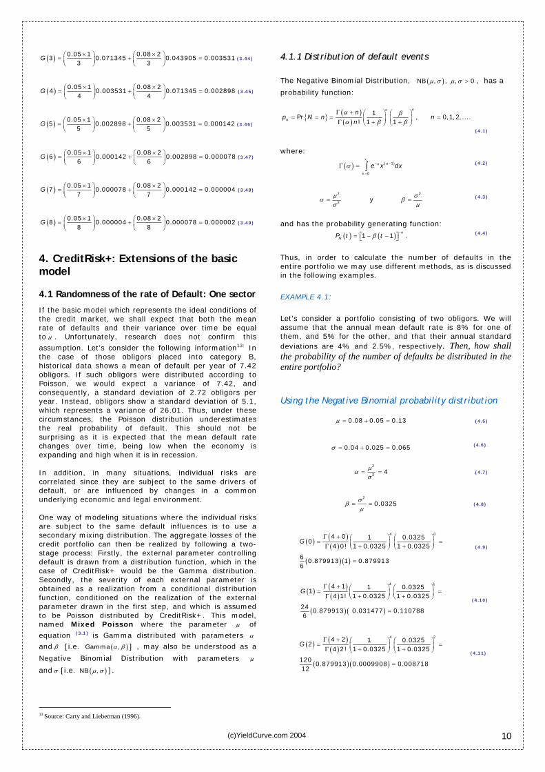
Thus, in order to calculate the number of defaults in the entire portfolio we may use different methods, as is discussed in the following examples. EXAMPLE 4.1:

Let’s consider a portfolio consisting of two obligors. We will assume that the annual mean default rate is 8% for one of them, and 5% for the other, and that their annual standard deviations are 4% and 2.5%, respectively. Then, how shall the probability of the number of defaults be distributed in the entire portfolio? Using the Negative Binomial probability distribution (4.5) 0.08 0.05 0.13µ = + =

0.04 0.025 0.065σ = + = (4.6)

2

2 4µασ

= = (4.7)

2

0.0325σβµ

= = (4.8)

( ) ( )

( )

( ) ( )

4 04 0 1 0.03250

4 0! 1 0.0325 1 0.0325

60.879913 1 0.879913

6

GΓ + ⎛ ⎞ ⎛ ⎞= =⎜ ⎟ ⎜ ⎟Γ + +⎝ ⎠ ⎝ ⎠

=

(4.9)

( ) ( )( )

( ) ( )

4 14 1 1 0.03251

4 1! 1 0.0325 1 0.0325

240.879913 0.031477 0.110788

6

GΓ + ⎛ ⎞ ⎛ ⎞= =⎜ ⎟ ⎜ ⎟Γ + +⎝ ⎠ ⎝ ⎠

=

(4.10)

( ) ( )( )

( ) ( )

4 24 2 1 0.03252

4 2! 1 0.0325 1 0.0325

1200.879913 0.0009908 0.008718

12

GΓ + ⎛ ⎞ ⎛ ⎞= =⎜ ⎟ ⎜ ⎟Γ + +⎝ ⎠ ⎝ ⎠

=

(4.11)

(c)YieldCurve.com 2004 10

( ) ( )( )

( ) ( )

4 34 3 1 0.03253

4 3! 1 0.0325 1 0.0325

7200.879913 0.0000312 0.000549

36

GΓ + ⎛ ⎞ ⎛ ⎞= =⎜ ⎟ ⎜ ⎟Γ + +⎝ ⎠ ⎝ ⎠

=

(4.12)

( ) ( )( )

( ) ( )

4 44 4 1 0.03254

4 4! 1 0.0325 1 0.0325

50400.879913 0.000001 0.000030

144

GΓ + ⎛ ⎞ ⎛= =⎜ ⎟ ⎜Γ + +⎝ ⎠ ⎝

=

⎞⎟⎠ (4.13)

( ) ( )( )

( ) ( )

4 54 5 1 0.03255

4 5! 1 0.0325 1 0.0325

403200.879913 0.00000003 0.000002

720

GΓ + ⎛ ⎞ ⎛ ⎞= =⎜ ⎟ ⎜ ⎟Γ + +⎝ ⎠ ⎝ ⎠

=

(4.14)

Using algorithm 2.2.5:

~

f ( )1 1tα

β−

⎡ ⎤− −⎣ ⎦ n f

Real Imaginary Real Imaginary ( )G n

0 0 1.000000 - 1.000000 - 0.879913

1 1.000000 0.707107 (0.707107) 0.957833 (0.087444) 0.110788

2 0 - (1.000000) 0.871225 (0.110241) 0.008718

3 0 (0.707107) (0.707107) 0.801933 (0.070008) 0.000549

4 0 (1.000000) - 0.777323 - 0.000030

5 0 (0.707107) 0.707107 0.801933 0.070008 0.000002

6 0 - 1.000000 0.871225 0.110241 0.000000

7 0 0.707107 0.707107 0.957833 0.087444 0.000000

Table V Using formulae (55) CreditRisk+ Technical Document ( ) 1

F where 1 1

pt

pt

αβ

pβ

⎛ ⎞ ⎛−= ⎜ ⎟ ⎜− +⎝ ⎠ ⎝

⎞= ⎟

⎠ (4.15)

( )

441 0.031477

F 0 =0.968523 =0.879913 1 0.031477 .

0.0325where

1 0.0325

t

p

−⎛ ⎞= ⎜ ⎟−⎝ ⎠⎛ ⎞= ⎜ ⎟+⎝ ⎠

(4.16)

( )

( )

4

0

42

5

1 0.0314771 0.031477 .

11!

3.4621278.10 173106390.110788

156250000500000000 -157385.

t

ddt t

F

t

=

−⎛ ⎞⎜ ⎟−⎝ ⎠

= =

= =

(4.17)

( )

( )

2 4

0

50

67 8

1 0.0314771 0.031477 .

F 2 =2!

2.724434633.10

1.57385 .10 5.10 0.0174360.008718

2! 2

t

ddt t

t

=

−⎛ ⎞ ⎛ ⎞⎜ ⎟ ⎜ ⎟−⎝ ⎠ ⎝ ⎠

=

−= =

(4.18)

( )

( )

3 4

0

74

711 9

1 0.0314771 0.031477 .

F 3 =3!

3.293069574.10

10 3.1477 .10 0.0032930.000549

3! 6

t

ddt t

t

=

−⎛ ⎞ ⎛ ⎞⎜ ⎟ ⎜ ⎟−⎝ ⎠ ⎝ ⎠

=

−= =

(4.19)

( )

( )

4 4

0

84

89 11

1 0.0314771 0.031477 .

F 4 =4!

7.255916008.10

3.1477 .10 10 0.0007250.000030

4! 24

t

ddt t

t

=

−⎛ ⎞ ⎛ ⎞⎜ ⎟ ⎜ ⎟−⎝ ⎠ ⎝ ⎠

=

−= =

(4.20)

( )

( )

5 4

0

95

911 9

1 0.0314771 0.031477 .

F 5 =5!

1.827155604.10

10 3.1477 .10 0.0001830.000002

5! 120

t

ddt t

t

=

−⎛ ⎞ ⎛ ⎞⎜ ⎟ ⎜ ⎟−⎝ ⎠ ⎝ ⎠

=

−= =

(4.21)

Using the following Panjer14 recursive algorithm: { } { }Pr Pr 1 , 1,2,3,....

bN k a N k k

k⎛ ⎞= = + = − =⎜ ⎟⎝ ⎠

(4.22)

where:

1a

ββ

=+

(4.23)

( )1

1b

α ββ

−=

+ (4.24)

in order to calculate α we use (4.7); (4.8) is used to calculate

β , and (4.15) is used for calculating . { }Pr 0N =

{ }4

4

1 0.031476998Pr 0

1 0.031476998 .0

0.968523 0.879913

N−⎛ ⎞= = =⎜ −⎝

=

⎟⎠ (4.25)

{ } 0.094431Pr 1 0.031477 0.879913 0.110788

1N ⎛ ⎞= = + =⎜ ⎟

⎝ ⎠ (4.26)

{ } 0.094431

Pr 2 0.031477 0.110788 0.0087182

N ⎛ ⎞= = + =⎜ ⎟⎝ ⎠

(4.27)

{ } 0.094431

Pr 3 0.031477 0.008718 0.0005493

N ⎛ ⎞= = + =⎜ ⎟⎝ ⎠

(4.28)

{ } 0.094431

Pr 4 0.031477 0.000549 0.0000304

N ⎛ ⎞= = + =⎜ ⎟⎝ ⎠

(4.29)

{ } 0.094431

Pr 5 0.031477 0.000030 0.0000025

N ⎛ ⎞= = + =⎜ ⎟⎝ ⎠

(4.30)

(c)YieldCurve.com 2004 11

14 Panjer, H. H., “Recursive Evaluation of a Family of Compound Distributions,” ASTIN Bulletin 12, 1981, pp. 22–26.

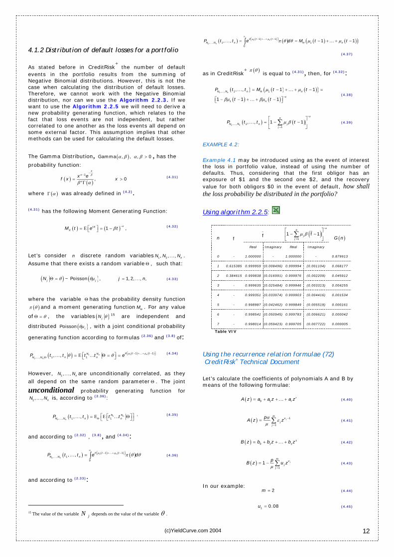
44..11..22 DDiissttrriibbuuttiioonn ooff ddeeffaauulltt lloosssseess ffoorr aa ppoorrttffoolliioo As stated before in CreditRisk

+ the number of default

events in the portfolio results from the summing of Negative Binomial distributions. However, this is not the case when calculating the distribution of default losses. Therefore, we cannot work with the Negative Binomial distribution, nor can we use the Algorithm 2.2.3. If we want to use the Algorithm 2.2.5 we will need to derive a new probability generating function, which relates to the fact that loss events are not independent, but rather correlated to one another as the loss events all depend on some external factor. This assumption implies that other methods can be used for calculating the default losses.

The Gamma Distribution, , has the

probability function:

( )Gamma , , , 0α β α β >

( ) ( )1

, 0

x

x ef x x

α β

αβ α

−−

=Γ

> (4.31)

where ( )αΓ was already defined in (4.2). (4.31) has the following Moment Generating Function:

( ) ( )1 ,tX

XM t e tαβ −⎡ ⎤= Ε = −⎣ ⎦

(4.32)

Let’s consider n discrete random variables .

Assume that there exists a random variable , such that: 1 2, ,..., nN N N

Θ

( ) ( )~ Poisson , 1,2,..., ,j jN jθ θµΘ = = n (4.33)

where the variable Θ has the probability density function

( )π θ and a moment generating function . For any value

of

MΘ

θΘ = , the variables ( )jN θ 15 are independent and

distributed ( )Poisson jθµ , with a joint conditional probability

generating function according to formulas (2.36) and (3.8) of: ( ) ( ) ( )11

1

1 ... 11 1,..., ,..., ... nn

n

t tN Nn nN NP t t t t eθ µ µθ θ ⎡ ⎤− + + −⎣ ⎦

Θ⎡ ⎤= Ε Θ = =⎣ ⎦ (4.34)

However, are unconditionally correlated, as they

all depend on the same random parameter Θ . The joint unconditional probability generating function for

is, according to

1,..., nN N

1,..., nN N (2.36): ( ) 1

1,..., 1 1,..., ... n

n

N NN N n nP t t t tΘ

⎡ ⎤⎡ ⎤= Ε Ε Θ⎣ ⎦⎣ ⎦ , (4.35)

and according to (2.32) , (3.8), and (4.34): ( ) ( ) ( ) ( )1

1

1 ... 1,..., 1

0

,..., n

n

t tN N nP t t e dθ µ µ π θ θ

∞⎡ ⎤− + + −⎣ ⎦= ∫ (4.36)

and according to (2.33):

15 The value of the variable jN depends on the value of the variable θ .

( ) ( ) ( ) ( ) ( ) ( )( )1

1

1 ... 1,..., 1 1

0

,..., 1 ... 1n

n

t tN N n nP t t e d M t tθ µ µ π θ θ µ µ

∞⎡ ⎤− + + −⎣ ⎦

Θ= = − +∫ + −

(4.37)

as in CreditRisk

+ ( )π θ is equal to (4.31), then, for (4.32):

( ) ( ) ( )( )( ) ( )

1,..., 1 1

1

,..., 1 ... 1

1 1 ... 1

nN N n n

n

P t t M t t

t tα

µ µ

βµ βµ

Θ

−

= − + + − =

⎡ ⎤− − + + −⎣ ⎦ (4.38)

( ) ( )

1,..., 11

,..., 1 1n

n

N N n jj

P t t tα

µ β−

=

⎡ ⎤= − −⎢ ⎥

⎣ ⎦∑ (4.39)

EXAMPLE 4.2:

Example 4.1 may be introduced using as the event of interest the loss in portfolio value, instead of using the number of defaults. Thus, considering that the first obligor has an exposure of $1 and the second one $2, and the recovery value for both obligors $0 in the event of default, how shall the loss probability be distributed in the portfolio? Using algorithm 2.2.5:

~

f ( )1

1 f 1n

jj

α

µ β−

=

⎡ ⎤− −⎢ ⎥

⎣ ⎦∑

n f

Real Imaginary Real Imaginary

( )G n

0 - 1.000000 - 1.000000 - 0.879913

1 0.615385 0.999959 (0.008496) 0.999994 (0.001104) 0.068177

2 0.384615 0.999838 (0.016991) 0.999976 (0.002209) 0.045912

3 - 0.999635 (0.025484) 0.999946 (0.003313) 0.004255

4 - 0.999351 (0.033974) 0.999903 (0.004416) 0.001534

5 - 0.998987 (0.042462) 0.999849 (0.005519) 0.000161

6 - 0.998541 (0.050945) 0.999783 (0.006621) 0.000042

7 - 0.998014 (0.059423) 0.999705 (0.007722) 0.000005

Table VIV

Using the recurrence relation formulae (72) CreditRisk+ Technical Document Let’s calculate the coefficients of polynomials A and B by means of the following formulae:

(4.40)( ) 0 1 ... r

rA z a a z a z= + + +

( ) 1

1

jm

vj

j

pA z z

α εµ

−

=

= ∑ (4.41)

(4.42)( ) 0 1 ... s

sB z b b z b z= + + +

( )

1

1 jm

vj

j

pB z u z

µ =

= − ∑ (4.43)

In our example: 2m = (4.44)

(c)YieldCurve.com 2004 12

(4.45)1 0.08u =

(4.46)2 0.05u =

(4.47)1 2 0.08 0.05 0.13µ µ µ= + = + =

(4.48)1 2 0.04 0.025 0.065σ σ σ= + = + =

2 2

2 2

0.134

0.065µασ

= = = (4.49)

2 20.0650.0325

0.13σβµ

= = = (4.50)

( )0.0325

0.031476997571 1 0.0325

pβ

β= = =

+ + (4.51)

(4.52)1 1v =

2 2v = (4.53)

1 1 (4.54)1 0.08vε µ= =

(4.55)2 2 2 0.10vε µ= =

( ) ( 00.03147699757 4

0.08 0.10 ,0.13

A z z z×

= + )1 (4.56)

(4.57)( ) 0.07748184019+0.09685230024A z z=

( ) ( )1 20.03147699757

1 0.080.13

B z z z= − + 0.05 (4.58)

(4.59)( ) 2 1- 0.01937046004 - 0.01210653753B z z z=

(4.60)1r =

2s = (4.61)

Now, we have the coefficients of each polynomial:

(4.62)0 10.07748184019, 0.09685230024a a= =

(4.63)0 1 21, 0.01937046004, 0.01210653753b b b= = − = −

Having calculated the coefficients, it is possible to use formula (72) of the CreditRisk+ technical document to calculate the loss distribution from . Consequently, it is necessary to calculate the loss for first by using

formula (59) of the CreditRisk

1A

0A+

technical document or formula (4.15) of this paper:

( )( )

( )( )

4

0

4

1 1 0.03147699757

1 0 1 0.03147699757 0

0.96852300 0.879913

pA

p

α⎡ ⎤ ⎡− −

= =⎢ ⎥ ⎢− × − ×⎢ ⎥ ⎢⎣ ⎦ ⎣

= =

⎤⎥⎥⎦ (4.64)

( ) ( )( )( )min , min 1, 1

1 10 00

11

r n s n

n i n i j n ji j

A a A b nb n

− −

+ − += =

⎛= −⎜⎜ ⎟+ ⎝

∑ ∑ j A −

⎞− ⎟

⎠ (4.65)

(4.66)( ) ( )1 0.07748184 0.879913 0.068177A = × =

( )( )( )0.07748184 0.068177+0.0968523 0.8799131

2 ,2 0.01937046 0.068177

⎡ ⎤× × −= ⎢ ⎥

− ×⎢ ⎥⎣ ⎦A

(4.67)

(4.68)( )2 0.045912A =

(

)

( )045912+0.0968523 0.068177

0.045912 0.01210653753 0.068177

0.07748184 0.1(3)

3 0.01937046 2A

⎡ ⎤× × −= ⎢ ⎥

× − ×− ×⎢ ⎥⎣ ⎦

(4.69)

(4.70)( )3 0.004255A =

( )( )( )0.07748184 0.004255+0.0968523 0.0459121

44 0.01937046 3 0.004255 0.01210653753 2 0.045912

A⎡ ⎤× × −

= ⎢ ⎥− × × − × ×⎢ ⎥⎣ ⎦

(4.71)

(4.72)(4) 0.001534A =

( )

( )( )0.07748184 0.001534+0.0968523 0.0042551

55 0.01937046 4 0.001534 0.01210653753 3 0.004255

A⎡ ⎤× × −

= ⎢ ⎥− × × − × ×⎢ ⎥⎣ ⎦

(4.73)

(4.74)( )5 0.000161A =

( )

( )( )0.07748184 0.000161+0.0968523 0.0015341

66 0.01937046 5 0.000161 0.01210653753 4 0.001534

A⎡ ⎤× × −

= ⎢ ⎥− × × − × ×⎢ ⎥⎣ ⎦

(4.75)

(4.76)( )6 0.000042A =

( )

( )( )0.07748184 0.000042+0.0968523 0.0001611

77 0.01937046 6 0.000042 0.01210653753 5 0.000161

A⎡ ⎤× × −

= ⎢ ⎥− × × − × ×⎢ ⎥⎣ ⎦

(4.77)

(4.78)( )7 0.000005A =

Using the Panger16 recursive algorithm This algorithm was already discussed when we calculated the default distribution, but it can also be used (with some minor

adjustments) to assess the loss distribution.17

Suppose that the severity distribution is defined for

0,1,2... so that in this example:

( )Xf x

16 Work quoted in 14

(c)YieldCurve.com 2004 13

17 The same algorithm may be used for the assessment of the distribution of defaults and losses, considering the basic model of CreditRisk+. The only change takes place in

formulas (4.23) and (4.24), where: 0a = and b µ= ; and consequently, the algorithm (4.85) is reduced to algorithm (4.89).

( ) 1 0.081 0.61538462

0.13Xfµµ

= = = (4.79)

( ) 2 0.05

2 0.384615380.13Xf

µµ

= = = (4.80)

Suppose that the frequency distribution is a member of

the ( class and that complies with formula ),a b (4.22). Note

that both the Poisson distribution and the Negative Binomial distribution are included in this class. For example, in the case of the Poisson distribution ( )Poisson µ ,

and b0a = µ= . For the Negative Binomial distribution, i.e. ( ) ,Negative Binomial µ σ , , , and a b α β are calculated using (4.23),(4.24), (4.7) and (4.8) respectively. In our previous

example, these formulas result in the following values:

2

2 4µασ

= = (4.81)

2

0.0325σβµ

= = (4.82)

0.03250.031476998

1 1.0325a

ββ

= = =+

(4.83)

( ) ( )1 4 1 0.03250.09443099

1 1 0.0325b

α ββ

− − ×= = =

+ + (4.84)

Panjer showed that the loss distribution could be

recursively evaluated using:

( )Sf x

( ) ( ) ( )1

x

S X Sy

byf x a f y f x y

x=

⎡ ⎤⎛ ⎞= + −⎢ ⎜ ⎟⎝ ⎠⎣ ⎦

∑ ⎥ (4.85)

The starting value of the recursive algorithm is:

( ) ( )( )4

4

1 1 0.0314769980 0

1 1 0.031476998 .0

0.968523 =0.879913

S N X

af P f

at

α− −⎛ ⎞ ⎛ ⎞= = =⎜ ⎟ ⎜ ⎟− −⎝ ⎠ ⎝ ⎠

= (4.86)

Now we can calculate the other values of ( )Sf x 18:

( ) ( )1 0.031476998 0.09443099 0.61538462 0.879913

0.068177Sf = + × × =

(4.87)

( ) 0.094430992 0.031476998 0.61538462 0.879913

2

0.09443099 20.031476998 0.38461538 0.068177 =0.045912

2

Sf⎡⎛ ⎞= + × × +⎢⎜ ⎟⎝ ⎠⎣

⎡ ×⎛ ⎞+ + × ×⎢⎜ ⎟⎝ ⎠⎣

⎤⎥⎦

⎤⎥⎦

(4.88)

In the case of X~ ( )Poisson µ , (4.85) is reduced to: ( ) ( ) ( )

1

, 1,2,...,x

S X Sy

f x yf y f x y xxµ

=

= − =∑ (4.89)

18 Here, we are only calculating the values for 0,1, 2.=X

4.2 Several Sectors Once the assumptions for the randomness of the default rate have been made, CreditRisk

+ next focuses on the decomposition of the default rate by sectors. In practical

terms:19

1

m

ik kk

aµ µ=

= ∑ ε (4.90)

where kε is a Gamma distributed random variable, and which

represents the k factor, with a mean equal to one and a standard deviation represented by , and with being m the

total number of factors. The sum of the weights of the factors in the determination of the mean shall be 1:

ks

ika

(4.91)1

1 for all m

ikk

a=

=∑ i

ika

When approaching the calculation of the loss distribution using this framework for several sectors we could use Monte

Carlo simulation20. Although this approach adapts to any probability distribution, both for modeling the uncertainty in the factor and uncertainty in the loss distribution, it is generally an inefficient means for computation due its computing resource requirements. Another methodology is the one used by Finger21, and is similar to the approach that will be taken later in this paper. It combines Monte Carlo Simulation for modeling factor uncertainty (using standard normal distribution), and the FFT for modeling the loss distribution in a portfolio (assuming a Binomial distribution in this case). Despite the fact that this methodology chooses the probability distributions for us, which can be an advantage, the problems with Monte Carlo simulation persist. Last, but not least, CreditRisk+ uses the Gamma and the Poisson distributions as mentioned in the previous sections. This is a clear advantage as these distributions allow us to maintain a recurrence relation, which is quite effective in computing terms. Here the disadvantage is that there is no convincing research22 which proves the uncertainty surrounding the

default probability follows a Gamma distribution. We shall now introduce the Value at Risk calculation for a credit portfolio using the distributions assumed by

CreditRisk+, but instead using the FFT.

44..11..22 LLoossss DDiissttrriibbuuttiioonn uussiinngg FFFFTT Each sector is considered a portfolio by itself, and completely independent from the other sectors. The portfolio is thus partitioned into as many sub portfolios as there are sectors. Each sector portfolio will be assigned a weight

corresponding to its idiosyncratic risk23, and which is in accordance with the concept proposed by William F. Sharpe; that is to say, the portion of the default rate that is not accounted for by systemic factors, sectors, etc., but by the financial structure of the obligor or itself. In this sub portfolio

19 Reconciling CreditRisk+ and CreditMetrics by Li,Song and Ong. 20 A comparative anatomy of credit risk models by Michael Gordy. 21 See note 822 See note 9

(c)YieldCurve.com 2004 14

23 It can also be called Idiosincratic Risk or own Risk.

(following the CreditRisk+

Technical Document section A

12.3) the losses are distributed Poisson. In the other sub portfolios, however, losses are distributed according to the extended model. Once the loss distribution for each sub portfolio is calculated, it is then possible to calculate the loss distribution for the entire portfolio using algorithm 2.2.3, as each sub portfolio is independent from the others. This is clearly shown in the following example: EXAMPLE 4.3 24

Let’s continue with our real world containing only two obligors. One of them is an issuer with a bond priced at $1, having a default probability of 16% and a standard deviation of 8%. The other one is an obligor with an outstanding loan of $2, with a default probability of 10% and a standard deviation of 5%. In both cases, the recovery value at default is $0. We have seen this kind of data in previous examples; however, in this case it is necessary to add up the weights of each sector when determining the mean default of each obligor. The following table introduces the required information:

Obligor / Issuer Sector A Sector B

1 0.50 0.50

2 0.50 0.50

Table VII

First, we shall partition the portfolio by the number of sectors chosen. Thus, we find out in our example that we have two new portfolios, namely:

Portfolio A

Obligor/ Issuer

Exposure $ µ σ ika ikaµ µ= ikaσ σ=

1 1 0.16 0.08 0.50 0.08 0.04 2 2 0.10 0.10 0.50 0.05 0.025

Table VIII

Portfolio B Obligor/ Issuer

Exposure $ µ σ ika ikaµ µ= ikaσ σ=

1 1 0.16 0.08 0.50 0.08 0.04 2 2 0.10 0.10 0.50 0.05 0.025

Table IX

We next calculate the loss distribution of each new portfolio by means of the algorithm 2.2.3. Formula (72)

of the CreditRisk+ technical document may be used to

calculate the loss distribution of the entire portfolio, as will be discussed later. As for the values in this example, both distributions happen to be equal. The calculations to be carried out for their determination are also equal to the ones described in previous sections. 24 The values in this example were chosen in such a way that calculations made in the prevIous examples may be used in this one.

Loss Distribution

Portfolio A Portfolio B

0.879913 0.879913

0.068177 0.068177

0.045912 0.045912

0.004255 0.004255

0.001534 0.001534

0.000161 0.000161

0.000042 0.000042

0.000005 0.000005

Table X

Let’s now use algorithm 2.2.3 for determining the loss distribution for the whole portfolio:

Using algorithm 2.2.3:

~

f

~

g ~

h n ( )G nf g

Real Imaginary Real Imaginary Real Imaginary

0 0.879913 0.879913 1.000000 - 1.000000 - 1.000000 - 0.774247

1 0.068177 0.068177 0.976897 (0.064200) 0.976897 (0.064200) 0.950206 (0.125434) 0.119980

2 0.045912 0.045912 0.923470 (0.096971) 0.923470 (0.096971) 0.843393 (0.179099) 0.085446

3 0.004255 0.004255 0.869783 (0.092263) 0.869783 (0.092263) 0.748010 (0.160497) 0.013748

4 0.001534 0.001534 0.835494 (0.064079) 0.835494 (0.064079) 0.693944 (0.107075) 0.005387

5 0.000161 0.000161 0.825171 (0.030341) 0.825171 (0.030341) 0.679986 (0.050074) 0.000883

6 0.000042 0.000042 0.833291 (0.005230) 0.833291 (0.005230) 0.694346 (0.008716) 0.000254

7 0.000005 0.000005 0.847798 0.003857 0.847798 0.003857 0.718746 0.006539 0.000042

8 0.000001 0.000001 0.854804 - 0.854804 - 0.730690 - 0.000010

9 0.000000 0.000000 0.847798 (0.003857) 0.847798 (0.003857) 0.718746 (0.006539) 0.000002

10 0.000000 0.000000 0.833291 0.005230 0.833291 0.005230 0.694346 0.008716 0.000000

11 0.000000 0.000000 0.825171 0.030341 0.825171 0.030341 0.679986 0.050074 0.000000

12 0.000000 0.000000 0.835494 0.064079 0.835494 0.064079 0.693944 0.107075 0.000000

13 - - 0.869783 0.092263 0.869783 0.092263 0.748010 0.160497 0.000000

14 - - 0.923470 0.096971 0.923470 0.096971 0.843393 0.179099 0.000000

15 - - 0.976897 0.064200 0.976897 0.064200 0.950206 0.125434 -

Table XI

Using the recurrence relation formulae (72) of the CreditRisk+ Technical Document As the algorithm was already explained in the previous section, here we only focus on the sectors and the calculation of the three first values of for each. Once again, the values used in this example make the calculation easier. The following formulas calculate the probability generating

function of 0 as a product of (4.64): (4.92)0 0.879913 0.879913 0.774247A = × =

In order to evaluate the polynomials zA and zB we proceed as

follows:

(c)YieldCurve.com 2004 15

( )( )

( )( )

( ) ( )( )

( ) ( )( )

( ) ( )( )

1 2

1 2

1 21 1211 1 2 2

1 11 21 2

1 21 2

1 11 2

1 1

j j

j j

m mv v

j jj j

m mv v

j jj j

p pz z

A z

B z p pu z u z

α αε ε

µ µ

µ µ

− −

= =

= =

= +− −

∑ ∑

∑ ∑ (4.93)

in our example:

( )( )

( ) ( )( )1 21 2

1 1211 1 2 2

1 11 2

j

m mv v

j jj j

p pz z

α αε ε

µ µ− −

= =

=∑ ∑ j (4.94)

( ) ( )( )( ) ( )( )1 21 2

1 21 2

1 11 2

1 1j

m mv v

jj j

p pu z u z

µ µ= =

− = −∑ ∑ j

j (4.95)

therefore:

( )( )

1

1

1

2

1

j

j

mv

jj

mv

jj

pz

A zpB z z

α εµ

µµ

−

=

=

⎛ ⎞×⎜ ⎟

⎝ ⎠=−

∑

∑ (4.96)

For (4.57): ( ) ( )0.07748184019+0.09685230024 2

0.1549636803 0.1937046004

A z z

z

= ×

+

= (4.97)

For (4.59): (4.98)( ) 2 1- 0.01937046004 - 0.01210653753B z z z=

(4.99)0 10.1549636803, 0.1937046004a a= =

(4.100)0 1 21, 0.01937046004, 0.01210653753b b b= = − = −

(4.101)( ) ( )1 0.1549636803 0.774247 0.119980A = × =

( ) ( ) (12 0.15496 0.11998+0.19370 0.7742 0.01937 0.11998

2A ⎡ ⎤= × × − − ×⎣ ⎦)

(4.102)

(4.103) 2 0.085446A =

5. CreditRisk+ by FFT In this section, we introduce a fully developed example for calculating the Value at Risk of a given credit portfolio. Likewise, and with the aim of bridging the gap between theory and computerized application, we introduce the examples using MatLab, R and VBA. Before we proceed, it is vital to review some of the basic concepts used by

CreditRisk+, namely:

Exposure:

Exposure is defined as the net loss suffered by the creditor if his counterparty fails to pay. In other words, it is the expected recovery amount at default. So, in order to calculate the LGD (Loss Given Default) it is necessary to know beforehand the recovery amount. Bands:

The amounts into which a portfolio is subdivided. Each band is considered an independent portfolio.

EXAMPLE 5.1 25

Suppose the bank holds a portfolio of loans and bonds across 500 different obligors, with exposures ranging between

$50,000 and $1 million:

Notation

Obligor Exposure Probability of Default Expected Losses

A

AL

AP

x A A AL Pλ =

In the following table, we introduce the first six obligors:

Obligor

A

Exposure

AL Exposure in $100.000

Exposure in $100.000

jv

Band

j

1 150.000 1.5 2 2 2 460.000 4.6 5 5 3 435.000 4.35 5 5 4 370.000 3.7 4 4 5 190.000 1.9 2 2 6 480.000 4.8 5 5

The exposure unit . Each band with

has a mean ordinary exposure valuev j

$100.000L = , 1,2,...,j j m=

10m = . $100.000j = ×

In CreditRisk+ each band is considered an independent portfolio of loans and/or bonds. Thus:

Notation

Ordinary exposure in band by units of j L

Expected loss in band by units of j L

Expected number of defaults in band j

jv

jε

jµ

Then, by definition, we get:

j j jvε µ= × (5.1)

Whence:

jj

jv

εµ = (5.2)

Indicated by Aε , the expected loss for obligor in units of ,

for example, is:

A L

AA L

λε = (5.3)

Then, the annual expected loss in band , jj ε , expressed in

units of L , is simply the sum of the expected loss Aε for all

obligors that belong to band . For instance: j

: A j

j AA v v

ε ε=

= ∑ (5.4)

From (5.2) it follows that the expected number of annual defaults in band is: j

: :A j A j

j Aj

A v v A v v

A

j j Av v

εv

ε εµ

= =

= = =∑ ∑ (5.5)

25 This same example was been introduced in the work quoted in note 2

(c)YieldCurve.com 2004 16

The following table illustrates the possible outcomes when performing the calculations:

Band j Number of

obligors jε jµ

1 30 1.5 1.5 2 40 8 4 3 50 6 2 4 70 25.2 6.3 5 100 35 7 6 60 14.4 2.4 7 50 38.5 5.5 8 40 19.2 2.4 9 40 25.2 2.8 10 20 4 0.4

5.1 Basic Model of CreditRisk+:

5.1.1 Basic Model Algorithm by FFT

Having fleshed out the algorithm introduced in section 2.2.3, we can now describe the calculations for the loss distribution of the whole portfolio using FFT as per the following instructions:

1. We choose dimension of the probability vector , being especially mindful of the remarks

mentioned in the last three paragraphs of section 2.2.3

nf

26 2. We build a probability vector for each band j 27,

such that:

( ) defaults !

for 0,1,2,...,2 y 1,2,...,

jnj

r

eP n

nn j

µµ −

=

= = m

(5.6)

3. We derive the loss distribution vector in the portfolio by means of the following formula:

(5.7)( )

1

IFFT FFT fm

jj =

⎧ ⎫⎪ ⎪⎨ ⎬⎪ ⎪⎩ ⎭∏

At first glance, this algorithm looks somehow different than the one introduced in section 2.2.3. However, it is quite simple to explain the differences. In algorithm 2.2.3, we assigned a vector for each obligor (i.e. f and ). Here, following the same criteria, we shall use as

many vectors as there are obligors in band j, and recognizing that the probability of default for a particular band is the same for all the obligors contained in that

band, we have

g

nº of obligors in band j

j

µ.

It is possible to simplify the calculation using a single probability vector, computing the FFT of such vector and afterwards, using the power of complex numbers to raise the vector up to an exponent equal to the number of obligors that comprise the band. Simplifications, however, do not stop here. It turns out that when using algorithm 2.2.3 it is also possible to delete said power if using the expected number of defaults in band , jj µ , instead of the

probability of default . AP

26 In our example, the portfolio is 2.630 units of L and the expected loss 177; the unexpected loss is hardly higher than 1024, which is to say 210. This is a suitable value for n, then. 27 Although we asume a Poisson distribuition for defaults, as in CreditRisk+, it is also possible to choose a binomial distribution.

5.2 Extended Model of CreditRisk+: 55..22..11 OOnnee SSeeccttoorr 5.2.1.1 Extended Model Algorithm, One Sector by FFT As mentioned in section 4, in the real world the mean rate of defaults, as well as the variance of defaults, changes over time. Consequently, the previous algorithm may underestimate the credit risk of the portfolio. In order to solve

this problem, CreditRisk+ introduces an alternative to the

basic model, using Poisson to develop the process of default, but assuming that the mean rate is stochastic with mean

and standard deviationAP

APσ . To model this uncertainty,

CreditRisk+ adopts the Gamma distribution, and assumes a

mean of one and a standard deviation equal to . In our example, , so let us now calculate the loss distribution for the whole portfolio using the

s

0.50s =

algorithm 2.2.5:

1. Calculate the parameters α , β and s:

AP

A

sP

σ=

28

2

2

1 =

1s

sα β=

(5.8)

2. We build a severity vector, such that:

( )

0

f for 1,2,3,...,jm

ii

j jµ

µ=

= =

∑m

(5.9)

3. We calculate the FFT of said vector:

(5.10) ( )

~

f =FFT f

4. Apply the probability generating function, element by

element, to the FFT of the severity vector:

~ ~

Z

1

f 1 f 1m

jj

α

µ β−

=

⎡ ⎤⎛ ⎞ ⎛ ⎞= − −⎢ ⎥⎜ ⎟ ⎜ ⎟⎝ ⎠⎢ ⎥⎝ ⎠⎣ ⎦

∑ (5.11)

5. Apply the IFFT to recover the distribution of

Cumulative losses:

~

Z Zf =IFFT f⎛ ⎞⎜ ⎟⎝ ⎠

(5.12)

When tends to zero the result from the prior algorithm matches the result of algorithm 5.1.1, so both can be used

for calculating the loss distribution in the basic CreditRisk

s

+

model. Moreover, this last feature shall be vital when the random rate of default depends upon factors external to the obligor, as we shall see in the next section. 55..22..22 SSeevveerraall SSeeccttoorrss

28 In order to delve deeply into this subject, we suggest the paper already quoted in note 19 page 8, where from the following reference is quoted: “Strictly speaking, this means that CreditRisk+ requires that the ratio

AP

APσ

(c)YieldCurve.com 2004 17

shall be the same for all debtors asociated with the same sector”.

In this case (as already discussed in section 4), it is necessary to create additional sector allocations for each obligor as the below table shows:

Band

jNº of

Obligors jε jµ Own Risk

Sector A

Sector B Total

1 30 1.5 1.5 50% 25% 25% 100% 2 40 8 4 50% 25% 25% 100% 3 50 6 2 50% 25% 25% 100% 4 70 25.2 6.3 50% 25% 25% 100% 5 100 35 7 50% 50% 0% 100% 6 60 14.4 2.4 50% 50% 0% 100% 7 50 38.5 5.5 50% 50% 0% 100% 8 40 19.2 2.4 50% 50% 0% 100% 9 40 25.2 2.8 50% 50% 0% 100% 10 20 4 0.4 50% 50% 0% 100%

Here we have added up the percentage participations of the various sectors involved in determining the stochastic default rate. With the aim of developing a complete example, we have also incorporated a “special” sector called “own risk”29 (following William F. Sharpe’s criteria), which represents the portion of the rate of default that is not accounted for by systematic movements of the sectors, but by the particular financial structure of the issuer or obligor. Before developing this algorithm, it is worth mentioning that each sector is assumed to be an independent portfolio, and is in keeping with the

CreditRisk+ criteria. Thus, the portfolio in this example can

be broken down into three sub portfolios of which one is detailed in the following table:

Sub-Portfolio 1

Band

j Nº of Obligors Own Riskjε × jµ

1 30 0.75 0.75 2 40 4 2 3 50 3 1 4 70 12.6 3.15 5 100 17.5 3.5 6 60 7.2 1.2 7 50 19.25 2.75 8 40 9.6 1.2 9 40 12.6 1.4 10 20 2 0.2

If part of the default rate can be explained by the idiosyncratic risk of the obligors in the portfolio, then following steps are to be taken to calculate the loss distribution for the whole portfolio:

5.2.2.1 Algorithm extended model several sectors by FFT

1. Use algorithm 5.2.1.1 as many times as there are sub portfolios. Let s be a value very close to zero30 when calculating the loss distribution of the sub portfolio’s idiosyncratic risk, and use a value greater than zero31 for the remaining sectors. From this step we obtain as many loss distribution vectors as there are sub portfolios.

2. Apply algorithm 2.2.3 in order to recover the

probability vector as a convolution of the loss distribution vectors obtained in the prior step.

29 It is also referred to as idiosyncratic or specific risk.

30 APσ=0.0001 gets correct results

31 We use s=0.50 because CreditRisk+ makes use of that value.

6. Conclusions

We have introduced an alternative way of calculating credit

Value at Risk using CreditRisk+. This alternative, which

resorts to the Fast Fourier Transform (FFT), may be used not only for supporting the calculations of the original implementation of CreditRisk+ (following Gordy32’s suggestions), but also for generally calculating the loss distribution of any credit portfolio. Moreover, the methodology developed in this paper does not limit its

application to CreditRisk+, as it can be in conjunction with

Monte Carlo Simulation for modeling credit risk, as suggested

by Finger33.

7. References

CreditMetrics™ -- Technical Document April 2, 1997 by Greg M. Gupton of the Morgan Guaranty Trust Company, Christopher C. Finger of the Morgan Guaranty Trust Company, and Mickey Bhatia of the Morgan Guaranty Trust Company Modeling Default Risk Modeling Default Risk December 18, 2003 by Peter J. Crosbie of Moody's|KMV, and Jeffrey R. Bohn of Moody's|KMV CreditRisk+ A Credit Risk Management Framework

Credit Suisse First Boston. Credit Risk+. Technical document,

Credit Suisse First Boston October 1997 by Tom Wilde of CSFB A Comparative Analysis of Current Credit Risk Models February 2000 by Michel Crouhy of the Canadian Imperial Bank of Commerce, Dan Galai of the Hebrew University, and Robert Mark of the Canadian Imperial Bank of Commerce Sticks and stones. Working Paper, RiskMetrics Group. October 1998 by Christopher C. Finger (Free logon required ) A Comparative Anatomy of Credit Risk Models December 8, 1998, by Michael B. Gordy of the Board of Governors of the Federal Reserve System Portfolio Credit Risk I. Risk, September 1997 by Wilson, T. Portfolio Credit Risk II. Risk, October 1997 by Wilson, T. Conditional approaches for credit metrics portfolio distributions. April 1999 Credit Metrics Monitor 2(1):14–33. by Christopher C. Finger ( Free logon required ) A Generalized Framework for Credit Risk Portfolio Models September 14, 1998 by H. Ugur Koyluoglu of Oliver, Wyman & Company, and Andrew Hickman of CSFP Capital, Inc. Integrating Correlations July 1999

32 Publication quoted in 9

(c)YieldCurve.com 2004 18

33 Publication quoted in 8

(c)YieldCurve.com 2004 19

by Peter Bürgisser of the Universität Paterborn, Alexandre Kurth of the Universität Basel, Armin Wagner of UBS, and Michael Wolf of UBS Aggregation of Correlated Risk Portfolios: Models & Algorithms, CAS Committee on Theory of Risk. Working Paper. 1999 by WANG, S. S Reconciling CreditRisk+ and CreditMetrics, by Li, Song and Ong. Recursive Evaluation of a Family of Compound Distributions ASTIN Bulletin 12, 1981, pp. 22–26, by Panjer, H. H. Saddlepoint Approximation of CreditRisk+ August 2002 Published in Journal of Banking and Finance, 26(7), pp. 1337-1355. by Michael B. Gordy of the Board of Governors of the Federal Reserve System