
CreditRisikDefaultModelsCreditDerivatives
192
Credit Risk, Default Models and Credit Derivatives Master of Finance, Special Course WS 2011 Prof. Dr. Wolfgang M. Schmidt Frankfurt School of Finance & Management September/October 2011 – Typeset by Foil T E X –
Transcript of CreditRisikDefaultModelsCreditDerivatives

Credit Risk, Default Models and Credit DerivativesMaster of Finance, Special Course WS 2011
Prof. Dr. Wolfgang M. Schmidt
Frankfurt School of Finance & Management
September/October 2011
– Typeset by FoilTEX –

AbstractThe course provides an introduction to the modeling and management of credit risk.
Main emphasis of the course are default models that are used in banking practice in the
fields of risk management and credit derivatives.
The first part of the course deals with credit derivatives. To understand the market for
credit derivatives, a comprehensive examination of credit default swaps is indispensable.
We investigate further important types of credit derivative products, such as, for example,
credit indices, basket default swaps or CDOs, including their modeling and valuation.
In the second part we extend the analysis of risk as covered in the core course on
risk management by investigating credit risk management in more depth. We study the
rationale behind the new Basel II accord concerning credit risk as well as industry standard
models for portfolio credit risk.
Recommended further reading are [Blum et al., 2003], [Duffie and Singleton, 2003],
[Lando, 2004], [Saunders and Allen, 2002]. For a comprehensive source on all aspects of
risk management we refer to [Jorion, 2009].
– Typeset by FoilTEX – 1
Contents
I Credit Derivatives 9
1 Introduction to credit derivatives: applications, the market and market participants 10
2 The first credit derivative: asset swap 16
3 Credit default swaps 21
3.1 First applications, cash flows and quotation . . . . . . . . . . . . . . . . . . 21
3.2 No-arbitrage relationships . . . . . . . . . . . . . . . . . . . . . . . . . . . 29
3.3 The cash–CDS basis, CDS strategies of market participants . . . . . . . . . . 33
– Typeset by FoilTEX – 2

3.4 Credit linked notes, funded CDS . . . . . . . . . . . . . . . . . . . . . . . . 38
4 Mark-to-market and the CDS curve 40
4.1 Pricing directly from spread differences . . . . . . . . . . . . . . . . . . . . 41
4.2 Deriving the default probabilities from market data . . . . . . . . . . . . . . . 43
4.3 Mark-to-market valuation of credit default swaps . . . . . . . . . . . . . . . . 52
4.4 How critical are the assumptions on the recovery rate? . . . . . . . . . . . . . 53
5 Lessons from the credit crisis 55
5.1 Issues highlighted by the crisis . . . . . . . . . . . . . . . . . . . . . . . . 55
5.2 Private sectors initiatives . . . . . . . . . . . . . . . . . . . . . . . . . . . 59
– Typeset by FoilTEX – 3

6 Strategies with CDS 62
6.1 Funding cost strategies . . . . . . . . . . . . . . . . . . . . . . . . . . . . 62
6.2 Curve trades . . . . . . . . . . . . . . . . . . . . . . . . . . . . . . . . . 63
6.3 Credit vs equity . . . . . . . . . . . . . . . . . . . . . . . . . . . . . . . . 64
6.4 Sub vs senior . . . . . . . . . . . . . . . . . . . . . . . . . . . . . . . . . 65
7 Default modeling 68
7.1 Default intensity, hazard rate out of today . . . . . . . . . . . . . . . . . . 69
7.2 Models for the default time . . . . . . . . . . . . . . . . . . . . . . . . . . 73
7.2.1 Structural models . . . . . . . . . . . . . . . . . . . . . . . . . . . 74
7.2.2 Reduced form models . . . . . . . . . . . . . . . . . . . . . . . . . 76
– Typeset by FoilTEX – 4

8 CDS Indices 80
9 Correlation products 85
9.1 Basket Default Swaps . . . . . . . . . . . . . . . . . . . . . . . . . . . . . 85
9.2 CDO Tranches . . . . . . . . . . . . . . . . . . . . . . . . . . . . . . . . 89
9.3 Synthetic CDO tranches on the benchmark index . . . . . . . . . . . . . . . 91
10 What is default correlation? 94
10.1 Event correlation . . . . . . . . . . . . . . . . . . . . . . . . . . . . . . . 96
10.2 Asset correlation . . . . . . . . . . . . . . . . . . . . . . . . . . . . . . . 97
11 Monte-Carlo valuation 100
– Typeset by FoilTEX – 5
11.1 How to simulate default times? . . . . . . . . . . . . . . . . . . . . . . . . 101
11.2 How to generate dependent simulations? . . . . . . . . . . . . . . . . . . . 102
11.3 Normal copula and asset correlation . . . . . . . . . . . . . . . . . . . . . . 104
11.4 Pricing basket CDS . . . . . . . . . . . . . . . . . . . . . . . . . . . . . . 107
11.5 Pricing tranches of CDOs . . . . . . . . . . . . . . . . . . . . . . . . . . . 110
II Credit Risk Management 113
12 Credit risk 114
13 Modeling default 117
– Typeset by FoilTEX – 6
14 Credit risk management, credit-value-at-risk and Basel II 122
14.1 Traditional methods of credit risk management . . . . . . . . . . . . . . . . 122
14.2 Traditional approaches to credit risk assessment . . . . . . . . . . . . . . . . 124
14.3 Economic capital . . . . . . . . . . . . . . . . . . . . . . . . . . . . . . . 125
14.4 Portfolio risk - the correlation problem . . . . . . . . . . . . . . . . . . . . . 129
14.5 Regulatory requirements, Basel II . . . . . . . . . . . . . . . . . . . . . . . 133
15 Credit risk management in banks and industry standard models 141
15.1 Estimating default probabilities . . . . . . . . . . . . . . . . . . . . . . . . 141
15.2 The Merton model . . . . . . . . . . . . . . . . . . . . . . . . . . . . . . 146
15.3 The KMV model . . . . . . . . . . . . . . . . . . . . . . . . . . . . . . . 151
– Typeset by FoilTEX – 7

15.3.1 Dependent defaults in the Merton model . . . . . . . . . . . . . . . . 152
15.3.2 1-Factor dependence and the Basel II formula . . . . . . . . . . . . . 156
15.4 CreditMetrics . . . . . . . . . . . . . . . . . . . . . . . . . . . . . . . . . 163
15.5 Credit Risk+ . . . . . . . . . . . . . . . . . . . . . . . . . . . . . . . . . 174
15.6 Comparison KMV/CreditMetrics versus CreditRisk+ . . . . . . . . . . . . . . 184
Prof. Dr. W. M. Schmidt 8 Credit Risk, Master of Finance, Special Course WS 2010

Part I
Credit Derivatives
Prof. Dr. W. M. Schmidt 9 Credit Risk, Master of Finance, Special Course WS 2010

1 Introduction to credit derivatives: applications, the market and market participants
1 Introduction to credit derivatives: applications, the marketand market participants
Credit derivatives allow for a customized and flexible transfer of credit risk independently of some
funding. Traditional credit products such as loans or bonds are restricted in terms of available
conditions, in addition they require an initial investment of capital (funding).
The rationale and economic motivation of market participants to enter into credit derivatives
to take on “positive” or “negative” credit risk exposures can be quite different.
Credit derivatives can be used to
• reduce/hedge credit risk,
• actively take certain credit risks,
• generate extra returns,
• set up tailor made structured credit risk profiles,
Prof. Dr. W. M. Schmidt 10 Credit Risk, Master of Finance, Special Course WS 2010

1 Introduction to credit derivatives: applications, the market and market participants
• generate synthetic bonds/loans that are not available in the market in this form (time to
maturity, currency, etc.).
Credit derivatives play an important role in efficient allocation of risk and capital.
The market size in credit derivatives still continues to grow dramatically every year.
The outstanding volume in credit derivatives nowadays exceeds the volume in equity derivatives
and corporate bond issuance.
Prof. Dr. W. M. Schmidt 11 Credit Risk, Master of Finance, Special Course WS 2010

1 Introduction to credit derivatives: applications, the market and market participants
In
te
rn
atio
na
l to
pic
s
Cu
rre
nt Issue
s
Author
Christian Weistroffer*
+49 69 910-31881
Editor
Bernhard Speyer
Technical Assistant
Angelika Greiner
Deutsche Bank Research
Frankfurt am Main
Germany
Internet:www.dbresearch.com
E-mail: [email protected]
Fax: +49 69 910-31877
Managing Director
Norbert Walter
The use of credit default swaps (CDSs) has become increasingly popular
over time. Between 2002 and 2007, gross notional amounts outstanding grew
from below USD 2 trillion to nearly USD 60 trillion.
The recent crisis has revealed several shortcomings in CDS market
practices and structure. Lack of information on the whereabouts of open
positions as well as on the extent of economic risk borne by the financial sector
are partly to blame for the heavy reactions observed during the crisis. In addition,
management of counterparty risk has proved insufficient, as has in some
instances the settlement of contracts following a credit event.
Past problems should not distract from the potential benefits of these
instruments. In particular, CDSs help complete markets, as they provide an
effective means to hedge and trade credit risk. CDSs allow financial institutions to
better manage their exposures, and investors benefit from an enhanced
investment universe. In addition, CDS spreads provide a valuable market-based
assessment of credit conditions.
Currently, the CDS market is transforming into a more stable system. Various
private-led measures are being put in place that help enhance market
transparency and mitigate operational and systemic risk. In particular, central
counterparties have started to operate, which will eventually lead to an improved
management of individual as well as system-wide risks.
Meanwhile, regulation should be designed with caution and be restricted to
averting clear market failures. Regulators should avoid choking the market for
bespoke credit derivatives, as many end-users are highly dependent on tailor-
made solutions. From an analytical point of view, it has yet to be established under
which conditions CDS trading – as opposed to hedging – does more harm than
good, and whether central trading – in addition to central clearing – is required to
achieve systemic stability.
*The author thanks Anja Baum for outstanding research assistance including the preparation of
a first draft of this paper.
Credit default swaps
Heading towards a more stable system December 21, 2009
0
10,000
20,000
30,000
40,000
50,000
60,000
Dec 02 Dec 03 Dec 04 Dec 05 Dec 06 Dec 07 Dec 08
Multi-name instruments Single-name instruments
From nought to sixty in 5 years
Sources: BIS (2009), ISDA (2009)
Gross notional amount outstanding, USD bn.
Notional amount of outstanding debt securities is USD 80 trillion (IWF, 2008).
Prof. Dr. W. M. Schmidt 12 Credit Risk, Master of Finance, Special Course WS 2010

1 Introduction to credit derivatives: applications, the market and market participants
The dominating credit derivative product are still single name credit default swap (CDS)followed by index products, which are expected to grow further.
activity due to ‘Banks – Trading Activities’ and ‘Banks – Loan Portfolio’ to provide an emphasis on whyactivity was taking place rather than a distinction between the types of banks involved. This has high-lighted that almost two thirds of banks’ derivatives volume is due to trading and a third is related to theirloan book.
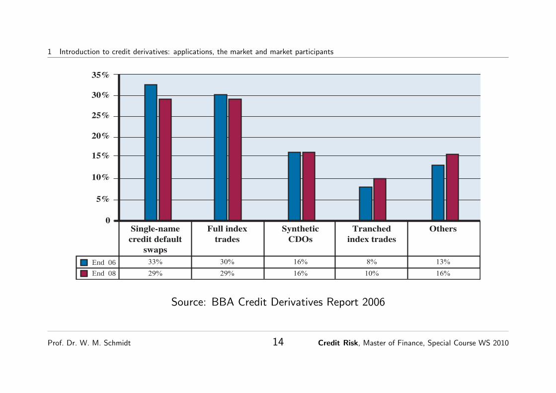
4. Product rangeIn line with the view of the BBA Credit Derivatives Panel, the range of products included in the surveyquestionnaire has been heavily revised to reflect current market trends. Single name credit default swapsstill represent a substantial section of the market, however the share has fallen to 33%. Index trades havebecome the second largest product representing 30% as at Q1 2006. The last two years have seen atremendous increase in the speed of development of credit derivatives products, with continuing diversi-fication expected. Synthetic CDOs (collateralised debt obligation) have continued to maintain position at16% of the market.
Credit Derivatives Products
British Bankers’ Association – Credit Derivatives Report 2006
6
0
5%
10%
15%
20%
25%
30%
35%
End 06
End 08
Single-name
credit default
swaps
33%
29%
Full index
trades
30%
29%
Synthetic
CDOs
16%
16%
Tranched
index trades
8%
10%
Others
13%
16%
Type 2000 2002 2004 2006
Basket products 6.0% 6.0% 4.0% 1.8%
Credit linked notes 10.0% 8.0% 6.0% 3.1%
Credit spread options 5.0% 5.0% 2.0% 1.3%
Equity linked credit products n/a n/a 1.0% 0.4%
Full index trades n/a n/a 9.0% 30.1%
Single-name credit default swaps 38.0% 45.0% 51.0% 32.9%
Swaptions n/a n/a 1.0% 0.8%
Synthetic CDOs – full capital n/a n/a 6.0% 3.7%
Synthetic CDOs – partial capital n/a n/a 10.0% 12.6%
Tranched index trades n/a n/a 2.0% 7.6%
Others 41.0% 36.0% 8.0% 5.7%
Source: BBA Credit Derivatives Report 2006
Prof. Dr. W. M. Schmidt 13 Credit Risk, Master of Finance, Special Course WS 2010
1 Introduction to credit derivatives: applications, the market and market participants
activity due to ‘Banks – Trading Activities’ and ‘Banks – Loan Portfolio’ to provide an emphasis on whyactivity was taking place rather than a distinction between the types of banks involved. This has high-lighted that almost two thirds of banks’ derivatives volume is due to trading and a third is related to theirloan book.
4. Product rangeIn line with the view of the BBA Credit Derivatives Panel, the range of products included in the surveyquestionnaire has been heavily revised to reflect current market trends. Single name credit default swapsstill represent a substantial section of the market, however the share has fallen to 33%. Index trades havebecome the second largest product representing 30% as at Q1 2006. The last two years have seen atremendous increase in the speed of development of credit derivatives products, with continuing diversi-fication expected. Synthetic CDOs (collateralised debt obligation) have continued to maintain position at16% of the market.
Credit Derivatives Products
British Bankers’ Association – Credit Derivatives Report 2006
6
0
5%
10%
15%
20%
25%
30%
35%
End 06
End 08
Single-name
credit default
swaps
33%
29%
Full index
trades
30%
29%
Synthetic
CDOs
16%
16%
Tranched
index trades
8%
10%
Others
13%
16%
Type 2000 2002 2004 2006
Basket products 6.0% 6.0% 4.0% 1.8%
Credit linked notes 10.0% 8.0% 6.0% 3.1%
Credit spread options 5.0% 5.0% 2.0% 1.3%
Equity linked credit products n/a n/a 1.0% 0.4%
Full index trades n/a n/a 9.0% 30.1%
Single-name credit default swaps 38.0% 45.0% 51.0% 32.9%
Swaptions n/a n/a 1.0% 0.8%
Synthetic CDOs – full capital n/a n/a 6.0% 3.7%
Synthetic CDOs – partial capital n/a n/a 10.0% 12.6%
Tranched index trades n/a n/a 2.0% 7.6%
Others 41.0% 36.0% 8.0% 5.7%
Source: BBA Credit Derivatives Report 2006
Prof. Dr. W. M. Schmidt 14 Credit Risk, Master of Finance, Special Course WS 2010
1 Introduction to credit derivatives: applications, the market and market participants
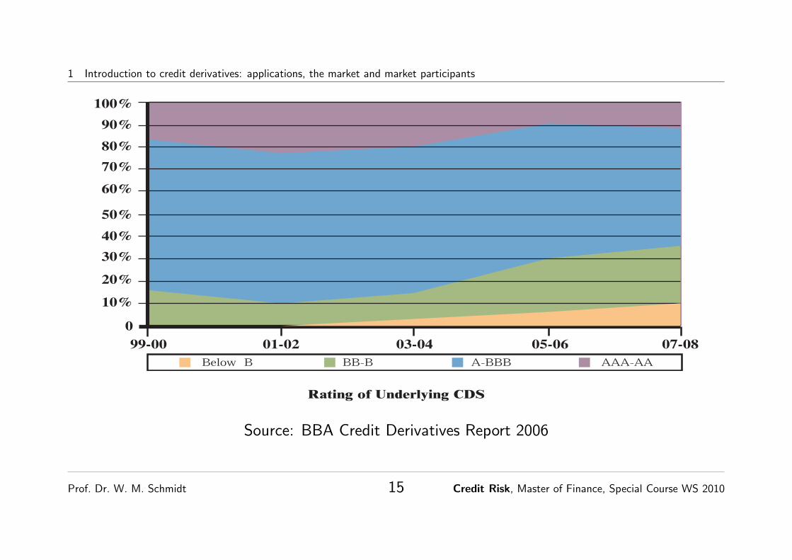
5. Rating of underlying assets
In this year’s survey a much more granular view has been taken of the ratings of the underlying assets thanpreviously. Underlying ratings of assets in CDS and Indices are now split out. Overall there has been adownward migration of average rating of underlying assets. For CDS the AAA – BBB category has fallenfrom 65% in 2004 to 59% in 2006 and this is estimated to continue to fall to 52% by end of 2008.Conversely the BB - B category has expanded from 13% to 23% and is expected to continue to grow to27% by end 2008.
Rating of Underlying CDS
6. Credit events
Every respondent has experienced credit events that triggered payment over the period. The highestnumber of credit events occurred in the high yield sector. There was an even spread of events across thecategories specified: Investment grade Europe, Investment grade US, Emerging markets, high yield,Asia/Australia and other. Delphi, Dana Corp, and Delta were the credits most frequently referred to as trig-gering payment.
7. Payouts
In contrast to the 2004 survey physical settlement has dropped from 86% down to 73%. The main shifthas been toward cash settlement which has more than doubled to 23% from 11% last year. Fixed amountsettlement remained the same at 3%. Quarterly settlement has continued to have an impact on firms.
Selected Participant Comment:
1. In the long term, the move to quarterly settlement will improve credit derivatives markets by increasingstandardization of product, which in turn drives liquidity. In the short term, quarterly settlement has madethe business more operationally intensive which has increased costs. Therefore, the short term benefit isless clear given the increased operational intensity.
British Bankers’ Association – Credit Derivatives Report 2006
7
0
10%
20%
30%
40%
50%
60%
70%
80%
90%
100%
99-00 01-02 03-04 05-06 07-08
Below B BB-B A-BBB AAA-AA
Source: BBA Credit Derivatives Report 2006
Prof. Dr. W. M. Schmidt 15 Credit Risk, Master of Finance, Special Course WS 2010
2 The first credit derivative: asset swap
Time to maturity of CDS are mainly 5 years and with increasing liquidity in 3 and 7-10 years.
Major market participants are banks, insurance companies, corporates, hedge funds and
pension funds. Banks are protection buyers as well as protection sellers whereas insurance
companies are mainly protection sellers. Hedge funds enter into CDS as protection seller for yield
enhancement or leverage, or as protection buyer, e.g., in case of convertible bonds arbitrage.
2 The first credit derivative: asset swap
The purpose of an asset swap is to exchange the fixed coupons of a bond versus Libor ± some
corresponding spread. The intention of the investor owning the fixed coupon bond is basically
to exchange that bond for a par floater with the same default risk and same maturity. Since
the exchange of the notional amount of both bonds cancel out, what is left is just the exchange
of the fixed versus floating coupons. Motivation of the transaction is to reduce the sensitivity
of the investment with respect to changes in market interest rates, since the floater has almost
Prof. Dr. W. M. Schmidt 16 Credit Risk, Master of Finance, Special Course WS 2010

2 The first credit derivative: asset swap
(depending on the spread) no duration. On the other hand, the spread over Libor extracts the
premium paid in return for taking the default risk.
Contrary to a plain interest rate swap there are some tricky details to take care of which
are necessary to achieve the above goal of the transaction. We discuss the most popular type
of an asset swap, the so-called par-par asset swap. First, at inception of the asset swap there
is an upfront payment of dirty price Pd of the bond minus 100 (par). In principle this can be
interpreted as the investor selling his bond at Pd and buying at the same time a par floater. On
the fixed side of the swap there is always a full first coupon payment, even if the swap start is
somewhere in the middle of a coupon period. However, on the floating side there is normally a
short first floating period ranging from the asset swap start to the first regular fixed coupon date:
Prof. Dr. W. M. Schmidt 17 Credit Risk, Master of Finance, Special Course WS 2010

2 The first credit derivative: asset swap
-time
swap start
6
dirty price - 100
6
6 6 6
? ?
maturityof the bond
6
?
+100
-100coupon payments
Libor ± spread s
Evaluating an asset swap just requires discounting its cash flows with the discount factors of the
Prof. Dr. W. M. Schmidt 18 Credit Risk, Master of Finance, Special Course WS 2010
2 The first credit derivative: asset swap
interest rate swap curve(!)
Pd − 100 + (present value of Libor +s payments)− (present value of fixed coupon payments)
= Pd − 100 + PVswap curve(Libor) + PVswap curve(spread s)− PVswap curve(fixed coupons)
= Pd − 100 + PVswap curve(Libor) + PVswap curve(100) + PVswap curve(spread s)
−PVswap curve(fixed coupons)− PVswap curve(100)
= Pd − PVswap curve(fixed bond) + PVswap curve(spread s).
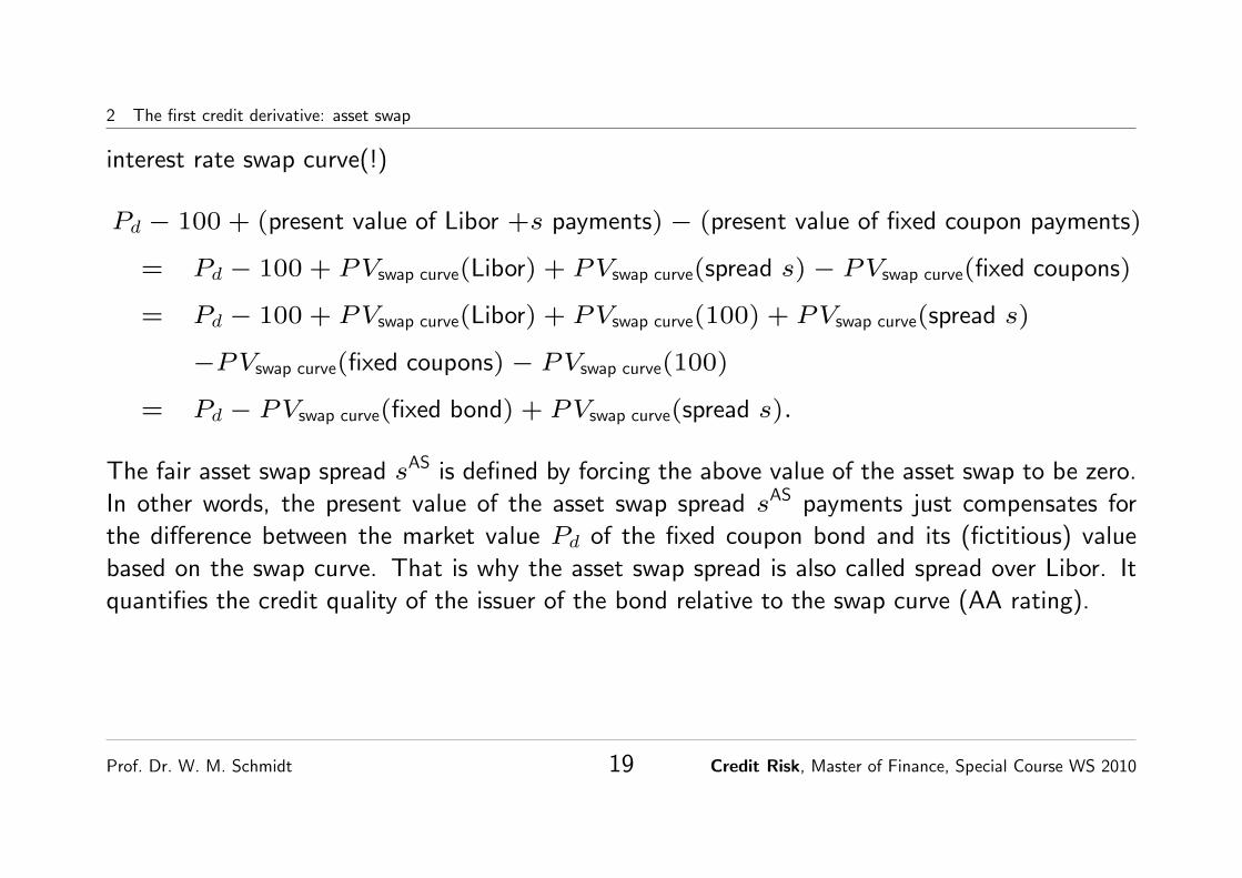
The fair asset swap spread sAS is defined by forcing the above value of the asset swap to be zero.
In other words, the present value of the asset swap spread sAS payments just compensates for
the difference between the market value Pd of the fixed coupon bond and its (fictitious) value
based on the swap curve. That is why the asset swap spread is also called spread over Libor. It
quantifies the credit quality of the issuer of the bond relative to the swap curve (AA rating).
Prof. Dr. W. M. Schmidt 19 Credit Risk, Master of Finance, Special Course WS 2010

2 The first credit derivative: asset swap
Often, asset swaps are traded as so-called packages, i.e., the underlying fixed coupon bond
plus the asset swap. At inception an asset swap package is always worth par. The investor gets a
synthetic default risky par floater paying Libor plus asset swap spread.
Computer Exercise 2.1. Calculate the fair asset swap spread for a bond with annual coupon
of C = 5%, issue date of the bond 20.04.1999 and time to maturity 10 years. Today the bond
trades at a (clean) price of 103,31. Use the EXCEL sheet ZinsPricer.xls with the given swap
curve there.
Prof. Dr. W. M. Schmidt 20 Credit Risk, Master of Finance, Special Course WS 2010

3 Credit default swaps
3 Credit default swaps
3.1 First applications, cash flows and quotation
In a credit default swap (CDS) counter party A pays an insurance premium to counter party Band receives in return some payment from B in case a specified credit event (related to some
entity C) takes place during the lifetime of the swap. Normally the credit event is the default of
one or more underlying reference assets (e.g., bonds) issued by a certain reference entity C.
A credit default swap is nothing else but an insurance contract. The protection buyer Apays an insurance fee (premium, spread) and receives in return from the protection seller Bcompensation for the loss in case the insured event happens.
The (insurance) premium is quoted in basis points referring to some notional amount and is
paid on a regular basis during the life time of the CDS.
If the insured event takes place during the life time of the CDS the protection buyer normally
Prof. Dr. W. M. Schmidt 21 Credit Risk, Master of Finance, Special Course WS 2010

3 Credit default swaps 3.1 First applications, cash flows and quotation
delivers the defaulted reference asset (or some other qualified equivalent asset) with the agreed
notional amount and in return gets compensated by a payment of the full notional amount from
the protection seller. This is called physical settlement. Alternatively, one can agree on cashsettlement, that is, the cash amount of par minus the market price of the defaulted asset is paid
to the protection buyer. Most of the trades settle physically. However, if for example, the CDS is
part of a synthetic CDO construction then there will be cash settlement.
protection buyer protection seller
A-
�
premium (spread) s
in case of default: par - defaulted asset B
Prof. Dr. W. M. Schmidt 22 Credit Risk, Master of Finance, Special Course WS 2010

3 Credit default swaps 3.1 First applications, cash flows and quotation
To specify a credit default swap one has to determine the following terms of the trade:
• reference entity, reference assets, e.g., bonds issued by ABC,
• credit event to be insured, normally default,
• notional amount NPA, e.g., 10 Mio. EUR,
• start of the CDS, start of the spread payments, protection start T0,
• time to maturity Tn,
• frequency and day count convention of spread payments, e.g.,quarterly, act/360,
• premium, spread s, e.g., s = 1.00%,
• payment in case of insurance event and its settlement (physical, cash).
To simplify we will always think of the credit event as being just default of the reference
entity.
Prof. Dr. W. M. Schmidt 23 Credit Risk, Master of Finance, Special Course WS 2010

3 Credit default swaps 3.1 First applications, cash flows and quotation
The cash flows of a CDS can be visualized as follows. Starting with the start date T0 the spread
period dates T0, T1, . . . , Tn are determined according to the given frequency. Non-business days
are usually adjusted applying the convention Modified Following.
Denote by τ the time of default of the reference entity. Today the precise value of τ is
not known, it is a random variable. For entities with low default risk the probability that τ will
“happen” in the near future is very low.
-
T0 T1 T2 Tn
6 6 6
?
τ
66
. . .
Prof. Dr. W. M. Schmidt 24 Credit Risk, Master of Finance, Special Course WS 2010

3 Credit default swaps 3.1 First applications, cash flows and quotation
Payments to the protection seller
For each period [Ti−1, Ti] at the end Ti of the period the protection seller receives the
amount NPA s ∆i as long as there has been no default until Ti. Here ∆i denotes the length
of the period [Ti−1, Ti] according to the given day count convention. If there happens to be a
default inside the period [Ti−1, Ti], i.e., Ti−1 < τ < Ti, there will be normally a payment of the
spread accrued over the period [Ti−1, τ ]. The spread payments terminate at the time of default
or maturity whatever comes first.
Payments to the protection buyer
In case of a default during the lifetime of the CDS the protection buyer receives “at” the
time τ of default a compensation which is worth NPA(1 − R), where R denotes the recoveryrate. In case of cash settlement this is exactly the cash amount paid to the protection buyer,
for physical settlement the delivered defaulted reference asset is worth −NPAR for which the
protection buyer gets a compensation of NPA (par).
Prof. Dr. W. M. Schmidt 25 Credit Risk, Master of Finance, Special Course WS 2010

3 Credit default swaps 3.1 First applications, cash flows and quotation
The fair default swap spread sCDS (short: CDS spread) is defined by the fact that the
underlying CDS is worth zero, i.e., fair. In most cases, at inception of a CDS the premium is
agreed to be fair.
The market quotes credit default swaps by their fair spreads sCDS. We emphasize that fair
means that the market considers a CDS with this spread as being worth 0. We will have to
discuss later on what this means in relation to other products, e.g., asset swaps. Also observe the
analogy to interest rate swaps where the market quotes fair swap rates.
Prof. Dr. W. M. Schmidt 26 Credit Risk, Master of Finance, Special Course WS 2010

3 Credit default swaps 3.1 First applications, cash flows and quotation
Prof. Dr. W. M. Schmidt 27 Credit Risk, Master of Finance, Special Course WS 2010

3 Credit default swaps 3.1 First applications, cash flows and quotation
Remark:In addition to the credit risk of the reference entity of the CDS we are also facing a credit risk
with respect to the counter party. The default risk of the protection seller is obviously particularly
important. If the default of the reference entity is “highly correlated” with the default of the
protection seller, then the CDS gives basically no protection to the protection buyer. In the
following we will ignore the default risk of the CDS counter parties. In practice this risk is often
managed by requiring some collateral.
Exercise 3.1. Often default swaps are interpreted solely as insurance against default. Why is
this wrong and how does a CDS also offer insurance against changes in credit quality?
Prof. Dr. W. M. Schmidt 28 Credit Risk, Master of Finance, Special Course WS 2010

3 Credit default swaps 3.2 No-arbitrage relationships
3.2 No-arbitrage relationships
In this section we discuss the problem of what the fair premium (CDS spread) for protection in a
CDS should be.
The default risk of credit risky investments such as bonds is quantified by various different
notions of spread used by practitioners. There are, e.g., the so-called yield spread, asset swap
spread, discount spread etc. So how do these spreads relate to the CDS spread?
In our discussion we first assume an idealized market for getting some fundamental theoretical
insights into the relationship of the CDS spread to other spreads in the market. However, in
practice things get much more involved and in real life one often observes derivations from the
theoretical relationships. We shall investigate these problems afterwards.
The valuation of derivatives is based on the no-arbitrage principle. In the simplest case
an arbitrage is a clever combination of transactions which yields a risk free gain without any
investment. The market would exploit those opportunities immediately and in an idealized world
arbitrage opportunities do not exist, i.e., prices in the market are in an arbitrage free relationship.
Prof. Dr. W. M. Schmidt 29 Credit Risk, Master of Finance, Special Course WS 2010

3 Credit default swaps 3.2 No-arbitrage relationships
We start by discussing the so-called par-spread. Imagine there is a floating rate bond issued
by the reference entity of our credit default swap. The bond pays as coupon Libor + spread and
trades at a price of 100 (par). The corresponding spread is called the par-spread spar and the
bond is a par-floater.
We have the following relationship:
CDS Spread ≈ Par-Spread
Here is the argument: investing into a par floater and, at the same time, buying protection
on the issuer via a CDS yields an investment where the investor gets a net coupon payment of
Libor + (spar − sCDS
).
But the combined position consisting of the par floater and the CDS is equivalent to a risk free
floating rate bond. Indeed, in case of a default of the risky par floater the CDS will cover exactly
the loss and we will get always a full redemption of our investment. In a risk free floater the
Prof. Dr. W. M. Schmidt 30 Credit Risk, Master of Finance, Special Course WS 2010

3 Credit default swaps 3.2 No-arbitrage relationships
coupon is just Libor and therefore, to avoid arbitrage,
0 = spar − sCDS
.
Exercise 3.2. There are several gaps in the above argument, find out where! In particular
analyse exactly the cash flows of the involved transactions in the situation of a default.
Adapt the reasoning further, taking into account that buying the par floater the investor has to
finance the investment by his own refinancing conditions.
In reality par floaters rarely exist. The above discussion is just a preparation to analyse the
relationship between the CDS spread sCDS and the asset swap spread sAS.
As discussed in Section 2 an asset swap package can be seen as a synthetic par floater and
we get from that and the preceding discussion immediately the following relationship:
Prof. Dr. W. M. Schmidt 31 Credit Risk, Master of Finance, Special Course WS 2010

3 Credit default swaps 3.2 No-arbitrage relationships
CDS Spread ≈ Asset Swap Spread
But again there are several gaps in the argument. Compared to a par floater the behavior of
the asset swap package in default is different. If there happens to be a default of the underlying
bond the investor of the asset swap package receives the recovery from the bond, but in addition
to that he is still exposed as a fixed rate (coupon) payer in the interest rate swap. Depending
on the prevailing market conditions (swap curve) the interest rate swap has some (positive or
negative) market value contributing to the overall recovery of the package.
Anyway, independently of the many details to take into account, the asset swap spread gives
a first rough indication what the fair CDS spread should be.
Prof. Dr. W. M. Schmidt 32 Credit Risk, Master of Finance, Special Course WS 2010

3 Credit default swaps 3.3 The cash–CDS basis, CDS strategies of market participants
3.3 The cash–CDS basis, CDS strategies of market participants
In practice one observes quite often significant differences between the quoted fair CDS premiums
and the spreads in the cash market (bonds, asset swaps). This difference is called the cash–CDSbasis. The reasons for these differences are mainly supply and demand (liquidity) in the different
markets. Theoretically this would yield arbitrage opportunities but in reality one is in most cases
not able to take advantage of them.
The following table shows observed differences between the CDS spread and the asset swap
spread as quoted in the market.
Prof. Dr. W. M. Schmidt 33 Credit Risk, Master of Finance, Special Course WS 2010

3 Credit default swaps 3.3 The cash–CDS basis, CDS strategies of market participants
Default Swap Asset Swap Basis
Bid/Offer Bid/Offer (Bid-Offer)
Bank of America 48/55 46/43 5
Bank One Corp 60/75 65/60 0
Chase Corp 40/48 35/30 10
Citigroup 38/45 30/27 11
First Union 68/85 66/63 5
Goldman 45/55 46/41 4
Lehman Br 70/80 68/63 7
Merrill Lynch 40/50 28/23 17
Morgan Stanley 45/55 28/23 22
The basis, i.e., CDS minus asset swap spread, can be both, positive or negative. For the
telecommunication sector the basis was as high as 80 basis points as observed in February 2001
for Deutsche Telekom. However, as a result of relative value strategies exploited by market
participants the basis stays inside certain bounds.
Prof. Dr. W. M. Schmidt 34 Credit Risk, Master of Finance, Special Course WS 2010

3 Credit default swaps 3.3 The cash–CDS basis, CDS strategies of market participants
For example, in case the basis is positive, i.e., sCDS > sAS, one could try to realize an
arbitrage gain by selling protection and at the same time shorting the bond. However, in practice
shorting a bond is not easy and may require additional costs so this theoretical arbitrage strategy
can often not be realized. In general a CDS is the perfect instrument to short credit risk by buying
protection whereas in the cash market it is difficult to enter into a negative credit exposure.
There are typical situations where the demand for buying protection is particularly high and
therefore the CDS spreads are rising. One example is when convertible bonds are newly issued:
Prof. Dr. W. M. Schmidt 35 Credit Risk, Master of Finance, Special Course WS 2010

3 Credit default swaps 3.3 The cash–CDS basis, CDS strategies of market participants
Credit Default Swap Handbook – 31 January 2002
19
opportunities to sell protection and generate compelling relative value.
A typical situation where such a discrepancy can occur is during and following theissuance of a convertible bond. In such circumstances CB investors may look tounlock “cheap” equity volatility by hedging credit risk – the credit derivativemarket typically offers the most effective means of doing this quickly in largesize. Another factor that can drive default swap spreads on a broader range ofcredits is the launch of large synthetic CDO transactions. In order to sell syntheticcredit risk into these structures, the originating investment banks will typicallyhave to build up long credit positions (sell protection) before or immediately afterthe transaction which will tend to pull default swap spreads tighter. Sometimesthe investment bank may buy this credit exposure in the cash market but theliquidity for major names in the default swap market combined with a wish toavoid basis risk tends to favour selling protection.
Chart 18: Fiat Default Swap Basis Widened Sharply Following Its CB Issue
50
70
90
110
130
150
170
190
210
16-Oct-01 30-Oct-01 13-Nov-01 27-Nov-01 11-Dec-01 25-Dec-01 8-Jan-02 22-Jan-02
5yr Default FIAT 5.75% May-2006 Asset Swap
Spread (bp)
Source: Merrill Lynch
� Unfunded vs. Funded
A key difference between selling protection and buying an asset swap is that thedefault swap is unfunded. However, due to the nature of the transaction, theprotection seller is effectively locking a spread above LIBOR. Thus for aninvestor which is funded above LIBOR selling protection tends to be particularlyattractive. In our opinion, this represents a key advantage for the synthetic marketfor two reasons:
1. Most market participants and “street” trading desks fund their credit books atspreads above LIBOR. Default swaps therefore give the opportunity ofgenerating greater carry than similarly yielding asset swaps.
2. Losing the necessity to fund the credit purchase, makes it easier for creditbuyers to leverage their credit views without actually borrowing.
� Investment Flexibility
We believe that a major advantage of default swaps for credit investors is that theycan greatly enhance investment flexibility for investors who are reliant wholly onthe cash market.
Default swaps offer a means of taking a generic credit view on a Reference Entity.This is probably most important when that view is negative, as buying protectionis typically much more straightforward than borrowing and shorting bonds. Inaddition to outright bear strategies, this can be extremely useful for holders ofilliquid securities (such as loans) who wish to hedge credit exposure. Indeed the
…notably from new-issue CBsand synthetic CDOs
Default swaps effectively lockin funding at libor
Easier to short credit…
Fiat issues a $2.2bnConvertible Bond
In the process of arranging a synthetic CDO the bank issuing the CDO has to synthesize
the credit risk of the pool by selling protection in the CDS market. This causes CDS spreads to
decline.
Prof. Dr. W. M. Schmidt 36 Credit Risk, Master of Finance, Special Course WS 2010

3 Credit default swaps 3.3 The cash–CDS basis, CDS strategies of market participants
The strategies of the market participants are heavily dependent to their funding costs. For
a bank with funding above Libor entering into a CDS selling protection normally yields higher
returns as compared to entering into a cash position (bond).
Whenever the CDS spread trades below the asset swap spread there is the following arbitrage
strategy. Suppose the investors funding is L+ x (L=Libor) and the bond pays in the asset swap
L+ sAS. Now in case that
sCDS
< sAS − x
the investor can realize a risk free gain of sAS − x − sCDS > 0 by entering into the asset swap
and buying protection in the CDS market. Therefore the basis between CDS and asset swap is
bounded below by the funding spread of the “best” market player.
Exercise 3.3. Think again if the gain of the above strategy really risk-free?
Prof. Dr. W. M. Schmidt 37 Credit Risk, Master of Finance, Special Course WS 2010

3 Credit default swaps 3.4 Credit linked notes, funded CDS
3.4 Credit linked notes, funded CDS
Credit defaults swap are not only used to buy or sell insurance on existing default risky positions,but also to create interesting new investment opportunities. This is done by so-called CreditLinked Notes (CLN).
default swap B CLN investor
bond A
-
�
-
�
6
?
payment in default
spread s
100
C + s
100 C
Prof. Dr. W. M. Schmidt 38 Credit Risk, Master of Finance, Special Course WS 2010

3 Credit default swaps 3.4 Credit linked notes, funded CDS
A credit linked note can be seen as a synthetic bond whose credit risk is linked to some
reference entity. Investing in a credit linked note the investor gets a package consisting of a
(usually “risk free”) bond issued by some issuer A, e.g., a bond issued by a AA bank or a
Pfandbrief etc., but in addition to that the investor enters into a credit default swap selling
protection on the default of some reference B. From the CDS the investor receives the premium
payments s which, together with the coupon C of the bond, yield an overall coupon of C + s.
In case of a default of the reference B of the CDS the risk free bond is sold to cover the losses
from the CDS and the remaining proceeds are the recovery of the credit linked note. In principle
the investor of a CLN is exposed to the default risk of both, the issuer of the bond A and the
reference B of the CDS.
Credit linked notes are a powerful tool to create synthetic default risky bonds with any
maturity and currency, which are otherwise not available in the market.
Entering into a CLN requires an initial investment by the investor. That is why a CLN is also
called a funded CDS. The underling risk free bond serves as a kind collateral for the credit risk
the protection buyer in the CDS runs with respect to the investor.
Prof. Dr. W. M. Schmidt 39 Credit Risk, Master of Finance, Special Course WS 2010

4 Mark-to-market and the CDS curve
4 Mark-to-market and the CDS curve
In the previous section we investigated the relationship between the CDS and the asset swap
spread. These relative value relationships together with supply and demand in the market yield
the market quoted fair CDS spreads.
If we are looking for a CDS today the market gives us directly the corresponding fair premium
for buying or selling protection.
Observe again the analogy to the interest rate swap market where the market quotes directly
the fair swap rates which are a result of supply and demand in the swap market and of relative
value relationships to the bond market.
The problem of evaluating a credit default swap appears only if we are looking for a re-
evaluation of an existing CDS position relative to the actual market (mark-to-market). The
primary input into the valuation are the currently quoted fair CDS premiums. Depending on the
Prof. Dr. W. M. Schmidt 40 Credit Risk, Master of Finance, Special Course WS 2010

4 Mark-to-market and the CDS curve 4.1 Pricing directly from spread differences
difference between the spread in our existing CDS position and the quoted fair market spread, the
position possesses a positive or negative market value.
4.1 Pricing directly from spread differences
Imagine some time ago we have entered into a CDS with initial maturity Tn where we pay a
spread s0 (at inception of the trade this was the fair premium) for protection. Today, at time
t, the life time of the CDS has shortened to Tn − t. Suppose the market quotes today for a
Tn − t maturity CDS a fair premium of st. Then the difference st − s0 “counted” over the
remaining life time Tn − t should give us about the market value of our CDS position. In case
the actual spread st is higher than the spread s0 in the CDS the market value of the position
should be positive. Indeed, today in the market one would have to pay a much higher premium
st for protection compared to what we have to pay in our existing CDS. Our gain relative to the
market is the difference (st − s0) over the remaining life time. In case the actual market spread
st is below our premium s0, the CDS has a negative mark-to-market value.
Prof. Dr. W. M. Schmidt 41 Credit Risk, Master of Finance, Special Course WS 2010
4 Mark-to-market and the CDS curve 4.1 Pricing directly from spread differences
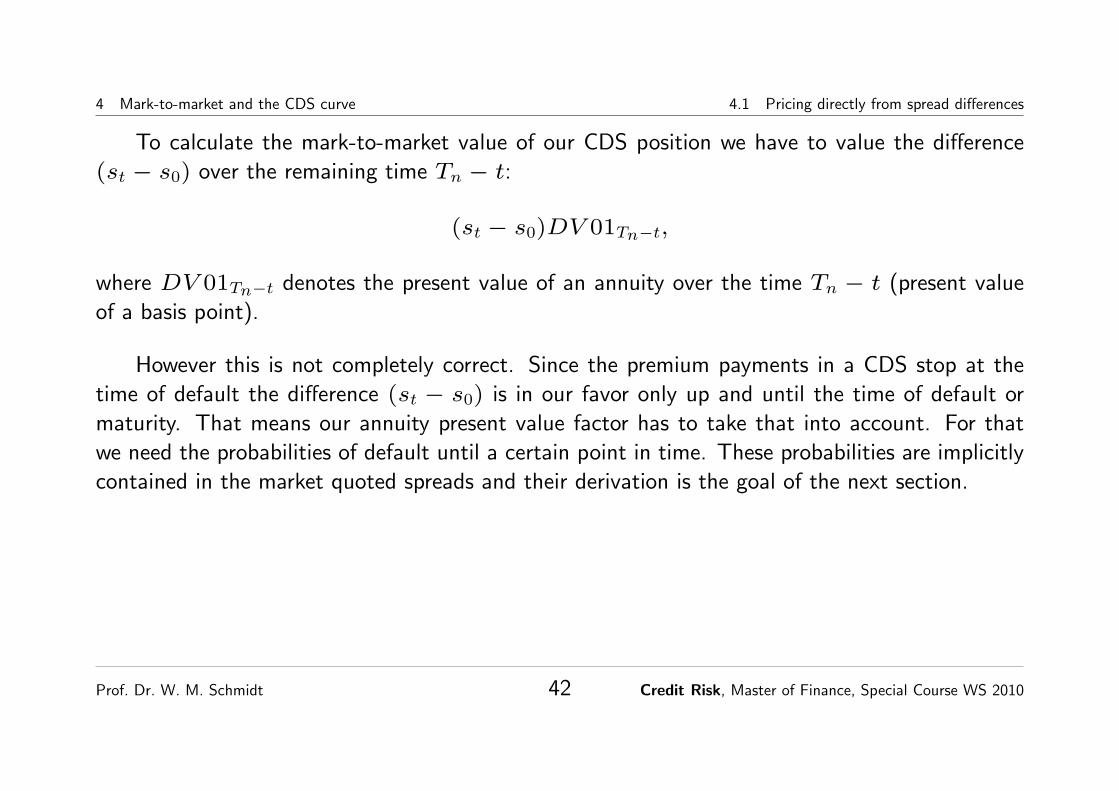
To calculate the mark-to-market value of our CDS position we have to value the difference
(st − s0) over the remaining time Tn − t:
(st − s0)DV 01Tn−t,
where DV 01Tn−t denotes the present value of an annuity over the time Tn − t (present value
of a basis point).
However this is not completely correct. Since the premium payments in a CDS stop at the
time of default the difference (st − s0) is in our favor only up and until the time of default or
maturity. That means our annuity present value factor has to take that into account. For that
we need the probabilities of default until a certain point in time. These probabilities are implicitly
contained in the market quoted spreads and their derivation is the goal of the next section.
Prof. Dr. W. M. Schmidt 42 Credit Risk, Master of Finance, Special Course WS 2010

4 Mark-to-market and the CDS curve 4.2 Deriving the default probabilities from market data
4.2 Deriving the default probabilities from market data
We use the following notation
DF(t) discount factor for time t as derived form the interest rate swap curve,
τ random time of default ,
q(t) = P(τ > t) survival probability for time t,
R recovery rate.
The present value of a default risky cash flow of one unit at time T is then
DF(T )q(T ),
i.e., the cash flow has to be discounted by the risk free discount factor and in addition it has to
be multiplied with the probability that the default does not happen until time T . Observe here
the qualitative analogy between a discount factor and a survival probability. Multiplying with the
survival probability is a kind of “additional discounting” for the default risk of the cash flow1.1Mathematically the multiplication of the discount factor and the survival probability assumes independence between riskless interest
Prof. Dr. W. M. Schmidt 43 Credit Risk, Master of Finance, Special Course WS 2010

4 Mark-to-market and the CDS curve 4.2 Deriving the default probabilities from market data
The (cumulative) probability of default until time T can be easily calculated from the survival
probability as
1− q(T ).
The risk free present value factor for an annuity with period length ∆i is defined as
DV 01Tn−t =∑Ti>t
∆iDF(Ti).
For a corresponding annuity which stops at the time of default we have
DV 01riskyTn−t =
∑Ti>t
∆iDF(Ti)q(Ti).
To calculate the mark-to-market value of our existing CDS position we have to utilize the risky
present value of a basis point
(st − s0)∑Ti>t
∆iDF(Ti)q(Ti).
rates and defaults.
Prof. Dr. W. M. Schmidt 44 Credit Risk, Master of Finance, Special Course WS 2010

4 Mark-to-market and the CDS curve 4.2 Deriving the default probabilities from market data
The question is now: where do we get the appropriate default or, equivalently, survival
probabilities from?
These probabilities are implicitly contained in the market prices such as prices of default risky
bonds or fair CDS premiums.
However, market prices or spreads reflect simultaneously the probability of default as well as
the potential recovery value in case of default. To extract the default probabilities we are forced
to make an assumption on the recovery rate R, for example, we could assume R = 15%. We
will have to discuss the implications of those assumptions later.
Prof. Dr. W. M. Schmidt 45 Credit Risk, Master of Finance, Special Course WS 2010

4 Mark-to-market and the CDS curve 4.2 Deriving the default probabilities from market data
To start with, consider the market price of a default risk bond. How do the survival
probabilities and the recovery rate R enter into the price of a bond with coupon C and face
value of 1? The dirty price Pd of the bond is given by the equation
Pd = C∑i
∆iDF(Ti)q(Ti) + DF(Tn)q(Tn) + R
∫ Tn
T0
DF(u)[q(u)− q(u+ du)]. (1)
The coupon payments and the redemption of the face value have to be discounted by the riskless
discount factors and the survival probabilities. The last expression in the equation above needs
some more explanation. It is the present value of the recovery ”payment”. At the time of default
the investor get paid the recovery rate R. Since we do not know if and when there will be a
default we have to consider all points in time u from T0 to Tn. If the default occurs at time u
we have to discount the recovery with the discount factor DF(u). The probability of a default
around time u, more precisely in the small interval [u, u + du], is just (q(u) − q(u + du)).
All those contributions have to be added up over all points u in time between T0 and Tn.
Prof. Dr. W. M. Schmidt 46 Credit Risk, Master of Finance, Special Course WS 2010

4 Mark-to-market and the CDS curve 4.2 Deriving the default probabilities from market data
Given the market price Pd of the bond, the curve of riskless discount factors DF(t) and
making an assumption on the recovery rate R, the market implied default probabilities have to
satisfy the pricing equation (1). Now we can try to “solve” this equation for the unknown default
probabilities.
Exercise 4.1. Given the market price of a default risky bond. To extract the implied default
probabilities we have to make a guess on the unknown recovery rate R, lets say R = 15%. How
will the implied default probabilities change if we make a different assumption on the recovery, for
example R = 30%. Will the corresponding default probabilities be higher or lower?
Since our main goal is the valuation of credit default swaps and since the CDS market quotes
the fair premiums we will be more interested in getting the default probabilities extracted from
the CDS market and not from prices of bonds (recall that there is often a significant difference
between the cash and the CDS market!).
Prof. Dr. W. M. Schmidt 47 Credit Risk, Master of Finance, Special Course WS 2010

4 Mark-to-market and the CDS curve 4.2 Deriving the default probabilities from market data
The CDS market quotes fair premiums (spreads). If we denote by s(n) the fair premium for
maturity Tn, the following equality has to be fulfilled
0 = − value of premium flows s(n)
+ value of the payment (1− R) at default
= −s(n)
n∑i=1
∆iDF(Ti)q(Ti)− s(n)
n∑i=1
∫ Ti
Ti−1
∆i
u− Ti−1
Ti − Ti−1
DF(u)[q(u)− q(u+ du)]
+(1− R)
∫ Tn
T0
DF(u)[q(u)− q(u+ du)]
≈ −s(n)
n∑i=1
∆iDF(Ti)q(Ti)− s(n)
n∑i=1
∆i
2DF
(Ti−1 + Ti
2
)[q(Ti−1)− q(Ti)]
+(1− R)
n∑i=1
DF
(Ti−1 + Ti
2
)[q(Ti−1)− q(Ti)]. (2)
Prof. Dr. W. M. Schmidt 48 Credit Risk, Master of Finance, Special Course WS 2010

4 Mark-to-market and the CDS curve 4.2 Deriving the default probabilities from market data
Again we have obtained an equation which we can try to resolve for the implied default
probabilities.
If there is a quoted fair spread s(1), . . . , s(n) for every maturity T1, . . . , Tn the
corresponding probabilities q(T1), . . . , q(Tn) can be extracted by a bootstrapping algorithm.
This is quite similar to the calculation of the riskless discount factors from the interest rate swap
curve.
Lets illustrate this by an example. For the first grid point T1 equation (2) reduces to
0 = −s(1)∆1DF(T1)q(T1)−s(1)∆1
2DF(T1/2)(1−q(T1))+(1−R)DF(T1/2)(1−q(T1)).
Observe that (1− q(T1)) is just the probability of a default during the interval (0, T1).
Computer Exercise 4.2. Consider a credit default swap with 1Y time to maturity, T1 = 1,
which starts today at T0 = 0. Let the fair premium quoted in the market be s(1) = 1%. We
assume for simplicity that the premium is paid annually with a 30/360 day count convention,
i.e., ∆1 = 1. From the interest rate swap curve the following discount factors are given
Prof. Dr. W. M. Schmidt 49 Credit Risk, Master of Finance, Special Course WS 2010

4 Mark-to-market and the CDS curve 4.2 Deriving the default probabilities from market data
DF(0.5) = 0, 9853,DF(1) = 0, 9714. For the recovery rate we assume R = 15%.
Calculate the implied survival probability q(1) for 1 year! How does the result change if we
assume a recovery of R = 30%?
Once the survival probabilities q(T1), . . . , q(Tn) for the grid points T1, . . . , Tn have been
extracted from the market spreads, we have to define a method to interpolate the survival
probability. For a time point t ∈ (Ti−1, Ti) the survival probability q(t) is interpolated according
to the formula
q(t) = q(Ti−1) exp(−λi(t− Ti−1)), t ∈ (Ti−1, Ti),
with
λi = ln
(q(Ti−1)
q(Ti)
)/(Ti − Ti−1).
The quantity λi is also called the default rate or default intensity (hazard rate) for the interval
[Ti−1, Ti]. The probability of a default during a small interval [t, t + ∆] given that there has
been no default so far is approximately λ∆; we will discuss this in more detail in Section 7.1.
Summarizing, survival probabilities are interpolated assuming a constant default rate in the
intervals [Ti−1, Ti].
Prof. Dr. W. M. Schmidt 50 Credit Risk, Master of Finance, Special Course WS 2010
4 Mark-to-market and the CDS curve 4.2 Deriving the default probabilities from market data
Remarks1. How should one interpret the default or survival probabilities which have been extracted from
the market? These probabilities are market implied probabilities, i.e., they reflect the opinion
of the market on the risk of default. They are not necessarily related to the “true” default
probabilities which are anyway not accessible at all! Out of historical data one can estimate
empirical default probabilities which might be a reasonable indication for the “true” probabilities.
However, the valuation of credit derivatives is based on the general principles of dynamic hedging
and arbitrage free pricing. Therefore for the purpose of valuation one has to utilize probabilities
as extracted from prices of traded instruments.
2. In the framework of risk-neutral valuation the price of a derivative is its “discounted”
expectation under the risk neutral distribution. In that context the market implied probabilities
can be seen as risk-neutral default probabilities.
3. The extracted survival probabilities where always “relative” to the interest rate swap curve
which has been interpreted as risk free. Recall that the price of a default risk payment of one
unit at time T was written as DF(T )q(T ). The default risk of the interest rate swap curve (AA
curve) relative to a truly default free discount curve (e.g. from government bonds) is already
“contained” in the discount factor DF(T ).
Prof. Dr. W. M. Schmidt 51 Credit Risk, Master of Finance, Special Course WS 2010

4 Mark-to-market and the CDS curve 4.3 Mark-to-market valuation of credit default swaps
4.3 Mark-to-market valuation of credit default swaps
In the previous section we have learned how to build the curve of market implied survival
probabilities. Now the valuation of any credit default swap is straightforward. We utilize the
curve of survival probabilities q(t), the curve of risk free discount factors DF(t) from the interest
rate swap market and (of course!) the same assumption on the recovery rate R as used in the
process of extracting the probabilities from the market. The value of an arbitrary credit default
swap is then calculated from the formula2
−sn∑i=1
∆iDF(Ti)q(Ti)− sn∑i=1
∆i
2DF
(Ti−1 + Ti
2
)[q(Ti−1)− q(Ti)]
+(1− R)
n∑i=1
DF
(Ti−1 + Ti
2
)[q(Ti−1)− q(Ti)]. (3)
2As in (2) we have approximated the respective integrals bei their mid-point sums. So the result is in fact an (quite good) approximationof the true value.
Prof. Dr. W. M. Schmidt 52 Credit Risk, Master of Finance, Special Course WS 2010
4 Mark-to-market and the CDS curve 4.4 How critical are the assumptions on the recovery rate?
This formula assumes the position of a protection buyer. For the protection seller we have to
switch just signs.
Computer Exercise 4.3. Evaluate a 100 Mio 5Y CDS with a spread s = 80 basis points paid
semi annually act/360. Use the spread sheet CDSPricer.xls with the interest curve, default
curve and recovery rate as specified there.
4.4 How critical are the assumptions on the recovery rate?
Extracting the default probabilities from market data we had to make a subjective assumption on
the recovery rate R. Rating agencies have collected historical data on realized recoveries that
can be used as an indication on the level of recovery. In practice one assumes recoveries in the
range between 15% to 50%. In any case one should try to make a realistic assumption.
However, it not yet clear how sensitive our valuations are with respect to the assumed
recovery rate. Fortunately and at a first glance somewhat surprising it turns out that the results
Prof. Dr. W. M. Schmidt 53 Credit Risk, Master of Finance, Special Course WS 2010

4 Mark-to-market and the CDS curve 4.4 How critical are the assumptions on the recovery rate?
show very little sensitivity with respect to the assumed recovery. The reason is that the recovery
enters at two places where their impact is offsetting. First in the process of extracting the
probabilities from market data, and, secondly, in the mark-to-market valuation of a CDS. It is
clearly important to use one and the same recovery in both places. As long as the premium of
the underlying CDS is not extremely far away from the fair market premium the impact of the
recovery assumption is negligible.
Computer Exercise 4.4. Evaluate an existing CDS with remaining life time of 4Y. The spread
in the CDS is s = 2%. How does the mark-to-market value change of we change the assumed
recovery from R = 15% to R = 50% in both places, the default curve generation and the
mark-to-market valuation?
Remark. In contrast to standard credit default swaps there exist so-called Digital DefaultSwaps where the insurance payment in case of a default is not linked to the recovery of the
reference asset but is a predefined amount. The valuation of those products can be carried
out following exactly the same lines as for a standard CDS. However the valuation is now
quite sensitive to the recovery assumed for extracting the probabilities. In this case a realistic
assumption on the recovery is particularly important.
Prof. Dr. W. M. Schmidt 54 Credit Risk, Master of Finance, Special Course WS 2010

5 Lessons from the credit crisis
5 Lessons from the credit crisis
5.1 Issues highlighted by the crisis
Let us first summarize selected pros and cons on credit derivatives, in particular, CDS:
• Pro:
– Hedging of credit risk (buy protection); easy way to short credit exposure; means to
transfer the credit risk without transferring the underlying loan, bond etc.; enables financial
institutions to continue to make loans;
– Take on credit risk (sell protection), no funding needed; access to exposure even if no
client/business relationship;
– Efficient allocation of risk and capital; credit risks borne by those who are best able to bear
them;
– Smooth out fluctuations in regulatory capital accounts under mark-to-market accounting -
CDS hedges mtm of loans, bonds;
Prof. Dr. W. M. Schmidt 55 Credit Risk, Master of Finance, Special Course WS 2010

5 Lessons from the credit crisis 5.1 Issues highlighted by the crisis
– Liquid credit trading reveals valuable information about credit risk;
• Con:
– Size of CDS market created systemic risk for the economy;
– CDS create excessive risk;
– CDS are used to manipulate the market;
– Credit derivatives enabled the boom that finally led to the crisis;
– Warren Buffett (2002): CDS are “weapons of financial mass destruction”
– Buying protection without having exposure is like buying fire insurance on the house of the
neighbor→ sets wrong incentives;
We discuss the above criticisms and their role played in the crisis. See also [Stulz, 2009].
Size of CDS market threatens the economy:
Face value of outstanding CDS contracts exceed the volume of outstanding debt, but overall
CDS volume is deceptive - it consists of long and short credit risk positions! For example, A sells
protection on 100 Mio and hedges later by buying protection on 50 Mio yields a outstanding CDS
volume of 150 Mio but the net exposure is only 50 Mio.
Prof. Dr. W. M. Schmidt 56 Credit Risk, Master of Finance, Special Course WS 2010

5 Lessons from the credit crisis 5.1 Issues highlighted by the crisis
However, the true outstanding net exposure in the market was not transparent. Nowadays major
dealers register their trades with the Depository Trust & Clearing Corporation.
Risk Category / Instrument Jun 2007 Dec 2007 Jun 2008 Dec 2008 Jun 2009 Jun 2007 Dec 2007 Jun 2008 Dec 2008 Jun 2009
Total contracts 516,407 595,738 683,814 547,371 604,622 11,140 15,834 20,375 32,244 25,372
Foreign exchange contracts 48,645 56,238 62,983 44,200 48,775 1,345 1,807 2,262 3,591 2,470 Forwards and forex swaps 24,530 29,144 31,966 21,266 23,107 492 675 802 1,615 870 Currency swaps 12,312 14,347 16,307 13,322 15,072 619 817 1,071 1,421 1,211 Options 11,804 12,748 14,710 9,612 10,596 235 315 388 555 389
Interest rate contracts 347,312 393,138 458,304 385,896 437,198 6,063 7,177 9,263 18,011 15,478 Forward rate agreements 22,809 26,599 39,370 35,002 46,798 43 41 88 140 130 Interest rate swaps 272,216 309,588 356,772 309,760 341,886 5,321 6,183 8,056 16,436 13,934 Options 52,288 56,951 62,162 41,134 48,513 700 953 1,120 1,435 1,414
Equity-linked contracts 8,590 8,469 10,177 6,159 6,619 1,116 1,142 1,146 1,051 879 Forwards and swaps 2,470 2,233 2,657 1,553 1,709 240 239 283 323 225 Options 6,119 6,236 7,521 4,607 4,910 876 903 863 728 654
Commodity contracts 7,567 8,455 13,229 3,820 3,729 636 1,898 2,209 829 689 Gold 426 595 649 332 425 47 70 68 55 43 Other commodities 7,141 7,861 12,580 3,489 3,304 589 1,829 2,141 774 646
Forwards and swaps 3,447 5,085 7,561 1,995 1,772 Options 3,694 2,776 5,019 1,493 1,533
Credit default swaps 42,581 58,244 57,403 41,883 36,046 721 2,020 3,192 5,116 2,987 Single-name instruments 24,239 32,486 33,412 25,740 24,112 406 1,158 1,901 3,263 1,953 Multi-name instruments 18,341 25,757 23,991 16,143 11,934 315 862 1,291 1,854 1,034
Unallocated 61,713 71,194 81,719 65,413 72,255 1,259 1,790 2,303 3,645 2,868
Memorandum Item:
Gross Credit Exposure 2,672 3,256 3,859 4,555 3,744
Instrument / counterparty Jun 2007 Dec 2007 Jun 2008 Dec 2008 Jun 2009 Jun 2007 Dec 2007 Jun 2008 Dec 2008 Jun 2009
Total contracts 48,645 56,238 62,983 44,200 48,775 1,345 1,807 2,262 3,591 2,470
reporting dealers 19,173 21,334 24,845 18,810 18,891 455 594 782 1,459 892
other financial institutions 19,144 24,357 26,775 17,223 21,441 557 806 995 1,424 1,066
non-financial customers 10,329 10,548 11,362 8,166 8,442 333 407 484 708 512
Outright forwards and foreign
exchange swaps 24,530 29,144 31,966 21,266 23,107 492 675 802 1,615 870
reporting dealers 8,800 9,899 10,897 8,042 7,703 190 228 281 635 301
other financial institutions 10,010 13,102 14,444 8,646 10,653 185 292 348 636 374
non-financial customers 5,720 6,143 6,624 4,577 4,751 117 154 172 343 195
Currency swaps 12,312 14,347 16,307 13,322 15,072 619 817 1,071 1,421 1,211
reporting dealers 4,909 5,487 6,599 5,807 6,330 155 215 315 544 402
other financial institutions 5,262 6,625 7,367 5,610 6,717 291 406 520 627 568
non-financial customers 2,141 2,234 2,341 1,906 2,025 173 196 237 250 241
Options 11,804 12,748 14,710 9,612 10,596 235 315 388 555 389
reporting dealers 5,464 5,948 7,349 4,961 4,858 111 151 186 280 190
other financial institutions 3,872 4,629 4,964 2,968 4,071 81 108 127 161 125
non-financial customers 2,468 2,171 2,397 1,683 1,666 43 57 75 115 75
Notional amounts outstanding Gross market values
Table 20A: Amounts outstanding of OTC foreign exchange derivativesBy instrument and counterpartyIn billions of US dollars
Table 19: Amounts outstanding of over-the-counter (OTC) derivativesBy risk category and instrumentIn billions of US dollars
Notional amounts outstanding Gross market values
BIS Quarterly Review, December 2009 A 103
Source: BIS 2009
Prof. Dr. W. M. Schmidt 57 Credit Risk, Master of Finance, Special Course WS 2010
5 Lessons from the credit crisis 5.1 Issues highlighted by the crisis
CDS create excessive risk:
For each protection seller there is be a protection buyer. Defaults of the CDS reference entity
hurt the protection seller and benefit the buyer - on net it is a redistribution of wealth.
However, even if dealers hedge their positions by offsetting trades, there might be a
considerable counter party risk. Defaults of a dealer can cause unexpected havoc. Losses from
dealer default could be large, even with collateral agreements. Also large seller position carry
wrong way risk: a decline of the CDS reference entity might cause the credit worthiness of the
seller to decline as well.
Interconnections of large market players fed concerns that a default of a major player has
devastating effects in the whole sector, see the AIG case.
CDS are used to manipulate the market:
CDS are a measure of market sentiment of the credit worthiness and note a cause of corporate
ills.
[Mason, 2009]: “Blaming CDSs for corporate debt problems is like blaming the thermometer for
the temperature.”
Prof. Dr. W. M. Schmidt 58 Credit Risk, Master of Finance, Special Course WS 2010

5 Lessons from the credit crisis 5.2 Private sectors initiatives
Credit derivatives enabled the boom that finally led to the crisis:
Due to the separation of risk bearing from funding, lenders have less incentive to check the
quality of the borrower and to monitor the position. Example: hedging subprime mortgages with
CDS on subprime mortgage securitizations.
Huge investors demand for selling protection via the Subprime mortgage CDS ABX indices:
investors take more exposure than there were such mortgages.
Problems with the physical settlement of CDS:
If the volume of outstanding protection exceeds the volume of debt qualified for physical delivery
in case of default, physical settlement becomes problematic. This happened also for positions in
the subprime mortgage ABX indices.
5.2 Private sectors initiatives
In the meantime, most of the above issues have been addressed by the market.
In 2009 the International Swaps and Derivatives Association (ISDA), issued two amendments
Prof. Dr. W. M. Schmidt 59 Credit Risk, Master of Finance, Special Course WS 2010
5 Lessons from the credit crisis 5.2 Private sectors initiatives
to their CDS Master Agreement, the so called “big bang” and “small bang” protocols. The
agreements of these protocols came into force in June resp. July 2009.
The major changes are:
• Standardization of CDS contracts:
Fix spread payments of 25, 100, 500 or 100 bps (Europe), period dates 20th of
Mar/Jun/Sep/Dec., full first period
prices are settled by an upfront payment.
This allows for a perfect netting of cash flows for offsetting trades.
• Rolling lock back effective dates:
Protection effectively starts 60 days (credit events) and 90 days (succession events) before
trade date.
This leads to a better netting of yet unobserved credit events for offsetting trades.
• Quoting standards and standardized pricing:
In the past it was common to quote so-called par spreads. Since the spread payments are now
Prof. Dr. W. M. Schmidt 60 Credit Risk, Master of Finance, Special Course WS 2010
5 Lessons from the credit crisis 5.2 Private sectors initiatives
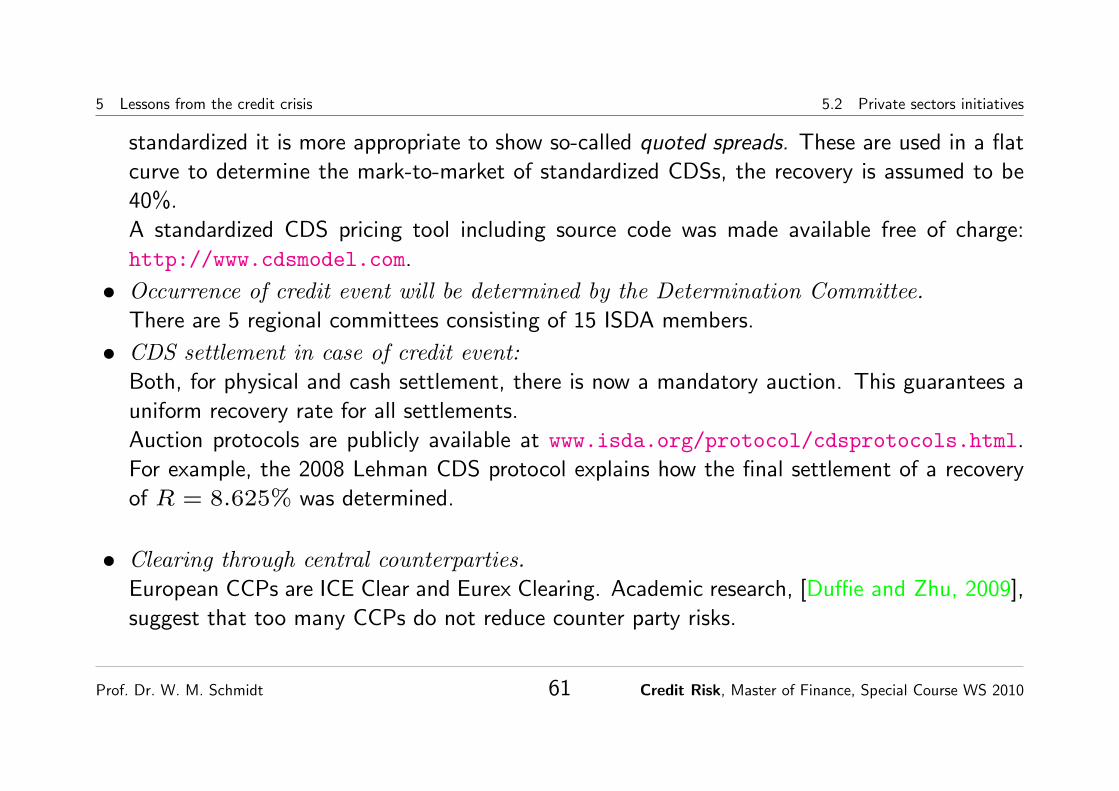
standardized it is more appropriate to show so-called quoted spreads. These are used in a flat
curve to determine the mark-to-market of standardized CDSs, the recovery is assumed to be
40%.
A standardized CDS pricing tool including source code was made available free of charge:
http://www.cdsmodel.com.
• Occurrence of credit event will be determined by the Determination Committee.
There are 5 regional committees consisting of 15 ISDA members.
• CDS settlement in case of credit event:
Both, for physical and cash settlement, there is now a mandatory auction. This guarantees a
uniform recovery rate for all settlements.
Auction protocols are publicly available at www.isda.org/protocol/cdsprotocols.html.
For example, the 2008 Lehman CDS protocol explains how the final settlement of a recovery
of R = 8.625% was determined.
• Clearing through central counterparties.
European CCPs are ICE Clear and Eurex Clearing. Academic research, [Duffie and Zhu, 2009],
suggest that too many CCPs do not reduce counter party risks.
Prof. Dr. W. M. Schmidt 61 Credit Risk, Master of Finance, Special Course WS 2010

6 Strategies with CDS
6 Strategies with CDS
6.1 Funding cost strategies
As discussed in Section 3.3, the break-even premium for protection is about the asset swap spread
minus the funding spread. For institutions with different funding spreads there are interesting
CDS investment strategies. These strategies are an important sources of market activities.
Consider the following example:
bps
funding spread AAA institution -20
funding spread A institution 30
asset swap spread BBB asset 45
CDS Spread same BBB asset 35
Investing in the BBB asset the AAA institution would generate a return of 65 bps whereas the
return for the A institution would be only 15 bps. For A ist would be advantageous to invest
Prof. Dr. W. M. Schmidt 62 Credit Risk, Master of Finance, Special Course WS 2010
6 Strategies with CDS 6.2 Curve trades
unfunded via CDS since this would yield a higher spread of 35 bps. On the other hand AAA
might look for buying protection via CDS (for example, from A), which would still return a spread
of 65-35 = 30 bps, with AAA then being mainly exposed to the risk of a joint default of BBB
and A.
6.2 Curve trades
Even though the 5 years maturity is most liquid in the CDS market, maturities of 3Y, 7Y and
10Y are gaining more and more liquidity, at least for selected names. This calls for CDS curve
strategies. In case of an increasing CDS curve, a Flattener would, e.g., involve buying 5Y
protection and selling 10Y protection. Vice versa a corresponding Steepener would bet on the
curve further steepening. Combining CDS positions of different maturities the notional amounts
can be chosen depending on the risk perceptions
• identical notional amounts, i.e., no default exposure during the joint life time,
Prof. Dr. W. M. Schmidt 63 Credit Risk, Master of Finance, Special Course WS 2010

6 Strategies with CDS 6.3 Credit vs equity
• DV01-hedged, i.e., no sensitivity of the overall position with respect to parallel shifts of the
CDS curve,
• carry neutral, i.e., the spread payments of the individual CDS are netting each other.
Most efficiently, curve trades can be set up using CDS indices (to be discussed later in
Section 8), since those indices allow for sufficient liquidity in the standard maturities.
6.3 Credit vs equity
Dependencies between credit and equity offer an interesting and challenging play ground. Clearly,
a worsening credit quality is most likely accompanied by a declining stock price and vice versa.
In case of a default (stock price = 0), a put option on equity with strike K would yield a
payoff of K. Therefore, to a certain extend a put options contains something very similar to
a credit default swap. The further out of the money the put, the higher is the percentage of
contained default protection.
Prof. Dr. W. M. Schmidt 64 Credit Risk, Master of Finance, Special Course WS 2010

6 Strategies with CDS 6.4 Sub vs senior
Obviously there is a significant relationship between equity price and volatility on one hand
and the credit spread on the other hand. Modeling this relationship is far from being trivial and
could be done, e.g., based on a structural model of default, see Section 7.2.1. The web page
www.creditgrades.com offers a relative value tool between credit and equity.
Equity default swaps are very similar to credit default swaps, however the protection event is
not default but the event that the stock price falls below a certain threshold, e.g., 30% of the
current spot price. A protection premium is paid on a regular basis (e.g., quarterly, act/360) until
the event occurs or the deal matures. Equity default swaps are the ideal tools to realize relative
value strategies between credit and equity.
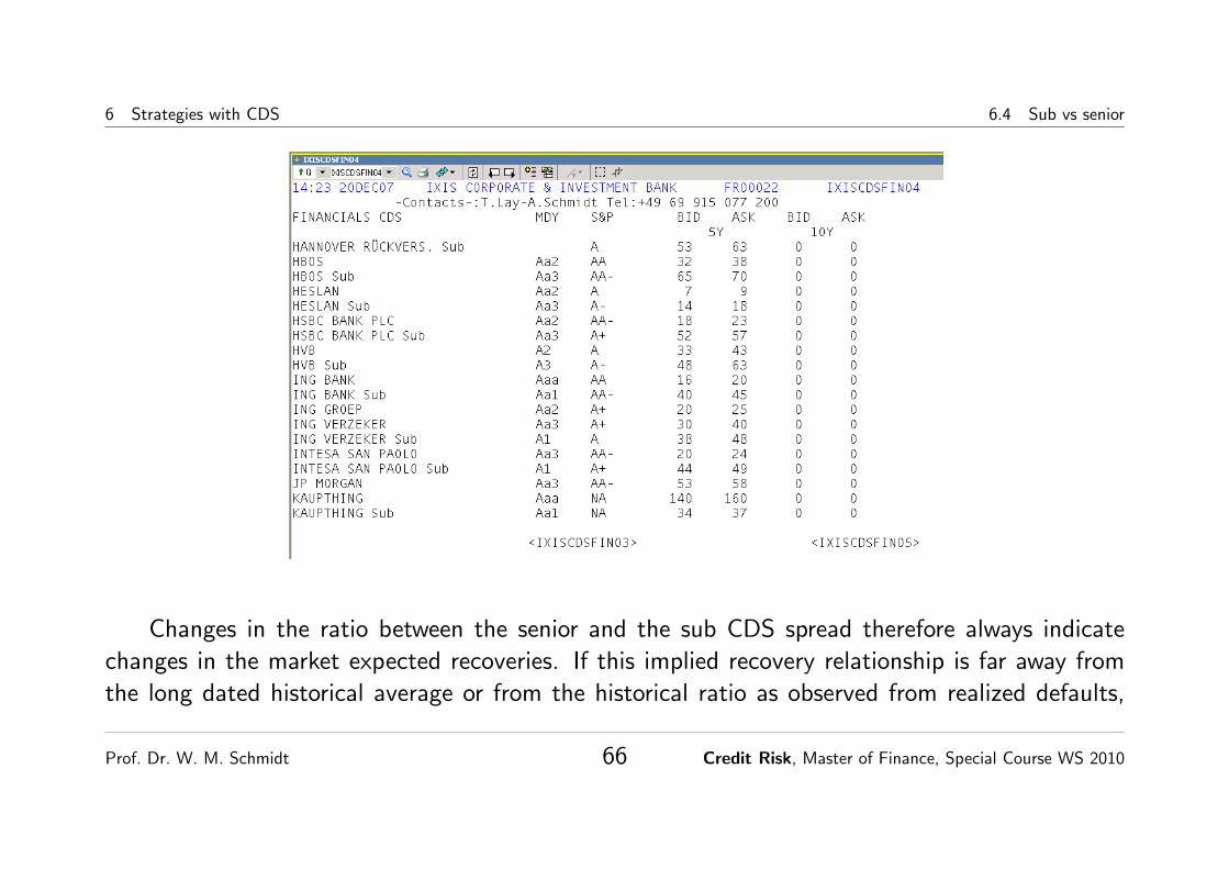
6.4 Sub vs senior
For European banks and insurance companies the market quotes at the same time CDS referring
to senior and subordinated debt. By definition both debt classes will default at the same time.
Different CDS premiums for senior and subordinated reflect different expectations on the recovery
rate.
Prof. Dr. W. M. Schmidt 65 Credit Risk, Master of Finance, Special Course WS 2010
6 Strategies with CDS 6.4 Sub vs senior
Changes in the ratio between the senior and the sub CDS spread therefore always indicate
changes in the market expected recoveries. If this implied recovery relationship is far away from
the long dated historical average or from the historical ratio as observed from realized defaults,
Prof. Dr. W. M. Schmidt 66 Credit Risk, Master of Finance, Special Course WS 2010

6 Strategies with CDS 6.4 Sub vs senior
this might give the opportunity to implement relative value strategies.
Based on the formula (7) we get the following theoretical relationship between the spreads
and the expected recovery ratessCDSsen
sCDSsub=
1− Rsen
1− Rsub.
Prof. Dr. W. M. Schmidt 67 Credit Risk, Master of Finance, Special Course WS 2010
7 Default modeling
7 Default modeling
To evaluate a default risky position, e.g., a CDS or a bond, so far we have only used the CDS
curve of survival probabilities. There was no need for a complicated valuation model. However,
for more complex products such as options or correlation products we need a stochastic model
describing the default and the evolution of the spreads over time. Clearly such a model has to be
in line with the observed market information, primarily the CDS curve, i.e., the model has to be
calibrated to match the given CDS curve.
Observe again the analogy to interest rate models: to evaluate bonds, swaps or FRAs all that
is needed is the discount curve. More complex products require a term structure model which has
to be calibrated to the interest rate curve.
Prof. Dr. W. M. Schmidt 68 Credit Risk, Master of Finance, Special Course WS 2010

7 Default modeling 7.1 Default intensity, hazard rate out of today
7.1 Default intensity, hazard rate out of today
The valuation of any credit derivative product is based on the curve of risk-neutral survival
probabilities derived from actual market data (CDS spreads, prices of bonds).
Let τ denote again the random time of default. Then
F (t) = P(τ < t), t ≥ 0
is the distribution function of τ , and
q(t) = P(τ ≥ t) = 1− F (t), t ≥ 0,
is the curve of survival probabilities (survival function).
Prof. Dr. W. M. Schmidt 69 Credit Risk, Master of Finance, Special Course WS 2010

7 Default modeling 7.1 Default intensity, hazard rate out of today
The conditional probability of default in the interval [t, t+ ∆], given that there has been no
default until time t is calculated as
P(τ ∈ [t, t+ ∆]|τ > t) =F (t+ ∆)− F (t)
1− F (t)
≈F ′(t)
1− F (t)∆.
Here λ0(t) := F ′(t)1−F (t) is called the hazard rate or default intensity. Intuitively this is just the
default rate per year as of today. Using the default intensity we get
λ0(t) = −q′(t)
q(t)
q(t) = P(τ > t) = exp
(−∫ t
0
λ0(s)ds
). (4)
Prof. Dr. W. M. Schmidt 70 Credit Risk, Master of Finance, Special Course WS 2010

7 Default modeling 7.1 Default intensity, hazard rate out of today
For a constant default intensity λ0(t) = λ this implies an Exponential distribution for the
default time:
q(t) = exp(−λt), (5)
F (t) = 1− exp(−λt). (6)
Under the idealized assumption of
• a flat (constant) zero interest rate curve
• a flat (constant) spread curve
• continuous spread payments (monthly, weekly . . . )
the default intensity can be calculated directly from the spread by the rule of thumb formula
λ =s
1− R(7)
with s the CDS spread on an act/act basis. This formula is also known as the credit triangle.
Prof. Dr. W. M. Schmidt 71 Credit Risk, Master of Finance, Special Course WS 2010
7 Default modeling 7.1 Default intensity, hazard rate out of today
Exercise 7.1. Derive the credit triangle formula (7) under the above mentioned conditions.
In case of a constant default intensity the survival probability q(t) for different time points t1, t2is related by
q(t2) = q(t1)t2t1 .
For example, the 1 year and the 1 month survival probabilities are related by q(1M) = q(1Y )112 .
This translates into a corresponding relationship for default probabilities.
Prof. Dr. W. M. Schmidt 72 Credit Risk, Master of Finance, Special Course WS 2010
7 Default modeling 7.2 Models for the default time
7.2 Models for the default time
There is a variety of modeling approaches for structured interest rate products. These models
describe the uncertain future evolution of the yield curve by modeling the dynamics of zero bonds,
the short rate, forward rates or Libor rates. Modeling is done under the so-called risk-neutral
distribution or any other appropriate martingale measure.
Pricing complex credit derivative products follows similar ideas. In principle one has to come
up with a model which combines a model for the risk-free interest rate term structure with a
model for default.
Finally, the price of a complex product turns out to be the discounted risk-neutral expectation
of its payoff. By no-arbitrage pricing theory this price covers exactly the cost of dynamic
replication (hedging).
Prof. Dr. W. M. Schmidt 73 Credit Risk, Master of Finance, Special Course WS 2010

7 Default modeling 7.2 Models for the default time
7.2.1 Structural models
The default time is modeled explicitly by a so-called asset value process (ability to pay process)
(At). The classical Merton model [Merton, 1974] describes default by the relation
τ < T ⇔ AT < KT
with KT denoting the liability process (threshold, barrier). This models is capable of describing
the default at a fixed time T . The model can be easily generalized to allow for a default at any
time t: the default time is the first hitting time of a (time varying) barrier (Kt)
τ = min{t ≥ 0 : At ≤ Kt},
[Longstaff and Schwartz, 1995].
A structural model has to be calibrated to the market implied default curve q(t) = P(τ > t).
This can be done by specifying the dynamics of (At) or (Kt) appropriately, e.g., by drift
calibration.
Prof. Dr. W. M. Schmidt 74 Credit Risk, Master of Finance, Special Course WS 2010
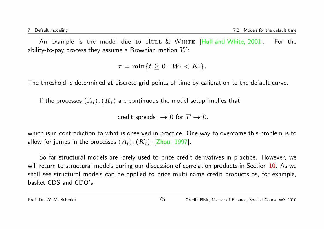
7 Default modeling 7.2 Models for the default time
An example is the model due to Hull & White [Hull and White, 2001]. For the
ability-to-pay process they assume a Brownian motion W :
τ = min{t ≥ 0 : Wt < Kt}.
The threshold is determined at discrete grid points of time by calibration to the default curve.
If the processes (At), (Kt) are continuous the model setup implies that
credit spreads → 0 for T → 0,
which is in contradiction to what is observed in practice. One way to overcome this problem is to
allow for jumps in the processes (At), (Kt), [Zhou, 1997].
So far structural models are rarely used to price credit derivatives in practice. However, we
will return to structural models during our discussion of correlation products in Section 10. As we
shall see structural models can be applied to price multi-name credit products as, for example,
basket CDS and CDO’s.
Prof. Dr. W. M. Schmidt 75 Credit Risk, Master of Finance, Special Course WS 2010

7 Default modeling 7.2 Models for the default time
For further information on structural models we refer to [Bielecki and Rutkowski, 2002],
[Duffie and Singleton, 2003], [Lando, 2004].
7.2.2 Reduced form models
In the framework of a reduced form model the default time τ is modeled only implicitly. There is
no such intuitive representation of the default time as in the framework of structural models. In
the simplest case the default time is just the first jump of a Poisson process with jump intensity
parameter λ. In this case the default time is exponentially distributed with the constant hazard
rate λ.
Clearly, in reality the hazard rate is not constant over time but itself a stochastic process.
This is in line with the fact that credit spreads are not static and stochastically varying over time.
Therefore we start our modeling with a random process (λt) for the hazard rate (default
Prof. Dr. W. M. Schmidt 76 Credit Risk, Master of Finance, Special Course WS 2010
7 Default modeling 7.2 Models for the default time
intensity), e.g., a log-normal process
λt = λ0 exp (σWt + µt) ,
with some Brownian motion W , spread volatility σ and drift µt.
Now, intuitively one can think of the mechanics behind the random default time as follows.
We work on a discrete time scale ∆, 2∆, 3∆, . . . and the default time τ is the result of a series
of the following two-step experiments:
1. start with todays hazard rate λ0 for the interval [0,∆]
2. perform a two outcome (1=success, 0=no success) random experiment (flip a coin) with
probability of success λ0∆. If the outcome is a success this means a default during the interval
[0,∆] and we stop, otherwise
3. sample the hazard rate λ∆ for the interval [∆, 2∆],
4. perform a two outcome random experiment with probability of success λ∆∆. In case of
success we have a default in the interval [∆, 2∆] otherwise . . .
Given a model for the hazard rate process (λt), the distribution of the default time
Prof. Dr. W. M. Schmidt 77 Credit Risk, Master of Finance, Special Course WS 2010
7 Default modeling 7.2 Models for the default time
conditional on the fact that the path of (λt) is known is just,
P(τ > t|σ(λ.)) = exp
(−∫ t
0
λsds
).
That means, conditionally on the knowledge of (λt) the default time possesses a kind of
exponential distribution with time dependent parameter λt, compare this with (4). On a
computer one would simulate the default time by first simulating a path of (λt) and then
generate τ from
τ = min
{t ≥ 0 : exp
(−∫ t
0
λudu
)≤ U
},
where U is a [0, 1] uniform random outcome. In this respect the default time τ is again a first
hitting time of a threshold – observe the surprising analogy to structural models!
A key result for applying reduced form models for the pricing of credit derivatives is the
following.
The price today V0(X1{τ>T}) of a default risky product with payoff X at time T if there is
Prof. Dr. W. M. Schmidt 78 Credit Risk, Master of Finance, Special Course WS 2010

7 Default modeling 7.2 Models for the default time
no default is by the general theory the risk-neutral expectation, which can be calculated as
V0(X1{τ>T}) = E(e−∫ T0 rsdsX1{τ>T}
)= E
(e−∫ T0 (rs+λs)dsX
).
This means that λt can be interpreted as continuously compounded spread over the risk free
short rate rt. This observation is the main reason for fruitful similarities to interest rate term
structure modeling, which in turn explains why modelers and practitioners are in favor of reduced
form models.
For further reading on reduced form models we refer to [Bielecki and Rutkowski, 2002],
[Duffie and Singleton, 2003], [Lando, 2004], [Schonbucher, 2003].
To implement the model in practice one has to take care of at least two factors, the default
free interest rate term structure and the term structure of default probabilities. In the simplest
approach one combines a 1-factor short rate model with a 1-factor model for the default intensity
(λt).
Prof. Dr. W. M. Schmidt 79 Credit Risk, Master of Finance, Special Course WS 2010

8 CDS Indices
8 CDS Indices
Soon after the market in credit derivatives turned into a quite developed market participants
initiated the design of various credit indices which are nowadays traded with excellent liquidity
and, as such, allow for a variety of investment strategies.
The 2001 founded International Index Company (IIC) is administrating and managing the
roll out of the so-called ITraxx credit indices and the ibex bond indices. The company Markit
(www.markit.com) is in charge of independent pricing.
We are focusing on the European index family DJ iTraxx Europe. There exist an overall
benchmark index and several sector indices. The indices are available in CDS format (unfunded)
as well as in CLN format (funded). On top of those indices there are standardized tranches on the
index baskets and first-to-default basket default swaps on the sectors. As we shall understand,
this wide spectrum of standardized highly liquid instruments allows for cross asset class strategies
and an active trading of correlation.
Prof. Dr. W. M. Schmidt 80 Credit Risk, Master of Finance, Special Course WS 2010

8 CDS Indices
6
Comprehensive European platform
iTraxx Europe, HiVol
5 and 10
iTraxx CrossOver
Benchmark indices Standard maturities
Exposure to 45 Europeansub-investment grade
reference entities
iTraxx Europe Crossover
Top 125 names in terms ofCDS volume traded in the six
months prior to the roll
iTraxx Europe
TMT
20 enities
Energy
30 entities
20 entities
Industrials
Consumers
25 entities
Financials Senior
25 entities
Financials Sub
Autos
100 entities
Non-Financials
Top 30 highest spread names from iTraxx Europe
iTraxx Europe HiVol
Sector indices
First to Default baskets:Autos, Consumer, Energy, Financial (sen / sub), Industrials, TMT, HiVol, Crossover, Diversified
3
5
7
10
5 and 10
iTraxx Sector Indices
10 entities20 entities
Prof. Dr. W. M. Schmidt 81 Credit Risk, Master of Finance, Special Course WS 2010

8 CDS Indices
A new series of the indices is rolled out every 6 months on March 20 and September 20. The
constituents of the index are equally weighted with time to maturity of mainly 5 and 10 years.
For protection buyers the index provides a macro hedge.
At a first glance the iTraxx index swap looks like a plain portfolio of CDS. However, the
spread of the index as determined at the time of roll out stays unchanged during the life time of
the index and any changes in credit quality are compensated by an upfront price charge when
buying/selling the index.
The initially agreed spread is paid on regularly on a quarterly, act/360 basis in each period
referring to the outstanding notional amount of the index basket. Whenever a default in the
index occurs, the notional of the index is reduced by the respective percentage amount, e.g., 5%
in case of the iTraxx Europe Energy. If the index is in CLN format as a consequence of a default
in the basket the redemption of the note at maturity is reduced by the corresponding percentage
x% and there is an early redemption of R · x% of the notional with R denoting the recovery
rate of the defaulted name.
Prof. Dr. W. M. Schmidt 82 Credit Risk, Master of Finance, Special Course WS 2010

8 CDS Indices
Prof. Dr. W. M. Schmidt 83 Credit Risk, Master of Finance, Special Course WS 2010

8 CDS Indices
Since the spread for the index stays unchanged during its life, any change in credit worthiness of
the underlying names has to be compensated by an upfront fee when buying/selling the index.
The market quotes actual index spreads which allow for a simple calculation of this upfront
charge. Referring the quotes above, the 10Y index is quoted at 131.9 bps whereas the contract
spread is 100 bps. Now the upfront payment is calculated as if one determines the mark-to-market
value of a 100 bps CDS priced on a flat curve of 131.9 bps and assuming a recovery of 40%.
Since all names in the index are equally weighted it seems that the theoretically fair spread
for the index at inception is just the average of the CDS spread of all names in the index. Why is
this not correct and how should the fair spread of the index be calculated?
Prof. Dr. W. M. Schmidt 84 Credit Risk, Master of Finance, Special Course WS 2010

9 Correlation products
9 Correlation products
9.1 Basket Default Swaps
A basket default swap is like a plain credit default swap but refers to a whole basket of n
reference names (underlyings). A kth-to-default swap provides insurance against the event of the
kth default out of the underlying n names. An insurance premium, the kth-to-default spread,
skth is paid to the protection seller. In return the protection buyer gets compensated for the loss
caused by the kth default if this occurs before maturity. Most popular are first-to-default swaps
(FTD).
Motivation: A first-to-default swap on n (usually 3-7) names yields an extremely attractive
premium income for the investor selling protection.
Prof. Dr. W. M. Schmidt 85 Credit Risk, Master of Finance, Special Course WS 2010

9 Correlation products 9.1 Basket Default Swaps
protection seller protection buyer
�
-
-
-yes: compensation for loss
no: payment = 0
premium paid until maturity or credit event
credit event6
reference basket
Prof. Dr. W. M. Schmidt 86 Credit Risk, Master of Finance, Special Course WS 2010

9 Correlation products 9.1 Basket Default Swaps
Valuation
• depends clearly on the credit quality of the single names in the basket;
• the fair FTD spread (insurance premium) is between the maximum of all spreads in the basket
and their sum;
• depends on the strength of “dependencies” between the names in the basket:
– for a correlation close to zero, the fair FTD spread is about the sum of all spreads in the
basket (explain why!),
– for a correlation close to 1 the fair FTD spread is close to the widest spread in the basket.
– as a rule of thumb: the fair FTD spread is, depending on correlation, about 40% to 75%
of the sum of all spreads.
The more diversified the basket, the higher is the FTD premium which has to be received by
the protection seller. A basket with relatively homogeneous spreads is preferable since otherwise
the name with the widest spread will dominate the basket.
Prof. Dr. W. M. Schmidt 87 Credit Risk, Master of Finance, Special Course WS 2010
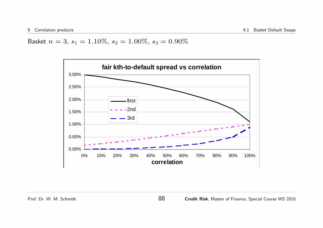
9 Correlation products 9.1 Basket Default Swaps
Basket n = 3, s1 = 1.10%, s2 = 1.00%, s3 = 0.90%
fair kth-to-default spread vs correlation
0.00%
0.50%
1.00%
1.50%
2.00%
2.50%
3.00%
0% 10% 20% 30% 40% 50% 60% 70% 80% 90% 100%
correlation
first
2nd
3rd
Prof. Dr. W. M. Schmidt 88 Credit Risk, Master of Finance, Special Course WS 2010
9 Correlation products 9.2 CDO Tranches
9.2 CDO Tranches
A (synthetic) CDO is based on a portfolio (pool) of n underlying default risks. Often the pool
is synthetically created by selling protection on the names in the pool via CDS. The default
risk (loss) of the portfolio is divided into slices, so-called tranches, and these risks are finally
securitized. The lowest tranche, the junior or equity tranche, takes the first losses occurring from
defaults in the pool. Further losses, exceeding the size of the equity tranche are covered by the
next tranche (mezzanine tranche), and so on. The investor buying a note on the tranche receives
a spread as compensation for the risk he has taken on.
The valuation of the tranches
• depends on the credit quality (spreads) of the individual names in the pool,
• depends on the strength of “dependencies” between the names in the pool.
To illustrate the last point we show below the loss distribution for various correlations and for a
pool with n = 100, s = 1.00%, R = 40%.
Prof. Dr. W. M. Schmidt 89 Credit Risk, Master of Finance, Special Course WS 2010
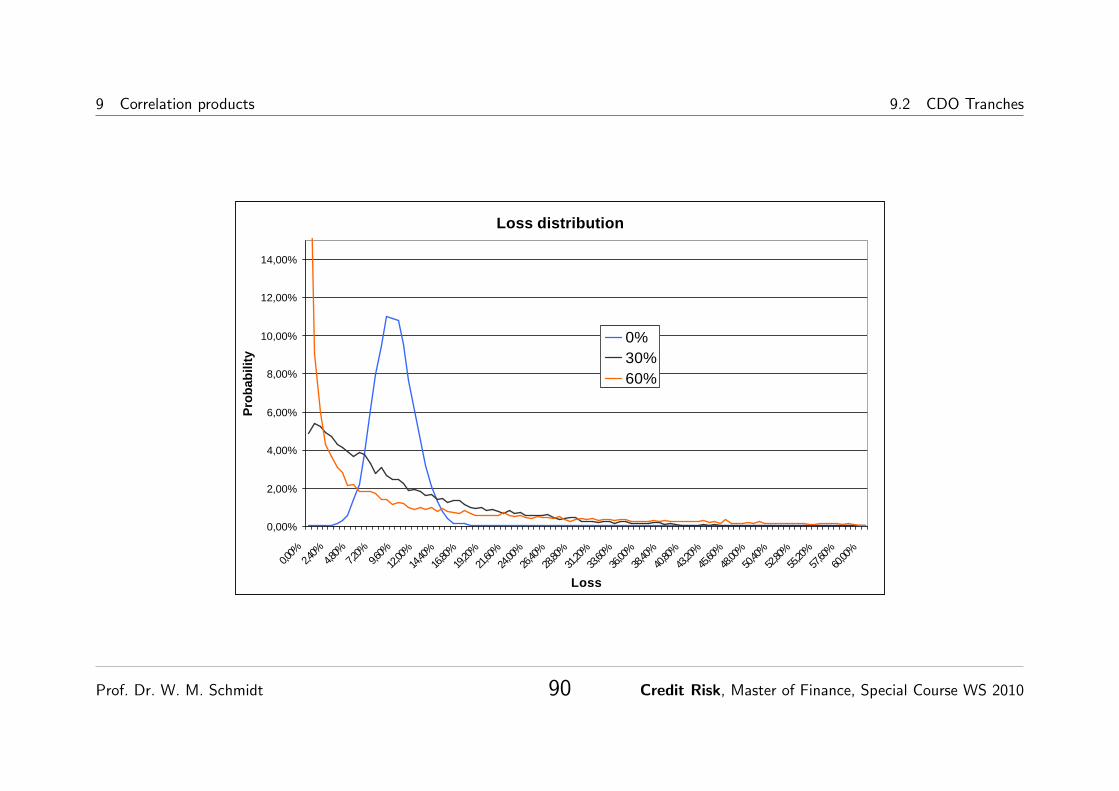
9 Correlation products 9.2 CDO Tranches
Loss distribution
0,00%
2,00%
4,00%
6,00%
8,00%
10,00%
12,00%
14,00%
0,00%
2,40%
4,80%
7,20%
9,60%
12,00
%14
,40%
16,80
%19
,20%
21,60
%24
,00%
26,40
%28
,80%
31,20
%33
,60%
36,00
%38
,40%
40,80
%43
,20%
45,60
%48
,00%
50,40
%52
,80%
55,20
%57
,60%
60,00
%
Loss
Pro
babi
lity
0%30%60%
Prof. Dr. W. M. Schmidt 90 Credit Risk, Master of Finance, Special Course WS 2010

9 Correlation products 9.3 Synthetic CDO tranches on the benchmark index
Selected default probabilitiesnumber of defaults /correlation 0% 30% 60%
> 1 100,00% 89,82% 66,13%
> 10 91,70% 51,57% 38,52%
> 20 8,02% 27,29% 26,06%
9.3 Synthetic CDO tranches on the benchmark index
Based on the iTraxx Europe benchmark index the following standardized tranches are traded:
tranche range of loss
Equity 0-3%
BBB 3-6%
AAA 6-9%
Junior Super Senior Low 9-12%
Junior Super Senior High 12-22%
Investment Grade 3-100%
Prof. Dr. W. M. Schmidt 91 Credit Risk, Master of Finance, Special Course WS 2010

9 Correlation products 9.3 Synthetic CDO tranches on the benchmark index
All tranches above the equity tranche are quoted by their fair spread. The quotes for the
equity tranche always assume a running spread of 500 bps and any remaining difference in value
between the premium leg and the protection leg is compensated by ab upfront charge.
Determining the price of a tranche is quite complex. The price depends on the spreads of
the names in the underlying portfolio, assumptions about their recoveries and, most importantly,
on their correlation. Nowadays tranches are sometimes quoted by their implied correlationassuming a 1-factor Gaussian copula model (similar to the Basel II model). The tranche market
is therefore mainly a correlation market.
The individual tranches react quite differently to changes of the correlation.
Prof. Dr. W. M. Schmidt 92 Credit Risk, Master of Finance, Special Course WS 2010

9 Correlation products 9.3 Synthetic CDO tranches on the benchmark index
52
Global Markets ResearchEuropean Credit Strategy
Kreditderivate Spezial - Das Sahnehäubchen im Kreditmarkt07. 02. 2005
©HVB Corporates & Markets, Global Markets Research.See third to last page for disclaimer.
in Bezug auf das Korrelationsrisiko reagieren.
Eine höhere Korrelationverändert die Verlustallokationder Tranchen, während dererwartete Verlust des Basketsunverändert bleibt
Wir haben bereits erarbeitet, welchen Einfluss der Korrelationsparameter aufdie Verlustverteilung des zugrundeliegenden Baskets ausübt. Auch wenn eineVariation des Korrelationsparameters keinen Einfluss auf den erwartetenVerlust des zugrundeliegenden Baskets besitzt, ändert sich jedoch die Gestaltder Verlustverteilung. Eine Erhöhung der Korrelation läßt die Randbereiche derVerlustverteilung zu Lasten der “Mitte” anwachsen. Szenarien, in denen keineoder sehr viele Ausfälle resultieren, werden wahrscheinlicher. Obwohl dererwartete Verlust des zugrundeliegenden Baskets unverändert bleibt, ändertsich also die Verlustallokation für die einzelnen Tranchen.
W I E D J I T R A X X - T R A N C H E N A U F E I N E V E R Ä N D E R U N G D E R K O R R E L A T I O N R E A G I E R E N
-0.6
-0.4
-0.2
0.0
0.2
0.4
0.6
0% 10% 20% 30% 40% 50% 60% 70% 80% 90% 100%Korrelationsparameter
Barw
ert
än
deru
ng
(in
% d
es
No
min
als
)
EquityBBBAAAJuniorSenior
0
1000
2000
3000
4000
0% 10% 20% 30% 40% 50% 60% 70% 80% 90% 100%Korrelationsparameter
Fair
es
Sp
read
niv
eau
(in
bp
)
EquityBBBAAAJuniorSenior
Quelle: HVB Global Markets Research
Veränderungen von Spreadsbzw. Barwerten ist fürMezzanine-Tranchen wenigeingängig
Da eine höhere Korrelation fettere Ränder der Verlustverteilung impliziert,würde man erwarten, dass sich das faire Spreadniveau einer Equity-Trancheaufgrund der erhöhten Wahrscheinlichkeit für keine (bzw. sehr wenige) Verlustereduziert. Auf der anderen Seite sollte der faire Spread einer Senior-Trancheansteigen, da Szenarien mit gehäuften Ausfällen wahrscheinlicher werden.Beide obigen Abbildungen bestätigen, dass die Equity-Tranche die höchsteSensitivität bzgl. des Korrelationsparameters aufweist. Jedoch ist dieWirkungsrichtung für Mezzanine-Tranchern weniger eingängig. DieAbbildungen offenbaren Wertebereiche mit steigenden Spreads, aber auchwelche mit sinkenden Spreads.
D I E S E N S I T I V I T Ä T B E Z Ü G L I C H D E R R E C O V E R Y - Q U O T E
Die erwartete Recovery-Quoteist ein Risikofaktor, der allzugerne als gegeben angesehenwird
Schließlich fehlt noch eine Analyse, wie die Veränderung der einheitlichenRecovery-Quote die DJ iTrax-Tranchen beeinflusst. Die Marktkonvention fürdie Recovery-Quote in Höhe von 40% wird üblicherweise als gegebenangesehen, wohingegen uns die Realität häufig eines Besseren belehrt.Deshalb sollte man sich als Investor klar machen, dass die erwarteteRecovery-Quote ein weiterer wichtiger Marktrisikofaktor darstellt.
Wie zuvor stellen wir dieBewertungsänderung vonbereits existierenden Tranchenund deren fairenSpreadniveaus dar
Im vorliegenden Abschnitt stellen wir analog zu den anderen Risikofaktorenheraus, wie Erwartungsveränderungen bzgl. der Recovery-Quote den Barwertvon bereits existierenden DJ iTraxx-Tranchen und deren fairen Spreadniveausbeeinflussen. Die folgenden Abbildungen zeigen eindrucksvoll, welchen Einflussunterschiedliche Recovery-Quoten (0% - 100%) aufweisen, wobei die Equity-
Increasing the correlation, the risk of joint defaults increases. This implies that the spread
of the tranches with hight subordination, the senior tranches, is widening. On the other hand,
Prof. Dr. W. M. Schmidt 93 Credit Risk, Master of Finance, Special Course WS 2010
10 What is default correlation?
a higher correlation also increases the chances if many joint survivals which leads to a tighter
spread on the equity tranche. For the mezzanine tranches the picture is not that clear - often the
spread initially increases with correlation but later decreases when correlation further increases.
10 What is default correlation?
Modeling defaults in principle involves two tasks
• modeling the random time of default τ ,
• modeling the random severity of the loss L.
Speaking about default correlation it is not obvious what kind of correlation that should be.
Prof. Dr. W. M. Schmidt 94 Credit Risk, Master of Finance, Special Course WS 2010
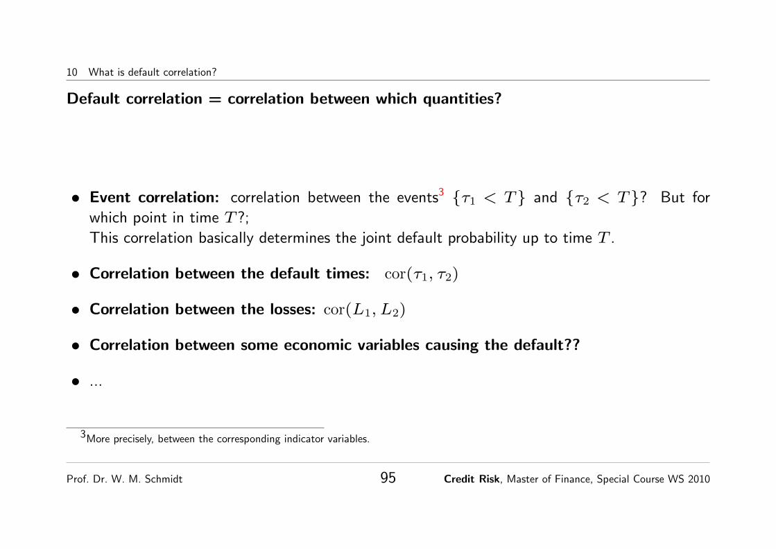
10 What is default correlation?
Default correlation = correlation between which quantities?
• Event correlation: correlation between the events3 {τ1 < T} and {τ2 < T}? But for
which point in time T ?;
This correlation basically determines the joint default probability up to time T .
• Correlation between the default times: cor(τ1, τ2)
• Correlation between the losses: cor(L1, L2)
• Correlation between some economic variables causing the default??
• ...
3More precisely, between the corresponding indicator variables.
Prof. Dr. W. M. Schmidt 95 Credit Risk, Master of Finance, Special Course WS 2010

10 What is default correlation? 10.1 Event correlation
10.1 Event correlation
The default event correlation ρE(T ) between two names and for the time horizon T is defined as
ρE
(T ) = cor(1{τ1<T}, 1{τ2<T}). (8)
In other words, the probability of a joint default is
P(τ1 < T, τ2 < T ) = F1(T )F2(T ) + ρE
(T )√F1(T )(1− F1(T ))F2(T )(1− F2(T ))
F1(T ) = P(τ1 < T )
F2(T ) = P(τ2 < T ).
In view of 0 ≤ P(τ1 < T, τ2 < T ) ≤ min(F1(T ), F2(T )), the default correlation is bounded
by the following natural bounds
−F1(T )F2(T )√F1(T )(1− F1(T ))F2(T )(1− F2(T ))
≤ ρE(T ) ≤
√u(1− v)
v(1− u),
Prof. Dr. W. M. Schmidt 96 Credit Risk, Master of Finance, Special Course WS 2010

10 What is default correlation? 10.2 Asset correlation
where u = min(F1(T ), F2(T )) and v = max(F1(T ), F2(T )).
Compared to the so-called asset correlation to be introduced in the next section, the event
correlation takes much smaller values.
10.2 Asset correlation
Out of the two fundamental approaches to default modeling, as discussed in Section 7.2, the
structural approach is particularly well suited to be extended to model dependent defaults.
Denote by (At) the value of the assets of the underlying firm (asset value process) and by
(Kt) the value of its liabilities at time t. The difference Pt = At −Kt is sometimes called
the ability-to-pay process. In the framework of the Merton model one considers a fixed time
horizon T and the firm is in default if and only if PT < 0. Usually Kt is assumed to be a
constant whereas (At) follows a Black & Scholes type model, a geometric Brownian motion.
In this case the variable PT can be transformed into a standard normal variable Y and the
Prof. Dr. W. M. Schmidt 97 Credit Risk, Master of Finance, Special Course WS 2010

10 What is default correlation? 10.2 Asset correlation
default event for time T reduces to
{τ < T} = {Y < c},
where the constant c is the so-called distance to default. With N denoting the standard normal
distribution function we obtain
F (T ) = P(τ < T ) = P(Y < c) = N(c),
and the distance to default is related to the default probability by
c = N(−1)
(F (T ))4. (9)
Now consider n default risky entities whose default times are denoted by τ1, . . . , τn. For
each underlying name i we assume a Merton model with standard normal state variable Yi4For an increasing function G we write G(−1) for its inverse.
Prof. Dr. W. M. Schmidt 98 Credit Risk, Master of Finance, Special Course WS 2010

10 What is default correlation? 10.2 Asset correlation
controlling the default of i. Dependencies between defaults can be modeled easily assuming that
the state variables (Y1, . . . , Yn) are correlated:
ρAi,j(T ) = cor(Yi, Yj). (10)
The correlation ρAi,j(T ) is called the asset correlation (for time horizon T ). The pairwise joint
default probability is now obtained from
P(τi < T, τj < T ) = P(Yi < ci, Yj < cj)
= N2(ci, cj; ρAi,j(T ))
= N2(N(−1)
(Fi(T )),N(−1)
(Fj(T )); ρAi,j(T )). (11)
We will come back to this relationship in Section 11.3.
In the classical Merton model, default is exclusively modeled for the interval up to time T ,
i.e., the model is not able to give the precise term structure of defaults. One can overcome this
Prof. Dr. W. M. Schmidt 99 Credit Risk, Master of Finance, Special Course WS 2010
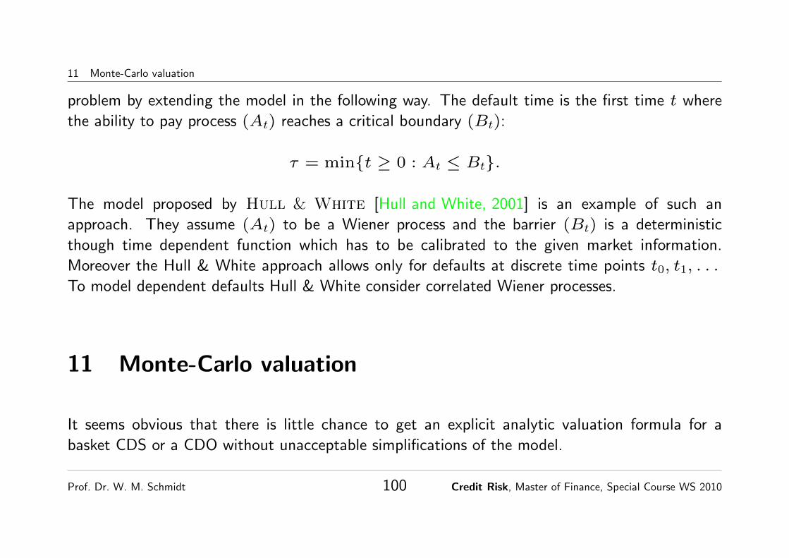
11 Monte-Carlo valuation
problem by extending the model in the following way. The default time is the first time t where
the ability to pay process (At) reaches a critical boundary (Bt):
τ = min{t ≥ 0 : At ≤ Bt}.
The model proposed by Hull & White [Hull and White, 2001] is an example of such an
approach. They assume (At) to be a Wiener process and the barrier (Bt) is a deterministic
though time dependent function which has to be calibrated to the given market information.
Moreover the Hull & White approach allows only for defaults at discrete time points t0, t1, . . .
To model dependent defaults Hull & White consider correlated Wiener processes.
11 Monte-Carlo valuation
It seems obvious that there is little chance to get an explicit analytic valuation formula for a
basket CDS or a CDO without unacceptable simplifications of the model.
Prof. Dr. W. M. Schmidt 100 Credit Risk, Master of Finance, Special Course WS 2010

11 Monte-Carlo valuation 11.1 How to simulate default times?
In practice the valuation is therefore mainly done via a Monte-Carlo simulation for the default
times of the underlying names taking into account their dependencies.
11.1 How to simulate default times?
From the market data (e.g. the CDS spreads) we already derived the distribution function
F (t) = P(τ < t) of the default time τ which is the primary input to any valuation model. How
to Monte-Carlo simulate samples of a default time τ whose distribution function F is given?
A simple fact from probability calculus states that
U = F (τ) (12)
possesses a uniform distribution on [0, 1]. Vice versa, the random variable τ generated by the
rule 5
τ = F(−1)
(U) (13)5F (−1) is the inverse to F .
Prof. Dr. W. M. Schmidt 101 Credit Risk, Master of Finance, Special Course WS 2010
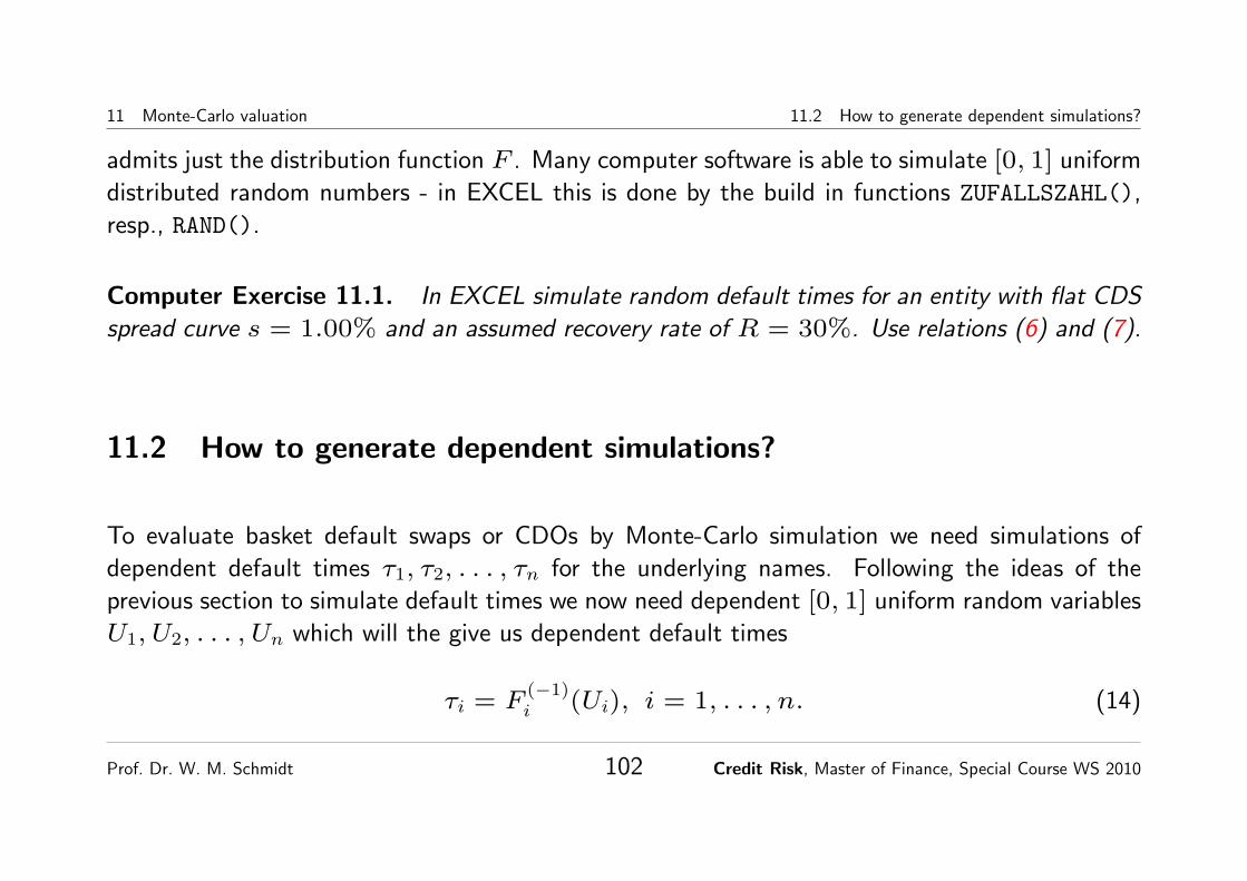
11 Monte-Carlo valuation 11.2 How to generate dependent simulations?
admits just the distribution function F . Many computer software is able to simulate [0, 1] uniform
distributed random numbers - in EXCEL this is done by the build in functions ZUFALLSZAHL(),
resp., RAND().
Computer Exercise 11.1. In EXCEL simulate random default times for an entity with flat CDS
spread curve s = 1.00% and an assumed recovery rate of R = 30%. Use relations (6) and (7).
11.2 How to generate dependent simulations?
To evaluate basket default swaps or CDOs by Monte-Carlo simulation we need simulations of
dependent default times τ1, τ2, . . . , τn for the underlying names. Following the ideas of the
previous section to simulate default times we now need dependent [0, 1] uniform random variables
U1, U2, . . . , Un which will the give us dependent default times
τi = F(−1)i (Ui), i = 1, . . . , n. (14)
Prof. Dr. W. M. Schmidt 102 Credit Risk, Master of Finance, Special Course WS 2010

11 Monte-Carlo valuation 11.2 How to generate dependent simulations?
Generating dependent uniforms U1, . . . , Un is not as straightforward as it seems. On the
other hand, it is quite easy to generate correlated standard normals Y1, Y2, . . . , Yn with some
given correlation matrix Σ. But why don’t we use those to derive also dependent uniforms
U1, U2, . . . , Un and thus dependent default times τ1, τ2, . . . , τn applying the transformations
(see (12)!)
Ui = N(Yi) (15)
τi = F(−1)i (Ui) = F
(−1)i (N(Yi)) (16)
with N denoting the standard normal distribution function.
Recall how correlated standard normal variables with a given correlation matrix can be
generated. We have to start with independent standard normals and combine them linearly by
multiplication with the Cholesky decomposition of the correlation matrix. For n = 2 things
simplify and for a given correlation of ρ correlated normals Y1, Y2 are derived from independent
ones X1, X2 simply by
Y1 = X1, Y2 = ρ X1 +√
1− ρ2 X2.
Prof. Dr. W. M. Schmidt 103 Credit Risk, Master of Finance, Special Course WS 2010

11 Monte-Carlo valuation 11.3 Normal copula and asset correlation
Computer Exercise 11.2. In EXCEL simulate dependent default times τ1, τ2 for a correlation
ρ = 60%, flat CDS curves s1 = 1.00%, s2 = 1.50% and recovery rates R1 = R2 = 40%.
What happens when the correlation approaches 100%?
11.3 Normal copula and asset correlation
Generating dependent default times following the approach from the previous section needs some
critical review. What role is played by the normal distribution there which was just a tool to
generate dependencies? How to interpret intuitively the correlation matrix Σ there? Are there
alternative, possibly better suited approaches?
The dependent standard normals Y1, Y2, . . . , Yn in the previous section are distributed with
joint distribution function
P(Y1 < y1, Y2 < y2, . . . , Yn < yn) = N(y1, y2, . . . , yn; Σ).
Prof. Dr. W. M. Schmidt 104 Credit Risk, Master of Finance, Special Course WS 2010

11 Monte-Carlo valuation 11.3 Normal copula and asset correlation
Applying the transformation Ui = N(Yi) the somehow(!) dependent uniforms are jointly
distributed according to
P(U1 < u1, U2 < u2, . . . , Un < un)
= P(Y1 < N(−1)
(u1), Y2 < N(−1)
(u2), . . . , Yn < N(−1)
(un))
= N(N(−1)
(u1),N(−1)
(u2), . . .N(−1)
(un); Σ)
=: C(u1, u2, . . . , un).
The function C(u1, u2, . . . , un) describes the joint distribution of dependent uniforms. Such a
function C is called a Copula, and in the special case above it is the so-called Normal Copula.
The joint distribution of the constructed default times τ1, τ2, . . . , τn can be written as
P(τ1 < t1, τ2 < t2, . . . , τn < tn)
= C(F1(t1), F2(t2), . . . , Fn(tn)). (17)
Here the joint distribution appears as the marginal distributions F1, . . . , Fn linked by the
Prof. Dr. W. M. Schmidt 105 Credit Risk, Master of Finance, Special Course WS 2010

11 Monte-Carlo valuation 11.3 Normal copula and asset correlation
copula C which defines the dependencies. The copula links the marginal distributions into
a joint distribution. Any kind of dependence can be modeled through an appropriate copula
and any joint distribution has some copula in the background. Copulas allow for much richer
dependencies as compared to correlation which is just a measure of linear dependence. We refer
to [Embrechts et al., 1999], [Nelsen, 1999] for further reading.
Currently copulas are getting more and more popular in risk manage-
ment, and, in particular, in the area of dependent credit risks, see e.g.
[Frey et al., 2001],[Li, 2000],[Schmidt and Ward, 2002].
What is left is an intuitive interpretation of the correlation Σ = (ρij) used in our normal
copula approach. The pairwise joint probabilities of default until time T are
P(τi < T, τj < T ) = P(F(−1)i (N(Yi)) < T, F
(−1)j (N(Yj)) < T )
= P(Yi < N(−1)
(Fi(T )), Yj < N(−1)
(Fj(T )))
= N2(N(−1)
(Fi(T )),N(−1)
(Fj(T )), ρij)
Prof. Dr. W. M. Schmidt 106 Credit Risk, Master of Finance, Special Course WS 2010

11 Monte-Carlo valuation 11.4 Pricing basket CDS
and comparing them with relation (11) shows immediately that the correlation ρij is nothing
else but the asset correlation ρaij(T ) in the multi credit extension of the Merton model! The
correlations in the normal copula approach to dependent default are just asset correlations!
11.4 Pricing basket CDS
To evaluate a first-to-default swap we have to investigate the time
τmin = min(τ1, τ2, . . . , τn)
of the first default. Once we know the survival probability curve for τmin,
qmin(t) = P(τmin ≥ t) = P(τ1 ≥ t, τ2 ≥ t, . . . , τn ≥ t)
a FTD basket can be valued exactly as a plain-vanilla CDS, we only have to replace in formula (3)
the survival curve q(t) by qmin(t). However, this would assume that all names in the underlying
basket possess one and the same recovery rate.
Prof. Dr. W. M. Schmidt 107 Credit Risk, Master of Finance, Special Course WS 2010

11 Monte-Carlo valuation 11.4 Pricing basket CDS
Simulating the default times τ1, τ2, . . . , τn and thus τmin, one can calculate the survival
probabilities qmin(t) empirically by estimation from the simulations.
Computer Exercise 11.3. Price an FTD basket CDS with n = 3 names, flat individual CDS
curves s1 = 1.10%, s2 = 1.00%, s3 = 0.90% and a time to maturity of T = 5Y (spreadsheet
FTDPricer.xls). We assume a recovery rate of 40% for all names. Play around with the asset
correlation ρ. What is the fair FTD spread obtained for ρ = 100% and for ρ = 0%?
How the sheet FTDPricer.xls works
• Default times are simulated as in Exercise 11.1 and 11.2 following the normal copula approach
(worksheet Valuation columns C to K).
• For the simulation a constant default intensity according to formula (7) is assumed.
Prof. Dr. W. M. Schmidt 108 Credit Risk, Master of Finance, Special Course WS 2010

11 Monte-Carlo valuation 11.4 Pricing basket CDS
• The last term in the valuation formula (3),
FTDExpectedPVLoss =
n∑i=1
E((1− Ri)DF(τmin)1{τmin=τi,τmin≤T}
),
is calculated in a VBA macro and returned in cell R34.
• Riskless discount factors are calculated from the given interest rates by the formula
DF(t) = exp(−rt t),
i.e., the input rates are continuously compounded zero rates on an act/act basis.
• The fair FTD spread sfirst is determined iteratively from the equality
sfirst
RiskyPV01 = FTDExpectedPVLoss.
Prof. Dr. W. M. Schmidt 109 Credit Risk, Master of Finance, Special Course WS 2010

11 Monte-Carlo valuation 11.5 Pricing tranches of CDOs
Here RiskyPV01 is calculated in reasonable approximation by
RiskyPV01 =1
rT + λmin
[1− exp(−(rT + λmin)T )]
λmin =sfirst
1− Raverage
.
11.5 Pricing tranches of CDOs
Pricing tranches of a CDO transaction is clearly much more challenging than pricing an FTD
basket. It is critical to take into account the timing of the individual defaults and the order of
cash flows in default. Similarly to the Monte-Carlo valuation of an FTD one simulates the default
times for the names in the underlying pool. One of the main results of the simulation is the loss
distribution over the pool at maturity of the CDO.
Computer Exercise 11.4. Evaluate the tranches of a CDO referring to a pool of n = 100
names, all with the same flat CDS curve si = 2.00% and recoveries Ri = 40%. The tranche
Prof. Dr. W. M. Schmidt 110 Credit Risk, Master of Finance, Special Course WS 2010

11 Monte-Carlo valuation 11.5 Pricing tranches of CDOs
sizes are sen = 85%,mez = 10%, jun = 5% (spreadsheet CDOPoolPricer.xls). The
maturity of the CDO is T = 5Y . Play around with the asset correlation ρ between the
names. Interpret the results by generating a plot of the loss distribution (worksheet Valuation
P14:Q114).
Prof. Dr. W. M. Schmidt 111 Credit Risk, Master of Finance, Special Course WS 2010

11 Monte-Carlo valuation 11.5 Pricing tranches of CDOs
How the sheet CDOPoolPricer.xls works.
• Default times are simulated as in Exercise 11.1 and 11.2 following the normal copula approach
(worksheet Valuation columns C to J).
• For the simulation a constant default intensity according to formula (7) is assumed.
• The loss distribution at maturity is internally calculated by a VBA macro and shown in
Valuation P14:Q114.
• From that the expected loss for each tranche is calculated in W6:W8. These quantities do
not include timing effects and discounting, they refer to maturity.
• The losses for each tranche are distributed over time according to a fixed schedule
(AB16:AD30) and discounted. The present value PVExpectedLoss per tranche is shown in
AB32:AD32.
• For each tranche the present value of the fair spread payments should compensate for
the PVExpectedLoss. The corresponding fair spreads are determined iteratively where the
recovery has to be adjusted during the calculation of the RiskyPV01 in cells AB9:AD9.
Prof. Dr. W. M. Schmidt 112 Credit Risk, Master of Finance, Special Course WS 2010

Part II
Credit Risk Management
Prof. Dr. W. M. Schmidt 113 Credit Risk, Master of Finance, Special Course WS 2010

12 Credit risk
12 Credit risk
Financial contracts involve at least 2 counter-parties, and the risk that one of the parties does
not fulfill its contractual obligations is called credit risk in widest sense.
In case of credits, loans or fixed income products such as bonds, credit risk is particularly
transparent. Here credit risk accommodates the risk that the borrower or issuer of the bond does
not pay the agreed interest/coupons or does not repay the capital.
However, credit risk is also present in case of investment banking products such as derivatives,
forwards, futures, swaps and options. In that case credit risk involves the risk that one of the
counter-parties does not pay the scheduled cash flows.
Whenever a counter-party does not fulfil its obligations we speak of a default of this
counter-party. For credit derivatives (see Part I) one has to define and formulate exactly
the conditions of a default; for that purpose the ISDA has developed template documents
([International Swap and Derivatives Association, 2003]).
Prof. Dr. W. M. Schmidt 114 Credit Risk, Master of Finance, Special Course WS 2010

12 Credit risk
Credit risk is measured, for example, by rating agencies by so-called ratings. Big agencies
such as Moody’s, Standard & Poor’s or Fitch IBCA have created own, but to a large extent,
comparable systems of ratings. Here is the Standard & Poor’s system:
AAA best credit quality, extremely reliable with regard to financial obligations
AA very good credit quality, very reliable
A more susceptible to economic conditions, still good credit quality
BBB lowest rating in investment grade
BB caution is necessary, best sub-investment credit quality
B vulnerable to changes in economic conditions, currently showing the ability to meet its financialobligations
CCC currently vulnerable to nonpayment, dependent on favorable economic conditions
CC highly vulnerable to a payment default
C close to or already bankrupt, payments on the obligations currently continued
D payment default on some financial obligation has actually occurred
In the meantime many banks have developed their own rating system, which is used to qualify
the credit risk even of quite small counter parties.
For capital market products actively traded in the market, such as, bonds, credit risk is
Prof. Dr. W. M. Schmidt 115 Credit Risk, Master of Finance, Special Course WS 2010

12 Credit risk
reflected in the market price of the instrument. Often, credit risk is quantified by a spreadrelative to a certain benchmark. Contrary to ratings, spreads quantify the risk on a continuous
scale.
Computer Exercise 12.1. A 10Y corporate bond with annual coupon of 5% trades at a market
price (dirty price) of 90,91. A government bond with the same contract specifications trades at
92,64. Using EXCEL determine the yield spread of the corporate bond relative to the benchmark
government.
Exercise 12.2. In practice spreads are not exclusively due to credit risk. Which other components
might enter into market spreads?
Usually credit risk and its impact on the value of a contract is divided into two risk
components: default risk also called event risk, which describes effects caused by a realized
default, and, spread risk or credit quality risk, which is the impact due to changes in credit
quality except default.
Prof. Dr. W. M. Schmidt 116 Credit Risk, Master of Finance, Special Course WS 2010
13 Modeling default
13 Modeling default
Considering a financial contract, we are going to formalize the inherent credit risk. Due to a
default by the counter party the owner of the contract faces a loss L, which is, as of today, a
random variable. If there is no default during the lifetime of the contract we have L = 0, but
otherwise,
L = EAD · LGD,
with EAD denoting the exposure at default, i.e., the amount of outstanding obligations at
time of default, and LGD the loss given default, which is the percentage of the exposure
lost. In case the debtor fulfils his obligation only in part, for example at 20%, we would have
LGD = 80%. Often loss given default is expressed as LGD = 100% − R with R denoting
the recovery rate. Both quantities, EAD and LGD, are random variables. In case of forwards,
swaps or options the exposure at default depends upon the prevailing market conditions (interest
rates, price of the underling) at the time of default.
Prof. Dr. W. M. Schmidt 117 Credit Risk, Master of Finance, Special Course WS 2010

13 Modeling default
Denoting by D the default event and by 1D the default indicator we summarize
L = EAD · LGD · 1D. (18)
The probability of default is
p = P(D) = E(1D).
All quantities refer to a predefined time horizon ∆t which we have not yet specified. The
quantity L is then in fact the loss up to time ∆t. Usually credit risk management takes a 1 year
view point, i.e., ∆t = 1.
Also, so far we have not taken into consideration timing and present value effects. It clearly
matters at which time point inside our time horizon the loss occurs. In particular, the exposure
at default may vary extremely with time.
Exercise 13.1. What is the exposure at default of a bond with fixed coupon C? There seems
to be more than one reasonable definition!
Prof. Dr. W. M. Schmidt 118 Credit Risk, Master of Finance, Special Course WS 2010

13 Modeling default
The main challenge of credit risk measurement is to find a reasonable model for the probabilitydistribution of the loss, i.e., the random variable L.
An exhaustive model for all involved quantities, EAD, LGD and 1D is often too demanding.
Therefore, it is common to suppose a deterministic, though possibly time dependent, value for
the exposure at default EAD. In the simplest case this could be the outstanding notional
amount for the loan. Dealing with the credit risk of derivatives it is often indispensable to model
EAD as a random variable.
As for the loss given default, LGD, one often assumes deterministic values, where empirical
recovery rates provide a reasonable indication for recovery assumptions:
Prof. Dr. W. M. Schmidt 119 Credit Risk, Master of Finance, Special Course WS 2010

13 Modeling default
26 Chapter 2. Stand-alone risk calculation
CreditMetrics™—Technical Document
2.3 Step #2: Valuation
In Step 1, we determined the likelihoods of migration to any possible credit quality states at the risk horizon. In Step 2, we determine the values at the risk horizon for these credit quality states. Value is calculated once for each migration state; thus there are (in this example) eight revaluations in our simple one-bond example.
These eight valuations fall into two categories. First, in the event of a default, we esti-mate the recovery rate based on the seniority classification of the bond. Second, in the event of up(down)grades, we estimate the change in credit spread that results from the rating migration. We then perform a present value calculation of the bond’s remaining cash flows at the new yield to estimate its new value.
2.3.1 Valuation in the state of default
If the credit quality migration is into default, the likely residual value net of recoveries will depend on the seniority class of the debt. In CreditMetrics
,
we offer several histori-cal studies of this dependence.
3
Table 2.2
below summarizes the recovery rates in the state of default as reported by one of the available studies.
Table 2.2
Recovery rates by seniority class (% of face value, i.e., “par”)
Source: Carty & Lieberman [96a] —Moody’s Investors Service
In this table, we show the mean recovery rate (middle column) as well as the standard deviation of the recovery rate (last column). Our example BBB bond is senior unse-cured. Therefore, we estimate its mean value in default to be 51.13% of its face value – which in this case we have assumed to be $100. Also from
Table 2.2
, the standard devia-tion of the recovery rate is 25.45%.
2.3.2 Valuation in the states of up(down)grade
If the credit quality migration is to another letter rating rather than to default, then we must revalue the exposure by other means.
To obtain the values at the risk horizon corresponding to rating up(down)grades, we per-form a straightforward present value bond revaluation. This involves the following steps:
3
There is also a recent study (see Altman & Kishore [96]) which conditions recovery rates on industry participa-tions of the obligor in addition to seniority class.
Seniority Class Mean (%) Standard Deviation (%)
Senior Secured 53.80 26.86
Senior Unsecured 51.13 25.45
Senior Subordinated 38.52 23.81
Subordinated 32.74 20.18
Junior Subordinated 17.09 10.90
Seniority
Recovery rate indefault
PV bondrevaluation
Credit Spreads
In case the recovery is also modeled as random variable one often assumes a Beta-distribution;
see e.g. [G.M.Gupton et al., 1997].
Assuming deterministic EAD and LGD the random loss L possesses a so-called 2-point
distribution
L =
{0 with probability 1− p
EAD · LGD with probability p
and the whole problem reduces to the determination of the default probability p.
Prof. Dr. W. M. Schmidt 120 Credit Risk, Master of Finance, Special Course WS 2010

13 Modeling default
A popular approach is to apply historical data on realized defaults to estimate an empirical
default probability for each rating class. Here is an example
lated, these percentages produced the firstthree entries on the ‘A’ row in table 2: 0.05,0.14, and 0.24. As these cumulative averagedefault rates are a distillation of defaultexperiences across all pools, they could beused by an investor to assess the defaultexpectation associated with particular rat-ings over different time horizons.
A slightly different method was used intable 3, which adjusts the entries in table 2by annually dropping those obligors fromwhich ratings are withdrawn. In this case,the numerators and denominators of thedefault ratios decrease gradually as thepools age. These ratios are, in general,greater than they were in the case of Table2. The overall behavior of the ratios is,however, quite similar. That is, the higherthe rating, the lower the default likelihood.
Transition rate analysis. To compute one-year rating transition ratios by rating cate-gory, the rating on each issuer at the end of
a given year was compared with the ratingat the beginning of the same year. An issuerthat remained rated for more than one yearwas counted as many times as the numberof years it maintained a rating. Forinstance, an issuer maintaining a ratingfrom 1985-1991 would appear in six con-secutive one-year transition matrices. All1981 static pool members still rated on Jan.1, 2001, had 21 one-year transitions, whilecompanies first rated after between Jan. 1,2000 and Jan. 1, 2001 had only one.
Each one-year transition matrix capturesthe movement between the first and the lastrating categories for the particular year. Foreach rating listed in the matrix’s leftcolumn, there are nine ratios listed in therows, corresponding to ratings from ‘AAA’to ‘D’, plus an entry for N.R. For instance,the first panel of table 15, which corre-sponds to the 1981 static pool, shows thatof all ‘A’-rated companies at the beginning
www.standardandpoors.com
16
SPECIAL REPORT • RATINGS PERFORMANCE 2001
Rating Yr. 1 Yr. 2 Yr. 3 Yr. 4 Yr. 5 Yr. 6 Yr. 7 Yr. 8 Yr. 9 Yr. 10 Yr. 11 Yr. 12 Yr. 13 Yr. 14 Yr. 15AAA 0 0 0.0318 0.0658 0.1023 0.181 0.2667 0.408 0.4602 0.5188 0.5188 0.5188 0.5188 0.5188 0.5188
AA+ 0.00 0.00 0.00 0.09 0.19 0.30 0.42 0.42 0.42 0.42 0.42 0.42 0.42 0.42 0.42
AA 0.00 0.00 0.00 0.03 0.09 0.15 0.25 0.36 0.44 0.57 0.66 0.72 0.83 0.90 0.97
AA- 0.03 0.08 0.21 0.35 0.51 0.69 0.89 1.06 1.19 1.35 1.53 1.85 1.85 2.00 2.20
A+ 0.06 0.13 0.25 0.47 0.62 0.79 0.98 1.15 1.40 1.62 1.81 1.88 1.96 2.15 2.26
A 0.04 0.12 0.18 0.27 0.43 0.58 0.72 0.92 1.16 1.38 1.59 1.75 1.96 2.06 2.32
A- 0.05 0.17 0.34 0.53 0.78 0.98 1.25 1.46 1.69 1.89 1.96 2.13 2.13 2.13 2.29
BBB+ 0.18 0.47 0.83 1.21 1.60 2.14 2.48 2.74 2.88 3.21 3.57 3.78 4.02 4.29 4.60
BBB 0.29 0.68 0.98 1.52 2.04 2.42 2.84 3.36 3.89 4.42 4.94 5.30 5.70 5.88 6.08
BBB- 0.33 0.70 1.17 2.08 3.02 4.11 5.01 5.72 6.17 6.79 7.49 8.18 8.81 9.56 10.22
BB+ 0.48 1.36 3.00 4.45 5.69 7.00 8.29 9.01 10.53 11.77 12.45 12.83 13.04 13.30 13.63
BB 1.07 2.97 5.27 7.26 8.94 10.73 11.82 13.11 13.98 14.62 15.56 16.23 16.69 16.69 16.69
BB- 1.76 5.14 8.64 11.82 14.73 17.44 19.29 20.69 21.95 22.90 23.66 24.07 24.77 25.03 25.19
B+ 3.24 8.45 13.48 17.53 20.40 22.51 24.62 26.21 27.28 28.38 29.22 29.95 30.66 31.43 32.06
B 9.29 18.21 24.22 27.71 30.23 32.47 33.99 35.29 36.49 37.44 38.34 39.08 39.66 40.02 40.47
B- 11.89 21.20 28.51 33.68 36.69 38.52 40.37 41.70 42.43 42.95 43.23 43.53 43.53 43.53 44.02
CCC 24.72 33.06 38.40 42.60 46.87 48.48 49.62 50.02 51.28 52.22 52.76 53.07 53.45 54.38 54.38
Investment grade 0.10 0.24 0.39 0.63 0.88 1.14 1.38 1.62 1.84 2.08 2.30 2.48 2.65 2.79 2.98
Speculative grade 4.72 9.46 13.67 16.93 19.48 21.54 23.19 24.48 25.61 26.56 27.33 27.91 28.44 28.84 29.17
Table 11
Static Pools Cumulative Average Default Rates by Rating Modifier (%)
Standard & Poor’s, Ratings Performance 2001, February 2002, [Poor’s, 2002]
Prof. Dr. W. M. Schmidt 121 Credit Risk, Master of Finance, Special Course WS 2010

14 Credit risk management, credit-value-at-risk and Basel II
The empirical default rates show quite strong variations over time, which are mainly due to
business cycles of the economy, see e.g. [Poor’s, 2002].
We will investigate other methods of finding the default probability in Section 15.1. It is also
possible to derive implied default probabilities from spreads of liquidly traded instruments. We
give a first idea on how that works in the next section.
14 Credit risk management, credit-value-at-risk and Basel II
14.1 Traditional methods of credit risk management
Traditionally, and still widely used in practice, credit risk is managed and controlled by so-called
Credit Lines. For each counter party the credit officer in charge defines according to his
judgement an Exposure Limit. Every transaction with this counter party contributes with a
certain exposure equivalent to the overall risk the bank runs with respect to this counter party.
Prof. Dr. W. M. Schmidt 122 Credit Risk, Master of Finance, Special Course WS 2010

14 Credit risk management, credit-value-at-risk and Basel II 14.1 Traditional methods of credit risk management
If the overall risk approaches the exposure limit, new transactions that increase the exposure
cannot be conducted with this counter party.
The exposure equivalent of a transaction depends on the type of the deal and its potential
future exposure at default, EAD.
By so-called Netting Agreements the exposure to one and the same counter party can be
aggregated, often reducing the risk considerably.
Another technique is the so-called Collateral Agreement. In case of a loan a collateral
would be an asset pledged to the lender until the loan is repaid. If the borrower defaults, the
lender has the legal right to take possession of the collateral and sell it to pay off the loan.
It is often critical to monitor the value of the collateral which usually depends on the market
conditions to make sure that the value of the collateral is sufficient to cover a potential loss. It
is common to apply so called Haircuts to the value of the collateral to ensure a certain value
buffer.
Prof. Dr. W. M. Schmidt 123 Credit Risk, Master of Finance, Special Course WS 2010

14 Credit risk management, credit-value-at-risk and Basel II 14.2 Traditional approaches to credit risk assessment
14.2 Traditional approaches to credit risk assessment
In an Expert System the local credit officer decides on the credit worthiness based on key
economic factors. Those factors are, for example, the reputation of the borrower, his repayment
history, the equity to debt ratio, the volatility of his earnings, available collateral etc. The factors
are subjectively weighted by the expert and form the basis of his credit decision.
Artificial Neural Networks can be seen as computerized expert systems. Input factors, such
as the ones mentioned above, are linked by certain weights and generate hidden units (nodes)
that are linked further etc. to generate the output. The weights are determined by a learning
process that is similar to the human learning process. During the learning phase the human
experts decision process gets translated into a set of rules in the framework of the net. The
initial design of the neural network, that is, its input factors, the nodes architecture, the number
of node layers etc is extremely critical and needs experience. Another major disadvantage is the
inability of the net to automatically adapt to changing conditions.
Credit Scoring Systems take key factors that determine the credit worthiness and combine
them into a score number, for example, the probability of default or the expected loss. Critical
Prof. Dr. W. M. Schmidt 124 Credit Risk, Master of Finance, Special Course WS 2010

14 Credit risk management, credit-value-at-risk and Basel II 14.3 Economic capital
score values are used to classify the credit as “good” or “bad”, or to assign a rating. As an
example examine the Altmann (1968) Z-score model. Key factors are: X1, the ratio of
working capital vs total assets, X2 the ratio of retained earnings vs total assets, X3 earnings vs
total assets ratio, X4 equity vs debt ratio, X5 sales vs total assets ratio. Using linear regression
analysis Altmann obtained as best fitting score model,
Z = 1.2X1 + 1.4X2 + 3.3X3 + 0.6X4 + 1.0X5.
A Z-score below the critical value of 1.81 is classified as “bad”.
Another example of a credit score model, the logistic regression model (logit analysis) for the
default probability, will be discussed in Section 15.1.
14.3 Economic capital
Consider a default risky position with value V0 today. We are interested in the change in value,
profit and loss, P&L, of this position over the time horizon [0,∆t] due to default or changes in
Prof. Dr. W. M. Schmidt 125 Credit Risk, Master of Finance, Special Course WS 2010

14 Credit risk management, credit-value-at-risk and Basel II 14.3 Economic capital
the credit quality of the debtor:
∆V = V∆t − V0.
The currently most popular risk measure in this context is called Economic Capital, sometimes
also named credit value at risk, CVaR or capital at risk.
The underlying time frame ∆t in credit risk management is normally 1 year. Compared to
market risk management, where one uses 1 or 10 days, this significantly longer time horizon is
also due to the fact that the majority of credit risky positions is not really tradable in a liquid
market and requires therefore much more time to liquidate.
Prof. Dr. W. M. Schmidt 126 Credit Risk, Master of Finance, Special Course WS 2010

14 Credit risk management, credit-value-at-risk and Basel II 14.3 Economic capital
Definition 14.1. For a position V with random value change ∆V over the time horizon [0,∆t]
Economic Capital at confidence α ∈ (0, 1) is defined as minus the (1 − α)–quantile of the
random variable ∆V adjusted by the expected value change E(∆V )
CVaRα,∆t = −[Q1−α(∆V )− E(∆V )
]= max{l ∈ R : P(∆V < −l) > 1− α}+ E(∆V ). (19)
Contrary to value at risk in case of market risks, here it is standard to reduce the risk figure
by the expected value change. The reason being that in case of credit risks and in view of the
much longer time frame this expectation is significantly different from zero. More importantly,
expected losses are considered to be taken into account already during the valuation of the
transaction and expected losses are compensated by price discounts or spreads.
To simplify the notation we will often skip the explicit indication of the underling time horizon
∆t and use the abbreviated notation ∆V .
Observe the relationship between value changes ∆V and the variable loss L introduced
Prof. Dr. W. M. Schmidt 127 Credit Risk, Master of Finance, Special Course WS 2010
14 Credit risk management, credit-value-at-risk and Basel II 14.3 Economic capital
in Section 13. In case of a default, we have obviously
L = −∆V .
As long as we consider value changes as being caused by default only, the variable loss L is
the appropriate quantity to investigate. However, if value changes are also considered as a
consequence of changes in credit quality (spread), then ∆V is the proper variable to model. On
the other hand, for confidence levels such as α = 95% or α = 99% the (1 − α)–quantiles
of the variables ∆V and −L are usually quite close since extreme value changes with low
probability are just nothing else but defaults. Therefore, for calculating the Economic Capital it
does often not matter whether we model value changes ∆V or losses L.
Prof. Dr. W. M. Schmidt 128 Credit Risk, Master of Finance, Special Course WS 2010
14 Credit risk management, credit-value-at-risk and Basel II 14.4 Portfolio risk - the correlation problem
Modeling market risks one frequently assumes a normal distribution of the value changes.
In case of credit risk this assumption is definitely not appropriate. Credit risk involves relatively
small changes due to changes in credit quality with relatively high probabilities and really extreme
changes (50%-90% depending on recovery) in case of default.
14.4 Portfolio risk - the correlation problem
Given a portfolio V consisting of n individual positions V1, . . . , Vn the value change ∆V of the
overall position is clearly the sum of the individual value changes ∆V i,
∆V =
n∑i=1
∆V i.
It is obvious that it is of critical importance to take into consideration dependencies(correlations) when calculating the Economic Capital for a portfolio. In the extreme case the
individual positions might refer to one and the same debtor meaning they default simultaneously.
Prof. Dr. W. M. Schmidt 129 Credit Risk, Master of Finance, Special Course WS 2010

14 Credit risk management, credit-value-at-risk and Basel II 14.4 Portfolio risk - the correlation problem
There can be also strong dependencies due to joint factors such as industry, region etc.,
influencing the constituents of the portfolio.
Let us illustrate this by a simple example. Consider n = 2 loans each with notional amount
and EAD = 100 and investigate value changes exclusively due to default assuming recovery
rates Ri
Li = 100(1− Ri)1Di.
Definition 14.2. The event correlation between two default events D1, D2 with P(D1) =
p1,P(D2) = p2 is defined as the correlation between the default indicator variables 1D1, 1D2
,
ρE
= Corr(1D1, 1D2
)
=P(D1 ∩D2)− p1p2√p1(1− p1)p2(1− p2)
. (20)
Prof. Dr. W. M. Schmidt 130 Credit Risk, Master of Finance, Special Course WS 2010

14 Credit risk management, credit-value-at-risk and Basel II 14.4 Portfolio risk - the correlation problem
Given an event correlation of ρE the probability of a joint default is
P(D1 ∩D2) = p1p2 + ρE√p1(1− p1)p2(1− p2).
Let us continue with the example and assume recoveries of Ri = 40%. The loss of the joint
position, L = L1 + L2, takes as possible values 0 (none defaults), 60 (exactly one defaults)
and 120 (both default). The following picture shows the probability distribution6 of the random
variable L for various event correlations and p1 = p2 = 5%.
6Logarithmic scale for the probabilities.
Prof. Dr. W. M. Schmidt 131 Credit Risk, Master of Finance, Special Course WS 2010

14 Credit risk management, credit-value-at-risk and Basel II 14.4 Portfolio risk - the correlation problem
Loss distribution for different event correlations
0%
1%
10%
100%
0 60 120L
prob
abili
ty
0%10%50%80%
Prof. Dr. W. M. Schmidt 132 Credit Risk, Master of Finance, Special Course WS 2010

14 Credit risk management, credit-value-at-risk and Basel II 14.5 Regulatory requirements, Basel II
Getting a hand on the default event correlation in practice is extremely difficult. There is
very few data available to estimate these quantities from. Furthermore, the default data available
can be used only if data of similar firms are pooled7.
However, a reasonable modeling of dependencies for credit risks is indispensable and the
central challenge of credit risk modeling. Among others this will be a major topic of Section 15.
14.5 Regulatory requirements, Basel II
The 1988 Basle Committee capital requirements against risk in financial institutions
[Basle Committee on Banking Supervision, 1988] define the capital charge against credit risk
as 8% of the risk-weighted assets. The 1988 risk weights are determined according to asset class
as follows8.
7Ignoring restructuring etc. a given name defaults just once and then disappears.8Shortened exposition.
Prof. Dr. W. M. Schmidt 133 Credit Risk, Master of Finance, Special Course WS 2010

14 Credit risk management, credit-value-at-risk and Basel II 14.5 Regulatory requirements, Basel II
risk weight asset class
0% Cash and claims on central governments and central banks, denominated
and funded in their national currency.
20% Claims on banks incorporated in OECD countries and cash items in the
process of collection.
50% Loans fully secured by mortgage on residential property that is rented or
occupied by the borrower.
100% Claims on the private sector, claims on banks outside the OECD with a
residual maturity of more than 1 year, and real estate investments.
Loans to corporates are charged by 100% whereas loans to banks in OECD countries are only
counted with a weight of 20%, in both case independently of the true credit quality or rating of
the borrower. The new capital rules aim to reflect more precisely the true economic risk of the
borrower. Moreover it will take into account recent advances in risk management technologies by
banks.
In addition to that the Basle II accord adds to the capital requirements two supplementary,
more qualitative, elements of supervision. Together they form the 3 pillars of the new accord:
Prof. Dr. W. M. Schmidt 134 Credit Risk, Master of Finance, Special Course WS 2010

14 Credit risk management, credit-value-at-risk and Basel II 14.5 Regulatory requirements, Basel II
Pillar 1 minimum capital requirements,
Pillar 2 supervisory review to ensure that internal risk management in banks is
continuously controlled and that corrective action is taken if necessary,
Pillar 3 market discipline, i.e., to encourage banks to publish information on their
risk exposure in order to ensure that the “market” forces corrective action.
According to Basle II there are now two possible approaches to determine the risk weights,
one is the so-called Standardized Approach, the alternative is an Internal Ratings Basedapproach, IRB-approach.
The Standardized Approach should be used by institutions which are not yet able to
implement the more advanced IRB-approach. The Standardized Approach again predefines fixed
risk weights but now depending on a rating. These weights are detailed below:
Prof. Dr. W. M. Schmidt 135 Credit Risk, Master of Finance, Special Course WS 2010

14 Credit risk management, credit-value-at-risk and Basel II 14.5 Regulatory requirements, Basel II
risk weight in %
rating sovereign banks (option 1) banks (option 2) corporates ABS
AAA to AA- 0 20 20 20 20
A+ to A- 20 50 50 50 50
BBB+ to BBB- 50 100 50 100 100
BB+ to BB- 100 100 100 100 150
B+ to B- 100 100 100 150 1250
below B- 150 150 150 150 1250
unrated 100 100 50 100 1250
In case of claims on banks the national regulatory authorities decide which one of the two
options applies consistently to all banks.
Prof. Dr. W. M. Schmidt 136 Credit Risk, Master of Finance, Special Course WS 2010
14 Credit risk management, credit-value-at-risk and Basel II 14.5 Regulatory requirements, Basel II
In case of Option 1 the rating of a bank is considered as being one grade below the rating
of the hosting country. Option 2 refers to an external rating of the bank by a recognized rating
agency. Option 1 is in favor of small banks possessing no own external rating so far.
Allowing for an Internal Ratings Based Approach takes into consideration that leading
banks have already implemented highly advanced techniques for internal risk measurement and
control. A bank aiming to use the IRB-approach has to qualify for that. The new accord defines
some advanced minimal standards which are necessary for the IRB-approach.
The mathematical formula defining the risk weights in the IRB-approach has undergone
many revisions during the discussion of the Basle II proposal. Inputs entering into this formula
are the one year probability of default, PD, the loss given default, LGD, the exposure atdefault, EAD, and the remaining time to maturity M . Finally the third consultative paper
[Basle Committee on Banking Supervision, 2003] as of April 2003 contains the following formula
Prof. Dr. W. M. Schmidt 137 Credit Risk, Master of Finance, Special Course WS 2010

14 Credit risk management, credit-value-at-risk and Basel II 14.5 Regulatory requirements, Basel II
for the risk weighted assets RWA9:
RWA = K · EAD · 12.5 (21)
with
K =
{LGD · N
(N(−1)(PD) +
√ρN(−1)(0.999)
√1− ρ
)− LGD · PD
}·H(22)
ρ = 0.12(1 + exp(−50 · PD))
H =1 + (M − 2.5)b(PD)
1− 1.5 b(PD)
b(PD) = (0.11852− 0.05478 ln(PD))2.
The factor H is a correction term taking into account the effective time to maturity. The
rationale behind the first term in the equation for K is based on a limiting case of the so-called
KMV model and a confidence level of α = 99.9%, we will come back to this in Section 15.3.2.
9In this formula N denotes the standard normal cumulative distribution function. The formula for ρ is slightly simplified.
Prof. Dr. W. M. Schmidt 138 Credit Risk, Master of Finance, Special Course WS 2010

14 Credit risk management, credit-value-at-risk and Basel II 14.5 Regulatory requirements, Basel II
For a remaining maturity of M = 5 years and LGD = 50% we obtain the following risk
weights depending on the probability of default PD.
Basel II risk-weighted assets
0%
20%
40%
60%
80%
100%
120%
140%
160%
0,05%
0,10%
0,20%
0,30%
0,40%
0,50%
0,60%
0,70%
0,80%
0,90%
1,00%
1,10%
1,20%
1,30%
1,40%
1,50%
1,60%
1,70%
1,80%
1,90%
2,00%
2,10%
2,20%
2,30%
2,40%
PD
Prof. Dr. W. M. Schmidt 139 Credit Risk, Master of Finance, Special Course WS 2010

14 Credit risk management, credit-value-at-risk and Basel II 14.5 Regulatory requirements, Basel II
In the framework of the so-called IRB-Foundation Approach default probabilities PD are
determined based on the banks internal rating system whereas the quantities LGD and EAD are
predefined by the Basle II accord. For example, LGD = 45% for senior and LGD = 75%
for subordinated claims. The IRB-Advanced Approach also allows for LGD and EAD being
specified based on internal models.
For many more details we refer to the third consultative paper
[Basle Committee on Banking Supervision, 2003].
The Basle II proposal still contains several weak points, for example, dependencies and
portfolio effects due to diversification or concentration are not sufficiently taken into account.
However, this is a complicated problem and subject of actual research. A well accepted approach
to this has not been developed yet.
Further information is available at http://www.bis.org and http://www.bundesbank.de.
Prof. Dr. W. M. Schmidt 140 Credit Risk, Master of Finance, Special Course WS 2010
15 Credit risk management in banks and industry standard models
15 Credit risk management in banks and industry standardmodels
In this section we outline techniques of credit risk management in banks. We investigate
representatives of the most popular models for portfolio credit risk in today’s banking industry.
15.1 Estimating default probabilities
The primary input to all credit risk models to be discussed in this section is the default probability.
Assigning a default probability to every counter party of a banks portfolio is clearly far from being
straightforward.
There are several techniques of estimating default probabilities.
Prof. Dr. W. M. Schmidt 141 Credit Risk, Master of Finance, Special Course WS 2010

15 Credit risk management in banks and industry standard models 15.1 Estimating default probabilities
For example, default probabilities can be estimated from ratings and historical data on
realized defaults. The number of observed defaults of customers belonging to one and the same
rating category is counted over a specified historical time frame and the default probability for
that rating is estimated by the default frequency from the history. This is not only done by rating
agencies as we have seen on page 121, but also by banks for the rating categories from their
internal ratings system.
Another widespread technique is to use Logit Analysis to model and to calculate default
probabilities as a function of observable quantities characterizing the credit quality. Examples of
drivers X of the credit quality, which are by no means exhaustive, are
• regular income, future earnings and cashflows,
• existent financial obligations,
• situation of the counter party,
• liquidity of assets.
Experience and statistical analysis are necessary to identify the relevant observable factors that
Prof. Dr. W. M. Schmidt 142 Credit Risk, Master of Finance, Special Course WS 2010

15 Credit risk management in banks and industry standard models 15.1 Estimating default probabilities
contain information on the default risk of a counter party.
The logit analysis explains the variable Y taking values 0 or 1 with Y = 1 if the loan is
bad (“default”) and with Y = 0 if the loan is good (“no default”) as a function of observable
variables X1, . . . , Xn. More precisely, the model expresses the conditional probability by the
following formula
P(Y = 1|X1, . . . , Xn) =1
1 + exp(−(b0 + b1X1 + · · ·+ bnXn)). (23)
Given historical data on loans which were good and bad together with their corresponding values
of the explanatory variables X1, . . . , Xn one can estimate the parameters b0, . . . , bn of the
model (23). Once the model ist estimated one can use it to predict the likelihood of default for a
given counter party given its values of the variables X1, . . . , Xn.
Prof. Dr. W. M. Schmidt 143 Credit Risk, Master of Finance, Special Course WS 2010

15 Credit risk management in banks and industry standard models 15.1 Estimating default probabilities
Here is an example illustrating the idea. Assume our only explanatory variable is income per
month and we have observed the following data for good and bad loans form the history:
income per month X default yes/no Y
1.000 1
2.500 0
3.000 1
4.000 0
10.000 0
2.800 1
5.100 0
7.800 0
1.300 1
2.100 0
We estimate the parameters b0, b1 performing a Maximum-Likelihood estimation.
Prof. Dr. W. M. Schmidt 144 Credit Risk, Master of Finance, Special Course WS 2010

15 Credit risk management in banks and industry standard models 15.1 Estimating default probabilities
The Likelihood function is
L(b0, b1, x1, . . . , x10) =
10∏i=1
p(b0, b1, xi)yi(1− p(b0, b1, xi))
1−yi with
p(b0, b1, x) =1
1 + exp(−(b0 + b1x)).
The estimation yields the results
b0 = 3.28195, b1 = −0.00124
Now for a new loan to a customer with monthly income of X1 = 6.500 we estimate its default
probability from (23) and obtain
P(Y = 1|X1 = 6.500) = 0, 86%.
Compare the EXCEL spreadsheet LogitAnalysis.xls for the details of the estimation and
further information.
Prof. Dr. W. M. Schmidt 145 Credit Risk, Master of Finance, Special Course WS 2010

15 Credit risk management in banks and industry standard models 15.2 The Merton model
15.2 The Merton model
In 1974, R. Merton introduced in his seminal paper [Merton, 1974] an approach to default
modeling based on option pricing theory. The basic idea of this approach is the key to
understanding many credit portfolio models used in practice.
Our goal is to model the default of a company that holds a loan with maturity T and nominal
K. We denote by At the value of this company (asset value) at time t. Of course this quantity
is usually not explicitly observable in reality, but implicitly information on the value of a company
can be gained from its balance sheet. At time T the lender gets his loan completely repaid if and
only if AT ≥ K. More precisely at time T the firm value is distributed according to
firm value equity loan
AT ≥ K AT −K K no default
AT < K 0 AT default
In this model the default event D is just D = {AT < K} and the default probability for the
Prof. Dr. W. M. Schmidt 146 Credit Risk, Master of Finance, Special Course WS 2010

15 Credit risk management in banks and industry standard models 15.2 The Merton model
time horizon T is
p = P(D) = P(AT < K).
At time T the value ST of the equity (stock) is
ST = max(AT −K, 0),
which is just a call option on the firm value with strike K. The value BT of the loan at time T
is correspondingly
BT = min(K,AT ) = K −max(K − AT , 0),
i.e., the lender has implicitly given a risk free loan and additionally shorted a put option on the
firm value.
If we now assume a Black & Scholes type model for the value of the firm (!!), i.e., the
value of the firm follows a lognormal distribution,
AT = A0 exp(σAWT + rT − σ2AT/2), (24)
with a Wiener process W , the asset volatility σA and the risk free interest rate r. Then
Prof. Dr. W. M. Schmidt 147 Credit Risk, Master of Finance, Special Course WS 2010

15 Credit risk management in banks and industry standard models 15.2 The Merton model
everything can be calculated explicitly:
S0 = A0N(d1)−K exp(−rT )N(d2)
p = 1− N(d2)
B0 = K exp(−rT )− (K exp(−rT )N(−d2)− A0N(−d1))
= A0N(−d1) +K exp(−rT )N(d2)
with
d1 =ln(A0/K) + rT + σ2
AT/2
σA√T
d2 =ln(A0/K) + rT − σ2
AT/2
σA√T
.
Prof. Dr. W. M. Schmidt 148 Credit Risk, Master of Finance, Special Course WS 2010
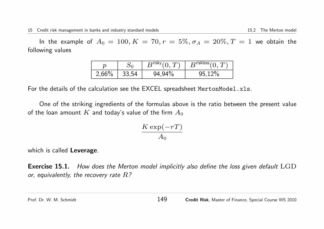
15 Credit risk management in banks and industry standard models 15.2 The Merton model
In the example of A0 = 100, K = 70, r = 5%, σA = 20%, T = 1 we obtain the
following values
p S0 Brisky(0, T ) Briskless(0, T )
2,66% 33,54 94,94% 95,12%
For the details of the calculation see the EXCEL spreadsheet MertonModel.xls.
One of the striking ingredients of the formulas above is the ratio between the present value
of the loan amount K and today’s value of the firm A0
K exp(−rT )
A0
which is called Leverage.
Exercise 15.1. How does the Merton model implicitly also define the loss given default LGD
or, equivalently, the recovery rate R?
Prof. Dr. W. M. Schmidt 149 Credit Risk, Master of Finance, Special Course WS 2010

15 Credit risk management in banks and industry standard models 15.2 The Merton model
Computer Exercise 15.2. For the example above and for different levels of K determine in
EXCEL the implied yield spread s(T ) of the risky bonds relative to a risk free bond. For varying
T plot the corresponding spread curves.
Critical input to the model is today’s value of the firm A0 and its volatility σA which
are both hard to observe directly. In case the firm is also financed by publicly traded equity
one can use equity information such as the stock price S0 and its volatility σS to back out
the corresponding quantities for the firm value process. The Ito-formula yields the following
(approximative) relationship between asset and equity volatility
σSS0 ≈ σAA0N(d1). (25)
Together with the already mentioned formula
S0 = A0N(d1)−K exp(−rT )N(d2), (26)
we have two equations involving the known quantities S0, σS that can be solved for the unknowns
A0, σA.
Prof. Dr. W. M. Schmidt 150 Credit Risk, Master of Finance, Special Course WS 2010

15 Credit risk management in banks and industry standard models 15.3 The KMV model
Computer Exercise* 15.3. Develop an EXCEL spreadsheet to calculate the firm value A0 and
its volatility σA from a given equity price S0 and equity volatility σS! Use the EXCEL solver.
15.3 The KMV model
The San Francisco based company KMV (Kealhofer, McQuown, Vasicek), which is now part of
Moody’s, is one of the world’s leading providers of quantitative credit analysis tools to lenders,
investors, and banks. The model developed by KMV was one of the first portfolio credit risk
models and it is based on the Merton idea. The model by KMV delivers for example default
probabilities and correlations out of observable quantities like leverage, equity price, volatility and
macro economic factors (see [Crosbie and Bohn, 2002]). However, in this section we restrict
ourselves to the problem of default dependence which is critical for all portfolio investigations.
Prof. Dr. W. M. Schmidt 151 Credit Risk, Master of Finance, Special Course WS 2010

15 Credit risk management in banks and industry standard models 15.3 The KMV model
15.3.1 Dependent defaults in the Merton model
We start by reformulating the Merton model (24). Consider the asset returns
ln(AT/A0) = σAWT + rT − σ2AT/2 ∼ N(rT − σ2
AT/2, σ2AT )
= σA√T Y + (r − σ2
A/2)T,
where the random variable Y is the standardized asset return, i.e., it possesses a standard
normal distribution, Y ∼ N(0, 1). The default event D can then be written as
D = {AT < K} ={Y <
ln(K/A0)− rT + σ2AT/2
σA√T
}= {Y < c}
with c = −d2 as the default boundary for the standardized asset return Y and with a default
probability of p = P(D) = N(c). Given the default probability p, for example as a result of a
rating analysis or logit analysis, the corresponding default boundary c is
c = N(−1)
(p). (27)
Prof. Dr. W. M. Schmidt 152 Credit Risk, Master of Finance, Special Course WS 2010

15 Credit risk management in banks and industry standard models 15.3 The KMV model
For two dependent firms (customers, counter parties) with asset values A1T , A
2T we set up a
Merton model for each of them,
Di = {Yi < ci}, i = 1, 2,
with default boundaries c1, c2. To model the dependencies between the defaults we assume now
that Y1, Y2 are correlated variables. Their correlation
ρA
= Corr(Y1, Y2) = Corr(ln(A1T ), ln(A
2T ))
is the so-called asset correlation. The probability of a joint default until time T is then
P(D1 ∩D2) = P(Y1 < c1, Y2 < c2) = N2(c1, c2, ρA),
with N2 denoting the cumulative distribution function of the 2-dimensional standard normal
distribution.
If we model dependent defaults based upon the idea of two correlated Merton models, the
Prof. Dr. W. M. Schmidt 153 Credit Risk, Master of Finance, Special Course WS 2010

15 Credit risk management in banks and industry standard models 15.3 The KMV model
problem reduces to the specification of the asset correlations in practice. One could try to
estimate the asset correlation from a time series of historical stock prices10 if available.
However, KMV and most other applications of the Merton approach model correlations by a
factor model for the asset returns Yi:
Yi =N∑j=1
ωijXj + γiEi. (28)
The variables X1, . . . , XN , Ei are independent standard normal distributed. The quantities
Xj, j = 1, . . . , N describe systematic factors influencing the asset return, such as region,
industry, economic environment etc. Finally the variable Ei is the firm-specific residual factor.
The weight ωij measures the impact of the systematic factor Xj on the value of firm i. Since
Yi should be standard normal distributed we have γ2i = 1−
∑Nj=1 ω
2ij.
The asset correlation of two firms is then determined from the weights of the returns Y1, Y2
10Either using the stock price as proxy for the asset value or backing out the implied asset value considering the stock as call option onthe value of the firm.
Prof. Dr. W. M. Schmidt 154 Credit Risk, Master of Finance, Special Course WS 2010
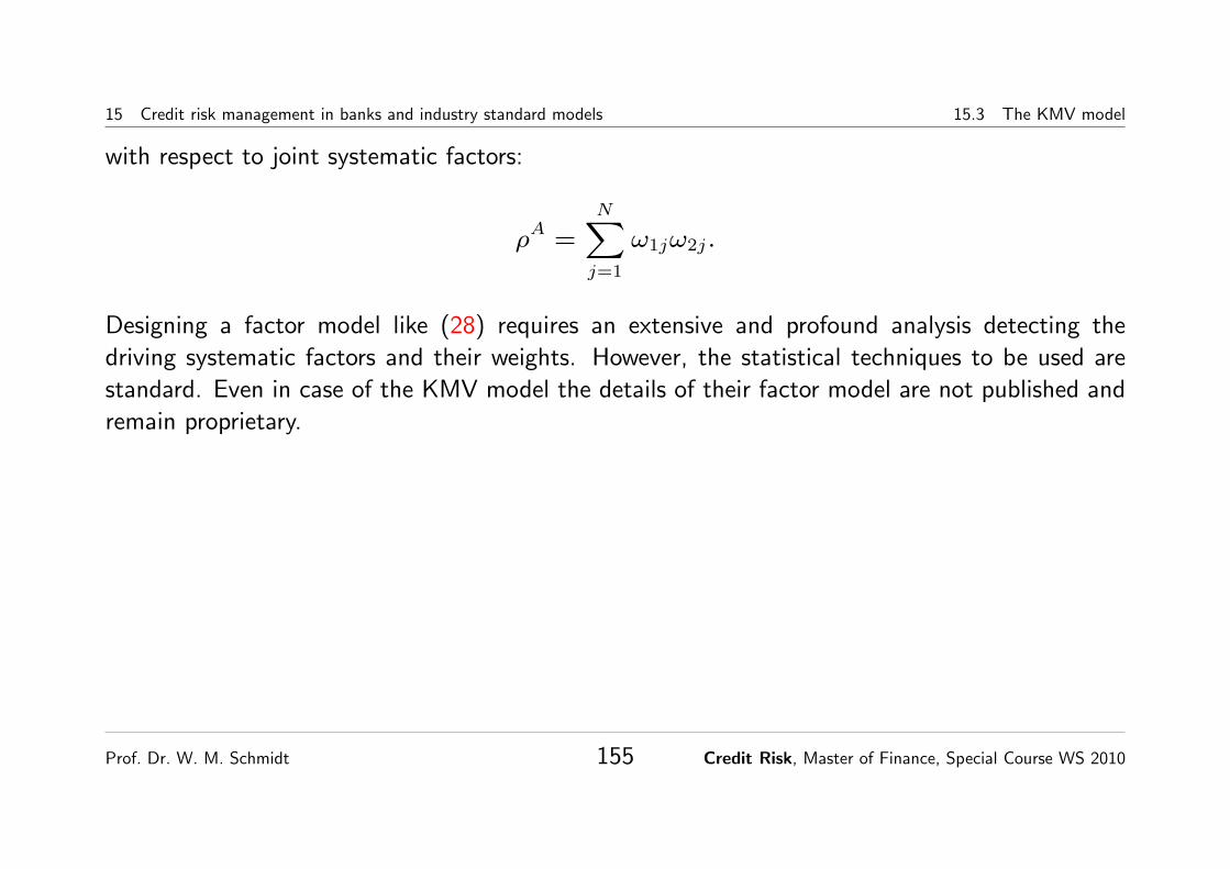
15 Credit risk management in banks and industry standard models 15.3 The KMV model
with respect to joint systematic factors:
ρA
=
N∑j=1
ω1jω2j.
Designing a factor model like (28) requires an extensive and profound analysis detecting the
driving systematic factors and their weights. However, the statistical techniques to be used are
standard. Even in case of the KMV model the details of their factor model are not published and
remain proprietary.
Prof. Dr. W. M. Schmidt 155 Credit Risk, Master of Finance, Special Course WS 2010

15 Credit risk management in banks and industry standard models 15.3 The KMV model
15.3.2 1-Factor dependence and the Basel II formula
Consider a portfolio of n loans with default probabilities pi = P(Di), i = 1, . . . , n and one
and the same asset correlation ρ between any two asset returns Yi, Yj. In terms of the factor
models this yields
Yi =√ρX +
√1− ρEi, i = 1, . . . , n,
with a single joint systematic economic factor X. For credit i the conditional probability of
default pi(x) given that the systematic factors takes the value X = x is then
pi(x) = P(Di|X = x) = P(Yi < N(−1)
(pi)|X = x)
= P(√ρx+
√1− ρEi < N
(−1)(pi))
= P
(Ei <
N(−1)(pi)−√ρx
√1− ρ
)
= N
(N(−1)(pi)−
√ρx
√1− ρ
). (29)
Prof. Dr. W. M. Schmidt 156 Credit Risk, Master of Finance, Special Course WS 2010
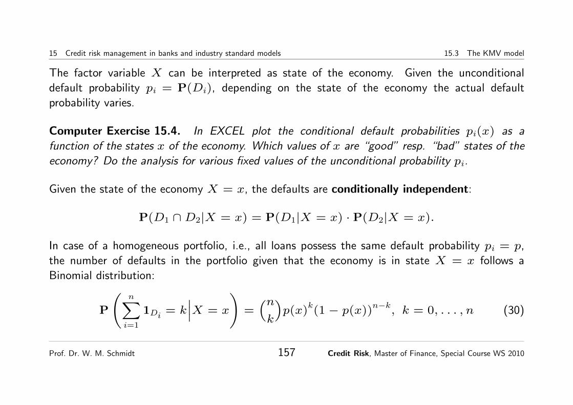
15 Credit risk management in banks and industry standard models 15.3 The KMV model
The factor variable X can be interpreted as state of the economy. Given the unconditional
default probability pi = P(Di), depending on the state of the economy the actual default
probability varies.
Computer Exercise 15.4. In EXCEL plot the conditional default probabilities pi(x) as a
function of the states x of the economy. Which values of x are “good” resp. “bad” states of the
economy? Do the analysis for various fixed values of the unconditional probability pi.
Given the state of the economy X = x, the defaults are conditionally independent:
P(D1 ∩D2|X = x) = P(D1|X = x) · P(D2|X = x).
In case of a homogeneous portfolio, i.e., all loans possess the same default probability pi = p,
the number of defaults in the portfolio given that the economy is in state X = x follows a
Binomial distribution:
P
(n∑i=1
1Di = k∣∣∣X = x
)=(nk
)p(x)
k(1− p(x))
n−k, k = 0, . . . , n (30)
Prof. Dr. W. M. Schmidt 157 Credit Risk, Master of Finance, Special Course WS 2010

15 Credit risk management in banks and industry standard models 15.3 The KMV model
with
p(x) = N
(N(−1)(p)−√ρx√
1− ρ
).
The unconditional distribution of the number of defaults is obtained by integrating over the state
x of the economy,
P
(n∑i=1
1Di = k
)=(nk
)∫ ∞−∞
p(x)k(1−p(x))
n−k 1√
2πexp(−x2
/2)dx, k = 0, . . . , n.
Usually this has to be calculated numerically on a computer.
Here is an example of the loss distribution11 for n = 20 loans, a default probability of
p = 0.5% and an asset correlation of ρA = 50%. The probability of no default in the whole
portfolio is 94.07%.
11Probabilities in logarithmic scale.
Prof. Dr. W. M. Schmidt 158 Credit Risk, Master of Finance, Special Course WS 2010

15 Credit risk management in banks and industry standard models 15.3 The KMV model
Loss distribution KMV Model, 1 Factor
0,00001%
0,00010%
0,00100%
0,01000%
0,10000%
1,00000%
10,00000%
1 2 3 4 5 6 7 8 9 10 11 12 13 14 15 16 17 18 19 20
Number of Defaults
Prof. Dr. W. M. Schmidt 159 Credit Risk, Master of Finance, Special Course WS 2010

15 Credit risk management in banks and industry standard models 15.3 The KMV model
For details of the calculation see the EXCEL spreadsheet KMV1Factor.xls.
Computer Exercise 15.5. In the above example assume that each loan is of nominal amount
100. Calculate the economic capital, CVaR, for this example and a confidence of α = 99%!
Assume a recovery rate of R = 20% for each loan.
We are now in the position to understand the rationale behind the Basel II formula (22). The expected lossE(L|X = x) of the portfolio given a state X = x of the economy is given by
E(L|X = x) = E
(n∑i=1
EADi · LGDi · 1Di∣∣∣X = x
)=
n∑i=1
EADi · LGDi · pi(x).
Now imagine an “infinitely large” portfolio (n → ∞) with “infinitely small” loans (EADi → 0) possessing a 1factor dependence structure. Such a portfolio is called an infinitely fine-grained portfolio.
Prof. Dr. W. M. Schmidt 160 Credit Risk, Master of Finance, Special Course WS 2010

15 Credit risk management in banks and industry standard models 15.3 The KMV model
According to the law of large numbers the sum of independent small variables converges with probability 1 toits expected value12, therefore
P
(L = E(L|X = x) =
∑i
EADi · LGDi · pi(x)∣∣∣X = x
)= 1.
To calculate the economic capital for the portfolio we need the quantile Qα of the distribution of the loss L. Qα isby definition the biggest value such that P(L ≤ Qα) ≤ α. In our situation
α ≥ P(L ≤ Qα)
=
∫ ∞−∞
P(L ≤ Qα|X = x)1√
2πexp(−x2
/2)dx
=
∫ ∞−∞
1{∑i EADi·LGDi·pi(x)≤Qα}1√
2πexp(−x2
/2)dx.
The quantity∑iEADi · LGDi · pi(x) is strictly decreasing13 in x and we can easily solve for the value of the
quantile Qα. Indeed, the set of values x with x ≥ N(−1)(1 − α) has a probability of α and exactly for those
12For more detailed mathematical arguments see, e.g. [Blum et al., 2003], Section 2.5.1.13Of course, assuming EADi > 0.
Prof. Dr. W. M. Schmidt 161 Credit Risk, Master of Finance, Special Course WS 2010

15 Credit risk management in banks and industry standard models 15.3 The KMV model
values x it holds that∑i
EADi · LGDi · pi(x) ≤∑i
EADi · LGDi · pi(N(−1)
(1− α)).
Consequently,
Qα =∑i
EADi · LGDi · pi(N(−1)
(1− α)).
This quantity is, up to the adjustment for the expectation of L, just the economic capital of the portfolio. Thesummand
EADi · LGDi · pi(N(−1)
(1− α))
can be interpreted as risk contribution due to the ith sub-position.
For α = 99.9% taking into account that N(−1)(1 − 0.999) = −N(−1)(0.999) and replacing this informula (29) we end up with
EADi · LGDi · pi(N(−1)
(1− α)) = EADi · LGDi · N(
N(−1)(pi) +√ρN(−1)(0.999)
√1− ρ
),
which is exactly the corresponding expression in the Basel II formula (22).
Prof. Dr. W. M. Schmidt 162 Credit Risk, Master of Finance, Special Course WS 2010

15 Credit risk management in banks and industry standard models 15.4 CreditMetrics
15.4 CreditMetrics
A kind of industry standard was set by RiskMetrics publishing their credit risk methodology
CreditMetrics [G.M.Gupton et al., 1997]. In their framework dependencies are again taken into
account by applying ideas originating from the Merton model and being quite similar to the KMV
approach.
However, we start our discussion of the CreditMetrics model by first looking at the risk of a
single borrower. Contrary to the approaches we have seen so far, CreditMetrics does not consider
exclusively losses from defaults but also losses from changes in credit quality!
As an example consider a loan with face value of 100, time to maturity T and yearly interest
C. We are interested in the risk of this loan, i.e., in the uncertain possible changes in value
∆V = ∆V ∆t over the risk horizon ∆t, in our case for simplicity ∆t = 1 year.
Prof. Dr. W. M. Schmidt 163 Credit Risk, Master of Finance, Special Course WS 2010

15 Credit risk management in banks and industry standard models 15.4 CreditMetrics
Denote r the annually compounded 1-year forward interest rate14. Given a spread s of the
loan relative to the risk free term structure the 1-year forward price of the loan as of today is
Vfwd
0 = C +
T∑t=2
C
(1 + r + s)t−1+
100
(1 + r + s)T−1. (31)
The underlying loan has some credit quality as of today which is measured, for example, by a
rating, lets say BBB. The credit quality (rating) is reflected in today’s spread s of the loan.
However, the credit quality (rating, spread) in 1 year is uncertain. Out of historical data rating
agencies and banks (for their internal rating systems) estimate rating transition probabilities.
14For simplicity of notation we assume a flat forward interest curve.
Prof. Dr. W. M. Schmidt 164 Credit Risk, Master of Finance, Special Course WS 2010

15 Credit risk management in banks and industry standard models 15.4 CreditMetrics
20 Chapter 1. Introduction to CreditMetrics
CreditMetrics™—Technical Document
1.6 Data issues
Given a choice of which rating system (that is, what groupings of similar credits) will be used, CreditMetrics requires three types of data:
• likelihoods of credit quality migration, including default likelihoods;
• likelihoods of joint credit quality migration; and
• valuation estimates (e.g. bonds revalued at forward spreads) at the risk horizon given a credit quality migration.
Together, these data types result in the portfolio value distribution, which determines the absolute amount at risk due to credit quality changes.
1.6.1 Data required for credit migration likelihoods
We showed these individual likelihoods for BBB and single-A rating separately in Tables 1.1 and 1.6 respectively, but this information is more compactly represented in matrix form as shown below in Table 1.8. We call this table a transition matrix. The rat-ings in the first column are the starting or current ratings. The ratings in the first row are the ratings at the risk horizon. For example, the likelihoods in Table 1.8 corresponding to an initial rating of BBB are represented by the BBB row in the matrix. Further, note that each row of the matrix sums to 100%.
Table 1.8One-year transition matrix (%)
Source: Standard & Poor’s CreditWeek (15 April 96)
Transition matrices can be calculated by observing the historical pattern of rating change and default. They have been published by S&P and Moody’s rating agencies, and can be computed based on KMV’s studies, but any provider’s matrix is welcome and usable within CreditMetrics.8 The transition matrix should, however, be estimated for the same time interval as the risk horizon over which we are interested in estimating risks. For instance, a semi-annual risk horizon would use a semi-annual rather than one-year transi-tion matrix.
8 As we discuss later in Chapter 6, adjustments due to limited historical data may sometimes be desirable.
Initial rating
Rating at year-end (%)
AAA AA A BBB BB B CCC Default
AAA 90.81 8.33 0.68 0.06 0.12 0 0 0
AA 0.70 90.65 7.79 0.64 0.06 0.14 0.02 0
A 0.09 2.27 91.05 5.52 0.74 0.26 0.01 0.06
BBB 0.02 0.33 5.95 86.93 5.30 1.17 0.12 0.18
BB 0.03 0.14 0.67 7.73 80.53 8.84 1.00 1.06
B 0 0.11 0.24 0.43 6.48 83.46 4.07 5.20
CCC 0.22 0 0.22 1.30 2.38 11.24 64.86 19.79
Prof. Dr. W. M. Schmidt 165 Credit Risk, Master of Finance, Special Course WS 2010

15 Credit risk management in banks and industry standard models 15.4 CreditMetrics
For each possible future rating we assign a corresponding (forward) credit spread relative to
the risk free interest rate, for example,
Rating after 1 year Forward spread s
AAA 0,00%
AA 0,10%
A 0,20%
BBB 0,50%
BB 1,90%
B 3,20%
CCC 10,00%
These spreads are usually taken from historical experience, i.e., they quantify the average spread
in the respective rating category.
For each possible future rating of the borrower one can now determine from formula (31) the
potential value of the loan after 1 year.
Prof. Dr. W. M. Schmidt 166 Credit Risk, Master of Finance, Special Course WS 2010

15 Credit risk management in banks and industry standard models 15.4 CreditMetrics
As Example consider a loan with face value of 100, C = 5 and T = 10 years to maturity.
Assume r = 4% for the risk free interest rate. We obtain the following values depending on the
rating in 1 year
AAA AA A BBB BB B CCC D (default)
112,44 111,66 110,89 108,63 98,85 90,79 60,48 45,00
For example, in case of a rating of A,
110, 89 = 5 +
10∑t=2
5
(1 + 0, 04 + 0, 002)t−1+
100
(1 + 0, 04 + 0, 002)9.
In the default state, i.e. “rating” D, we assumed a recovery rate of R = 45%.
Combining this with the rating transition probabilities we end up with a probability distributionon the possible future values and thus the possible value changes ∆V . In the example, assumingfor the loan a current rating of BBB,
Prof. Dr. W. M. Schmidt 167 Credit Risk, Master of Finance, Special Course WS 2010

15 Credit risk management in banks and industry standard models 15.4 CreditMetrics
Rating in 1 year probability value ∆V
AAA 0,02% 112,44 3,80AA 0,33% 111,66 3,03A 5,95% 110,89 2,26
BBB 86,93% 108,63 0,00BB 5,30% 98,85 -9,78B 1,17% 90,79 -17,85
CCC 0,12% 60,48 -48,15D 0,18% 45,00 -63,63
Probability distribution of value change
0,01%
0,10%
1,00%
10,00%
100,00%
3,803,032,260,00-9,78-17,85-48,15-58,63∆V
Prob
abilit
y
Prof. Dr. W. M. Schmidt 168 Credit Risk, Master of Finance, Special Course WS 2010

15 Credit risk management in banks and industry standard models 15.4 CreditMetrics
See the EXCEL spreadsheet CreditMetrics1Loan.xls for all details of the calculation.
Now we are in the position to calculate the economic capital for a position consisting of one
single loan in the framework of the CreditMetrics model.
Exercise 15.6. Determine the economic capital for the loan from the example assuming a
confidence of α = 95%.
The model can be refined in many directions. For example, one can use an arbitrarily fine
grained rating structure and, for each rating, one can consider a complete term structure of
spreads (spread curve).
What is still unanswered for the CreditMetrics model is how the important issue of
dependencies between defaults is resolved. For that problem CreditMetrics uses somewhat
refined ideas from the Merton model. There, default is triggered by the standardized asset return
Y falling below a certain threshold cD. Now starting from today’s rating, lets say BBB, we
introduce further thresholds cAA > cA > · · · > cD for Y with the interpretation that
Prof. Dr. W. M. Schmidt 169 Credit Risk, Master of Finance, Special Course WS 2010
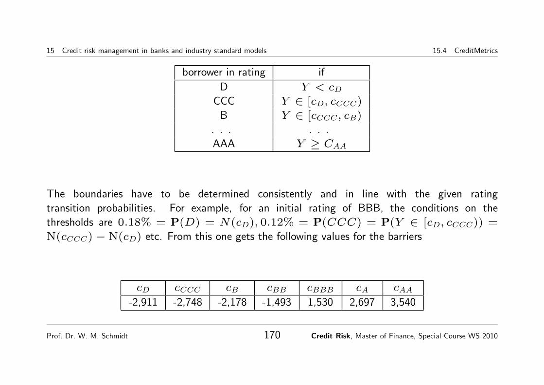
15 Credit risk management in banks and industry standard models 15.4 CreditMetrics
borrower in rating if
D Y < cDCCC Y ∈ [cD, cCCC)
B Y ∈ [cCCC, cB)
. . . . . .
AAA Y ≥ CAA
The boundaries have to be determined consistently and in line with the given rating
transition probabilities. For example, for an initial rating of BBB, the conditions on the
thresholds are 0.18% = P(D) = N(cD), 0.12% = P(CCC) = P(Y ∈ [cD, cCCC)) =
N(cCCC)− N(cD) etc. From this one gets the following values for the barriers
cD cCCC cB cBB cBBB cA cAA-2,911 -2,748 -2,178 -1,493 1,530 2,697 3,540
Prof. Dr. W. M. Schmidt 170 Credit Risk, Master of Finance, Special Course WS 2010
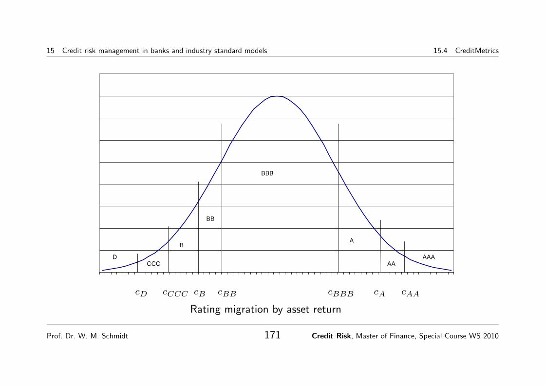
15 Credit risk management in banks and industry standard models 15.4 CreditMetrics
Rating migration by asset return
cD cCCC cB cBB cBBB cA cAA
Rating-Migration durch Assetreturn
BBB
BB
B
CCCD
A
AAAAA
Prof. Dr. W. M. Schmidt 171 Credit Risk, Master of Finance, Special Course WS 2010

15 Credit risk management in banks and industry standard models 15.4 CreditMetrics
Now for each loan i in the portfolio, default and changes in credit quality are modeled by a
corresponding asset return Yi. Dependencies are generated by considering the asset returns of
the different borrowers to be correlated with some asset correlation.
For a portfolio with i = 1, . . . , n loans the distribution of its future uncertain changes in
value ∆V can be determined usually only by performing a Monte Carlo simulation. To that end
the following steps have to be carried out:
• For each loan i possible future values are calculated for all possible future ratings applying
respective spreads and assuming a certain recovery rate.
• For each position i starting from its current rating one has to determine the thresholds
ciD, ciCCC, . . . , c
iAA according to the given rating transition probabilities.
• The standard normal distributed asset returns Yi, i = 1, . . . , n, with correlation matrix
ρij = Corr(Yi, Yj) are simulated N times.
• For each simulation, depending on the value of Yi the future rating is determined which gives
us the future value of that loan i in the given simulation scenario. The values are added up
to a portfolio value for the simulation path.
Prof. Dr. W. M. Schmidt 172 Credit Risk, Master of Finance, Special Course WS 2010

15 Credit risk management in banks and industry standard models 15.4 CreditMetrics
• The result are N simulated future portfolio values and one can estimate from that any desired
risk measure, e.g., the economic capital, empirically.
Computer Exercise 15.7. Using the EXCEL Sheets CreditMetrics.xls calculate the eco-
nomic capital (α = 99%) for a portfolio consisting of two loans with
face value interest time to maturity rating recovery rate
100 4% 10 BBB 30%
100 6% 7 A 40%
The riskless interest rate is assumed to be r = 4%. Transition probabilities and spreads per
rating are already specified in the sheet. Use an asset correlation of ρA = 50%.
Prof. Dr. W. M. Schmidt 173 Credit Risk, Master of Finance, Special Course WS 2010

15 Credit risk management in banks and industry standard models 15.5 Credit Risk+
15.5 Credit Risk+
The CreditRisk+ model proposed by Credit Suisse First Boston
[Credit Suisse First Boston, 1997], is another popular industry standard approach to portfo-
lio credit risk. The model is based on the observation that default probabilities face fluctuations
and should therefore considered as being random themselves.
CREDITRISK + 13
2Modelling Credit Risk
Credit Risk Measurement
Exposures Default Rates
CREDITRISK+ Model
RecoveryRates
Default RateVolatilities
Credit Risk Measurement
Exposures Default Rates
CREDITRISK+ Model
RecoveryRates
Default RateVolatilities
Table 3:
Default rate standard
deviations (%)
Figure 5:
Defaulted bank loan
price distribution
Fre
qu
en
cy
2.6.4 Default Rate Volatilities
Published default statistics include average default rates over many years. As shown previously, actual
observed default rates vary from these averages. The amount of variation in default rates about these averages
can be described by the volatility (standard deviation) of default rates. As can be seen in the following table,
the standard deviation of default rates can be significant compared to actual default rates, reflecting the high
fluctuations observed during economic cycles.
One-year default rate (%)
Credit rating Average Standard deviation
Aaa 0.00 0.0
Aa 0.03 0.1
A 0.01 0.0
Baa 0.12 0.3
Ba 1.36 1.3
B 7.27 5.1
Source: Carty & Lieberman, 1996, Moody’s Investors Service Global Credit Research
The default rate standard deviations in the above table were calculated over the period from 1970 to 1996
and therefore include the effect of economic cycles.
2.6.5 Recovery Rates
In the event of a default of an obligor, a firm generally incurs a loss equal to the amount owed by the obligor
less a recovery amount, which the firm recovers as a result of foreclosure, liquidation or restructuring of the
defaulted obligor or the sale of the claim. Recovery rates should take account of the seniority of the obligation
and any collateral or security held.
Recovery rates are subject to significant variation. For example, the figure below shows the price distribution
of defaulted bank loans and illustrates that there is a large degree of dispersion.
Source: Defaulted Bank Loan Recoveries (November 1996) , Moody’s Investors Service Global Credit Research
$0
-$1
0
$1
1-$
20
$2
1-$
30
$3
1-$
40
$4
1-$
50
$5
1-$
60
$6
1-$
70
$7
1-$
80
$8
1-$
90
$9
1-$
10
0
14
12
10
8
6
4
2
0
Prof. Dr. W. M. Schmidt 174 Credit Risk, Master of Finance, Special Course WS 2010

15 Credit risk management in banks and industry standard models 15.5 Credit Risk+
From now on we denote by
p = P(D)
the expected, average default probability. In the framework of the CreditRisk+ model the
”default probability” is a random variable P taking, of course, values in the interval [0, 1], and
with expectation E(P ) = p. In the model the default event is the result of a two step process
• generate (”roll dice”) a value p of the random variable P
• generate the default event by ”tossing a coin” with probability p of ”success”=default
On the computer this two step process can be realized as follows. For U a uniformly distributed
random variable on [0, 1] which is independent of P the default event D can be modeled as
D = {U < P}.
Prof. Dr. W. M. Schmidt 175 Credit Risk, Master of Finance, Special Course WS 2010

15 Credit risk management in banks and industry standard models 15.5 Credit Risk+
In fact, we have as desired
P(D|P = p) = P(U < p} = p
P(D) =
∫P(D|P = p)fP (p)dp
=
∫p fP (p) dp
= E(P ) = p,
where fP stands for the probability distribution density of the random variable P .
For two credits with default events D1, D2 , given realized values for P1, P2, the default events
are assumed to be independent, i.e.,
P(D1 ∩D2|P1 = p1, P2 = p2) = p1 · p2.
Prof. Dr. W. M. Schmidt 176 Credit Risk, Master of Finance, Special Course WS 2010

15 Credit risk management in banks and industry standard models 15.5 Credit Risk+
A simple approach to model the random default probability P consists in setting P = p(X)
with some driving random variable X and some function p(x). Examples are
p(X) = exp(−c ·X) (32)
p(X) = exp(−(c+X)) (33)
with an arbitrary non-negative random variable X and constant c > 0 to be calibrated to match
the given expectation E(P ) = p.
For two loans i = 1, 2 with default event Di and average default probability P(Di) = pithe model assumes that each of the random default probabilities Pi is driven by a certain function
pi(x) of a factor variable Xi,
Pi = pi(Xi).
As we shall see, dependencies are generated by the fact, that the variables Xi are dependent;
then, the probabilities Pi are dependent as well. In the extreme case X1 = X2 = X, the
random default probability for both loans is determined by a joint ”sector variable” X. Let us
Prof. Dr. W. M. Schmidt 177 Credit Risk, Master of Finance, Special Course WS 2010

15 Credit risk management in banks and industry standard models 15.5 Credit Risk+
investigate how this impacts the probability of a joint default, and, by that, the event correlation
ρE. With fX denoting the density of X we obtain
P(D1 ∩D2) =
∫P(D1 ∩D2|X = x)fX(x)dx
=
∫P(D1 ∩D2
∣∣∣P1 = p1(x), P2 = p2(x))fX(x)dx
=
∫p1(x)p2(x)fX(x)dx
= p1p2 + COV(p1(X), p2(X)),
and from that and the definition (20) of the event correlation,
ρE
=COV(p1(X), p2(X))√p1(1− p1)p2(1− p2)
. (34)
Intuitively, the higher the variability (variance) of X the higher the above covariance and thus
the default correlation.
Prof. Dr. W. M. Schmidt 178 Credit Risk, Master of Finance, Special Course WS 2010

15 Credit risk management in banks and industry standard models 15.5 Credit Risk+
Richer but still tractable correlation structures can be generated by a sector model of the
form
Pi = pi
(∑s
ωisXs
)with independent sector variables Xs and weights ωis.
CreditRisk+ proposes a Gamma distribution for the sector variable X. The Gamma
distribution admits two parameters α, β and its density is given by15
fX(x) =1
βαΓ(α)exp
(−x
β
)xα−1
, x > 0
E(X) = αβ
V(X) = αβ2.
15The Gamma function is defined as Γ(α) =∫∞0 xα−1e−xdx, α > 0.
Prof. Dr. W. M. Schmidt 179 Credit Risk, Master of Finance, Special Course WS 2010

15 Credit risk management in banks and industry standard models 15.5 Credit Risk+
The expectation E exp(−cX) is straightforward to calculate,
E exp(−cX) =1
(1 + cβ)α. (35)
In case of a model setup as in (32) the calibration of the constant c becomes straightforward,
c =(p)−1/α − 1
β.
Let us now investigate how the loss distribution for a whole portfolio comes out of
the CreditRisk+ approach. To simplify the exposition consider a homogeneous portfolio of
i = 1, . . . , n loans, each with one and the same notional amount N and the same recovery rate
R. The loss Li for loan i is clearly
Li = 1DiN(1− R).
Prof. Dr. W. M. Schmidt 180 Credit Risk, Master of Finance, Special Course WS 2010

15 Credit risk management in banks and industry standard models 15.5 Credit Risk+
The overall loss L =∑n
i=1Li of a homogenous portfolio is completely determined by the
number of defaults ξ
ξ =
n∑i=1
1Di,
L = ξ N (1− R).
The random variable ξ takes values in the range {0, 1, . . . , n}.
To simplify the exposition we further assume that the default probability takes one and the
same value p for each loan in the portfolio and that the random default probabilities Pi are
dependent via a single joint sector variable X,
Pi = p(X), i = 1, . . . , n, p = E(p(X)).
For each concrete value x of the random variable X the conditional distribution of the number ξ
of defaults is a Binomial distribution (compare also (30))
ξ|X = x ∼ B (n, p(x)) . (36)
Prof. Dr. W. M. Schmidt 181 Credit Risk, Master of Finance, Special Course WS 2010

15 Credit risk management in banks and industry standard models 15.5 Credit Risk+
The crux of the CreditRisk+ model is, among others, the fact that also the unconditional
distribution of the number of defaults and thus distribution of the loss L can be expressed in
closed form. If the sector variable X is assumed to be Gamma distributed and we follow the
setup (32), i.e., p(x) = exp(−cx), then
P(L = k ·N(1− R)) = P(ξ = k)
=
∫ ∞0
P(ξ = k|X = x)fX(x)dx
= . . .
=
n−k∑i=0
(n− ki
)(nk
)(−1)
i 1
(1 + c(k + i)β)α.
Example: Consider a portfolio of n = 20 homogeneous loans with average default probability
p = 1, 0%. For an event correlation of ρE = 5% resp. ρE = 15% we obtain the following loss
distribution16:16The probability of no default in the portfolio is, dependent on the correlation, 87% resp. 91%. Probabilities are shown in logarithmic
scale.
Prof. Dr. W. M. Schmidt 182 Credit Risk, Master of Finance, Special Course WS 2010

15 Credit risk management in banks and industry standard models 15.5 Credit Risk+
Loss Distribution CR+
0,0000%
0,0000%
0,0000%
0,0000%
0,0001%
0,0010%
0,0100%
0,1000%
1,0000%
10,0000%
100,0000%
0 1 2 3 4 5 6 7 8 9 10 11 12 13 14 15 16 17 18 19 20
Number of defaults
log
(Pro
babi
lity)
5%15%
Prof. Dr. W. M. Schmidt 183 Credit Risk, Master of Finance, Special Course WS 2010

15 Credit risk management in banks and industry standard models 15.6 Comparison KMV/CreditMetrics versus CreditRisk+
See the EXCEL spreadsheet CreditPortfolioModels.xls for details of the calculation.
15.6 Comparison KMV/CreditMetrics versus CreditRisk+
Although the credit portfolio risk models considered so far are conceptually quite different there
are some striking similarities.
First of all, in case that we consider only two rating categories, default and no default, the
CreditMetrics model basically coincides with the KMV model.
Concerning the modeling of dependencies, in the situation of a 1-factor dependence structure
and a homogeneous portfolio, both approaches, KMV/CreditMetrics and CreditRisk+, are in
principle quite similar. Both models generate dependence between defaults in a portfolio by
a joint factor or sector variable X. The conditional default probability p(x) given the state
X = x is given by formulas (29) and (32), respectively. Given the state x of the factor/sector
variable X, defaults are conditionally independent and the number of defaults follows a Binomial
Prof. Dr. W. M. Schmidt 184 Credit Risk, Master of Finance, Special Course WS 2010

15 Credit risk management in banks and industry standard models 15.6 Comparison KMV/CreditMetrics versus CreditRisk+
distribution (cf. (30), (36))
P
(n∑i=1
1Di = k∣∣∣X = x
)=(nk
)p(x)
k(1− p(x))
n−k, k = 0, . . . , n.
The unconditional distribution of the number of defaults is obtained by integrating the conditional
distribution over the states x weighted by the density fX(x) of the factor/sector variable X
P
(n∑i=1
1Di = k
)=(nk
)∫ ∞−∞
p(x)k(1− p(x))
n−kfX(x)dx, k = 0, . . . , n.
KMV/CreditMetrics CreditRisk+
p(x) N
(N(−1)(p)−√ρx√
1−ρ
)exp(−cx)
fX(x) 1√2π
exp(−x2/2) 1βαΓ(α) exp(−x
β)xα−1, x > 0
Prof. Dr. W. M. Schmidt 185 Credit Risk, Master of Finance, Special Course WS 2010

15 Credit risk management in banks and industry standard models 15.6 Comparison KMV/CreditMetrics versus CreditRisk+
For comparison the following picture shows the distribution17 of the number of defaults for both
models in case of a homogeneous portfolio with n = 20, p = 1.0%. All other model parameters
have been calibrated to imply an event correlation of 10%.
17Probabilities in logarithmic scale.
Prof. Dr. W. M. Schmidt 186 Credit Risk, Master of Finance, Special Course WS 2010

15 Credit risk management in banks and industry standard models 15.6 Comparison KMV/CreditMetrics versus CreditRisk+
Loss Distribution KMV vs CreditRisk+
0,0000%
0,0000%
0,0001%
0,0010%
0,0100%
0,1000%
1,0000%
10,0000%
100,0000%
0 1 2 3 4 5 6 7 8 9 10 11 12 13 14 15 16 17 18 19 20
Number of defaults
log
(Pro
babi
lity)
KMVCR+
Prof. Dr. W. M. Schmidt 187 Credit Risk, Master of Finance, Special Course WS 2010
15 Credit risk management in banks and industry standard models 15.6 Comparison KMV/CreditMetrics versus CreditRisk+
References
[Basle Committee on Banking Supervision, 1988] Basle Committee on Banking Supervision
(1988). International convergence of capital measurement and capital standards. Tech-
nical report, Bank for International Settlements. 133
[Basle Committee on Banking Supervision, 2003] Basle Committee on Banking Supervision
(2003). The new basel capital accord, third consultative paper. Technical report, Bank for
International Settlements. 137, 140
[Bielecki and Rutkowski, 2002] Bielecki, T. R. and Rutkowski, M. (2002). CreditRisk: Modeling,
Valuation and Hedging. Springer Verlag, New York. 76, 79
[Blum et al., 2003] Blum, C., Overbeck, L., and Wagner, C. (2003). An Introduction to Credit
Risk Modeling. Chapmann & Hall. 1, 161
[Credit Suisse First Boston, 1997] Credit Suisse First Boston (1997). CreditRisk+ - A Credit
Risk Management Framework. Technical report, Credit Suisse First Boston. 174
[Crosbie and Bohn, 2002] Crosbie, P. J. and Bohn, J. R. (2002). Modeling Default Risk.
Technical report, KMV Corporation. 151
Prof. Dr. W. M. Schmidt 188 Credit Risk, Master of Finance, Special Course WS 2010

15 Credit risk management in banks and industry standard models 15.6 Comparison KMV/CreditMetrics versus CreditRisk+
[Duffie and Singleton, 2003] Duffie, D. and Singleton, K. J. (2003). Credit Risk. Princeton
University Press. 1, 76, 79
[Duffie and Zhu, 2009] Duffie, D. and Zhu, H. (2009). Does a central clearing counterparty
reduce counterparty risk? Working paper, Stanford University. 61
[Embrechts et al., 1999] Embrechts, P., McNeil, A., and Straumann, D. (1999). Correlation:
pitfalls and alternatives. Risk, 12(5):93–113. 106
[Frey et al., 2001] Frey, R., McNeil, A., and M., N. (2001). Copulas and credit models. Risk,
pages 111–113. 106
[G.M.Gupton et al., 1997] G.M.Gupton, C.C.Finger, and M.Bhatia (1997). CreditMetrics -
Technical Document. Technical report, Morgan Guaranty Trust Co. 120, 163
[Hull and White, 2001] Hull, J. and White, A. (2001). Valuing Credit Default Swaps II: Modeling
Default Correlations. The Journal of Derivatives, pages 12–21. 75, 100
[International Swap and Derivatives Association, 2003] International Swap and Derivatives Asso-
ciation (2003). Credit Derivatives Documentation. 114
[Jorion, 2009] Jorion, P. (2009). Financial risk manager handbook. John Wiley & Sons Inc, 5th
edition. 1
Prof. Dr. W. M. Schmidt 189 Credit Risk, Master of Finance, Special Course WS 2010

15 Credit risk management in banks and industry standard models 15.6 Comparison KMV/CreditMetrics versus CreditRisk+
[Lando, 2004] Lando, D. (2004). Credit Risk Modeling. Princeton University Press. 1, 76, 79
[Li, 2000] Li, D. X. (2000). On default correlation: a copula function approach. Journal of Fixed
Income, 9:43–45. 106
[Longstaff and Schwartz, 1995] Longstaff, F. A. and Schwartz, E. S. (1995). A simple approach
to valuing risky fixed and floating rate debt. Journal of Finance, 50(3):789–819. 74
[Mason, 2009] Mason, D. M. (2009). Credit Derivatives: Market Solutions to the Market Crisis.
Technical Report 2262, Backgrounder, The Heritage Foundation. 58
[Merton, 1974] Merton, R. (1974). On the pricing of corporate debt: The risk structure of
interest rates. Journal of Finance, 29:449–470. 74, 146
[Nelsen, 1999] Nelsen, R. (1999). An introduction to copulas. Springer Verlag, New York. 106
[Poor’s, 2002] Poor’s, S. . (2002). Rating performance 2001. Technical report, Standard &
Poor’s. 121, 122
[Saunders and Allen, 2002] Saunders, A. and Allen, L. (2002). Credit risk measurement. Wiley.
1
[Schmidt and Ward, 2002] Schmidt, W. and Ward, I. (2002). Pricing default baskets. Risk,
pages 111–114. 106
Prof. Dr. W. M. Schmidt 190 Credit Risk, Master of Finance, Special Course WS 2010

15 Credit risk management in banks and industry standard models 15.6 Comparison KMV/CreditMetrics versus CreditRisk+
[Schonbucher, 2003] Schonbucher, P. J. (2003). Credit Derivatives Pricing Models. Wiley. 79
[Stulz, 2009] Stulz, R. (2009). Credit default swaps and the credit crisis. 56
[Zhou, 1997] Zhou, C. (1997). A jump-diffusion approach to modeling credit risk and valuing
defaultable securities. Technical report, Federal Reserve Board. 75
Prof. Dr. W. M. Schmidt 191 Credit Risk, Master of Finance, Special Course WS 2010


