Credit value adjustment for credit default swaps via the structural
24
The Journal of Credit Risk (123–146) Volume 5/Number 2, Summer 2009 Credit value adjustment for credit default swaps via the structural default model Alexander Lipton Bank of America Merrill Lynch, 2 King Edward Street, London, EC1 1HQ; email: [email protected] Artur Sepp Bank of America Merrill Lynch, 2 King Edward Street, London, EC1 1HQ; email: [email protected] We present a multi-dimensional jump-diffusion version of a structural default model and show how to use it in order to value the credit value adjustment for a credit default swap. We develop novel analytical and numerical methods for solving the corresponding boundary value problem with a special emphasis on the role of negative asset value jumps. Using recent market data, we show that under realistic assumptions credit value adjustment greatly reduces the value of a credit default swap sold by a risky counterparty compared with one sold by a non-risky counterparty. We identify features having the biggest impact on credit value adjustment: namely, default correlation and spread volatility. 1 INTRODUCTION 1.1 Motivation Credit default swaps (CDSs) are fundamental building blocks of more complicated credit instruments such as synthetic collateralized debt obligations (CDOs). Typi- cally their prices are readily available; they are used as inputs for more complicated models. For some time now it has been realized that, in order to value CDSs properly, counterparty effects have to be taken into account. However, conventional tools used for valuing the credit value adjustment (CVA) for over-the-counter (OTC) deriva- tives are not adequate for CDSs due to the pronounced correlation effect. The key goal of this article is to present a novel valuation methodology for the valuation of CVA for CDSs.As a prerequisite for achieving this goal, we build a new multi-name structural default model (SDM). Recall that a typical CDS is an OTC contract between a protection buyer and a protection seller that insures the protection buyer against a possible default of We are grateful to several colleagues at Bank ofAmerica Merrill Lynch for stimulating discussions. The opinions expressed in this paper are those of the authors and do not necessarily reflect the views and policies of Bank of America Merrill Lynch. 123
Transcript of Credit value adjustment for credit default swaps via the structural

The Journal of Credit Risk (123–146) Volume 5/Number 2, Summer 2009
Credit value adjustment for credit defaultswaps via the structural default model
Alexander LiptonBank of America Merrill Lynch, 2 King Edward Street, London, EC1 1HQ;email: [email protected]
Artur SeppBank of America Merrill Lynch, 2 King Edward Street, London, EC1 1HQ;email: [email protected]
We present a multi-dimensional jump-diffusion version of a structural defaultmodel and show how to use it in order to value the credit value adjustment fora credit default swap. We develop novel analytical and numerical methods forsolving the corresponding boundary value problem with a special emphasis onthe role of negative asset value jumps. Using recent market data, we show thatunder realistic assumptions credit value adjustment greatly reduces the value ofa credit default swap sold by a risky counterparty compared with one sold by anon-risky counterparty. We identify features having the biggest impact on creditvalue adjustment: namely, default correlation and spread volatility.
1 INTRODUCTION
1.1 Motivation
Credit default swaps (CDSs) are fundamental building blocks of more complicatedcredit instruments such as synthetic collateralized debt obligations (CDOs). Typi-cally their prices are readily available; they are used as inputs for more complicatedmodels. For some time now it has been realized that, in order to value CDSs properly,counterparty effects have to be taken into account. However, conventional tools usedfor valuing the credit value adjustment (CVA) for over-the-counter (OTC) deriva-tives are not adequate for CDSs due to the pronounced correlation effect. The keygoal of this article is to present a novel valuation methodology for the valuation ofCVA for CDSs. As a prerequisite for achieving this goal, we build a new multi-namestructural default model (SDM).
Recall that a typical CDS is an OTC contract between a protection buyer anda protection seller that insures the protection buyer against a possible default of
We are grateful to several colleagues at Bank ofAmerica Merrill Lynch for stimulating discussions.The opinions expressed in this paper are those of the authors and do not necessarily reflect theviews and policies of Bank of America Merrill Lynch.
123

124 A. Lipton and A. Sepp
the reference name in exchange for periodic payments up to the termination ofthe contract, which occurs when the CDS expires or the reference name defaults,whichever comes first. Cash flows to the protection buyers from protection sellersand vice versa are called default legs and coupon legs (CLs), respectively.
When a protection buyer buys a CDS protection from a risky protection seller,it has to account for two types of exposure. First, there is market risk due to thechanges in the mark-to-market (MtM) value of the corresponding CDS caused bychanges in credit spread and interest rate. Second, there is credit risk due to the factthat the protection seller can default prior to CDS termination. During the life of aCDS contract, a realized loss due to the counterparty exposure can arise when theprotection seller defaults before the reference name, provided that the MtM of theCDS is positive for the protection buyer, since only a fraction of the MtM value ofthe existing CDS contract can be recovered. If the MtM of the CDS is negative tothe protection buyer, this CDS is unwound at market price.
Since the protection buyer realizes positive MtM gains when the credit qualityof the reference name deteriorates (because the probability of receiving protectionpayment increases), the realized loss due to protection seller default is particularlybig if the credit quality of the reference name and the protection seller are positivelycorrelated and deteriorate simultaneously. In order to account for the correlationeffect in a meaningful way, we introduce a novel multi-name SDM based on corre-lated jump-diffusion processes. In this model, a typical default of a single name istriggered by a sudden drop in the asset value followed by its gradual deterioration,which is a pattern observed in practice, in particular, in the case of financial institu-tions. In order to calculate CVA for CDSs, we combine the dynamics for asset valuesfor the reference name and the protection seller and describe it via two correlatedjump-diffusion processes.
We show that CVA (which we define as the maximal expected loss for the protec-tion buyer) can be interpreted as a two-dimensional down-and-in digital option withthe down barrier being triggered when the value of protection seller assets crosses itsdefault barrier and the option rebate being determined by the value of the referencename assets at the time of barrier crossing. Under realistic assumptions, CVA canbe very significant, reducing the present value of the default leg of the correspond-ing CDS by 5–30%. Naturally, the magnitude of this reduction is sensitive to thechoice of both volatility and correlation for the corresponding dynamics. Our resultsindicate that CVA for OTC CDSs should be viewed as a first-order effect.
At inception the spread of a CDS contract is set in such a way that the MtMvalue of the contract is zero, so that the option underlying CVA is at-the-money.Accordingly, its value is highly sensitive to the volatility of the asset values for boththe reference name and the protection seller as well as to their correlation. Thus, inorder to evaluate CVA accurately, we need to model the correlated dynamics of thereference name and the protection seller in a convincing manner.
The Journal of Credit Risk Volume 5/Number 2, Summer 2009

Credit value adjustment for credit default swaps via the structural default model 125
Between 2001 and 2007 the notional value of outstanding CDSs grew by a factorof 100 and the outstanding notional amount of credit derivatives has become huge.Due to the turbulence in the credit markets, the counterparty problem has becomecritical for the financial industry. This has resulted in a dramatic shrinkage of themarket. According to the most recent International Swaps and Derivatives Associ-ation survey published on April 22, 2009 (see www.isda.org), the notional valueof outstanding CDSs decreased to US$39 trillion as of December 31, 2008 fromUS$55 trillion in the middle of the year and US$62 trillion as of December 31,2007. For comparison, the notional value of outstanding interest rate derivativesis about US$382 trillion, while the notional value of equity derivatives is aboutUS$10 trillion. Recently, in order to improve market transparency and liquidity,more than 2,000 banks, hedge funds and asset managers trading CDSs agreed to a“Big Bang Protocol”. Regulators and legislators have repeatedly called for an indus-try overhaul since the swaps were blamed for playing a pivotal role in the collapseof Lehman Brothers and the disintegration of AIG. All this makes the evaluation andhedging of CVA for CDSs vital for the financial system as a whole.
1.2 Prior research
Merton (1974) introduces the original SDM. He assumes that a firm’s asset value isdriven by a lognormal diffusion and the firm defaults at the time of debt maturity ifthe notional of the debt exceeds the asset value. His ideas were extended by severalresearchers, notably by Black and Cox (1976), who propose the idea of the contin-uous default barrier. In the early 2000s, when CDS contracts gained popularity andbecame liquid, it was realized that the classical SDM based on lognormal dynamicscannot explain high short-term CDS spreads traded in the market. This is due tothe fact that in such a model a default event is predictable, so that the probabilityof a non-distressed firm defaulting in the near term is close to zero. To account forthis effect, the SDM has been extended to incorporate curvilinear barriers (see, forexample, Hyer et al (1998); Hull and White (2001)), sudden jumps in a firm’s value(see, for example, Zhou (2001a); Hilberink and Rogers (2002); Lipton (2002); Lip-ton et al (2007); Sepp (2004, 2006)) or default barrier uncertainty (see, for example,Finger et al (2002)).
Two-dimensional extensions of SDM are studied by Zhou (2001b), Hull andWhite(2001), Haworth et al (2006), Blanchet-Scalliet and Patras (2008) and several otherresearchers, who consider bivariate correlated lognormal dynamics for two firmsand derive analytical formulas for their joint survival. Multi-dimensional extensionsof the SDM are described by JPMorgan (1997), Li (2000) and many others, whouse Gaussian copulas to describe correlated default times for a portfolio of names.More recently a version of a multi-dimensional SDM with jumps has been pro-posed by Kiesel and Scherer (2007), who develop a mixture of semi-analytical andMonte Carlo tools for its calibration and usage.
Research Paper www.thejournalofcreditrisk.com
126 A. Lipton and A. Sepp
This article is devoted specifically to counterparty risk. This topic has been investi-gated by numerous researchers, for instance, Jarrow and Turnbull (1995), Jarrow andYu (2001), Leung and Kwok (2005) and Crepey et al (2009) develop the so-calledreduced-form default model and analyze the counterparty risk in its framework; Hulland White (2001) and Blanchet-Scalliet and Patras (2008) model the evolution ofthe reference name and the protection seller by two correlated Brownian motionsand analyze bivariate default effects; Turnbull (2005) derives model-free upper andlower bounds for the counterparty exposure; Pykhtin and Zhu (2006) and Gregory(2009) use the Gaussian copula approach to study defaults of the reference nameand the protection seller; Brigo and Chourdakis (2008) consider correlated dynam-ics of the credit spreads. By necessity, this list is not exhaustive and could easily beextended.
1.3 New findings
We propose a new SDM based on jump-diffusion dynamics for a single name andextend it to the multi-dimensional case. As an asset value driver we use an additiveprocess, which is a jump-diffusion process with time-inhomogeneous increments(see Sato (1999)). Instead of assuming that the default barrier is time inhomogeneousin order to make the SDM match the CDS spread curve, we consider a piecewiseconstant jump intensity and calibrate it and other relevant parameters to the CDSspread curve and other market observables.
Using this model, we develop a novel approach to valuing CVA for CDSs. Ourapproach is dynamic in nature and takes into account both CDS spread volatilitiesfor reference names and protection sellers and their correlation. The approachesproposed by Leung and Kwok (2005), Pykhtin and Zhu (2006) and Gregory (2009),among others, do not account for spread volatility and, as a result, may underestimateCVA. Blanchet-Scalliet and Patras (2008) consider a conceptually similar approach;however, they restrict themselves to the analytically solvable bivariate lognormaldynamics with constant parameters; as a result, their model cannot fit the termstructure of CDS spreads implied by the market, thus introducing a bias in CVAvaluation. In contrast, our model can be fitted to any reasonable term structure ofCDS spreads and market prices of CDS and equity options. Hull and White (2001)use Monte Carlo simulations of correlated Brownian motions; in contrast, we assumejump-diffusion dynamics, which are potentially more realistic for default modeling,and we use robust semi-analytical and numerical methods for model calibration andCVA valuation.
Our approach is based on solving partial integro-differential equations (PIDEs)with non-local integral terms. We develop robust fast fourier transform (FFT) andPIDE-based methods for model calibration via forward induction and instrumentpricing via backward induction, which are applicable in one, two and, potentially,three dimensions.Although the FFT-based method is efficient and easy to implement,
The Journal of Credit Risk Volume 5/Number 2, Summer 2009

Credit value adjustment for credit default swaps via the structural default model 127
it requires a uniform grid and a large number of discretization steps. In contrast, thenumerical PIDE method provides greater flexibility and tends to be more stable.We greatly increase the efficacy of the latter method by deriving explicit recursiveformulas for the computation of the convolution terms for discrete and exponentialjump distributions.
The article is organized as follows. In Sections 2 and 3 we introduce our SDM. InSection 4 we present the valuation problem for CVA for CDS contracts. In Section 5we provide an illustration of model calibration and CVA evaluation based on a recentmarket snapshot. Conclusions are formulated in Section 6.
Of necessity this paper is short. A detailed exposition of our results will be pre-sented in Lipton and Sepp (2009).
2 SINGLE-NAME STRUCTURAL MODEL
In this section we introduce the SDM for a single name. We assume that the defaultand counterparty risk can be hedged, so that we work with the pricing measuredenoted by Q. We also assume a risk-free deterministic rate of return r.t/ anddenote by D.t; T / the corresponding discount factor for a risk-free cash flow attime T .
We start with the firm’s asset value dynamics. We denote the corresponding assetvalue by a.t/. We assume that a.t/ is driven by the following dynamics under Q:
da.t/ D .r.t/� &.t/��.t/�/a.t/ dt C�.t/a.t/ dW.t/C .ej � 1/a.t/ dN.t/ (1)
Here r.t/ is the interest rate, &.t/ is the dividend rate, W.t/ is a standard Brownianmotion, N.t/ is a Poisson process independent of W.t/, �.t/ is a deterministicvolatility, �.t/ is jump arrival intensity, j is the jump amplitude, which is a randomvariable with probability density function $.j /, and � is the jump compensator:
� D Efej � 1g DZ 1
�1ej$.j / dj � 1 (2)
To reduce the number of free parameters, we concentrate on one-parameter proba-bility density functions defined on the negative semi-axis. We consider the followingtwo specifications:
1) Non-random discrete negative jumps with a known size ��, � > 0:
$.j / D ı.j C �/; � D e�� � 1 (3)
where ı.x/ is the Dirac delta function.
2) Random exponentially distributed jumps with parameter �, � > 0:
$.j / D(�e�j ; j 6 0
0; j > 0; � D � 1
� C 1(4)
Research Paper www.thejournalofcreditrisk.com

128 A. Lipton and A. Sepp
In our experience, for one-dimensional marginal dynamics the choice of the jumpsize distribution has no appreciable impact on the model behavior; however, for thejoint correlated dynamics this choice becomes crucial, as we demonstrate below.
The cornerstone assumption of SDMs is that the firm defaults when its value pershare becomes less than a fraction of its debt per share. In our approach, which issimilar to that of Lipton (2002) and Finger et al (2002), we assume that the defaultbarrier of the firm is a deterministic function of time given by:
l.t/ D E.t/l.0/ (5)
where:
E.t/ D exp
� Z t
0
.r.t 0/ � &.t 0/ � 12�2.t 0// dt 0
�(6)
with l.0/ D RL.0/, where R is the average recovery of the firm’s liabilities andL.0/ is its total debt per share. The convexity term 1
2�2.t/ reflects the fact that the
barrier is flat for the logarithm of the asset value rather than for the asset value itself(as suggested by Zhou (2001b) and Haworth et al (2006)).
We fix a time horizon T and assume that the monitoring of the default barrier iseither continuous or discrete. In the case of continuous monitoring, the default eventcan occur at any time t , 0 < t 6 T (Black and Cox (1976)). In the case of discretemonitoring occurring on a schedule ftdmgmD1;:::; Nm, 0 < td1 < � � � < tdNm 6 T , thedefault event can occur only at monitoring times tdm (Hull and White (2001); Liptonet al (2007)). If discrete monitoring is frequent (say, weekly monitoring), then bothassumptions are equivalent, provided that the model is calibrated properly. From thecomputational standpoint, the second assumption is easier to handle, especially ifMonte Carlo simulations are used. Continuous monitoring is much easier to treat viaanalytical methods; however, in many cases these methods are too restrictive. Belowwe briefly describe robust numerical methods for model calibration and pricingapplicable for both continuous and discrete default monitoring.
We consider the firm equity price per share s.t/ and, following Stamicar andFinger (2006), assume that it is given by:
s.t/ D(a.t/ � l.t/; t < �
0; t > �(7)
where � is the default time.We find the total debt per share L.0/ from the balance sheet as the ratio of the
firm’s total liabilities and the number of common shares outstanding. The averagerecoveryR is estimated from the bonds and CDS quotes data. Then we compute thefirm’s default barrier, l.0/, as l.0/ D RD.0/. At time t D 0, s.0/ is specified by themarket price of the equity share. Accordingly, the initial asset value is given by:
a.0/ D s.0/C l.0/ (8)
The Journal of Credit Risk Volume 5/Number 2, Summer 2009

Credit value adjustment for credit default swaps via the structural default model 129
It is important to note that �.t/ is the volatility of the asset value. The volatilityof the equity price, � eq.t/, is approximately related to �.t/ by:
� eq.t/ D�1C l.t/
s.t/
��.t/ (9)
As a result, for fixed �.t/ the equity volatility increases as the spot price s.t/ de-creases, creating the leverage effect frequently observed in the equity market (see,for example, Rubinstein (1983)).
The solution of the stochastic differential equation (1) can be written as a productof a deterministic part and a stochastic exponent as follows:
a.t/ D E.t/ex.t/l.0/ (10)
where the stochastic factor x.t/ is driven by the following dynamics under Q:
dx.t/ D ��.t/� dt C �.t/ dw.t/C j dN.t/
x.0/ D ln
�a.0/
l.0/
�� �
9>=>; (11)
Herex.0/ represents the “relative distance” of the asset value from the default barrier.In the current formulation, the default event occurs at the first time � when x.�/becomes non-positive. Here � is continuous in the case of continuous monitoringand discrete in the case of discrete monitoring. The default barrier is fixed at zero andthe default event is determined only by the dynamics of the stochastic driver x.t/.
The equity price per share s.t/ can be written as follows:
s.t/ D(E.t/.ex.t/ � 1/l.0/; t < �
0; t > �(12)
3 MULTI-NAME STRUCTURAL MODEL
Consider N firms and assume that their asset values are driven by the followingstochastic differential equations:
dai .t/ D .r.t/ � &i .t/ � �i�i .t//ai .t/ dt C �i .t/ai .t/ dWi .t/
C .eji � 1/ai .t/ dNi .t/ (13)
where:
�i D Efeji � 1g (14)
Default boundaries have the form:
li .t/ D Ei .t/li .0/
Research Paper www.thejournalofcreditrisk.com

130 A. Lipton and A. Sepp
where:
Ei .t/ D exp
� Z t
0
.r.t 0/ � &i .t 0/ � 12�2.t 0// dt 0
�li .0/ (15)
In log coordinates with:
xi .t/ D ln
�ai .t/
li .t/
�(16)
we have:
dxi .t/ D ��i�i .t/ dt C �i .t/ dWi .t/C ji dNi .t/; xi .0/ D ln
�ai .0/
li .0/
�� �i
(17)The corresponding default boundaries are now flat:
xi D 0 (18)
We correlate diffusions in the usual way and assume that:
dWi .t/ dWj .t/ D �ij .t/ dt (19)
We correlate jumps following the Marshall and Olkin (1967) idea. Let ˘ .N/ be theset of all subsets ofN names except for the empty subset f¿g and let � be its typicalmember. With every � we associate a Poisson process N�.t/ with intensity ��.t/,and we represent Ni .t/ as follows:
Ni .t/ DX
�2˘ .N /
1fi2�gN�.t/ (20)
�i .t/ DX
�2˘ .N /
1fi2�g��.t/ (21)
Thus, we assume that there are both collective and idiosyncratic jump sources.We now formulate a typical pricing equation in the positive cone R.N/C . We have:
@tU.t; Ex/C L.N/U.t; Ex/ D .t; Ex/ (22)
U.t; Ex0;k/ D 0;k.t; Ey/; U.t; Ex1;k/ D 1;k.t; Ey/ (23)
U.T; Ex/ D .Ex/ (24)
where Ex, Ex0;k , Ex1;k , Eyk are N - and .N � 1/-dimensional vectors, respectively:
Ex D .x1; : : : ; xk; : : : ; xN /
Ex0;k D�x1; : : : ; 0
k; : : : ; xN
�Ex1;k D
�x1; : : : ;1
k; : : : ; xN
�Eyk D .x1; : : : ; xk�1; xkC1; : : : ; xN /
9>>>>>>>=>>>>>>>;
(25)
The Journal of Credit Risk Volume 5/Number 2, Summer 2009
Credit value adjustment for credit default swaps via the structural default model 131
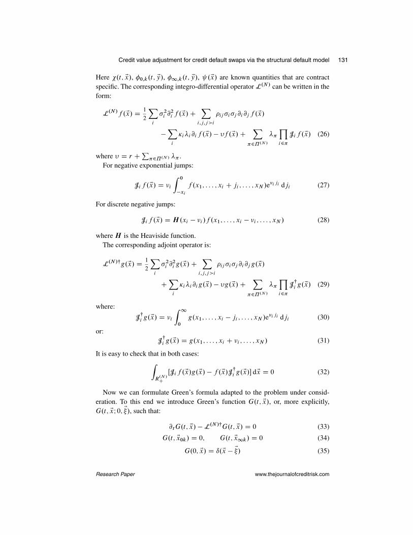
Here .t; Ex/, 0;k.t; Ey/, 1;k.t; Ey/, .Ex/ are known quantities that are contractspecific. The corresponding integro-differential operator L.N/ can be written in theform:
L.N/f .Ex/ D 1
2
Xi
�2i @2i f .Ex/C
Xi;j;j>i
�ij�i�j @i@jf .Ex/
�Xi
�i�i@if .Ex/ � �f .Ex/CX
�2˘ .N /
��Yi2�
Jif .Ex/ (26)
where � D r C P�2˘ .N / �� .
For negative exponential jumps:
Jif .Ex/ D �i
Z 0
�xi
f .x1; : : : ; xi C ji ; : : : ; xN /e�iji dji (27)
For discrete negative jumps:
Jif .Ex/ D H .xi � �i /f .x1; : : : ; xi � �i ; : : : ; xN / (28)
where H is the Heaviside function.The corresponding adjoint operator is:
L.N/�g.Ex/ D 1
2
Xi
�2i @2i g.Ex/C
Xi;j;j>i
�ij�i�j @[email protected]/
CXi
�i�[email protected]/ � �g.Ex/CX
�2˘ .N /
��Yi2�
J�i g.Ex/ (29)
where:
J�i g.Ex/ D �i
Z 1
0
g.x1; : : : ; xi � ji ; : : : ; xN /e�iji dji (30)
or:J�i g.Ex/ D g.x1; : : : ; xi C �i ; : : : ; xN / (31)
It is easy to check that in both cases:ZR
.N /C
ŒJif .Ex/g.Ex/ � f .Ex/J�i g.Ex/� dEx D 0 (32)
Now we can formulate Green’s formula adapted to the problem under consid-eration. To this end we introduce Green’s function G.t; Ex/, or, more explicitly,G.t; ExI 0; E�/, such that:
@tG.t; Ex/ � L.N/�G.t; Ex/ D 0 (33)
G.t; Ex0k/ D 0; G.t; Ex1k/ D 0 (34)
G.0; Ex/ D ı.Ex � E�/ (35)
Research Paper www.thejournalofcreditrisk.com
132 A. Lipton and A. Sepp
Integration by parts yields:
U.0; E�/ DZR
.N /C
.Ex/G.T; Ex/ dEx CXk
Z T
0
ZR
.N �1/C
0;k.t; Ey/gk.t; Ey/ dt d Ey
�Z T
0
ZR
.N /C
.t; Ex/G.t; Ex/ dt dEx(36)
where:gk.t; Ey/ D @kG
�t; x1; : : : ; 0
k; : : : ; xN
�(37)
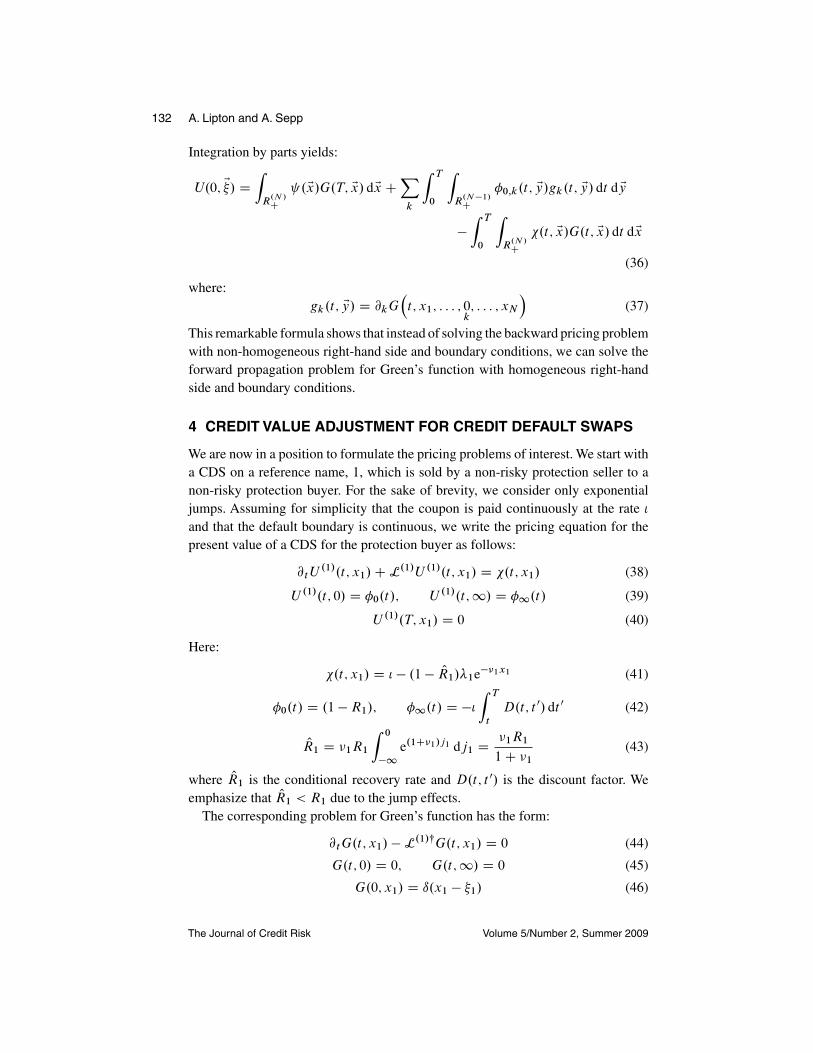
This remarkable formula shows that instead of solving the backward pricing problemwith non-homogeneous right-hand side and boundary conditions, we can solve theforward propagation problem for Green’s function with homogeneous right-handside and boundary conditions.
4 CREDIT VALUE ADJUSTMENT FOR CREDIT DEFAULT SWAPS
We are now in a position to formulate the pricing problems of interest. We start witha CDS on a reference name, 1, which is sold by a non-risky protection seller to anon-risky protection buyer. For the sake of brevity, we consider only exponentialjumps. Assuming for simplicity that the coupon is paid continuously at the rate and that the default boundary is continuous, we write the pricing equation for thepresent value of a CDS for the protection buyer as follows:
@tU.1/.t; x1/C L.1/U .1/.t; x1/ D .t; x1/ (38)
U .1/.t; 0/ D 0.t/; U .1/.t;1/ D 1.t/ (39)
U .1/.T; x1/ D 0 (40)
Here:
.t; x1/ D � .1 � OR1/�1e��1x1 (41)
0.t/ D .1 �R1/; 1.t/ D � Z T
t
D.t; t 0/ dt 0 (42)
OR1 D �1R1
Z 0
�1e.1C�1/j1 dj1 D �1R1
1C �1(43)
where OR1 is the conditional recovery rate and D.t; t 0/ is the discount factor. Weemphasize that OR1 < R1 due to the jump effects.
The corresponding problem for Green’s function has the form:
@tG.t; x1/ � L.1/�G.t; x1/ D 0 (44)
G.t; 0/ D 0; G.t;1/ D 0 (45)
G.0; x1/ D ı.x1 � �1/ (46)
The Journal of Credit Risk Volume 5/Number 2, Summer 2009

Credit value adjustment for credit default swaps via the structural default model 133
When parameters are constant, this problem can be solved via the direct and inverseLaplace transform (see Lipton (2002); Sepp (2004)).
The direct Laplace transform G.t; x1/ ! OG.p; x1/ yields:
12�21
OGx1x1C �1�1 OGx1
� .v1 C p/ OGC�1�1
Z 1
0
OG.p; x1 C j1/e��1j1 dj1 D �ı.x1 � �1/ (47)
OG.p; 0/ D 0; OG.p;1/ D 0 (48)
The corresponding forward characteristic equation has the form:
12�21
2 C �1�1 � .v1 C p/ � �1�1
� �1 D 0 (49)
This equation has three roots of which two are positive and one negative. We denotethem by � i .
The function OG.p; x1/ has the form:
OG.p; x1/
D(C3e� 3.x1��1/; x1 > �1
D1e 1�1 Œe� 1x1 � e� 3x1 �CD2e 2�1 Œe� 2x1 � e� 3x1 �; x1 < �1
(50)
where:
D1 D � 2
�21
.�1 C 1/
. 1 � 2/. 1 � 3/ ; D2 D � 2
�21
.�1 C 2/
. 2 � 1/. 2 � 3/
C3 D 2
�21
�.e. 1� 3/� � 1/.�1 C 1/
. 1 � 2/. 1 � 3/ C .e. 2� 3/� � 1/.�1 C 2/
. 2 � 1/. 2 � 3/�
9>>>=>>>;(51)
The inverse Laplace transform yieldsG.t; x1/. We use the Stehfest algorithm andwrite:
G.t; x1/ D ln 2
t
NXkD1
.�1/k StNk OG�k
ln 2
t; x1
�(52)
where StNk are the Stehfest coefficients (Stehfest (1970)). We typically chooseN D 20. For small t , inversion can be numerically unstable unless computationis performed with high accuracy. Once G.t; x1/ is known, all the relevant instru-ments, including CDSs, equity options, etc, can be evaluated without too mucheffort. In Figure 1 on the next page, we show G.t; x1/ for a model with representa-tive parameters at t D 1Y; 5Y; 10Y.
When parameters are time dependent we need to use numerical methods in orderto solve the pricing problem. Time and space are discretized in the usual way.A judicious combination of finite differences for partial and ordinary differentialequations allows us to build a fast and accurate numerical scheme. Only the integral
Research Paper www.thejournalofcreditrisk.com

134 A. Lipton and A. Sepp
FIGURE 1 Analytically computed probability density function for x.t/ conditional on nodefault for the constant parameter case: � D 0.15, � D 2.5%, � D 10%, r D 0, (a) � D 5.0and (b) � D 10.0 exponential jump.
0
0.01
0.02
0.03
0.04
x
1Y
5Y
10Y
0 0.1 0.2 0.3 0.4 0.5 0.6
1Y
5Y
10Y
0
0.01
0.02
0.03
0.04
0 0.1 0.2 0.3 0.4 0.5 0.6
x
(a)
(b)
term requires special treatment, the rest of the scheme is standard (see, for example,Lipton (2001)). Specifically, let:
I�.x/ D �
Z 0
�xf .x C j /e�j dj D �
Z x
0
e��.x�y/f .y/ dy (53)
We can then calculate I� recursively on the spatial grid:
I�.x/ D e��ıxI�.x � ıx/C 1 � .1C �ıx/e��ıx
�ıxf .x � ıx/
C �1C �ıx C e��ıx
�ıxf .x/ (54)
The Journal of Credit Risk Volume 5/Number 2, Summer 2009

Credit value adjustment for credit default swaps via the structural default model 135
with I�.0/ D 0 (Lipton and Sepp (2009)). This is a special trick for exponentialjumps – it does not work for more familiar Gaussian jumps. For discrete jumps asimple interpolation routine is sufficient.
Alternatively, we can use the discrete Fourier transform (DFT) to solve the pricingproblem. Without going into detail, we present the corresponding method symboli-cally. In this method, we expand the computational domain and calculate one timestep evolution by applying the DFT algorithm twice and write:
U .1/.t � ıt; �/ D P.IFFT.FFT.U .1/.t; x//ˇ FFT.G.t; xI t � ıt; �//// (55)
where FFT and IFFT stand for the directional and inverse FFT, respectively, ˇdenotes element-wise multiplication and P denotes projection on the positive semi-axis. The algorithm is made feasible by the fact that FFT.G.t; xI t � ıt; �// can becomputed analytically (Lipton et al (2007)).
For a CDS on a reference name, 1, which is sold by a risky protection seller, 2, toa non-risky protection buyer, we write the pricing equation as follows:
@tU.2/.t; x1; x2/C L.2/U .2/.t; x1; x2/ D .t; x1; x2/ (56)
U .2/.t; 0; x2/ D 0;1.t; x2/; U .2/.t;1; x2/ D 1;1.t; x2/
U .2/.t; x1; 0/ D 0;2.t; x1/; U .2/.t; x1;1/ D 1;2.t; x1/
)(57)
U .2/.T; x1; x2/ D 0 (58)
Here:
.t; x1; x2/
D � �f1g�1.t; x1; x2/ � �f2g�2.t; x1; x2/ � �f1;2g�1;2.t; x1; x2/ (59)
�1.t; x1; x2/ D .1 � OR1/e��1x1
�2.t; x1; x2/ D QU .1/.t; x1/e��2x2
)(60)
�1;2.t; x1; x2/ D .1 � OR1/e��1x1.1 � e��2x2/
C �1e��2x2
Z 0
�x1
QU .1/.t; x1 C j1/e�1j1 dj1
C .1 � OR1/ OR2e��1x1��2x2 (61)
QU .1/.t; x1/ D OR2U .1/C .t; x1/C U .1/� .t; x1/ (62)
0;1.t; x2/ D 1 �R1; 1;1.t; x2/ D � Z T
t
D.t; t 0/ dt 0 (63)
0;2.t; x1/ D R2U.1/C .t; x1/C U .1/� .t; x1/; 1;2.t; x1/ D U .1/.t; x1/ (64)
and xC D max.x; 0/, x� D min.x; 0/. We define CVA as the difference betweenU .1/ and U .2/:
CVA D U .1/ � U .2/ (65)
Research Paper www.thejournalofcreditrisk.com
136 A. Lipton and A. Sepp
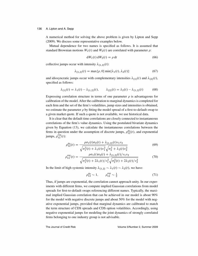
A numerical method for solving the above problem is given by Lipton and Sepp(2009). We discuss some representative examples below.
Mutual dependence for two names is specified as follows. It is assumed thatstandard Brownian motions W1.t/ and W2.t/ are correlated with parameter �:
dW1.t/ dW2.t/ D � dt (66)
collective jumps occur with intensity �f1;2g.t/:
�f1;2g.t/ D maxf�; 0g minf�1.t/; �2.t/g (67)
and idiosyncratic jumps occur with complementary intensities �f1g.t/ and �f2g.t/,specified as follows:
�f1g.t/ D �1.t/ � �f1;2g.t/; �f2g.t/ D �2.t/ � �f1;2g.t/ (68)
Expressing correlation structure in terms of one parameter � is advantageous forcalibration of the model. After the calibration to marginal dynamics is completed foreach firm and the set of the firm’s volatilities, jump sizes and intensities is obtained,we estimate the parameter � by fitting the model spread of a first-to-default swap toa given market quote. If such a quote is not available, we use historical data.
It is clear that the default time correlations are closely connected to instantaneouscorrelations of the firm’s value dynamics. Using the postulated bivariate dynamicsgiven by Equation (13), we calculate the instantaneous correlations between thefirms in question under the assumption of discrete jumps, �dis
12.t/, and exponentialjumps, �exp
12 .t/:
�dis12.t/ D ��1.t/�2.t/C �f1;2g.t/�1�2q
�21 .t/C �1.t/�21
q�22 C �2.t/�
22
(69)
�exp12 .t/ D ��1.t/�2.t/C �f1;2g.t/=�1�2q
�21 .t/C 2�1.t/=�21
q�22 .t/C 2�2.t/=�
22
(70)
In the limit of high systemic intensity �f1;2g � �1.t/ � �2.t/, we have:
�dis12 � 1; �
exp12 � 1
2(71)
Thus, if jumps are exponential, the correlation cannot approach unity. In our exper-iments with different firms, we compute implied Gaussian correlations from modelspreads for first-to-default swaps referencing different names. Typically, the maxi-mal implied Gaussian correlation that can be achieved in our model is about 90%for the model with negative discrete jumps and about 50% for the model with neg-ative exponential jumps, provided that marginal dynamics are calibrated to matchthe term structure of CDS spreads and CDS option volatilities. Accordingly, usingnegative exponential jumps for modeling the joint dynamics of strongly correlatedfirms belonging to one industry group is not advisable.
The Journal of Credit Risk Volume 5/Number 2, Summer 2009

Credit value adjustment for credit default swaps via the structural default model 137
TABLE 1 Market data for December 8, 2009.
XYZ ZYX
s.0/ 36.49 8.47L.0/ 604.11 353.07R 40% 40%l.0/ 241.64 141.22a.0/ 278.13 149.70� 0.1406 0.0582Jump size 0.1406 0.0582Jump size 0.0703 0.0291� 0.0262 0.0113
TABLE 2 CDS spread , survival probability Q, and the values of the default leg and therisky annuity for XYZ and ZYX.
� (%) Q (%) DL RA‚ …„ ƒ ‚ …„ ƒ ‚ …„ ƒ ‚ …„ ƒT XYZ ZYX XYZ ZYX XYZ ZYX XYZ ZYX
1Y 1.05 2.86 98.3 95.3 0.0104 0.0279 0.991 0.9772Y 1.18 2.71 96.1 91.4 0.0232 0.0518 1.963 1.9103Y 1.34 2.57 93.5 88.0 0.0391 0.0721 2.911 2.8074Y 1.47 2.49 90.6 85.6 0.0562 0.0915 3.832 3.6705Y 1.60 2.48 87.4 81.4 0.0754 0.1117 4.722 4.5016Y 1.61 2.43 85.0 78.6 0.0901 0.1286 5.584 5.3007Y 1.62 2.38 82.7 75.9 0.1032 0.1446 6.422 6.0738Y 1.63 2.36 80.3 73.2 0.1180 0.1609 7.237 6.8179Y 1.64 2.34 78.0 70.6 0.1318 0.1766 8.029 7.537
10Y 1.65 2.33 75.8 68.0 0.1451 0.1919 8.799 8.229
5 AN EXAMPLE OF MODEL CALIBRATION AND CVA VALUATION
For illustration, we use market data for two representative financial institutions:XYZ and ZYX. In Table 1 we provide a market data snapshot for December 8,2009; it is used to calculate the initial absolute and relative asset values v.0/ and�. In Table 2 we provide the term structure of CDS spreads for XYZ and ZYX,their survival probabilities implied from these spreads via a reduced-form modelwith piecewise constant hazard rate and the corresponding default leg and riskyannuity (RA) (CL D RA). For details of this procedure see, for example, Jarrowand Turnbull (1995). For simplicity, we assume quarterly coupon payments and adiscount factor of 1.
We compare jump-diffusion models with discrete and exponential jumps andconsider two choices for the jump sizes. First, we set the expected jump size to
Research Paper www.thejournalofcreditrisk.com

138 A. Lipton and A. Sepp
FIGURE 2 Spreads (right axis) and calibrated jump intensities (left axis) for (a) XYZ and(b) ZYX.
0
5
10
15
20
25
30
35
0
0.2
0.4
0.6
0.8
1.0
1.2
1.4
1.6
1.8
ld1
ld2
le1
le2
Spread
0
10
20
30
40
50
60
70
80
Time
0
0.5
1.0
1.5
2.0
2.5
3.0
3.5
ld1
ld2
le1
le2
Spread
0 1 2 3 4 5 6 7 8 9 10
Sp
rea
d (
%)
Jum
p in
ten
sity
(%
)
(a)
(b)
Sp
rea
d (
%)
Jum
p in
ten
sity
(%
)
T ime0 1 2 3 4 5 6 7 8 9 10
the initial relative value of the firm, so that � � �1 D x.0/ in the model withdiscrete jumps and � � 1=�1 D x.0/ in the model with exponential jumps. Second,we set the jump amplitude to half the previous choice: � � �2 D 1
2x.0/ and
� � 1=�2 D 12x.0/, respectively. The asset volatility � is chosen via Equation (9) in
such a way that the diffusion fraction of equity volatility is 20%. We assume discreteweekly default monitoring. We use a finite-difference solver for model calibrationand counterparty charge evaluation.
All in all we have four different models for each firm. Each of these models iscalibrated to the term structure of CDS spreads given in Table 2 on the precedingpage using forward induction. Following this we use the abbreviations le1 and le2for the model with exponential jumps and ld1 and ld2 for the model with discretejumps, respectively.
The Journal of Credit Risk Volume 5/Number 2, Summer 2009

Credit value adjustment for credit default swaps via the structural default model 139
FIGURE 3 The probability density function of the stochastic driver x.t/ conditional onno default: (a) XYZ; (b) ZYX.
0
0.01
0.02
0.03
0.04
0.05
0.06
0.07
0.08
1Y
5Y
10Y
0
0.02
0.04
0.06
0.08
0.10
0.12
0.14
0.16
0.18
1Y
5Y
10Y
x0 0.1 0.2 0.3 0.4 0.5
(a)
(b)
x0 0.05 0.10 0.15 0.20 0.25
In Figure 2 on the facing page we show calibrated intensities. We see that whenthe jump size is large, � D x.0/, the first jump leads to the crossing of the defaultbarrier with high probability for both stochastic and deterministic jumps, so thatjump intensities are close in both cases. For the smaller jump size, the model withexponential jumps has a higher intensity rate because exponential jumps have highervariance, and thus the model expects the jumps to be more frequent in order to matchmarket data.
In Figure 3 we show the implied density of the driver x.t/ for the calibrated modelwith large exponential jumps at t D 1Y; 5Y; 10Y. We see that even for t D 1Y thereis a possibility of default in the short term.
In Figure 4 on the next page we show the implied lognormal CDS option volatilityfor a one-year payer option on a five-year CDS contract calculated via a version of
Research Paper www.thejournalofcreditrisk.com

140 A. Lipton and A. Sepp
FIGURE 4 Black CDS option volatility for a one-year option on a five-year CDS: (a) XYZ;(b) ZYX.
0
20
40
60
80
100
120
80 100 120 140 160 180
ld1
ld2
le1
le2
ld1
ld2
le1
le2
Moneyness (%)
80 100 120 140 160 180
Moneyness (%)
Vol
atili
ty (%
)
0
20
40
60
80
100
120
Vol
atili
ty (%
)
(a)
(b)
the Black futures formula (see, for example, Hull and White (2003); Schönbucher(2004)). This formula assumes that the five-year spread at the option expiry islognormal with volatility � . We plot the model implied volatility as a function ofthe moneyness, K=f , where f is the forward CDS spread at option expiry. Weobserve that the model implied lognormal volatility � exhibits a positive skew. Thiseffect is in line with the fact that option market makers charge an extra premium forout-of-the-money CDS options, because the spread volatility is expected to increasewhen the spread itself increases. Comparing models with different jump sizes, wesee that when the jump size is large, the first jump leads to the crossing of the defaultbarrier with high probability, so the spread volatility is low; when the jump size issmall, the asset value is expected to have several jumps before crossing the defaultbarrier, which results in higher spread volatility. Comparing models with different
The Journal of Credit Risk Volume 5/Number 2, Summer 2009
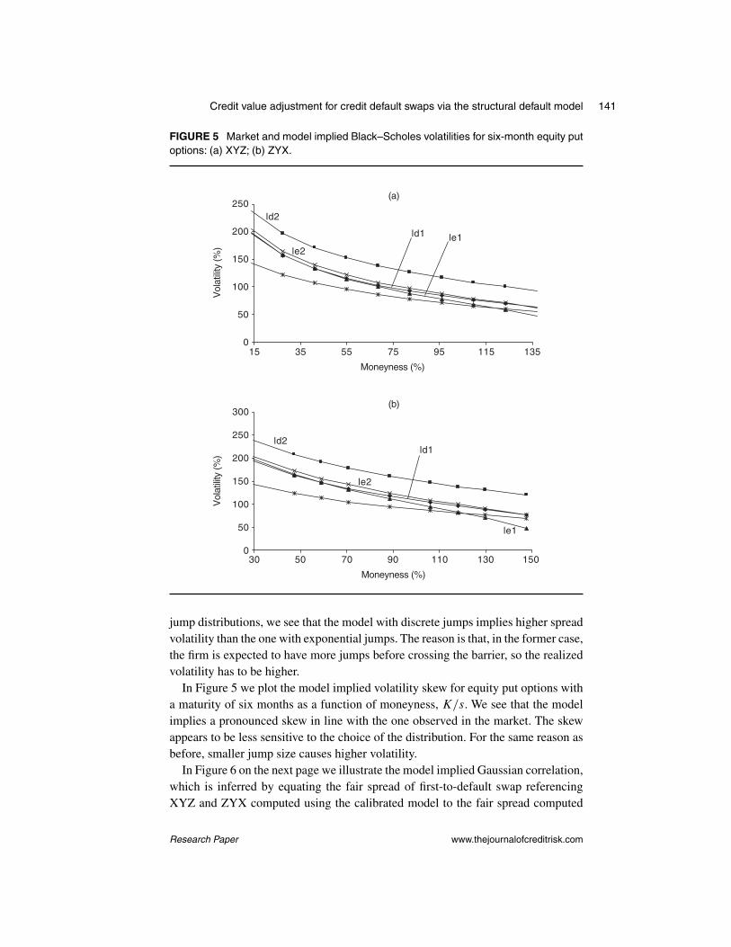
Credit value adjustment for credit default swaps via the structural default model 141
FIGURE 5 Market and model implied Black–Scholes volatilities for six-month equity putoptions: (a) XYZ; (b) ZYX.
15 35 55 75 95 115 135
ld1
ld2
le1le2
ld1ld2
le1
le2
Moneyness (%)
Vol
atili
ty (%
)
0
50
100
150
200
250(a)
(b)
15030 50 70 90 110 130
Moneyness (%)
Vol
atili
ty (%
)
0
50
100
150
200
250
300
jump distributions, we see that the model with discrete jumps implies higher spreadvolatility than the one with exponential jumps. The reason is that, in the former case,the firm is expected to have more jumps before crossing the barrier, so the realizedvolatility has to be higher.
In Figure 5 we plot the model implied volatility skew for equity put options witha maturity of six months as a function of moneyness, K=s. We see that the modelimplies a pronounced skew in line with the one observed in the market. The skewappears to be less sensitive to the choice of the distribution. For the same reason asbefore, smaller jump size causes higher volatility.
In Figure 6 on the next page we illustrate the model implied Gaussian correlation,which is inferred by equating the fair spread of first-to-default swap referencingXYZ and ZYX computed using the calibrated model to the fair spread computed
Research Paper www.thejournalofcreditrisk.com

142 A. Lipton and A. Sepp
FIGURE 6 Implied Gaussian correlations for different instantaneous correlation specifi-cations: (a) � D 0.5; (b) � D 0.99.
0
20
40
60
80
100
120
ld1
ld2
le1
0
20
40
60
80
100
120
le2
Time
0 1 2 3 4 5 6 7 8 9 10
(%)
(%)
ld1
ld2
le1
le2
Time
0 1 2 3 4 5 6 7 8 9 10
(a)
(b)
using the Gaussian copula with an appropriate correlation. We consider two choicesfor the correlation parameter: � D 0:5 and � D 0:99 (see Equations (66) and (67)).We see that, in line with Equation (69), the model with exponential jumps produceslower implied correlation than the one with discrete jumps. In general the correlationis smaller when the jumps are smaller; however, this effect is less pronounced forthe model with discrete jumps.
In Figure 7 on the facing page we show CVA for par CDSs with XYZ as thereference name and ZYX as the protection seller as a function of maturity using CDSspreads from Table 2 on page 137 and two model correlation parameters: � D 0:5
and � D 0:99. We show CVA normalized by the present value of the default leg ofthe corresponding CDSs. We observe the following effects. First, higher correlation
The Journal of Credit Risk Volume 5/Number 2, Summer 2009

Credit value adjustment for credit default swaps via the structural default model 143
FIGURE 7 Credit value adjustment for CDSs on XYZ underwritten by ZYX normalized bythe value of the default leg for different instantaneous correlation specifications: (a) � D0:5; (b) � D 0.99.
ld1
ld2
le1
le2
ld1
ld2
le1
le2
Time
0 1 2 3 4 5 6 7 8 9 10
Time
0 1 2 3 4 5 6 7 8 9 10
(a)
(b)
CV
A (
%)
CV
A (
%)
0
5
10
15
20
25
0
10
20
30
40
50
60
results in higher CVA, because, conditional on protection seller default, the lossof protection is expected to be higher. Second, higher jump size results in higherCVA, because the model with higher jumps implies higher correlation (see Figure 5on page 141). Third, discrete jumps result in higher CVA than exponential jumps,because the former imply higher correlation and higher CDS spread volatility. Wesee that for moderate correlation, � D 0:5, the model with large discrete jumpsimplies CVA of the order of 10–15% of the present value of the default leg, whilefor high correlation, � D 0:99, its magnitude grows to 30–40% of the default leg.
In Figure 8 on the next page we show CVA for par CDSs with ZYX as the referencename and XYZ as the protection seller. We observe the same effects as before. Wealso see that CVA is not symmetric. It might be expected that a riskier protection
Research Paper www.thejournalofcreditrisk.com

144 A. Lipton and A. Sepp
FIGURE 8 Credit value adjustment for CDSs on ZYX underwritten by XYZ normalized bythe value of the default leg for different instantaneous correlation specifications: (a) � D0.5; (b) � D 0.99.
ld1 ld2
le1
le2
ld1 ld2
le1
le2
Time
0 1 2 3 4 5 6 7 8 9 10
Time0 1 2 3 4 5 6 7 8 9 10
(a)
(b)
CV
A (
%)
CV
A (
%)
0
2
4
6
8
12
10
0
5
10
15
20
25
30
seller implies higher CVA; however, for high correlation the opposite effect mightbe observed. The reason being that in cases when a safer protection seller defaultsright before the riskier reference name, the realized loss is higher than that in theopposite case.
6 CONCLUSIONS
We present a multi-dimensional extension of the Merton (1974) model, with thejoint dynamics of asset values driven by a multi-dimensional jump-diffusion process.Applying FFT- and PIDE-based methods, we develop a forward induction procedure
The Journal of Credit Risk Volume 5/Number 2, Summer 2009

Credit value adjustment for credit default swaps via the structural default model 145
for the model calibration and a backward induction procedure for the valuation ofcredit instruments in one and two dimensions.
We consider two types of jump size distributions: namely, negative discrete andnegative exponential. We show that both jump specifications result in an adequate fitto the market data for individual names. However, for the joint bivariate dynamics,the model with exponential negative jumps produces a noticeably lower correlationbetween names than the model with discrete negative jumps. Based on this obser-vation and given a high level of the default correlation among financial institutions(above 50%), the model with constant negative jumps, despite being simple, seemsto provide a more realistic description of default correlations and, thus, is prefer-able for the evaluation of CVA. Our empirical analysis shows that CVA is largelydetermined by the correlation between the reference name and the protection seller,and their spread volatility, with higher correlation and volatility resulting in higheradjustment. Thus, by accounting for both of these factors, the model provides arobust estimate of the counterparty risk.
REFERENCES
Black, F., and Cox, J. (1976).Valuing corporate securities: some effects of bond indentureprovisions. Journal of Finance 31, 351–367.
Blanchet-Scalliet, C., and Patras, F. (2008). Counterparty risk valuation for CDS.WorkingPaper.
Brigo, D., and Chourdakis, K. (2008). Counterparty risk for credit default swaps: impactof spread volatility and default correlation. Research paper, FitchSolutions.
Crepey, S., Jeanblanc, M., and Zargari, B. (2009). CDS with counterparty risk in a Markovchain copula model with joint defaults.Working Paper, Université de Lyon and Universitéde Nice.
Finger, C., Finkelstein, V., Pan, G., Lardy, J., Ta, T., and Tierney, J. (2002). CreditGradestechnical document, RiskMetrics Group.
Gregory, J. (2009). Being two-faced over counterparty credit risk. Risk 22(2), 86–90.Haworth, H., Reisinger, C., and Shaw, W. (2006). Modelling bonds and credit default
swaps using a structural model with contagion. Working Paper, Oxford University.Hilberink, B., and Rogers, L. C. G. (2002). Optimal capital structure and endogenous
default. Finance and Stochastics 6, 237–263.Hull, J., and White, A. (2001).Valuing credit default swaps II: modeling default correlations.
Journal of Derivatives 8(3), 12–22.Hull, J., and White, A. (2003). The valuation of credit default swap options. Journal of
Derivatives 10(3), 40–50.Hyer, T., Lipton, A., Pugachevsky, D., and Qui, S. (1998). A hidden-variable model for
risky bonds. Working Paper, Bankers Trust.Jarrow, R., and Turnbull, T. (1995). Pricing derivatives on financial securities subject to
credit risk. Journal of Finance 50(1), 53–85.Jarrow, R., and Yu, J. (2001). Counterparty risk and the pricing of defaultable securities.
Journal of Finance 56(5), 1,765–1,800.Kiesel, R., and Scherer, M. (2007). Dynamic credit portfolio modelling in structural models
with jumps. Working Paper, Ulm University and TU Munich.
Research Paper www.thejournalofcreditrisk.com

146 A. Lipton and A. Sepp
Leung, S., and Kwok,Y. (2005).Credit default swap valuation with counterparty risk.KyotoEconomic Review 74(1), 25–45.
Li, D. (2000).On default correlation: a copula approach.Journal of Fixed Income 9, 43–54.Lipton, A. (2001). Mathematical Methods for Foreign Exchange: A Financial Engineer’s
Approach. World Scientific.Lipton, A. (2002). Assets with jumps. Risk 15(9), 149–153.Lipton, A., Song, J., and Lee, S. (2007). Systems and methods for modeling credit risks
of publicly traded companies. US Patent 2007/0027786 A1.Lipton, A., and Sepp, A. (2009). Multi-factor structural default models and their applica-
tions. Working Paper, Bank of America Merrill Lynch (in preparation).Marshall, A.W., and Olkin, I. (1967). A multivariate exponential distribution. Journal of the
American Statistical Association 2, 84–98.Merton, R. (1974). On the pricing of corporate debt: the risk structure of interest rates.
Journal of Finance 29, 449–470.JPMorgan (1997). CreditMetrics technical document.Pykhtin, M., and Zhu, S. (2006). Measuring counterparty credit risk for trading products
under Basel II. In Basel II Handbook, Ong, M. (ed.). Risk Books, London.Rubinstein, M. (1983). Displaced diffusion option pricing. Journal of Finance 38(1), 213–
217.Sato, K. (1999). Lévy Processes and Infinitely Divisible Distributions. Cambridge Univer-
sity Press.Schönbucher, P. (2004). A measure of survival. Risk 17(8), 79–85.Sepp, A. (2004). Analytical pricing of double-barrier options under a double-exponential
jump diffusion process: applications of Laplace transform. International Journal ofTheoretical and Applied Finance 2, 151–175.
Sepp, A. (2006). Extended CreditGrades model with stochastic volatility and jumps.Wilmott Magazine September, 50–62.
Stamicar, R., and Finger, C. (2006). Incorporating equity derivatives into the CreditGradesmodel. The Journal of Credit Risk 2(1), 1–20.
Stehfest, H. (1970). Algorithm 368 numerical inversion of Laplace transforms. Communi-cations of the ACM 13, 479–490 (erratum: 13, 624).
Turnbull, S. (2005).The pricing implications of counterparty risk for non-linear credit prod-ucts. The Journal of Credit Risk 4(1), 117–133.
Zhou, C. (2001a). The term structure of credit spreads with jump risk. Journal of Bankingand Finance 25, 2,015–2,040.
Zhou, C. (2001b). An analysis of default correlations and multiple defaults. Review ofFinancial Studies 14(2), 555–576.
The Journal of Credit Risk Volume 5/Number 2, Summer 2009


![Bloom Berg] Credit Default Swaps](https://static.fdocuments.in/doc/165x107/577d25391a28ab4e1e9e5000/bloom-berg-credit-default-swaps.jpg)