Credit Ratings: Strategic Issuer Disclosure and Optimal

Screening∗

Jonathan Cohn† Uday Rajan‡ Gunter Strobl§

July 18, 2018

Abstract

We study a model in which an issuer can manipulate information obtained by a credit

rating agency (CRA). Better CRA screening reduces the likelihood of a high rating, but

increases the value of a rated security. We find that improving the prior quality of assets

can have no effect on the quality of a high-rated security, as low-type issuers manipulate

more often in equilibrium. The issuer’s response to anticipated CRA screening can either

amplify or attenuate the effects on accuracy of increased penalties for ratings errors. Our

model highlights the importance of strategic issuer disclosure in recent ratings failures.

∗This paper is a substantially revised version of a previous paper with the same title. We thank AndresAlmazan, Aydogan Altı, Taylor Begley, Sugato Bhattacharyya, Patrick Bolton, Matthieu Bouvard, EdwigeCheynel, Jason Donaldson, Sivan Frenkel, John Griffin, David Hirshleifer, Beatriz Mariano, Christian Opp,Marcus Opp, Amiyatosh Purnanandam, David Scharfstein, Martin Schmalz, Joel Shapiro, Sheridan Titman,Yizhou Xiao, and participants at seminars at Boston College, Boston University, CUHK, Duke, Georgia Tech,IDC Herzliya, Indiana, Michigan, NYU, Tel Aviv, UT Austin, UC Davis, UC Irvine, Washington U, and theCredit Ratings, AFA, EFA, FIRS, Erasmus Credit, Oxford Financial Intermediation, and LSE Paul Woolleyconferences for helpful comments. Errors and omissions remain our responsibility.†McCombs School of Business, University of Texas, Austin; jonathan.cohn@mccombs.utexas.edu‡Stephen M. Ross School of Business, University of Michigan, Ann Arbor; urajan@umich.edu§Frankfurt School of Finance and Management; g.strobl@fs.de

Disclosure Statement: Jonathan Cohn

Jonathan Cohn has nothing to disclose.

Disclosure Statement: Uday Rajan

Uday Rajan has nothing to disclose.

Disclosure Statement: Gunter Strobl

Gunter Strobl has nothing to disclose.

1 Introduction

The failure of credit ratings to predict defaults of mortgage-backed securities in the lead-

up to the financial crisis raises questions about the role of credit rating agencies (CRAs)

in the economy. In principle, these “information intermediaries” create value by producing

information in the form of ratings that allows investors to more accurately price assets.

However, incentive problems may distort ratings and hence their usefulness. There has been

much focus on CRAs inflating ratings of mortgage-backed securities in the pre-crisis era.

However, an under-explored facet of the ratings process is the reliance of CRAs on issuers

for much of the information on which they base their ratings.

We construct a theoretical model to investigate the implications of issuers’ ability to

distort information used to rate securities. An issuer with a low-quality asset can, at a cost,

attempt to induce a favorable rating by manipulating a CRA’s information. The CRA, for its

part, chooses how much to invest in screening to reduce the probability that such manipulation

is successful. We show that these two simple decisions interact in complex ways. The CRA,

which cares about ratings accuracy, increases its screening intensity when it assigns a higher

probability to manipulation by the issuer. However, the issuer may manipulate either more

or less frequently when it expects the CRA to screen more intensely. The issuer’s behavior

can therefore either amplify or attenuate the effects of efforts to improve ratings quality by

penalizing CRAs more for ratings errors.

We show that improvements in fundamental asset quality may not translate into improve-

ments in the quality of securities actually sold. Before the late 1990s, subprime mortgages

were thought of as low-quality assets. Perceptions of the quality of securities backed by these

mortgages improved over the next several years. However, the crisis revealed that a large

proportion of poor-quality loans had, in fact, been previously issued. Our model explains this

finding by showing that a low-quality issuer increases its misreporting as the prior belief over

quality improves. Information manipulation of this type is likely to be especially important

for relatively new or complex assets such as mortgage-backed securities.

Many commentators have argued that CRAs were negligent - and possibly complicit - in

the build-up to the financial crisis. We are by no means attempting to diminish the culpability

of CRAs. However, our model puts some focus back on the role of the issuer in misleading

both CRAs and investors.1 Our results point to the need to account for issuer behavior

1In a written statement before the US SEC on November 21, 2002, Raymond W. McDaniel, President of

1

when using observed ratings accuracy to assess CRA diligence. We also show that penalizing

issuers for distorting information can increase ratings accuracy by improving CRA screening

incentives, even if these penalties are too small to have much effect on issuer behavior.

The issuer in our model has either a high-quality (positive NPV) or low-quality (negative

NPV) project against which it can sell a financial claim. The issuer decides whether or not

to apply for a rating. If it seeks a rating, the CRA subsequently observes a signal of project

quality and assigns the security a high or low rating consistent with its signal.2 The issuer

pays a rating fee to the CRA if a high rating is assigned. It then sells its security to investors,

who form rational expectations and break even on average. Finally, the project pays off. We

first treat the rating fee as exogenous and then later endogenize it as the solution to a Nash

bargaining game between the issuer and the CRA.

If project quality is high, the CRA observes a high signal. If project quality is low,

the CRA may observe either a high or low signal. A low-type issuer (i.e., an issuer with a

low-quality project) chooses whether to manipulate the information it reports to the CRA.

The cost of doing so captures both the direct costs of distorting information as well as

expected longer-run costs associated with sanctions for false disclosure and loss of reputation.

Simultaneously, the CRA chooses how much to invest in screening in order to reduce the

likelihood that such manipulation is successful.

Given the information structure of the game, either a low rating or the lack of a rating

reveals the issuer to be the low type. As a low-quality project is negative NPV, an unrated

or low-rated security will not be issued. The price of a high-rated security is the expected

NPV of the underlying project, given the equilibrium strategies of the issuer and CRA. A

high-type issuer always requests a rating since it is guaranteed to receive a high rating. The

low-type issuer may or may not request a rating, but always manipulates if it seeks a rating.3

The issuer’s payoff is the expected revenue from selling its financial claim (which takes into

account the probability of obtaining a high rating), less the rating fee and any manipulation

costs. The CRA’s payoff is the expected fee for a high rating, less the cost of screening and

an expected penalty for a rating error.

Moody’s Investors Service, states “Most issuers operate in good faith and provide reliable information to thesecurities markets, and to us. Yet there are instances where we may not believe that the numbers providedor the representations made by issuers provide a full and accurate story.”

2Our model therefore features a binary type of issuer and binary ratings. Goel and Thakor (2015) rationalizecoarse (i.e., discrete) ratings.

3In the absence of manipulation, the CRA assigns the low type a low rating, so not manipulating isequivalent to not requesting a rating.

2

We show that there are three types of equilibria in the game. When the manipulation

cost is high, the issuer never manipulates. Anticipating this, the CRA does not invest in

screening. When the manipulation cost is low, the low-type issuer always manipulates, and

the CRA invests heavily in screening. At a moderate manipulation cost, the low-type issuer

mixes between manipulating and not manipulating, and the CRA invests a moderate amount

in screening. We refer to these outcomes as “zero-manipulation,” “full-manipulation,” and

“partial-manipulation” equilibria, respectively.

The key to many of our conclusions lies in two countervailing effects of the anticipated

screening intensity on the low-type issuer’s incentives to manipulate. Increased screening

intensity reduces the probability that the low-type issuer receives a high rating, weakening

the incentive to manipulate. This direct “filtering” effect of increased screening intensity on

incentives is most pronounced when the expected price of a high-rated security is high; that

is, when the screening intensity itself is high. However, increased screening intensity also

increases the price of a high-rated security, which strengthens the incentive to manipulate.

This indirect “price improvement” effect is most pronounced when the probability of success-

ful manipulation is high; that is, when the screening intensity is low. These countervailing

effects produce an inverse U-shaped relationship between the frequency of manipulation and

anticipated screening intensity in a partial-manipulation equilibrium.

The issuer’s response to changes in anticipated screening intensity affects the overall

impact on ratings accuracy of changes in the penalty on the CRA for inaccurate ratings. An

increase in this penalty results in more intense screening; all else equal, this improves ratings

accuracy. The issuer’s response to an increase in expected screening intensity amplifies the

positive effect on ratings accuracy when the penalty is already high, as screening intensity

is high in this case. In contrast, it dampens the effect of increased screening when screening

intensity is low. Thus, increasing sanctions for reporting errors from mild to only moderate

levels may be ineffective at significantly improving ratings quality. On the other hand, small

increases may be sufficient to generate substantial improvements in ratings accuracy when

these penalties are already fairly high.

The model also produces a noteworthy conclusion regarding the quality of a high-rated

security when the average quality of underlying assets improves. In a partial-manipulation

equilibrium, the low-type issuer responds to an increase in the prior belief that the asset is

high quality by manipulating more often, to the point that the average quality of assets for

3

which issuers seek high ratings remains unchanged. Facing the same distribution of assets for

which issuers seek high ratings, the CRA does not change its screening intensity, and thus

the average quality of assets receiving a high rating does not change.

Finally, if the equilibrium features full manipulation, a small increase in the issuer’s

manipulation cost has no effect on its behavior. It can nevertheless impact equilibrium

screening intensity if the fee for a high-rated asset is endogenously set through a bargaining

protocol. In this case, the issuer passes part of the higher expected manipulation cost through

to the CRA in the form of a lower equilibrium fee. This lower fee reduces the benefit to the

CRA of assigning a high rating to a low-quality asset, and results in a higher screening

intensity. Thus, making manipulation more difficult can improve ratings accuracy even if it

does not affect the issuer’s behavior.

Our paper contributes primarily to the literature examining the process by which CRAs

produce information and assign ratings to issuers. Most of the papers in this literature focus

on distortions in the ratings process due to issuers’ ability to “shop” for favorable ratings

(Skreta and Veldkamp, 2009; Bolton, Freixas, and Shapiro, 2012; Sangiorgi and Spatt, 2017)

or CRA incentives to inflate ratings (Mathis, McAndrews, and Rochet, 2009; Fulghieri, Strobl,

and Xia, 2014; Frenkel, 2015; Bouvard and Levy, 2017). Our paper adds to this literature

by accounting for the ability of an issuer to distort the information on which a CRA relies

in evaluating the issuer’s securities and assigning ratings. Our results demonstrate that a

more stringent ratings process can either mitigate or amplify these incentives. The issuer’s

response may therefore either enhance or undermine efforts to improve ratings quality by

lowering the cost of screening or holding CRAs more accountable for ratings errors.

The audit literature has also considered the strategic interaction between a firm and a

certifier (the auditor). For example, Hillegeist (1999), Laux and Newman (2010), and Deng,

Melumad, and Shibano (2012) consider models in which a firm can misreport its type and

the auditor chooses the quality of its own signal. The focus in this literature has been on

the effect of changing auditor liability on overall audit quality.4 An important difference in

the credit ratings context is that, in the audit literature, some to all of the penalties on the

auditor for underperformance represent a direct transfer to investors. This affects the ex ante

value of the security to investors. On the other hand, it is very difficult for investors to win a

lawsuit against credit rating agencies, as the courts have typically held that credit ratings are

4Strobl (2013) considers the effect of audit quality on earnings manipulation, but treats the audit qualityas fixed and observable, in contrast with our approach.

4

opinions protected by free speech (see, e.g., Nagy, 2009). Thus, the penalty incurred by the

CRA in our model represents the cost of reputational loss and possible fines by the regulators,

but is not earned by the investors. In terms of focus, the penalty on the CRA is only one

feature of interest to us, and we also derive interesting comparative static implications from

changing the prior probability of a high-type issuer, the manipulation cost on the issuer, the

technological cost of screening, and the bargaining power of the issuer.5

Finally, our paper is related to the economics of crime literature. Tsebelis (1990) argues

that an enforcement agency optimally responds to an increase in the penalty for crime by

weakening enforcement, undoing the effect of the increased penalty. A similar phenomenon

generally occurs in our setting, with the CRA optimally reducing screening intensity in re-

sponse to an increase in the cost of manipulation. However, as noted, an increase in the cost

of manipulation can actually result in greater screening intensity when the issuer’s incentives

to manipulate are overwhelming and the issuer and CRA bargain over a rating fee upfront.

We also add to this literature by exploring the effects of the cost of enforcement in the form

of CRA screening, showing that an increase in this cost has ambiguous effects on the extent

of issuer misbehavior.

2 Model

An issuer has a project that requires an upfront investment and generates a future cash

flow. The project is high quality with probability η and low quality with probability 1 − η.

The high-quality project has an NPV vh > 0, and the low-quality project has an NPV v` < 0.

The values of η, vh, and v` are common knowledge.

The issuer privately observes the quality of its own project. The issuer has no financial

resources, so if it wishes to undertake the project, it must issue a financial claim backed by

the project. If it does not undertake the project, it obtains a payoff of zero. For convenience,

we refer to an issuer with a high- (low-) quality project as a high- (low-) type issuer. We

normalize vh to 1 and v` to −1.

An issuer wishing to sell a financial claim can obtain a rating from a credit rating agency

5Certification of a strategic agent has been considered in other settings as well. For example, Cohn andRajan (2013) show that the certification by a board of directors of a CEO’s strategic choices can exacerbateagency conflicts due to CEO reputational concerns. Gill and Srgoi (2012) analyze a model where a seller canchoose the stringency of a certification test. As in our model, greater stringency hurts the seller by reducing theprobability of certification but benefits the seller by increasing the price conditional on certification. However,there is no manipulation in their model (i.e., the seller is not strategic).

5

(CRA). The CRA obtains a noisy signal about the type of the project and issues a rating.

Investors observe the rating, update their beliefs about issuer type, and decide whether

they wish to buy the financial claim being issued. Investors are risk-neutral and perfectly

competitive, so if they purchase the claim, they do so at the expected NPV of the project,

given their posterior beliefs.

There are two dates in the model, 0 and 1. The discount rate is normalized to zero. The

sequence of events at date 0 is as follows:

1. The issuer privately observes its type, high or low.

2. Simultaneously,

(i) The issuer chooses whether or not to approach the CRA to request a rating. If

a low-type issuer requests a rating, it further chooses whether or not to take an

unobserved action that we refer to as “manipulating” the information observed by

the CRA (more on the consequences of this decision shortly). Manipulation incurs

a cost m > 0, which captures both upfront costs of distorting or misrepresenting

information presented to the CRA as well as expected longer-run costs associated

with sanctions for false disclosure and loss of reputation.

(ii) The CRA privately chooses a screening intensity α. If the issuer seeks a rating,

the CRA incurs a screening cost kc(α), where k > 0 and c(·) is strictly increasing

and strictly convex. We assume that c(0) = c′(0) = 0, so that in the absence of

screening, both total and marginal costs to the CRA are zero. We also assume

that limα→1 c′(α) = ∞, which ensures that the equilibrium screening intensity is

less than 1.

3. If the issuer does not seek a rating, the game ends. If a rating is sought, the CRA

observes a binary signal of project quality. If project quality is high, then the CRA

observes a high signal. If project quality is low and the issuer did not manipulate the

information observed by the CRA, the CRA observes a low signal. If project quality

is low and the issuer did manipulate the CRA’s information, then the CRA observes a

low signal with probability α and a high signal with probability 1− α.

The CRA then assigns a public rating, rh (“high” rating) or r` (“low” rating),

to the financial claim backed by the project. We assume that the CRA assigns a rating

6

corresponding to its signal. Observe that it cannot be optimal to assign a low rating

when the CRA obtains a high signal, as it only obtains a fee if the rating is high. The

absence of direct rating inflation (assigning a high rating given a low signal) may be

justified by relying on extremely high penalties if the CRA is found to have indulged

in outright fraud (as opposed to merely being incompetent). Observe also that, in our

setting, it cannot be optimal to both have α > 0 and to assign a high rating when a

low signal is obtained, as the same outcome is obtained at lower cost by reducing α

instead.

If the CRA assigns a high rating, the issuer pays a fee f ≥ 0 to the CRA.6 We

take this fee as exogenously given in Section 3 and later endogenize it as the outcome

of a bargaining process in Section 4. We assume that this fee is not so large that it

deters all issuance.

4. Investors compute the NPV of the project, given the CRA’s report (rh or r`), their

beliefs about screening intensity α and about the reporting strategy of each type. From

an investor’s perspective, the financial claim is an asset, and sells at a price equal to

its expected NPV. If the security is issued, the project is carried out.

If the project is undertaken, at date 1 all parties find out the type of the project and earn

their respective terminal payoffs. The CRA incurs a penalty λ > 0 if its rating proves to be

incorrect; that is, if a claim with a rating of rh proves to be backed by a low-quality project.7

This penalty captures, in reduced form, the reputational cost of reduced investor confidence

as well as explicit regulatory sanctions and losses from investor lawsuits.8

We consider perfect Bayesian equilibria of the game. Formally, there are three players to

the game: the issuer, the CRA, and investors as a group. Other than the type of the firm

and the actions of the issuer and CRA, all information is common knowledge. Investors form

rational expectations and compete in a perfectly competitive market, so earn zero profits in

6As is standard in the literature, we assume that the issuer only pays the rating fee f if the rating is high.This assumption is consistent with the large literature that has commented on the incentive to inflate ratingsin an issuer-pay model. Qualitatively, many of our results go through if the fee is paid upfront, before therating is issued. Of course, the exact forms of the expressions we exhibit will change.

7In principle, a rating would also be incorrect if a claim with a rating of r` proves to be backed by ahigh-quality project. However, only upward rating errors are possible in our model, so an incorrect rating inour model is “inflated” in the sense that it induces a favorable belief about a low-quality security.

8As an example of these explicit costs, in 2015, Standard & Poor’s reached a settlement with the JusticeDepartment over inflated ratings on mortgage-backed securities over the period 2004–2007, and agreed to pay$1.375 billion. See Department of Justice (2015).

7

expectation. By construction, only a low type obtains a low rating, so a low-rated security

cannot be issued in equilibrium. The price of a high-rated security, p, equals the expected

payoff of the project backing it, given investors’ conjectures regarding the strategies of the

CRA and the issuer. In equilibrium, these conjectures must be correct.

We restrict attention to equilibria that survive the D1 refinement. In such equilibria,

a high-type issuer always requests a rating, ensuring that an unrated security cannot be

issued.9 Thus, in describing equilibrium issuer strategies, we need only specify the strategy

of a low-type issuer. In principle, a low type issuer makes two choices: whether or not to

request a rating and, conditional on requesting a rating, whether or not to manipulate the

CRA’s information. However, requesting a rating but not manipulating guarantees the issuer

a low rating, which reveals the issuer to be the low type and is therefore informationally

equivalent to not requesting a rating. Therefore, to simplify the strategy space, we disallow

the possibility that the low-type issuer can request a rating but not manipulate. Thus, a

low-type issuer may request a rating (and manipulate), not request a rating, or mix between

the two actions. We denote by σ the probability with which the low-type issuer requests a

rating.

The only choice the CRA makes in the game is its level of screening intensity α. Thus,

when the rating fee f is exogenous, a perfect Bayesian equilibrium of the game is represented

by (α, σ), where each player’s strategy maximizes its own payoff, given its own beliefs and

the actions of other parties in the game. When the rating fee is endogenous, it too must be

determined as part of the equilibrium.

We analyze this model in the next two sections. In Section 3, we take the rating fee f

as fixed and solve for the equilibrium (α, σ). Much of the intuition in the paper comes from

analyzing the fixed-fee case. In Section 4, we endogenize the rating fee as the solution to a

Nash bargaining game and solve for the equilibrium, (f, α, σ). We show that in equilibrium

the fee is strictly less than the price of the high-rated security in this case, again ensuring

that the high-type issuer always seeks a rating.

9Absent the D1 refinement, there always exists an equilibrium in which no issuer requests a rating, sup-ported by investors’ beliefs attributing a deviation to the low-type issuer. D1 effectively requires that investorsattribute a deviation to the type that faces a lower cost of deviating. The high type faces a lower cost of re-questing a rating, since the low type must bear the manipulation cost m in order to have a chance of receivinga high rating and issuing a security.

8

3 Fixed Rating Fee

In this section, we take the fee f as exogenous, and solve for the equilibrium (α, σ). We

do so in two steps. First, we analyze the best responses of the CRA and the low-type issuer,

taking the price of a high-rated security, p, as given. We then close the model by imposing

the requirement that p be set so that investors break even in expectation, and solve for the

equilibrium.

3.1 Best responses of CRA and issuer

Consider the CRA’s best response, taking the low-type issuer’s strategy σ as given. Let

σ denote the CRA’s conjecture of σ. The CRA’s expected payoff depends in part on the

quality of the pool of issuers it expects to request a rating. Define ν(σ) = ηη+(1−η)σ as the

probability that the issuer is a high type, conditional on requesting a rating. Note that ν

decreases with σ and can take on values between η (if σ = 1; that is, if all issuers request a

rating) and 1 (if σ = 0; that is, if only high-type issuers request a rating). The total mass

of issuers requesting a rating is given by N(σ) = η + (1 − η)σ. Thus, given σ, the CRA’s

expected payoff is

Ψ(σ) = N(σ) {ν(σ)f + [1− ν(σ)](1− α)(f − λ)− kc(α)} . (1)

The CRA’s objective is to choose α to maximize Ψ. Observe that, as the CRA takes the

low type’s strategy as given, maximizing Ψ is equivalent to maximizing the term in the

parentheses in equation (1). The following lemma characterizes the CRA’s best response.

Proofs of all results are in Appendix A.

Lemma 1. The best response of the CRA satisfies c′(α) = [1− ν(σ)] max{λ−fk , 0

}.

When f < λ, the CRA’s optimal screening intensity increases with σ, as ν(·) is a decreas-

ing function. Intuitively, since the CRA views erroneous ratings as costly, it screens more

intensely when it expects the low-type issuer to manipulate with higher probability. It also

screens more intensely when the cost it ascribes to an erroneous rating, λ, is higher and less

intensely when the fee it receives for rating a security, f , is higher.10

10One may note that when α = 0, it is curious why the rating is still relevant at this point. One can

9

Next, consider the low-type issuer’s best response, taking the CRA’ strategy α and the

anticipated price of a high-rated security p as given. Let α denote the low-type issuer’s

conjecture of α and p the expected price p of a high-rated security. If the low-type issuer

does not request a rating, then its project is revealed to be low quality. Since a low-quality

project is negative NPV, the issuer does not sell an asset in this case, and its payoff is zero.

If, on the other hand, the low-type issuer requests a rating, it bears the manipulation cost

m, and expects to receive a high rating with probability 1 − α. If it obtains a high rating,

it pays a fee f to the CRA and sells its asset at an anticipated price p. If it obtains a low

rating, its payoff is zero. Thus, the low-type issuer’s expected payoff if it requests a rating is

π`(α, p) = (1− α)(p− f)−m. (2)

The following lemma characterizes the low-type issuer’s best response.

Lemma 2. It is a best response for the low-type issuer to request a rating (i.e., set σ = 1) if

(1− α)(p− f) ≥ m, and to not request a rating (i.e., set σ = 0) if (1− α)(p− f) ≤ m.

Note that if (1 − α)(p − f) = m, then any σ ∈ [0, 1] represents a best response for the

low-type issuer. Equilibria in which the low-type issuer mixes between seeking a rating and

not doing so are of particular interest to us in the rest of the paper.

3.2 Price of a high-rated security

Next, we solve for the price of a high-rated security p, given investors’ beliefs about the

issuer’s and CRA’s strategies. To keep notation simple, we assume that investors’ beliefs

coincide with those of the CRA and the issuer (which will be true in equilibrium), so that

α is the investors’ conjecture of α and σ their conjecture of σ. As investors are perfectly

competitive and form rational expectations, the price p must equal the expected value of an

asset, conditional on a high rating. The price, then, must satisfy

p(α, σ) =ν(σ)vh + [1− ν(σ)](1− α)v`ν(σ) + [1− ν(σ)](1− α)

=ν(σ)− [1− ν(σ)](1− α)

ν(σ) + [1− ν(σ)](1− α). (3)

rationalize the existence of the CRA in this case by introducing a third type of issuer with a terrible projectthat has extremely negative NPV (say a Ponzi scheme) and assuming that the CRA adds value because it canperfectly and costlessly screen out the terrible type.

10

Observe that p is decreasing in σ and increasing in α. Holding α fixed, a higher anticipated

probability of manipulation by the low-type issuer implies a worse pool of issuers requesting

a high rating. As α < 1, the pool of issuers that investors expect to survive screening and

receive a high rating also worsens, resulting in a lower expected payoff from a high-rated

asset, and hence a lower price. Similarly, holding σ fixed, a higher anticipated screening

intensity filters out more low-type issuers, improving the expected pool of high-rated assets

and hence increasing the price investors are willing to pay.

3.3 Equilibrium

Let α∗, σ∗, and p∗ denote the equilibrium values of α, σ, and p. In equilibrium it must

be that α = α∗, σ = σ∗, and p = p∗.

Suppose first that the CRA and investors conjecture that the low-type issuer always

requests a rating (i.e., σ = 1). Then, ν = η and the CRA’s best response is α1d=

c′−1(

(1− η) max{λ−fk , 0

}). Accounting for this response, investors set the price of a high-

rated security to p(α1, 1). Given this price and a belief that α = α1, it is a best response

for the low-type issuer to request a rating if m ≤ (1 − α1)(p(α1, 1) − f). The best response

is unique if m < (1 − α1)(p(α1, 1) − f). Thus, if the manipulation cost is sufficiently low,

in equilibrium the low-type issuer always requests a rating, so that σ∗ = 1. We call such an

equilibrium a “full-manipulation” equilibrium.

Next, suppose that the CRA and investors conjecture that the low-type issuer never

requests a rating (i.e., σ = 0). Then, ν = 1, and the CRA’s best response is to set α = 0.

Therefore, the price of a high-rated security is rationally set to 1. For the low-type issuer,

in turn, it is a best response to not request a rating if m ≥ 1 − f . So, if the manipulation

cost is sufficiently high, then the low-type issuer never requests a rating in equilibrium (i.e.,

σ∗ = 0). We call such an equilibrium a “zero-manipulation” equilibrium.

For values of m such that (1−α1)(p(α1, 1)−f) < m < 1−f , no equilibrium in which the

issuer plays a pure strategy (σ∗ = 0 or σ∗ = 1) is sustainable. In this case, the low-type issuer

mixes between requesting and not requesting a rating. For such mixing to be sustainable,

the low-type issuer must be indifferent between the two actions, so that (α∗, σ∗) must satisfy

the condition (1− α∗)(p(α∗, σ∗)− f) = m.

Note that α1 and p(α1, 1) are functions only of exogenous parameters. We can now fully

characterize the equilibrium of the game.

11

Proposition 1. When f < 1 is fixed, the equilibrium is as follows:

(i) If m ≤ (1− α1)(p(α1, 1)− f), the equilibrium features full manipulation, with α∗ = α1

and σ∗ = 1.

(ii) If m ≥ (1− f), the equilibrium features zero manipulation, with α∗ = σ∗ = 0.

(iii) If (1 − α1)(p(α1, 1) − f) < m < 1 − f , the equilibrium features partial manipulation,

with (α∗, σ∗) satisfying the two conditions

σ∗ =η

1− η

(1− f − m

1−α∗

(1− α∗)(1 + f + m1−α∗ )

), and (4)

α∗ = c′−1(

(1− ν(σ∗)) max{λ− f

k, 0}). (5)

The condition f < 1 ensures that, in equilibrium, the high-type issuer seeks a rating with

probability one. In equilibrium, either σ∗ = 0, in which case p(α∗, σ∗) = 1 > f , or σ∗ > 0, in

which case it must be that p > f . If f ≥ 1, even when the low-type issuer is fully screened

out, the high-type issuer weakly prefers to not seek a rating, which implies that no ratings

will be issued.

Going forward, the partial-manipulation equilibrium is of particular interest to us. We

establish sufficient conditions for uniqueness of such an equilibrium. As the parameter regions

in which full-, partial-, and zero-manipulation equilibria do not overlap, under these condi-

tions the overall equilibrium is also unique. The condition f < λ in the next lemma ensures

that α∗ > 0; that is, the screening intensity of the CRA is strictly positive in equilibrium.

Lemma 3. Suppose f < λ and let α∗ denote the equilibrium screening intensity in a partial-

manipulation equilibrium. The equilibrium is unique if

c′′(α∗)

c′(α∗)>

1− f2

(1 + f

m− η

1− η

). (6)

Although condition (6) relies on the endogenous value of α∗, for specific cost functions

it is readily translatable to a function of the exogenous parameters. For example, suppose

the cost function is c(α) = αz where z > 1. Further, suppose that m < 1−ηη (1 + f), so

12

that the RHS of condition (6) is strictly positive. Then, condition (6) reduces to α∗ <

(z−1)/(

1−f2

(1+fm − η

1−η

)). When z is sufficiently high (i.e., the cost function is sufficiently

convex), the RHS of the last inequality exceeds 1, so that the inequality is always satisfied.

For the rest of this paper, we assume that the equilibrium of the game is unique when

the fee f is fixed; that is, we assume that the condition in Lemma 3 is satisfied in a partial-

manipulation equilibrium. In a partial-manipulation equilibrium, the equilibrium α∗ and σ∗

are jointly determined as the solution to equations (4) and (5). Equation (5) can readily

be interpreted as the CRA’s optimal response to the equilibrium σ∗. The CRA increases its

screening intensity, α∗, as σ∗ increases. This response is expected, as increased manipulation

by the low type worsens the pool of issuers requesting a rating.

The function on the right-hand side of equation (4) is more complex. Here, σ∗ is non-

monotone in α∗; it decreases with α∗ for high values of α∗, but increases with α∗ for low

values of α∗. Loosely, this equation may be interpreted as providing the optimal equilibrium

response of the low-type issuer, taking into account that investors have rational conjectures

over α and σ.

Intuitively, an increase in expected screening intensity has two countervailing effects on the

low-type issuer’s incentives to request a rating. On the one hand, it lowers the probability of

successful manipulation, which (given that the manipulation cost has stayed fixed) dissuades

the low type from requesting a rating. This direct screening effect is large when screening

intensity is high, because all else equal, a high α implies a high price for the security. On the

other hand, in equilibrium more intense screening increases the price conditional on a high

rating, encouraging the low type to request a rating. This indirect “price improvement” effect

is large when screening intensity is low, since the probability that manipulation is successful

is then high. These countervailing effects affect the response of α∗ and σ∗ to changes in the

exogenous parameters.

3.4 Comparative statics

The exogenous parameters of the model are η, k, λ,m and (in this section) f . We now

consider how a small change in each of these parameters affects the equilibrium (α∗, σ∗) as

well as the incidence of ratings errors in a partial-manipulation equilibrium. An error occurs

whenever the issuer is the low type, the issuer manipulates, and the CRA fails to detect

manipulation in its screening. The incidence of errors is q(α∗, σ∗) = (1 − α∗)σ∗. Note that

13

the price of a high-rated security can be written as p = η−qη+q , so that the price is strictly

decreasing in q.

In our model, welfare depends both on the mix of projects that are funded, and on the

costs incurred by the issuer and CRA. Manipulation costs incurred by the low-type issuer

and reputational penalties suffered by the CRA reduce welfare, to the extent that m and

λ do not represent transfers to the regulator or other agents in the economy. Similarly, the

screening cost kc(α) reduces welfare. The first-best outcome is obtained if α∗ and σ∗ are both

zero in equilibrium. In this case, only high-quality projects are funded, and no manpiulation,

screening, or reputational costs are incurred.

In equilibrium in our model, all high-quality projects (which have positive NPV) are

funded. Thus, keeping the screening intensity constant, welfare is inversely related to the

number of low-quality projects (which have negative NPV) that obtain funding. As a result,

the error frequency q is inversely related to welfare, and the price p is positively related to

welfare.

In our discussion of the comparative statics, we restrict attention to the case where f < λ,

so that the screening intensity of the CRA is strictly positive. We begin by considering the

effect of a change in λ, the penalty for a rating error, on (α∗, σ∗) as well as on q(α∗, σ∗). To

the extent that regulation has an impact on λ, this effect has policy implications. Since k

and λ have directly opposing effects on CRA incentives, we simultaneously consider the effect

of changes in k, which affects the cost of screening, on the quantities of interest. Note that

the technical condition (f + m)2 + 2m < 1 in the following proposition is sufficient but not

necessary for the conclusions to hold.

Proposition 2. Consider a partial-manipulation equilibrium with fixed f < λ. Suppose that

(f +m)2 + 2m < 1. Then,

(i) dα∗

dλ > 0. Further, there exists a λ > 0 such that, if λ < λ, then dσ∗

dλ > 0, and if λ > λ,

then dσ∗

dλ < 0. That is, as λ increases, the low-type issuer manipulates more often when

λ is low and less often when λ is high. In both cases, dq(α∗,σ∗)dλ < 0 and dp(α∗,σ∗)

dλ > 0.

That is, ratings become more accurate as λ increases, and the price of the high-rated

security increases.

(ii) dα∗

dk < 0. Further, there exists a k > 0 such that, if k < k, then dσ∗

dk > 0, and if k > k,

then dσ∗

dk < 0. That is, as k increases, the low-type issuer manipulates more often when

14

k is low and less often when k is high. In both cases, dq(α∗,σ∗)dk > 0 and dp(α∗,σ∗)

dk < 0.

That is, ratings become less accurate as k decreases, and the price of the high-rated

security decreases.

Not surprisingly, the CRA responds to an increase in λ (i.e., a larger penalty for a rating

error), or a decrease in k (i.e., a fall in the cost of screening), by increasing screening intensity.

Changes in λ or k do not directly impact the issuer’s strategy. However, they do so indirectly

through their effects on α∗. That is, in equilibrium, the issuer anticipates the impact of

changes in λ or k on the CRA’s strategy and alters its own strategy accordingly.

As noted earlier, the issuer responds to an increase in expected screening intensity by

manipulating less often when α∗ is high but more often when α∗ is low. Since screening

intensity is high when λ is high and low when λ is low, σ∗ is first an increasing and then a

decreasing function of λ. Similarly, σ∗ increases with k for high k and decreases with k for

low k.

An increase in σ∗ partially, but not fully, offsets the effect of an increase in α∗ on the

ratings error rate q. That is, overall, the error rate q decreases in response to an increase

in λ. Suppose, instead, that q were to increase with λ. Then, the price of a high-rated

security, p, would fall. A low-type issuer would respond to a combination of lower probability

of successful manipulation (due to a higher α) and smaller benefit of successful manipulation

(due to a lower p) by manipulating less often. However, more intense CRA screening and less

manipulation would then together unambiguously lower the error rate. Thus, the equilibrium

error rate can only fall in response to an increase in λ. However, the issuer’s response to the

change in expected screening intensity can either amplify or attenuate the direct effect of a

change in λ on the error rate.

Figure 1 plots α∗, σ∗, and q(α∗, σ∗) for different values of λ in a specific example, where

we set η = 0.4, m = 0.1, f = 0.1, and kc(α) = 0.05α2. Consistent with Proposition 2, the

figure shows that for λ > f , α∗ increases with λ and that σ∗ first increases and then decreases

with λ. It also shows the unambiguous decline in q. However, the rate of decline in q (i.e.,

the slope of the curve depicting q) varies with the level of λ.

The error frequency is moderately flat for λ ∈ (0.1, 0.2). In this region, σ∗ increases

with α∗, attenuating the effect of the increase in α∗ on the error frequency. Thus, increasing

penalties on CRAs for inaccurate ratings may have little effect on ratings accuracy in settings

15

where CRAs currently face limited penalties for ratings errors. In contrast, q declines steeply

in λ when the penalty is approximately in the range (0.2, 0.25). In this region, σ∗ declines with

α∗, amplifying the effect of the increase in α on the error frequency. Thus, when penalties are

already moderately high, only a small further increase may be necessary to effect a significant

improvement in ratings accuracy. When λ is very high (greater than approximately 0.25),

further increases in λ have limited effect on α and therefore q because the marginal cost of

increasing α from an already-high level is high.11

0.05 0.1 0.15 0.2 0.25 0.3 0.35 0.40

0.1

0.2

0.3

0.4

0.5

0.6

0.7

0.8

0.9

1

* ,* ,q

*

*

q

This figure illustrates the equilibrium values the low-type issuer’s strategy σ∗, the CRA’s screening

intensity α∗, and the intensity of rating errors q(α∗, σ∗) as λ, the reputational penalty if the CRA

makes an error, changes. The other parameters are η = 0.4,m = 0.1, f = 0.1, and kc(α) = 0.05α2.

Figure 1: Equilibrium values of α∗, σ∗, and q as λ, the reputational penalty on the CRA fora rating error, changes

Next, consider the effect of an increase in η, the ex ante proportion of high-type issuers.

Somewhat surprisingly, we show that both the level of screening and the price of the high-

rated security are invariant to small changes in η in a partial-manipulation equilibrium.

11Note that with the quadratic cost function, although c′(α) = 2α stays bounded even when α → 1, weensure numerically in this example and in the other examples in this paper that α∗ stays strictly below 1.

16

Proposition 3. Consider a partial-manipulation equilibrium with fixed f < λ. Then, dσ∗

dη >

0, dα∗

dη = 0, and dq(α∗,σ∗)dη = dp(α∗,σ∗)

dη = 0. That is, as η increases, the CRA’s screening

intensity remains the same, and the low-type issuer increases its manipulation intensity just

enough to keep the rating accuracy and the price of the high-rated security unchanged.

Recall that in a partial-manipulation equilibrium, the low-type issuer must be indifferent

between requesting a rating and manipulating, and not requesting a rating. This indifference

requires that the price of a high-rated security p satisfy (1− α∗)(p− f) = m. Suppose that

η increases by a small amount. By continuity, in the new equilibrium, the low-type issuer

must continue to mix between seeking a rating and not doing so. Observe that ν, the pool

of issuers requesting a rating, is strictly increasing in η and strictly decreasing in σ. Thus,

a small increase in η can be exactly offset by an increase in σ just large enough to ensure

that ν remains constant. In turn, if ν is unchanged, the CRA’s best response is unchanged.

Finally, with ν and α∗ unchanged, the error rate q and price p remain constant as well. Thus,

in the new equilibrium, σ∗ increases just enough that the price of the high-rated security is

unchanged, whereas α∗ is unchanged.

Next, consider changes in the manipulation cost, m. In a partial-manipulation equilib-

rium, α∗ and σ∗ both fall as the manipulation cost m increases. Here, the effects work in the

expected direction. Further, as m increases, the price of the high-rated security increases;

that is, the ex post pool of high-rated issuers improves in quality. Details on this case are

provided in Appendix B. In contrast, in a full-manipulation equilibrium (i.e., when σ∗ = 1), if

the low-type issuer has a strict preference to seek a rating, small increases in m have no effect

on either σ∗ or α∗. If the manipulation cost increases by a small amount and the price of the

high-rated security remains the same, the low-type issuer still strictly prefers to manipulate,

so sets σ∗ = 1. In turn, m can affect the CRA’s first-order condition only through ν(σ∗), the

conditional probability that an issuer applying for a rating is the high type. This probability

does not change when σ∗ is constant, so the issuer chooses the same value of α∗ as before.

In the next section, we note that this comparative static is quite different when the fee for a

high rating, f , is endogenous rather than fixed.

Finally, consider a small increase in f , the fee for a high rating. We show in Appendix B

that, in a partial-manipulation equilibrium, the screening intensity of the CRA, α∗, decreases

when f increases. This is equivalent to rating inflation. In our model, the CRA has no

incentive to set a high screening intensity and then misreport its signal, as it can obtain

17

the exact same combination of fee revenue and ex post penalties at a lower cost simply by

reducing α appropriately. Rating inflation in our model therefore takes the form of the CRA

setting a low screening intensity, rather than it directly misreporting its signal. A higher fee

for a high rating results in more rating inflation and a greater proportion of incorrect ratings.

As we note in Appendix B, the equilibrium effect on σ∗ cannot be unambiguously signed.

Numerically, we find that the price of a high-rated security decreases, and in many examples

σ∗ increases in f when f is low and decreases in f when f is high.

4 Rating Fee Set by Bargaining

It seems reasonable to treat a CRA’s fees as fixed in the short run, as the fee schedule is

generally standardized and is not negotiated transaction-by-transaction. However, in the long

run, we expect the fee to adjust based on the surplus generated in the transaction between

the issuer and the CRA.

In this section, we model the fee as the outcome of a Nash bargaining game between the

CRA and issuer. We assume that the bargaining takes place (and the fee is set) before the

issuer learns its type. The timing captures the intuition that the screening intensity of the

CRA is based on a standard process it applies to all issuers. It also sidesteps the problematic

effects of asymmetric information on the analysis of bargaining.

Let φ ∈ [0, 1] denote the bargaining power of the CRA, with 1 − φ being the bargain-

ing power of the issuer. The disagreement payoff for each party, issuer and CRA, is zero.

Therefore, the surplus of each party relative to its disagreement payoff is its payoff if the two

parties reach an agreement. Let H(f) = Π(f)1−φ Ψ(f)φ denote the Nash product, where

Π(f) and Ψ(f) are the issuer’s and CRA’s expected payoffs as functions of f , respectively.

Formally, the rating fee f is the solution to the following problem:

maxf

H(f) = Π(f)1−φ Ψ(f)φ (7)

The CRA’s expected payoff if an agreement is reached, Ψ, is given by the expression in

equation (1),

Ψ(f) = N(σ∗){ν(σ∗)f + [1− ν(σ∗)](1− α∗)(f − λ)− kc(α∗)

}, (8)

18

where N(σ∗) = η + (1 − η)σ∗ is the mass of issuers seeking a rating in equilibrium. The

issuer’s expected payoff if agreement is reached depends on the probability that it will have

a high-quality asset, and may be written as

Π(f) = η(p(α∗, σ∗)− f) + (1− η)σ∗ [(1− α∗)(p(α∗, σ∗)− f)−m] . (9)

If the Nash product H(f) is differentiable at the optimal value of f , the first-order condition

is given by:

φΨ′(f)

Ψ(f)= −(1− φ)

Π′(f)

Π(f). (10)

Multiplying both sides by f , the optimal value of f equates the magnitudes of the bargaining-

power-weighted elasticities of the payoffs of the CRA and issuer with respect to f . When the

issuer has most of the bargaining power (low φ), the bargaining outcome will be favorable

to the issuer in the sense that the CRA is not able to command a higher fee even though a

small upward deviation in the fee would benefit the CRA more than it costs the issuer.

In many settings, Nash bargaining simply represents a division of surplus. However, in

our setting, the fee over which the issuer and CRA bargain affects the behavior of the two

parties in the screening subgame and therefore the size of the surplus as well. Therefore, the

overall impact of the fee on the respective payoffs includes any indirect effects arising from

the induced change in the equilibrium of the screening game, (α∗, σ∗). Specifically, we have

Π′(f) =∂Π

∂f+∂Π

∂σ

dσ∗

df+∂Π

∂α

dα∗

df,

and Ψ′(f) =∂Ψ

∂f+∂Ψ

∂σ

dσ∗

df+∂Ψ

∂α

dα∗

df.

We assume going forward that λ+m < 1. Under this assumption, there are three cases

to consider, corresponding to different ranges of f . First, suppose that f < λ, which implies

that m < 1− f . In this case, as seen from Proposition 1 parts (i) and (iii), and equation (5),

in equilibrium the CRA screens with positive intensity (i.e., α∗ > 0) and the low-type issuer

manipulates with positive probability (i.e., σ∗ > 0). When f ∈ [λ, 1−m), the CRA no longer

finds it worthwhile to screen, since the fee it receives for assigning a high rating exceeds the

penalty for an incorrect rating. Hence, α∗ = 0. The low-type issuer continues to manipulate

with positive probability (σ∗ > 0). Finally, when f ≥ 1 −m, the low-type issuer no longer

finds it worthwhile to manipulate, so σ∗ = 0 and α∗ = 0. In this region, the price of the

19

high-rated security is one. It is worth noting that f ∈ [1 −m, 1] implements the first-best

outcome, because it eliminates costly manipulation and screening, and only positive-NPV

projects are financed in equilibrium.

The indirect effect that f has on the payoffs of the two parties (through its impact on α∗

and σ∗) complicates the maximization problem. As the following lemma shows, H(f) may

be non-monotone in f , exhibiting multiple local maxima.

Lemma 4. (a) The Nash product H(f) has a local maximum at f = max{φ, 1−m}.

(b) There exists a φ such that, if φ < φ, then the Nash product has an interior local maxi-

mum in the interval (0, λ). In this case, the locally optimal fee f satisfies the first-order

condition

φΨ′(f)

Ψ(f)= −(1− φ)

Π′(f)

Π(f). (11)

The intuition for part (a) is as follows. When f > λ, the CRA prefers to assign a high

rating to the low-type issuer, so α∗ = 0. If, in addition, f is sufficiently close to 1 −m, a

partial manipulation equilibrium obtains, so that σ∗ ∈ (0, 1). In such an equilibrium, the

expected payoff of the low-type issuer is zero. Further, p− f = m, so the ex ante payoff Π is

invariant to f . However, the CRA’s payoff strictly increases as σ∗ decreases, due to the fall in

the expected reputational cost. Hence, the Nash product increases in f when f is sufficiently

close to 1 − m. If φ < 1 − m, then f = 1 − m is a local maximizer of the Nash product.

However, if φ > 1−m, then H(f) continues to increase with f for values of f beyond 1−m.

In this case, the Nash product is maximized at f = φ.

Now, consider values of f such that f < λ (part (b)). In this case, α∗ > 0. Further,

α∗ decreases as f increases. All else equal, the decrease in screening intensity decreases the

issuer’s expected payoff, because it decreases the price of a high-rated security. Of course, in

equilibrium, σ∗ responds as well. Taking this into account, we show in the proof of Lemma 4

that, as f → λ from below, Π′(f) < 0. If the issuer has a sufficiently high bargaining power

(i.e., if φ is small enough), then the fall in the issuer’s expected payoff with f outweighs the

increase in the CRA’s payoff, and the Nash product H(f) also falls with f for values of f

close to λ. In this case, H(f) will have a local maximum at a value of f less than λ as well

as one at f = 1−m.

20

We illustrate Lemma 4 with the following example. Set η = 0.6,m = 0.3, λ = 0.2, k =

0.05, and c(α) = α2. Figure 2 shows the equilibrium values of α∗ and σ∗ (panel (a)) and of

the Nash product (panel (b)) as the fee f varies. As can be seen, the Nash product has a

maximum at approximately f = 0.1 and another one at f = 1−m = 0.7.

0 0.2 0.4 0.6

f

0

0.1

0.2

0.3

0.4

0.5

0.6

0.7

0.8

0.9

1

and

*

*

0 0.2 0.4 0.6

f

0

0.05

0.1

0.15

0.2

0.25

0.3

Nash

Prod

uct

(a) (b)Panel (a) shows the equilibrium values of α∗ and σ∗ as f changes, and panel (b) the resulting Nash

product. The parameter values are η = 0.6,m = 0.3, λ = 0.2, k = 0.05, and c(α) = α2.

Figure 2: Effect of Fee on Nash Product

The global maximum of the Nash bargaining problem occurs at the local maximum that

produces the highest value of H(f). Since the exact values of the local maxima change

continuously in the underlying parameters, small changes in the parameters may result in

the global maximum shifting from one local maximum to another. This is then manifested

as a discrete change in the fee, the screening intensity, and the manipulation probability as

the parameters change.

4.1 Comparative statics with endogenous fee

We now consider how the equilibrium of the full game (f∗, α∗, σ∗) varies with the under-

lying parameters m, η, k, λ, and φ.

We begin with the manipulation cost m, and an example. Set η = 0.6, λ = 0.2, φ =

0.1, k = 0.05, and c(α) = α2. Figure 3 exhibits the equilibrium values of f, σ, and α at

21

different values of m.

0 0.1 0.2 0.3 0.4 0.5 0.6 0.7 0.8 0.9

m

0

0.1

0.2

0.3

0.4

0.5

0.6

0.7

0.8

0.9

1

f*,

*,*

f*

*

*

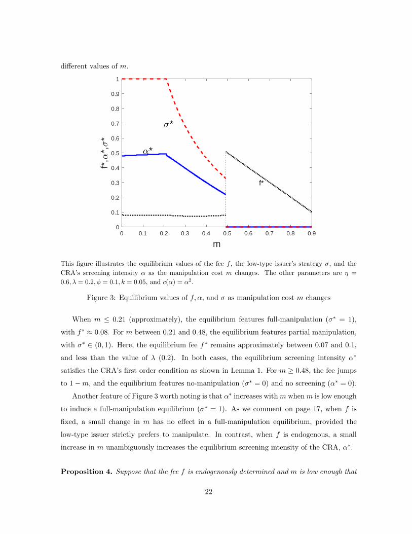
This figure illustrates the equilibrium values of the fee f , the low-type issuer’s strategy σ, and the

CRA’s screening intensity α as the manipulation cost m changes. The other parameters are η =

0.6, λ = 0.2, φ = 0.1, k = 0.05, and c(α) = α2.

Figure 3: Equilibrium values of f, α, and σ as manipulation cost m changes

When m ≤ 0.21 (approximately), the equilibrium features full-manipulation (σ∗ = 1),

with f∗ ≈ 0.08. For m between 0.21 and 0.48, the equilibrium features partial manipulation,

with σ∗ ∈ (0, 1). Here, the equilibrium fee f∗ remains approximately between 0.07 and 0.1,

and less than the value of λ (0.2). In both cases, the equilibrium screening intensity α∗

satisfies the CRA’s first order condition as shown in Lemma 1. For m ≥ 0.48, the fee jumps

to 1−m, and the equilibrium features no-manipulation (σ∗ = 0) and no screening (α∗ = 0).

Another feature of Figure 3 worth noting is that α∗ increases with m when m is low enough

to induce a full-manipulation equilibrium (σ∗ = 1). As we comment on page 17, when f is

fixed, a small change in m has no effect in a full-manipulation equilibrium, provided the

low-type issuer strictly prefers to manipulate. In contrast, when f is endogenous, a small

increase in m unambiguously increases the equilibrium screening intensity of the CRA, α∗.

Proposition 4. Suppose that the fee f is endogenously determined and m is low enough that

22

a full-manipulation equilibrium obtains. Then, dσ∗

dm = 0 and dα∗

dm > 0. That is, the CRA’s

screening intensity increases with m. Further, the price of a high-rated security, p, increases

with m, and the equilibrium rating fee, f∗, decreases with m.

While an increase in m does not affect σ∗ in a full-manipulation equilibrium, it decreases

the issuer’s ex ante payoff. Hence, the bargaining at the initial stage results in a lower

equilibrium rating fee f∗. As a result, the CRA screens more intensely. Finally, the fact

that σ∗ is unchanged whereas α∗ has increased immediately implies that the price of the

high-rated security, p, increases.

This result demonstrates the potential importance of accounting for the effects of changes

in exogenous parameters on the bargaining outcome: With an exogenous rating fee, the

CRA’s strategy does not change with m. It also demonstrates that imposing penalties on

the issuer can, in some circumstances, improve the overall quality of the screening process

and reduce the incidence of ratings errors by lowering the benefit to the CRA of making such

errors.

Our second comparative static result considers changes in η and augments Proposition 3.

Proposition 5. When the fee f is endogenously determined,

(i) In a partial-manipulation equilibrium, dσ∗

dη > 0, dα∗

dη = 0, and dq(α∗,σ∗)dη = dp(α∗,σ∗)

dη = 0,

as in Proposition 3 when f is taken as fixed. In addition, df∗

dη = 0. That is, small

changes in η, the ex ante probability of the high type, have no effect on the equilibrium

fee.

(ii) In a full-manipulation equilibrium, small changes in η lead to a decrease in α∗, an

increase in p, and an increase in f∗.

We illustrate this comparative static in the context of an example. Set λ = 0.2,m =

0.3, φ = 0.1, k = 0.05 and c(α) = α2. As seen in Figure 4, when η < 1√2≈ 0.707, the

equilibrium features partial manipulation by the low-type issuer, with σ∗ ∈ (0, 1). In this

region, σ∗ increases with η, whereas α∗ is flat in η. At first glance, the latter property is

puzzling. As the expected quality of the issuer improves, one may expect that the need for

screening declines. However, the endogenous response of the low-type issuer implies that the

23

average quality of the pool that applies for a rating, in fact, remains constant as η increases

in this range. In contrast, when η > 0.707, the equilibrium features full manipulation, with

σ∗ = 1. In this region, as expected, α∗ decreases with η.

0 0.1 0.2 0.3 0.4 0.5 0.6 0.7 0.8 0.9 10

0.1

0.2

0.3

0.4

0.5

0.6

0.7

0.8

0.9

1f*

,*,

*

f*

*

*

This figure illustrates the equilibrium values of the fee f , the low-type issuer’s strategy σ, and the

CRA’s screening intensity α as η, the prior probability of a high-type issuer, changes. The other

parameters are λ = 0.2,m = 0.3, φ = 0.1, k = 0.05, and c(α) = α2.

Figure 4: Equilibrium values of f, α, and σ as η, the prior probability of a high-type issuer,changes

We illustrate through examples how the rating fee f∗ and equilibrium strategies of the

low-type issuer (σ∗) and the CRA (α∗) vary with the exogenous parameters k, λ, and φ when

the rating fee is determined endogenously. In these examples, we work with the base set of

parameters η = 0.6, λ = 0.2, m = 0.3, φ = 0.1, k = 0.05, and c(α) = α2, unless otherwise

noted. In each example, we vary one of the parameters and plot α∗, σ∗, and f∗ as functions

of that specific parameter. Figure 5 presents plots where we vary first (a) k and then (b) λ.

These figures provide a contrast to the results in Proposition 2. In Figure 5 (a), σ∗

increases in k until k is approximately equal to 0.05, and then flattens out over the range

k ∈ (0.05, 0.065). For k above 0.065, the optimal value of f jumps discretely to 1−m = 0.7. At

24

0 0.01 0.02 0.03 0.04 0.05 0.06 0.07 0.08 0.09 0.1

k

0

0.1

0.2

0.3

0.4

0.5

0.6

0.7

0.8f*

,*,

*

f*

*

*

0.1 0.15 0.2 0.25 0.3 0.35 0.40

0.1

0.2

0.3

0.4

0.5

0.6

0.7

0.8

f*,

*,*

f*

* *

(a) (b)These figures illustrate the equilibrium values of the fee f , the low-type issuer’s strategy σ, and the

CRA’s screening intensity α as k and λ vary. The other parameters are η = 0.6,m = 0.3, φ = 0.1, and

c(α) = α2. For figure (a), λ = 0.2, and for figure (b), k = 0.05

Figure 5: Effect on α∗ and σ∗ as k and λ vary

this point, therefore, σ∗ falls to zero and stays there for higher levels of k. From Proposition

2, if f were held constant, we would expect to see a continuous decrease in σ∗ as k increased

above 0.065.

A similar contrast occurs in Figure 5 (b), when λ varies. For low values of λ (below about

0.16), the optimal value of f is at 1 − m = 0.7, so that we have zero manipulation. As λ

increases above 0.16, f∗ falls discretely to about 0.08. From this point on, σ∗ decreases in λ.

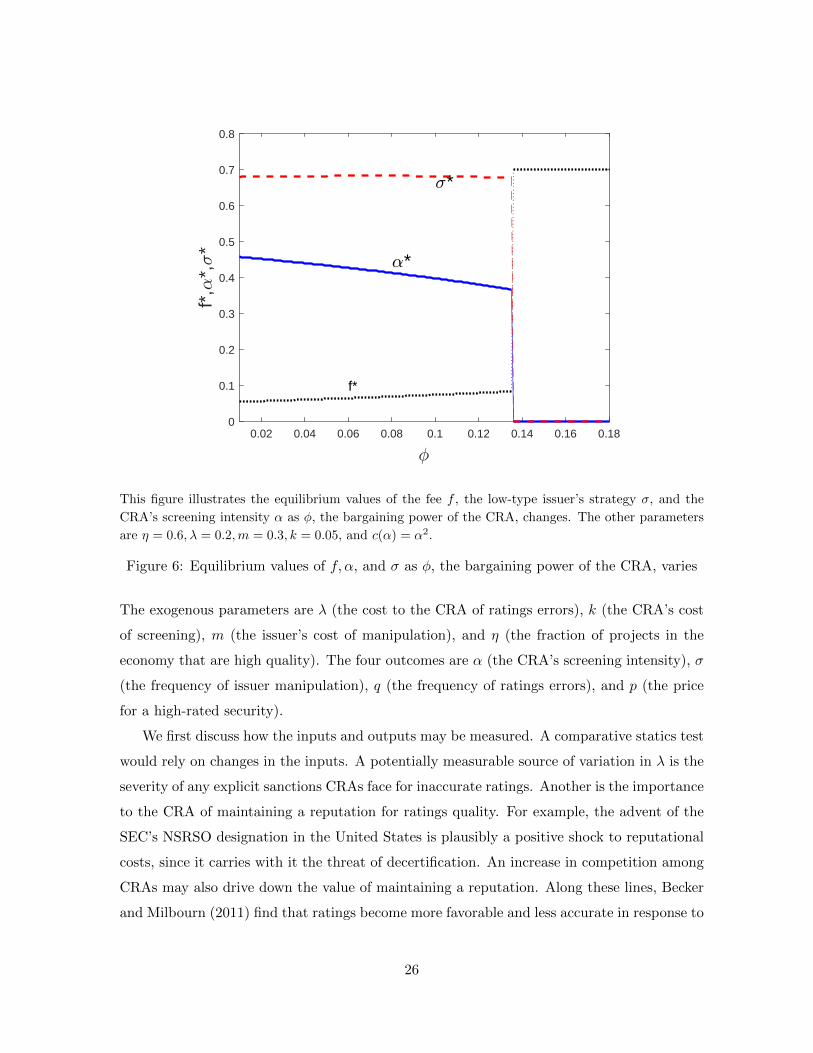
Finally, Figure 6 presents a plot where we vary φ, again setting the other parameter values

to those noted at the beginning of this section. An increase in φ increases the bargaining power

of the CRA, which results in a higher rating fee f∗. As the fee for a high rating increases,

the CRA’s incentives to screen decline, resulting in a lower α∗. Recall that throughout, there

remains a local optimum for f at 1 −m (in the example, 1 −m = 0.7 remains well greater

than the values of φ we consider). At φ approximately equal to 0.135, the equilibrium value

of f jumps discretely to 1−m, with σ∗ and α∗ both equal to zero at this point.

5 Empirical Implications

This section discusses some empirical implications of our model. These implications relate

to the model’s predictions about the effects of four exogenous parameters on four outcomes.

25

0.02 0.04 0.06 0.08 0.1 0.12 0.14 0.16 0.180

0.1

0.2

0.3

0.4

0.5

0.6

0.7

0.8

f*,

*,*

f*

*

*

This figure illustrates the equilibrium values of the fee f , the low-type issuer’s strategy σ, and the

CRA’s screening intensity α as φ, the bargaining power of the CRA, changes. The other parameters

are η = 0.6, λ = 0.2,m = 0.3, k = 0.05, and c(α) = α2.

Figure 6: Equilibrium values of f, α, and σ as φ, the bargaining power of the CRA, varies

The exogenous parameters are λ (the cost to the CRA of ratings errors), k (the CRA’s cost

of screening), m (the issuer’s cost of manipulation), and η (the fraction of projects in the

economy that are high quality). The four outcomes are α (the CRA’s screening intensity), σ

(the frequency of issuer manipulation), q (the frequency of ratings errors), and p (the price

for a high-rated security).

We first discuss how the inputs and outputs may be measured. A comparative statics test

would rely on changes in the inputs. A potentially measurable source of variation in λ is the

severity of any explicit sanctions CRAs face for inaccurate ratings. Another is the importance

to the CRA of maintaining a reputation for ratings quality. For example, the advent of the

SEC’s NSRSO designation in the United States is plausibly a positive shock to reputational

costs, since it carries with it the threat of decertification. An increase in competition among

CRAs may also drive down the value of maintaining a reputation. Along these lines, Becker

and Milbourn (2011) find that ratings become more favorable and less accurate in response to

26

an increase in competition due to the material entry of Fitch as a third major rating agency.

One might imagine capturing information about the direct cost of screening (kc(α))

through measures of the opacity of the assets being rated. All else equal, more opaque

assets are likely to be more difficult to evaluate, necessitating greater CRA effort to screen

out lower-quality assets.

The manipulation cost m varies with at least two factors. First, the cost of manipulation

is likely to be lower for newer securities (such as securities backed by subprime mortgages in

the late 1990s and early 2000s), as the CRA (and the rest of the market) will learn about

the features of a security over time. Second, manipulation is easier (and hence less costly)

when a security is more complex. Expected manipulation costs should also increase with

the ex post legal sanctions for committing fraud, the prosecutorial resources available to the

regulator, and the willingness of courts to convict in fraud cases. For example, the 2002

Sarbanes-Oxley Act can be interpreted as a large positive shock to the cost of manipulating

corporate debt ratings, as manipulation of accounting information is an important means of

influencing CRA beliefs.12

In testing the model’s predictions regarding changes in asset quality, one could imagine

capturing asset quality at a broad level through measures of the state of the economy such as

GDP or the aggregate market-wide Tobin’s Q. One could also imagine measuring asset class-

specific quality through current default rates in the asset class. Note that the model predicts

the absence of a relationship between overall asset quality and both the incidence of ratings

errors and the price of highly-rated securities. This predicted non-relationship represents a

sharp prediction regarding the issuer’s and CRA’s strategic response to an increase in asset

quality, as an improvement in asset quality should mechanically reduce ratings errors and

increase the price of high-rated securities absent these strategic responses.

Turning to the outputs, screening intensity (α in the model) can be measured in several

different ways: by the number of analysts working for a CRA per security rated, the CRA’s

expenses per security rated, and the length and detail of reports accompanying ratings.

Higher σ in the model is naturally interpreted as a greater incidence of issuer manipulation.

Manipulation is unobservable in real time in our model by assumption. However, ex-post

prosecutions or regulatory actions for fraudulent reporting might be a useful indicator of the

12As Begley (2015) shows, some firms even incur real costs (such as reducing R&D expenditures) to reducetheir debt-to-EBITDA ratio in the year before issuing a new security, in an attempt to obtain a more favorablecredit rating.

27

frequency with which such manipulation occurs.

The frequency of ratings errors (q) can be measured directly, at least ex post. For example,

one can compare the default rate of securities in a given class to the stated default rate that

a given rating is supposed to imply. In doing so, it would be useful to filter out the effects of

factors affecting default rates such as the state of the economy that would have been difficult

for a CRA to forecast at the time of the rating.

Finally, the price conditional on a high rating (p) could be measured as the inverse of the

spread on investment-grade securities over the risk-free rate, which could then be compared

across different settings or over time.

We divide our implications into two parts. First, we consider the rating fee f as fixed,

as in Section 3. These implications are relevant for formulating short-run tests of the effects

of factors that affect issuer and CRA behavior, as fees are unlikely to adjust immediately to

small changes in such factors. Next, we consider long-run effects when the fee can adjust as

well, as in Section 4.

5.1 Short-run implications

First, with a fixed fee, our model predicts that CRA screening intensity should rise with

the cost to the CRA of ratings errors, while manipulation frequency should increase in re-

sponse to a cost increase when the cost is low and decrease with a cost increase when the

cost is high (Proposition 2). The first prediction is straightforward and would be common to

most models of CRA screening. However, the second prediction follows from a more nuanced

argument—in considering the issuer’s manipulation decision, the price increase due to greater

screening intensity can more than offset the direct effect of a reduction in the probability that

manipulation succeeds, and it does so in particular when the cost to the CRA of a ratings

error is low. Together, these predictions suggest that when the cost of ratings errors is low,

we should observe both more manipulation and more intense screening in response to an

increase in this cost.

As a practical consideration, testing the model’s prediction of a non-monotone relation-

ship between the frequency of manipulation and the cost of ratings errors would require

observing this cost over a sufficiently large range to encompass the level at which the sign of

the relationship changes. The model makes similar, though opposite, predictions about the

relationships between the four outcomes described above and the cost of screening (k in the

28

model).

Second, the model also makes specific predictions about the variation in strategies and

outcomes with m, the cost of manipulation. However, holding fixed the ratings fee, these

predictions are straightforward and not distinctive features of our model. An increase in

the cost manipulation generally results in less manipulation, to which the CRA responds by

screening less intensely. The net effect is fewer ratings errors and a higher price for high-rated

securities. As we describe next, the model yields more distinct predictions, at least in some

cases, when the ratings fee is endogenously determined through bargaining.

5.2 Long-run implications

First, both in the long- and short-run, our model predicts that the overall incidence of

manipulation does not change over a wide range of asset quality, as captured by the parameter

η. More precisely, in a partial-manipulation equilibrium, the probability that a low-type issuer

manipulates increases enough to perfectly offset the effect of a reduction in the fraction of

low-quality assets on the overall rate of manipulation. The model also predicts that screening

intensity, frequency of ratings errors, and price and quality of high-rated securities do not

change with the underlying quality of assets.

It is surprising that the mix of high- and low-quality projects backing a high-rated security

remains unchanged when the prior belief over asset quality improves. The key is that low-

type issuers manipulate more often as the prior belief improves, in response to the indirect

price improvement effect. This result therefore turns the focus back on issuers in explaining

the mortgage-backed security market in the period before the 2008-09 financial crisis. As

the volume of high-rated MBS increased in the 2000s, one could argue that prior beliefs over

quality were improving. Increased manipulation by the low-type issuer would ensure that

the pool of loans backing a high-rated security in fact was not improving in quality.13 Thus,

there was an increasing gap between the potential and actual quality of MBS securities in

the build-up to the crisis.

Second, with an endogenously determined fee, CRA screening intensity may increase

with the cost of manipulation (m) when that cost starts from a fairly low level (Proposition

4). The novel policy implication here is that imposing penalties on a firm for misreporting

13Note that, with an improvement in the prior quality of loans, lax screening would also imply that additionallow-quality loans would enter this pool.

29

information can improve the effort put in by the CRA as well.

Third, examination of Figure 6 suggests that an increase in CRA bargaining power (φ)

in the issuer-pays model generally leads to less intense CRA screening but has ambiguous

implications for the incidence of manipulation. Specifically, when the CRA has little bar-

gaining power, an increase in that bargaining power causes an increase in the incidence of

manipulation. However, when the CRA already has a strong bargaining position, a further

increase in its bargaining power causes a decrease in the incidence of manipulation. One

could measure φ directly by observing the level of CRA fees and profitability. In addition,

variation in competition among CRAs over time or across markets would also provide a source

of variation in CRA bargaining power vis-a-vis issuers and hence their share of proceeds.

Finally, the analysis in Section 4 yields predictions about the long-run responses of various

outcomes to changes in different parameters that are sharp but may be difficult to test.

Several of the figures in that section show discontinuities in α, σ, and f at threshold parameter

values when f is determined endogenously. While identifying these specific thresholds in the

data would be challenging, a sharp drop in manipulation incidence and screening intensity

accompanied by an increase in rating fee following a small increase in the cost of manipulation

(Figure 3) or cost of screening (Figure 5) would support the model. Similarly, a sharp rise in

manipulation incidence and screening intensity and a fall in the rating fee following a small

increase in the CRA’s cost of ratings errors would also support the model.

6 Conclusion

We argue that strategic disclosure by issuers is an important friction to consider in the

ratings process. Our broad message is that the quality of credit ratings depends on both

the quality of screening and the type and disclosure strategy of the issuer. In our model, an

endogenous increase in CRA screening intensity may be accompanied by either a decrease

or increase in issuer manipulation in response. A decrease in manipulation magnifies the

effect of increased screening intensity on ratings accuracy, while an increase in manipulation

dampens the effect. In addition, the need to account for issuer behavior can undo the effects

of shocks that might otherwise impact the quality of CRA screening.

When assessing periods during which the quality of ratings has been perceived to be

low, it is important to remember that issuers are likely to know more about their own asset

30

qualities than a CRA. Any policy design intended to improve the overall ratings process must

include providing incentives to issuers to truthfully report the quality of their assets as an

important component.

31

Appendix A: Proofs

Proof of Lemma 1. As mentioned in the text, the payoff of the CRA is Ψ = N(σ){νf +

(1 − ν)(1 − α)(f − λ) − kc(α)}

. Holding f fixed, the derivative with respect to α is ∂Ψ∂α =

(1 − ν)(λ − f) − kc′(α). If λ ≥ f , the first-order condition implies that the CRA’s optimal

choice of α satisfies c′(α) = 1−νk (λ − f). As c′′(α) > 0, it follows immediately that the

second-order condition for a maximum is satisfied.

If λ < f , we have ∂Ψ∂α < 0. The optimal choice of α is therefore zero.

Proof of Lemma 2. Suppose the low-type issuer seeks a rating. Seeking a rating and not

manipulating is equivalent to not seeking a rating (since the issuer always gets a low rating,

and is therefore revealed to be a low type). If the issuer seeks a rating and manipulates its

information, it obtains an expected payoff of (1− α)(p− f)−m. If it does not seek a rating,

it does not issue a financial claim and obtains zero. The statement of the lemma follows

immediately.

Proof of Proposition 1. (i) Suppose that m ≤ (1− α1)(p(α1, 1)− f), where α1 is defined

as α1 = c′−1(

1−ηk max{λ− f, 0}

). If the CRA chooses α∗ = α1 and the low-type issuer

chooses σ∗ = 1 (i.e., seeks a rating with probability one), the price of the high-rated asset is

p(α1, 1). From Lemma 2, it follows that if the CRA chooses α∗ = α1, it is a best response

for the low-type issuer to set σ∗ = 1. When σ∗ = 1, ν(σ) = η, so from Lemma 1, it then

follows that it is a best response for the CRA to set α∗ = α1. Thus, there is an equilibrium

in which (α∗, σ∗) = (α1, 1). Further, α1 is a best response only if σ∗ = 1, and σ = 1 is a best

response only if m ≤ (1− α∗)(p(α∗, 1)− f). Therefore, in equilibrium, we can have α∗ = α1

only if m ≤ (1− α1)p(α1, 1)− f .

(ii) Suppose that m ≥ 1− f . If the CRA chooses α∗ = 0 and the low-type issuer chooses

σ∗ = 0, the price of the high-rated security is 1. Now, from Lemma 2, it is a best response

for the low-type issuer to not seek a rating if m ≥ 1 − f . Further, when σ∗ = 0, ν(σ∗) = 1,

so that from Lemma 1, the best response of the CRA is to set α∗ = 0. Therefore, there is

an equilibrium in which (α∗, σ∗) = (0, 0). Further, an equilibrium with α∗ = 0 can exist only

when m ≥ 1− f . At any lower value of m, σ∗ > 0 when α∗ = 0, so that α∗ = 0 cannot be a

best response.

32

(iii) Suppose that m ∈ ((1−α1)(p(α1, 1)−f), 1−f) and consider the conjectured equilib-

rium given by α = c′−1(

1−ν(σ)k max{λ− f, 0}

)and σ = η

1−η

(1−f− m

1−α(1−α)(1+f+ m

1−α )

). The price of

the high-rated security is then p(α, σ) = η−(1−η)σ(1−α)η+(1−η)σ(1−α) . From Lemma 1, it is immediate that

α is a best response to σ. Suppose that the low-type issuer is indifferent between seeking a

rating and not seeking a rating. Then, it must be that (1 − α)(p(α, σ) − f) = m, or that

(1 − α)(η−(1−η)σ(1−α)η+(1−η)σ(1−α) − f

)= m. Solving the last equation for σ yields the value of σ∗ in

the statement of the proposition. It is immediate that σ∗ > 0. Further, σ∗ ≥ 1 implies that

m ≤ (1 − α1)(p(α1, 1) − f . Thus, when m > (1 − α1)(p(α1, 1) − f), we have σ∗ < 1. To

complete the proof, note that given σ∗, the value of α∗ must satisfy the CRA’s first-order

condition.

Proof of Lemma 3. Suppose that f < λ, and let (α∗, σ∗) denote the equilibrium val-

ues in a partial-manipulation equilibrium. Observe that ν(σ∗) =(

1 +(

1−ηη

)σ∗)−1

=(1 +

1−f− m1−α∗

(1−α∗)(1+f)+m

)−1

, where the last equation uses the expression for σ∗ in equation (4).

Substituting this expression for ν(σ∗) into the RHS of equation (5) and re-writing the result-

ing equation, we have that α∗ satisfies the condition h(α∗) = 0, where

h(α) =

(2− α

(1 + f +

m

1− α

))c′(α)− λ− f

k

(1− f − m

1− α

). (12)

Observe that h(0) < 0. Thus, a sufficient condition for uniqueness is that whenever h(α) = 0,

we also have h′(α) > 0. This condition is equivalent to(2− α

(1 + f +

m

1− α

))c′′(α) >

(1 + f +

m

(1− α)2

)c′(α)− λ− f

k

m

(1− α)2. (13)

In a partial-manipulation equilibrium, it must be that α∗ < 1 − m1−f (otherwise σ∗ = 0).

Thus, it follows that 2− α(

1 + f + m1−α

)> 2m

1−f , so a sufficient condition for inequality (13)

to hold is that (2m

1− f

)c′′(α) >

(1 + f +

m

(1− α)2

)c′(α)− λ− f

k

m

(1− α)2. (14)

To obtain condition (6), observe that the equilibrium α∗ satisfies λ−fk = c′(α∗)

1−ν . Hence,

inequality (14) can be written as(

2m1−f

)c′′(α) >

(1 + f − ν

1−νm

(1−α)2

)c′(α). Since ν > η in

33

any partial-manipulation equilibrium and since m(1−α)2

> m, the RHS of this inequality is

therefore strictly less than(

1 + f − ηm1−η

)c′(α). Therefore, inequality (13) is satisfied if

(2m

1− f

)c′′(α) >

(1 + f − ηm

1− η

)c′(α). (15)

This condition is equivalent to the one stated in the lemma.

Proof of Proposition 2. Let y = λ−fk and recall the definition of h(α) from equation (12)

in the proof of Lemma 3. The Implicit Function Theorem implies that dα∗

dy = − ∂h/∂y∂h/∂α .

Further, the second-order condition for α∗ requires that ∂h∂α > 0. By inspection, ∂h

∂y < 0.

Thus, it follows immediately that dα∗

dy > 0, which implies that dα∗

dλ > 0 and dα∗

dk < 0.

Next, let

g(α) =η

1− η

(1− f − m

1−α(1− α)(1 + f) +m

). (16)

From equation (4) in Proposition 1, it follows that in a partial-manipulation equilibrium we

have σ∗ = g(α∗). Further, dσ∗

dy = ∂g∂α

dα∗

dy since ∂g∂y = 0 when y = λ−f

k . From equation (16), we

have

∂g

∂α=

η

1− η

1− f2 − 2m1−α(1 + f)− m2

(1−α)2

[(1− α)(1 + f) +m]2

. (17)

It is immediate to see that ∂g∂α is strictly decreasing in α. Further, ∂g

∂α is strictly negative

at α = 1 − m1−f (the value of α at which σ∗ becomes zero) and strictly positive at α = 0 if

(f +m)2 +2m < 1. Thus, if (f +m)2 +2m < 1, there exists a threshold α ∈ (0, 1− m1−f ) such

that dσ∗

dy > 0 for α < α and dσ∗

dy < 0 for α > α. Since α∗ increases in y and since y decreases

in k, this implies that there exists a k such that dσ∗

dk > 0 for k < k and dσ∗

dk < 0 for k > k.

Similarly, since y increases in λ, there exists a λ such that dσ∗

dλ > 0 for λ < λ and dσ∗

dλ < 0 for

λ > λ.

Proof of Proposition 3. Consider the function h(α), as defined in equation (12) in the

proof of Lemma 3. Recall that a partial-manipulation equilibrium is defined by h(α∗) = 0.

Thus, for any x ∈ {η, k, λ,m, f}, from the Implicit Function Theorem we have dα∗

dx = − ∂h/∂x∂h/∂α .

By inspection, ∂h∂η = 0, so it follows that dα∗

dη = 0.

34

To calculate dσ∗

dη , recall from equation (4) in Proposition 1 that

σ∗ =η

1− η

(1− f − m

1−α∗

(1− α∗)(1 + f) +m

). (18)

It follows that, for any x ∈ {η, k, λ,m, f}, we have dσ∗

dx = ∂σ∗

∂x + ∂σ∗

∂α∗dα∗

dx . As dα∗

dη = 0 and (by

inspection) ∂σ∗

∂η > 0, it is immediate that dσ∗

dη > 0.

Finally, note that in a partial-manipulation equilibrium, it must be that (1−α∗)(p−f) =

m. For small changes in the exogenous parameters, the equilibrium continues to feature

partial manipulation, so this equation must continue to hold. As α∗ is invariant to η, it

follows that p must also remain constant for small changes in η.

Proof of Lemma 4. (a) Consider values of f close to but strictly less than 1 −m. From

Proposition 1, for some f1 < 1 − m, whenever f > f1 we have σ∗ ∈ (0, 1). Then, the

indifference condition of the low-type issuer implies that p−f = m, or f = p−m. Observe that

when α∗ = 0, we can write the ex ante payoff of the issuer as Π = η(p−f)+(1−η)σ(p−f−m) =

η(p− f) = ηm when σ ∈ (0, 1). Thus, over the region (f1, 1−m], Π is invariant to f .

Now, the payoff of the CRA may be written as Ψ =(η + (1− η)σ

)(p−m)− (1− η)σλ.

When α∗ = 0, we have p = η−(1−η)ση+(1−η)σ . Thus, Ψ = η(1 −m) − (1 − η)σ(1 + λ −m). When

λ < 1 −m, it follows that m < 1 + λ. Therefore, Ψ is strictly decreasing in σ, and hence is

maximized at σ = 0. When α∗ = 0, to induce σ = 0, it must be that f = 1−m. Hence, over

the region [f1, 1−m], the Nash product H(f) is maximized at f = 1−m.

Now, consider values of f > 1 −m. At these values, from Proposition 1, we have σ = 0

and α = 0. Therefore, for f in this region, we have Ψ = ηf , and Π = η(1 − f). From the

Nash maximization problem, it now follows that the optimal value of f is max{φ, 1−m}.

Hence, the Nash product has a local optimum at f = max{φ, 1−m}.

(b) For f close to zero, it follows that Ψ < 0, so the Nash product is undefined. At f = λ,

we have α∗ = 0, so that Ψ(f) > 0. It is immediate that there must be a minimal level of f ,

which we denote f , such that Ψ ≥ 0 if and only if f ≥ f . Therefore, a sufficient condition to

ensure that H(·) has an interior maximum on (0, λ) is that limf→λ− H′(f) < 0.

35

Now, observe that

H ′(f) = (1− φ)

[Ψ(f)

Π(f)

]φΠ′(f) + φ

[Π(f)

Ψ(f)

]1−φΨ′(f) (19)

Thus, when Ψ > 0 and Φ > 0, the condition H ′(f) < 0 is equivalent to

(1− φ)Π′(f)

Π(f)+ φ

Ψ′(f)

Ψ(f)> 0. (20)

Now, consider the CRA’s expected payoff Ψ, shown in equation (8), as f → λ−. When

α∗ > 0 (which will obtain as long as f < λ and σ∗ > 0), using the CRA’s first-order condition

kc′(α) = (1− ν)(λ− f) and the definition of ν(σ∗), we can write

Ψ(f) = ηf − kN(σ∗)[(1− α∗)c′(α∗) + c(α∗)] (21)

Thus, Ψ′(f) = η − k{N(σ∗)(1− α∗)c′′(α∗)dαdf −N

′(σ∗)[(1− α)c′(α∗) + c(α∗)]}

dα∗

df . Now,

differentiating the CRA’s first-order condition, we have kc′′(α)dαdf = −(1 − ν(σ∗)) − (λ −

f)ν ′(σ∗)dσdf .

Now, when f → λ−, in the limit α∗ = 0. Further, let σλ denote denote the equilibrium

value of σ∗ in the screening game when f = λ. Making the relevant substitution and taking

the limit as f → λ−, we obtain

limf→λ−

Ψ′(f) = η + (1− η)σλ = N(σλ), (22)

Finally, note that limf→λ− Ψ(f) = ηλ. Therefore, limf→λ−Ψ′(f)Ψ(f) = λ

ν(σλ) .

For the term Π′(f)Π(f) in condition (20), there are two cases to consider. First, suppose that

λ+m > 2η−1. Then, from equation (4) in Proposition 1, it follows that σλ = η1−η

1−λ−m1+λ+m < 1.

Now, observe that σ∗ < 1 implies that (1 − α∗)(p(α∗, σ∗) − f) = m (else the low type is

not indifferent between manipulating and not). Therefore, whenever σ∗ < 1, the expected

surplus of the issuer is Π(f) = N(σ)∗ν(σ∗)(p − f) = ηm1−α∗ . Hence, Π′(f) = ηm

(1−α∗)2dα∗

df .

Further, totally differentiating the CRA’s first-order condition,

dα∗

df= −

[1− ν(σ∗)] + ν ′(σ∗)(λ− f)dσ∗

df

kc′′(α∗)(23)

36

Putting all this together, in the limit as f → λ−, we obtain:

limf→λ−

Π′(f) = −ηm1− ν(σλ)

kc′′(0). (24)

Further, limf→λ− Π(f) = ηm, so that limf→λ−Π′(f)Π(f) = −1−ν(σλ)

kc′′(0) .

Making all the appropriate substitutions, when λ+m > 2η−1 we have limf→λ− H′(f) < 0

if and only if −(1− φ)1−ν(σλ)kc′′(0) + φ 1

ν(σλ)λ < 0, or

φ <λν(σλ)[1− ν(σλ)]

λν(σλ)[1− ν(σλ)] + kc′′(0)(25)

Now, from σλ = η1−η

1−(λ+m)1+(λ+m) , it follows that ν(σλ) = 1+m+λ

2 and so ν(σλ)(1 − ν(σλ)) =1−(m+λ)2

4 . Substituting this expression into (25) and simplifying gives the following condition

for limf→λ− H′(f) < 0:

φ <λ[1− (m+ λ)2]

λ[1− (m+ λ)]2 + 4kc′′(0). (26)

Denote the right-hand side as φ1.

Next, suppose that m + λ ≤ 2η − 1, so that σλ = 1. In this case, we can write Π(f) =

R(α∗)(p − f) − (1 − η)m, where R(α∗) = n + (1 − η)(1 − α∗) is the proportion of issuers

who succeed on obtaining a high rating. Thus, Π′(f) = ( ∂p∂αdα∗

df − 1)R − (1 − η)(p − f)dα∗

df .

Now, observe that p = 2η−RR = 2η

R − 1. Thus, ∂p∂α = 2η(1−η)

R2 . Therefore, we have Π′(f) =

−R+(1−η)(1+f)dα∗

df . When σ∗ = 1, differentiation of the CRA’s first-order condition yields

dα∗

df = − 1−ηkc′′(α∗) . Making the relevant substitutions, and recognizing that α∗ → 0 and p →

2η − 1 as f → λ−, we obtain limf→λ−Π′(f)Π(f) = −

1+(1−η)2(1+λ)

kc′′(0)2η−1−λ−(1−η)m . Denote Z =

1+(1−η)2(1+λ)

kc′′(0)2η−1−λ−(1−η)m .

Recalling that λ+m ≤ 2η − 1, it follows that Z > 0.

Now, the condition for H ′(f) < 0 is equivalent to −(1−φ)Z+φλη > 0, or φ < ZZ+λ

η

d= φ2.

Define φ = φ1 if λ+m > 2η− 1 and φ = φ2 otherwise. Then, it follows that when φ < φ,

the Nash product H(f) has an interior optimum on (0, λ). It follows immediately that the

first-order condition H ′(f) = 0, or φΠ′(f)Π(f) = −(1− φ)Ψ′(f)

Ψ(f) , is satisfied at this optimum.

Proof of Proposition 4. Suppose we are in a full-manipulation equilibrium, so that σ∗ = 1.

Recall that ν(1) = η. Consider a small increase in m. For a sufficiently small change, it

continues to be the case that σ∗ = 1 in the new equilibrium. However, keeping α fixed, the

37

expected surplus of the issuer falls, as the payoff of the low type decreases in m. Therefore, f∗

must fall. Further, the first-order condition of the CRA, given by kc′(α∗) = (1− η)(λ− f∗),

implies that as f∗ falls, α∗ increases. As α∗ increases, and σ∗ remains at 1, it is immediate

that the price p must increase.

Proof of Proposition 5. (i) As in the case with a fixed rating fee f , the screening intensity

α∗ in a partial-manipulation equilibrium has to satisfy the condition h(α∗) = 0, where h(α)

is defined in equation (12) (with f = f∗). In addition, α∗ and f∗ have to satisfy the equation

φΠdΨdf = −(1− φ)ΨdΠ

df . Note that h(α) does not depend on η; further, f∗ depends on η only

through ν(σ∗). Recall from the proof of Lemma 3 that in a partial-manipulation equilibrium

ν(σ∗) can be expressed as ν(σ∗) =(

1 +1−f− m

1−α∗(1−α∗)(1+f)+m

)−1

. This means that the effect of a

(small) increase in η on ν is offset by an increase in σ∗, leaving ν unchanged. Of course, if ν

is unchanged, so are α∗, f∗, and p(α∗, σ∗).

(ii) Consider a full-manipulation equilibrium. Since m is increasing in η, an increase in η

means that we continue to have σ∗ = 1. The equilibrium screening intensity satisfies kc′(α∗) =

(1 − η)(λ − f∗). As η increases, keeping σ∗ fixed at 1, ν increases. Therefore, α∗ decreases.

Nevertheless, the increase in η implies that p increases, and in turn f∗ increases.

38

Appendix B: Additional Comparative Statics with Fixed f

In this section, we consider the comparative statics of α∗ and σ∗ for the case in which the

rating fee f is fixed, as the manipulation cost m and rating fee f vary. Suppose throughout

that we have a partial-manipulation equilibrium, and suppose further that f < λ.

First, consider changes in f . Following the technique used in the proof of Proposition 2,

observe that when y = λ−fk , it is immediate that dy

dk < 0. As dα∗

dy > 0 in a partial-manipulation

equilibrium, it follows that dα∗

df < 0.

Now, as in the proof of Proposition 2, we have dσ∗

df = ∂g∂f + ∂g

∂αdα∗

df , where g(α) =

η1−η

(1−f− m

1−α(1−α)(1+f+ m

1−α)

). It is immediate that ∂g

∂f < 0. Thus, if ∂g∂α > 0 (i.e., when (f +m)2 +

2m < 1 and α is small), it follows that dσ∗

df < 0. However, if α is large or (f +m)2 + 2m > 1,

then ∂g∂α < 0, so it is not immediate to determine the sign of dσ∗

df .

Next, consider changes in m, the manipulation cost for the low-type issuer. We have

∂h∂m =

−αc′(α)+λ−fk

1−α . Recalling that α∗ is defined by the equation c′(α∗) = λ−fk (1−ν(σ∗(α∗))),

we have ∂h∂m = λ−f

k(1−α)(−α(1 − ν) + 1) = λ−fk(1−α)(1 − α + να) > 0. As ∂h

∂α > 0, it follows that

dα∗

dm = −∂h/∂m∂h/∂α < 0.

Now, observe that α∗ and σ∗ must satisfy the equation c′(α∗) = λ−fk (1−ν(σ∗)). Consider

a small increase in m. As α∗ decreases, so does c′(α∗). Therefore, it must be that ν(σ∗)

increases, which in turn implies that σ∗ decreases. Therefore, dσ∗

dm < 0.

39

References

Becker, B., and T. Milbourn, 2011, “How did increased competition affect credit ratings?,”

Journal of Financial Economics, 101(3), 493–514.

Begley, T., 2015, “The Real Costs of Corporate Credit Ratings,” Working Paper, SSRN.

Bolton, P., X. Freixas, and J. Shapiro, 2012, “The Credit Ratings Game,” Journal of Finance,

67, 85–112.

Bouvard, M., and R. Levy, 2017, “Two-Sided Reputation in Certification Markets,” Man-

agement Science, forthcoming.

Cohn, J. B., and U. Rajan, 2013, “Optimal Corporate Governance in the Presence of an

Activist Investor,” Review of Financial Studies, 26(4), 985–1020.

Deng, M., N. Melumad, and T. Shibano, 2012, “Auditors Liability, Investments, and Capital

Markets: A Potential Unintended Consequence of the Sarbanes-Oxley Act,” Journal of

Accounting Research, 50(5), 1179–1215.

Department of Justice, 2015, “Justice Department and State Partners Secure $1.375 Bil-

lion Settlement with S&P for Defrauding Investors in the Lead Up to the Financial Cri-

sis,” https://www.justice.gov/opa/pr/justice-department-and-state-partners-secure-1375-

billion-settlement-sp-defrauding-investors.

Frenkel, S., 2015, “Repeated Interaction and Rating Inflation: A Model of Double Reputa-

tion,” American Economic Journal: Microeconomics, 7, 250–280.

Fulghieri, P., G. Strobl, and H. Xia, 2014, “The Economics of Solicited and Unsolicited Credit

Ratings,” Review of Financial Studies, 27, 484–518.

Gill, D., and D. Srgoi, 2012, “The optimal choice of pre-launch reviewer,” Journal of Eco-

nomic Theory, 147(3), 1247–1260.

Goel, A. M., and A. V. Thakor, 2015, “Information reliability and welfare: A theory of coarse

credit ratings,” Journal of Financial Economics, 115(3), 541–557.

Hillegeist, S. A., 1999, “Financial reporting and auditing under alternative damage appor-

tionment rules,” The Accounting Review, 74(3), 347–369.

40

Laux, V., and P. Newman, 2010, “Auditor liability and client acceptance decisions,” The

Accounting Review, 85(1), 261–285.

Mathis, J., J. McAndrews, and J.-C. Rochet, 2009, “Rating the Raters: Are Reputation Con-

cerns Powerful Enough to Discipline Rating Agencies?,” Journal of Monetary Economics,

56(1), 657–674.

Nagy, T., 2009, “Credit Rating Agencies and the First Amendment: Applying Constitutional

Journalistic Protections to Subprime Mortgage Litigation,” Minn. L. Rev., 94, 140.

Sangiorgi, F., and C. Spatt, 2017, “Opacity, Credit Rating Shopping, and Bias,” Management

Science, 63(12), 4016–4036.

Skreta, V., and L. Veldkamp, 2009, “Ratings Shopping and Asset Complexity: A Theory of

Ratings Inflation,” Journal of Monetary Economics, 56(5), 678–695.

Strobl, G., 2013, “Earnings Manipulation and the Cost of Capital,” Journal of Accounting

Research, 51(2), 449–473.

Tsebelis, G., 1990, “Penalty has no impact on crime: A game-theoretic analysis,” Rationality

and Society, 2(3), 255–286.

41