
Credit Exposure and Valuation of Revolving Credit Lines · 2010-11-19 · Credit Exposure and...
32
Credit Exposure and Valuation of Revolving Credit Lines Robert A Jones * Yan Wendy Wu † 19 July 2009 Preliminary * Corresponding author. Department of Economics, Simon Fraser University, Burnaby, BC, V5A 1S6 Email: [email protected] † School of Business & Economics, Wilfrid Laurier University, Waterloo, Ontario, N2L 3C5. Phone: 519-884-0710 ext. 2925. Fax: 519-888-1015. E-mail: [email protected]. 1
Transcript of Credit Exposure and Valuation of Revolving Credit Lines · 2010-11-19 · Credit Exposure and...

Credit Exposure and Valuation of Revolving Credit Lines
Robert A Jones∗ Yan Wendy Wu†
19 July 2009
Preliminary
∗Corresponding author. Department of Economics, Simon Fraser University, Burnaby, BC, V5A 1S6 Email: [email protected]†School of Business & Economics, Wilfrid Laurier University, Waterloo, Ontario, N2L 3C5. Phone: 519-884-0710 ext.
2925. Fax: 519-888-1015. E-mail: [email protected].
1

The revolving credit line—an arrangement under which customers may borrow and repay at will
subject to a maximum outstanding—is the dominant form of bank commercial lending. The interest rate
paid on borrowings, or the spread over some reference rate in the case of floating rate loans, is typically
fixed for the term of the contract. This grants a valuable option to the borrower: As credit quality, and
hence rate that would be paid on alternative borrowings, subsequently fluctuates, he can raise or lower
borrowings on the line. The loan spread, likelihood of default, and line utilization from the perspective of
initial credit quality may thus present a misleading picture of both loan profitability and life-of-contract
credit exposure.
This paper examines credit lines using the tools of contingent claims analysis. It provides a broadly
applicable, computationally tractable, arbitrage-free framework for defaultable securities when creditwor-
thiness evolves independently of the security being valued. I.e., the security in question does not itself
influence solvency of the issuer.
In the terminology of Duffie and Singleton (1997), we use a reduced-form rather than structural model.
Credit quality is assumed to be a one-dimensional latent factor following a mixed jump-diffusion process.
Parameters of the credit quality process can be chosen to represent a wide range of default models,
including ratings transition, pure diffusion to barrier and Poisson jump to default. Model parameters are
estimated by fitting to a limited set of US bond prices. These estimates form the basis for a range of
numerical experiments on hypothetical credit lines. Readily computable are forward looking properties
of the line of concern to lenders such as current fair market value (profitability), probability of default,
expected default losses and sensitivity of market value to fluctuations in credit quality. Further, the role
of contract features such as facility and origination fees, loan term and linking of loan spread to credit
quality (borrower CDS rates) are examined.
Borrower behaviour is characterized as quasi-rational. It can range from sharp-pencilled, fully rational
option exercise, for borrowers with liquid alternative capital market funding sources, to those with non-
existent alternatives, or loan utilization dictated by business considerations outside the model.
We introduce a novel measure of credit exposure to render results meaningful to credit managers
and regulators: Exposure under a revolving credit line can be expressed in terms of its bond equivalent.
This is the principal amount of a constant balance floating rate loan, of same term as the credit line,
which would have the same upfront cost of protection via credit default swap (CDS) as would a custom
CDS compensating the bank for default losses under the line. Essentially, this constant balance loan and
2

the revolving credit line have the same expected present value of default losses under the risk-neutral
valuation measure. For example, a 100mm 3 year credit facility, of which 20mm is intially drawn and with
expected utilization rate of 40% over its life, might be characterized as having credit exposure equivalent
to a 75mm fixed term loan. Such metrics are clearly relevant to both bank management and to regulators
incorporating loan committments into capital adequacy requirements.
Several features of credit lines become apparent. First, credit line value depends critically on borrower
drawdown behaviour. Higher loan spreads are required for a lender to break even with borrowers who
adjust drawdown and repayment according to their cost of borrowing elsewhere. Second, for borrowers
with line utilization highly sensitive to alternative borrowing costs, there may not exist any finite spread
sufficient for the lender to break even. Hence other fees such as originatin fees, facility fees, standby
fees, or a combination of them are necessary. Third, value to the lender does not necessarily increase
monotonically with loan spread. Higher spreads may decrease utilization enough to reduce loan value.
Last, we find that the presence or absence of the jump component in credit quality dramatically influences
bond equivalent credit exposure. Ignoring potential for jumps can lead to overvaluation of credit lines
and understatement of risk.
Valuation and measurement of risk exposure of credit lines is relevant to both bank management and
regulators incorporating loan commitments into capital adequacy requirements. The findings of this paper
should prove useful to banks with a large proportion of loans in this format. The model provides a tool for
banks to assess pricing policies and to evaluate credit exposure of RCLs for purpose of designing effective
risk management strategies. Regulators might benefit from the framework to gain better understanding of
the risk profile of RCLs and appropriate capital ratios. Current Bank for International Settlements (BIS)
rules measures loan exposure for a commercial credit line as the currently drawn amount plus 50 percent
of the undrawn amount (0 if original maturity 1 year or less). Such uniform treatment for RCLs does
not accurately reflect their risk. Our model provides a more rigorous framework for its computation.1
The paper is organized as follows: Section 1 presents the model of credit quality evolution and
default. As is, it is applicable not only revolving to revolvers but also to bonds, credit default swaps,
CDS swaptions and other credit derivatives that might be written on a firm or used to hedge credit
exposure to it. Section 2 describes the credit line contract, assumptions regarding borrower behaviour,
and numerical solution for its value. Section 3 presents the various numerical experiments. Section 4
discusses background and related literature. Section 5 concludes.1Basel II regulations being phased in are somewhat more complex.
3

I. The default process and security valuation
1. Credit quality evolution
Any operational framework for analyzing the full range of default and credit contingent claims should
recognize certain empirical realities: (i) credit spreads on firm debt2 are positive even at short maturities,
(ii) credit spreads vary with term, (iii) credit spreads fluctuate over time, (iv) default can occur either
without warning (jump) or be seen to be coming, (v) credit spreads can jump without default occuring.
With this in mind, let us treat credit quality as a scalar s(t) that follows a calendar time independent
jump-diffusion process. As a Markov process, this provides computational tractability, facilitates treat-
ment of securities with American option features, and allows room for a second factor that may influence
contractual payouts or values (e.g., riskfree interest rates, variable entering swap or option contract,
credit quality of counterparty, etc.). Default is associated with the credit state crossing an exogenously
specified barrier, here s = 0. Thus
ds = αdt+ σ dz + µdπ (1)
in which z(t) is a standard Brownian motion, π(t) counts the jumps in a Poisson process with instanta-
neous intensity λ, independent of z, α is the diffusion drift, σ the diffusion volatility, and µ the (random)
jump size conditional upon a jump occurring. α, σ, λ are permitted to be ‘nice’ functions of s. Jump
sizes are specified by a conditional distribution function
F (x, x′) ≡ prob{s(t+) ≤ x | s(t−) = x′, dπ(t) = 1} (2)
with µ otherwise independent of z and π.3 That is, F is the cumulative probability distribution function
for credit quality s immediately after a jump. The resulting default time—first t such that s(t) ≤ 0—will
be denoted by τ . Default states are treated as absorbing: i.e., ds(t) = 0 for t > τ .
2. Theoretical security values
Assume there is a continuously functioning, frictionless market in default-free bonds. Let r(t) denote the
interest rate on instantaneously maturing bonds at time t, with the process for r being independent of s.2Difference between par coupon rate and default-free rates of same maturity3Appropriate choice of the functions α, σ, λ, F allows representation of a wide range of reduced-form default models,
such as ratings-based specifications (α, σ = 0, F a step function), pure diffusion to barrier (λ = 0), jumps are always to
default (F (x, x′) steps up from 0 to 1 at x = 0 ∀x′), fixed distribution of jump sizes (F (x+ y, x′ + y) = F (x, x′) ∀x, x′, y),
and so on.
4

Consider financial securities—or contracts between two parties—of the following form: There is a
finite set {ti}i=0,1,... of contractual payment dates. Contract maturity T is the last payment date; contract
origination t0 = 0 is the first. One party is designated the purchaser or lender, and treated as default free;
the other, the seller or borrower, has credit quality evolve as in the previous section. Security valuation
is from the perspective of the lender.
The contract specifies net payments to the lender on payment dates of q(s, r, ti) if no prior default,
where s, r are values at ti. At each t there is also a contractual recovery balance B(s, r, t). If default
occurs at time τ , the lender receives ρB(s, r, τ) at that time. ρ is a recovery rate assumed constant in
the current application.4 Initial loan advance, origination fees or purchase price are subsumed in the
(possibly negative) origination date payment q(s, r, 0).5
Consistent with equilibrium in the absence of arbitrage opportunities, we assume existence of a (risk-
neutral) probability measure Q over realizations such that the time t fair market value of the contract,
conditional on no prior default, is the expected discounted cash flows remaining:
V (s′, r′, t) = EQ[∑
t≤ti<τR(ti)q(s, r, ti) + iτ<TR(τ)ρB(s, r, τ) | s(t) = s′, r(t) = r′, τ > t ] (3)
where iτ<T is an indicator taking value 1 if τ < T , otherwise 0, and
R(ti) ≡ e−∫ ti
t r(x)dx (4)
is the riskless rate discount factor along the realized path.
We treat r as deterministic for the experiments of the current paper. Discount factors R(ti) can thus
be calculated directly and consideration of the r state will be suppressed. Numerical solution for V (s, r, t)
is obtained by recursively working back from contract maturity T in a discretized state space. Details of
the procedure are provided in Appendix A.4Though B will be interpreted in what follows as the contractual loan balance, it could readily be the netted fair market
value of a portfolio of derivatives in which the ‘borrower’ is the counterparty, payment received under a credit default swap
based on the borrower, etc. Depending on the application, the s referred to might be s(τ+), embodying say a dependence
of recoveries on how far s jumped into a default region, or it might be s(τ−), embodying the influence of prior credit state
on borrower actions such as drawdowns on a credit line.5Contractual payments q and recovery balance B will generally depend on actions taken by borrower or lender that are
permissible under the contract—e.g., drawdown of a credit line or exercise of an option. These plausibly depend on the
entire time path of r, s up to the date of such action(s). The current specification assumes that actions influencing contract
payments and recovery balance at time t are functions of the then current s, r only, that the contingent actions of both
parties are known to the lender, and that all this is already incorporated in functions q,B. That said, some dependence of
contractual payments on prior dates’ states will be accomodated, reflecting for example the payment of interest in arrears
on loans or swaps.
5

3. Process specification
After some experimentation with fit to bond price data (see below), and desiring to keep the number of
parameters small, the following specification was adopted for the processes involved:
α(s) = κ(s̄− s)
σ(s) = σ
λ(s) = λ0 max{0 , e(10−s)δ − 1
e10δ − 1}
F (s, s′) =
0 s < a
(s− a)/(b− a) s∈ [a, b]
1 s > b
That is, the diffusion volatility of credit quality s is constant; the diffusion drift is mean-reverting; the
instantaneous jump intensity is an exponential function with maximum value λ0 at the default boundary,
declining to 0 for s at 10 or above, with curvature parameter δ; and s-levels after a jump are uniformly
distributed over a fixed interval [a, b].6
For this specification there are thus eight time-invariant model parameters, including the recovery
rate in default: θ ≡ {κ, s̄, σ, λ0, δ, a, b, ρ}.
4. Parameter estimation
We obtain estimates of the model parameters from US corporate bond prices. The data set available to
us consisted of month-end bond price quotes, obtained from Interactive Data Corporation, for 737 US
firms with publicly traded debt. Prices were available for the period May 1993 to December 1997. Even
within this period, observations were missing much of the time for a majority of firms. Prices for two
months, May 1996 and January 1997, were missing for all bonds. Altogether there were 114614 price
observations.
From this, a subset of 105 firms was selected which (i) had price observations every month (except for
May 96 and Jan 97 as noted above), and (ii) had multiple bond issues outstanding during the period.7
6The choice of 10 as the instantaneously default-free credit quality can be viewed as just a scaling parameter given the
rest of the specification. Regarding F , experiments were conducted with uniform and normally distributed relative and
absolute jumps. λ(s) approaches linear as δ → 0 .7Since the default model gives an exact fit to any single market price quote on a given day by construction, firms with
single debt issues were excluded as not legitimately testing the model.
6

Only non-callable, fixed rate bonds were considered. This left 40,955 price observations. The included
bonds had agency credit ratings ranging from B to AAA, and maturities ranging from a few months to
over 25 years. Average number of bonds outstanding per firm at month end was 8.
Although this subset has many thousands of price observations, certain of its aspects qualify any infer-
ence drawn. First, 1993-97 was a period of continuous economic growth. It misses the recessions of 1991,
2001 and 2008 and consequent evidence on the behavior of corporate bond prices in such circumstances.
Closely related is the fact that no firms in the sample actually defaulted during this time period. Second,
the data set ends before the dramatic mid-1998 rise in credit spreads, which has been characterized by
some observers as more a drying-up of liquidity than a widespread deterioration in credit quality. Such
phenomena are of obvious importance for both portfolio and single-issuer analysis, and inclusion of such
periods could quantitatively affect conclusions.
Estimation was exclusively of the risk-neutral process parameters. I.e., those which, when used to gen-
erate a probability measure Q over realizations, make equation (3) a predictor of observed market prices.
These are the parameters investors behave as if they believed in, were they actually risk-neutral; they
typically differ from those describing the objective process of s over time, since investors are risk-averse
and not all risks are diversifiable. Additionally, our abstract credit quality is not explicitly observable
and must itself be inferred from observed bond prices.
The estimation procedure and resulting parameter estimates are described in Appendix B. These
parameters give quite a good fit to the observed bond prices. Standard deviation of the price residuals
is .70 (on par value of 100). Expressed as yield to maturity residuals, 53% of observations are below 5
basis points, 77% are below 10 bp, 95% are below 25 bp, 99% are below 50 bp.
II. Revolving credit line
1. The loan contract
The loan contract grants the borrower for a fixed term the right—if no default to date—to borrow and
repay at will up to fixed amount. We further specialize this as follows: There is a fixed payment interval
associated with the loan (e.g., monthly) during which interest accrues. Drawdowns and repayments can
only occur on these ‘payment dates’. Default, though it may be reached between such dates, will only
be recognized as of these dates.
7
Interest accrues between payment dates at a fixed spread above the level of a default-free reference
rate rref as of the beginning of the interval.8 The reference rate is the then prevailing market rate (simple
interest) on a default-free zero-coupon instrument of term reference rate maturity (e.g., 90 day Libor
rate). Additionally, the balance due may accrue a facility fee payable on the full credit line amount,
and/or a standby fee payable on the amount undrawn during the interval. The latter are expressed as
(simple) interest rates per year. Finally, an up-front origination fee expressed as percent of maximum
loan amount, may be charged.9
Contract parameters are thus: the fixed term T , maximum loan amountA, set of repayment/drawdown
dates {ti}, reference rate maturity Tref, loan spread c, facility cf , standby cs and origination co fees. These
parameters, together with drawdowns and the reference rate at the beginning of a payment interval, de-
termine a contractual balance owed at the end of an interval. This is the basis for recoveries if default
occurs within the interval; this is the amount assumed paid in full if default does not occur, to be then
followed by a new drawdown.10
A relatively recent development in credit line contracts is grid-pricing, the linking of loan spread to
either the agency credit rating or the credit default swap spread of the borrower. We incorporate one
variant of the latter. The contractual rate at which loan interest accrues is assumed to take the form
rcon = rref + c+ βmax{0, ropp − rref − c} (5)
I.e., if the borrower’s current CDS spread ropp − rref exceeds the base loan spread, then a proportion
β of that excess is added to the current period loan rate. Note that although β would typically be
between 0 and 1, setting it to infinity could be used to effectively suspend the credit line whenever CDS
spread exceeds c. The role of such provision is to reduce the moral hazard associated with the borrower’s
drawdown option.
2. Borrower drawdown behaviour
There is little empirical evidence regarding drawdown behaviour on credit lines. Kaplan and Zingales
(1997) find that the undrawn portion of credit lines decreases when firms are more liquidity constrained.8Fixed rate rather than fixed spread credit lines, typical for most credit cards, can be easily accomodated but are not
done so here.9Since any given standby fee and be re-expressed as an equivalent change in the facility fee and spread, it will be
suppressed in the remaining sections of the paper.10Realistically, of course, these two transactions occur simultaneously and show up as just a net change in drawdowns.
8
Gatev and Strahan (2006) report that drawdowns increase when the commercial paper–Tbill rate spread
rises. Both studies suggest interest incentives at work. This motivates the following.
Let ropp denote the fair rate (i.e., opportunity cost) at which the borrower could currently issue
commercial paper for term of one payment interval, given his then-current credit quality. We assume
that the proportion of the credit line drawn is an increasing function f(g) of the difference, g ≡ ropp−rcon,
between this alternative opportunity rate and the marginal cost of line borrowings. This means that when
the contractual interest rate is not fully adjusted to reflect the deterioration of a borrower’s credit quality,
i.e. β < 1, the closer is the borrower to default, the higher his utilization of the line. Moral selection—in
the sense that line utilization is higher when credit quality is lower—is present.
Were borrower behaviour completely rational, he should use nothing from the credit line when g is
negative, and draw the maximum g is positive. But in practice, firms seldom use credit lines this way. We
wish to account for the fact that borrower behavior may be rational to varying degrees—or influenced by
factors other than just immediate borrowing costs—by specifying a flexible functional form that includes
full ‘rationality’ as a special case. Hence, we assume the drawdowns take the following form:
f(g) = dmin + (dmax − dmin)N(dsen g) (6)
Here N( ) is the standard normal distribution function, which varies between 0 and 1. Behavioural
parameters dmin, dmax and dsen represent respectively minimum and maximum drawdowns and sensitivity
to g. The amount borrowed for interval [ti, ti+1] is thus Af(gti). Fully rational behavior in this model
is characterized by dsen = ∞. Constant borrowing is characterized by dsen = 0. Although this is
a deterministic relationship, note that for valuation purposes we may also interpret f(g) as expected
drawdown, with the expectation taken over operational and cash-flow factors excluded in model as long
as such factors are statistically independent of credit quality.
Because of the complications of credit quality jump and fluctuating line utilization, numerical methods
must be used to determine loan value. This proceeds as described in Appendix A but with modification
to accomodate the fact that drawdowns are determined by credit state at the start of each payment
interval but re-payment is determined by credit state at the end. Appendix C details how this is done.
9

III. Numerical experiments
We now explore credit line values and risk exposures. Credit exposure is quantified as the cost of a CDS
that compensates the lender for default losses, and a bond-equivalent measure by converting that to a
size of standard term loan with identical CDS cost. We also solve for the fair loan spread that makes
initial loan value 0 to the lender. Of primary interest is how credit quality, loan spread, credit quality
jumps and optionality of drawdowns affect these measures.
Our base case is a 3 year credit line with contractual maximum balance A = 100; payment interval,
reference and opportunity cost rate maturities of one month (Topp = Tref = .0833 yr); contractual spread
over reference rate c = 2%/yr; and origination, facility and standby fees of 0. Borrower credit quality
ranges between smax = 15 and smin = 0. Drawdown behavior parameters dmin = 0, dmax = 1 in all cases.
Recovery rate in default is ρ = .5. The default-free term structure is assumed flat at 5%/yr continuously
compounded.
Poisson jump intensity at the default boundary is set at λ0 = 0.48/yr, as estimated from the bond
data. However for some experiments we eliminate jumps by setting λ0 = 0. This implies a pure diffusion-
to-barrier model of default. This of course alters default probabilities for any given maturity. However,
since it alters CDS values for both the credit line and the standard loan in similar fashion, the change in
bond equivalent credit exposure isolates the significance of jump effects. We proceed through a variety
of cases.
1. Zero drawdown sensitivity
Consider first the case of dsen = 0: Drawdown becomes fixed at 50% regardless of credit state or
contractual spread. The borrower ignores the value of the credit line as an option against credit quality
deterioration. The first two rows of Table 1 give, for initial credit state of s(0) = 6 and various maturities,
the probability of default (under the risk-neutral pricing measure) within the contract term and the fair
contractual spread. Also given is the fair contractual spread for other drawdown sensitivities.
It is not surprising to see the fair loan spread and probability of default both positively related to loan
term. The longer the loan term, the more likely that a default event will occur. Moreover, when starting
credit quality if high, this probability rises more than in proportion to the term. Hence, higher loan spread
is required to break even. The fair contractual spread also increases with drawdown sensitivity. Higher
10

drawdown sensitivity implies that the borrower’s utilization of the line varies more strongly with credit
quality. The borrower is taking advantage of the optionality of credit lines—to the lender’s detriment.
A higher contractual spread is needed to compensate.
Panel A of Table 2 reports loan values for different loan spread and initial credit quality combinations.
For example, when loan spread is 4% and borrower has initial credit quality of 6, the loan is worth $3.35
to the lender. Loan values are positively related to the credit spread and the credit quality. The intuition
is straight-forward. When the loan pays a higher rate spread or is issued to higher quality borrowers, the
loan—funded at the riskfree rate—offers higher expected net present value to the bank.
Panel B of Table 2 reports loan values assuming no credit quality jump. The loan values here are
noticeably higher than those in Panel A. For example, suppressing sudden credit quality changes, a loan
with contractual spread of 4% to a borrower with initial credit state of 6 is worth $5.54, which is 65.4%
higher than the value in Panel A. This difference illustrates that ignoring the possibility of sudden credit
quality change can result in overvaluation of credit lines.
Table 3 reports two credit exposure measurments: bond-equivalent and CDS values. The bond-
equivalent converts the credit line to a constant balance floating rate loan. Under the assumption of zero
drawdown sensitivity, drawdown is constant at $50. It is unsurprising that the bond-equivalent is also
$50. Panel B shows that CDS value decreases with an increase in borrower’s credit quality. Borrowers
with higher credit quality have lower default probability, therefore it costs less to compensate the lender
for default risk. Here the value of CDS does not change with the credit spread because of the assumption
made that the CDS only compensates the borrower for the risk-free interest rate, not the full contractual
interest rate. In unreported numerical experiments, we also find that CDS value lower under assumption
of no jumps and higher for longer term loans.
2. High drawdown sensitivity
We next examine loan values and drawdown rates with extremely high drawdown sensitivity. Under this
assumption, when the contract spread is below the opportunity loan spread, the borrower draws down
100% of the line. Otherwise, the borrower draws down nothing. In the numerical experiment, we set
dsen = 1000 to approximate infinite drawdown sensitivity.
Panel A of Table 4 displays net value of the credit line for various initial credit states and contractual
11

spreads. One striking feature found is that the loan value is negative even with high loan spreads.
Numerous other calculations, not reported due to the limitation of space, show that the line value stays
negative even under spreads up to 100%. This is because highly rational drawdown behaviour creates a
no-win situation for the lender: Borrowing only occurs—and the loan spread is only collected—in states
where it is insufficient to compensate for the risk of default. In this case, loan origination and/or loan
standby fees must be used for the loan to be a profitable investment for the bank. This explains the
common practice of multiple-fee structures for credit lines reported by Shockley and Thakor (1997). Loan
value is less negative the higher is c since that shrinks the set of credit states for which any borrowing
occurs. Loan value is also less negative the higher is the borrower’s initial credit quality. Note that , loan
values are lower than with zero drawdown sensitivity as reported in Table 2. For example, the loan value
with a contractual credit spread of 4% to a borrower of credit state of 6 is worth -$2.76, while the same
loan under zero sensitivity is worth $3.35. With high drawdown sensitivity, the borrowers are exercising
the embedded credit quality option to the maximum extent—at the cost of the lenders—while with zero
drawdown sensitivity the embedded option is not used at all.
Panel B of Table 4 present drawdown proportions as function of credit quality and loan spread. We
see drawdown (almost) jumping between 0 and 100% as credit spread c crosses the fair credit spread
level. Panel C of the Table reports line values with credit quality jumps suppressed. As in the last case,
ignoring the possibility of jumps leads to overvaluation of loans. For example, the loan with contractual
credit spread of 4% to a borrower of credit state of 6 is worth -$0.03 instead of -$2.76.
3. Intermediate drawdown sensitivity
Neither zero nor extreme high drawdown sensitivity is consistent with empirical evidence on loan draw-
downs. The evidence (Saidenberg and Strahan (1999); Gatev and Strahan (2006)) suggests that credit
line drawdowns are related both to interest rate spread and to other unrelated factors. This section
considers the more realistic case of noisy, or quasi-rational, drawdown behaviour. We set dsen = 5 for this
experiment. Panel A of Table 5 displays the net value of the credit line for various initial states s and
spreads c.
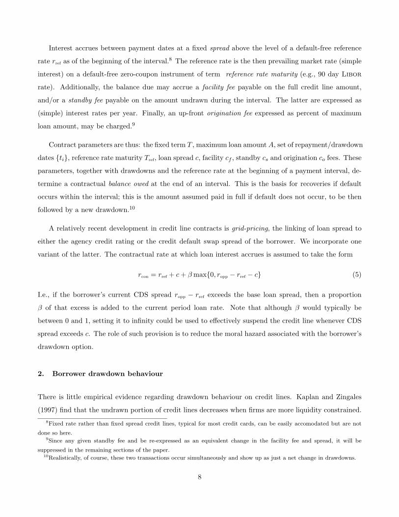
Figure 2 graphs line values. Unlike the extremes considered so far, line value is no longer monotonic
in contractual spread, as seen from the curved line value curve along the loan spread dimension. For
borrowers with credit quality of 6, line value reaches a maximum value of $0.86 at c of approximately 6%.
12

For borrowers with credit quality of 8, line value reaches a maximum value of $2.76 at c of approximately
6%. Above these levels, the reduction in balances on which the spread is received more than outweighs the
increase in spread and reduction in default losses. The reverse happens as spreads are reduced. Similar
to the previous cases, line value is positively related to the borrower’s initial credit quality. The loan
value in this case is lower than in the zero drawdown scenario, but higher than in the high drawdown
case. Under an intermediate drawdown rate, the borrower only exercises part of the embedded option.
Hence the loan presents a higher cost to the lender than the no optionality case (no sensitivity) and lower
cost than the total optionality case (high sensitivity).
Panel B of Table 5 reports loan values suppressing jumps in credit quality. Similar to the last two
cases, ignoring jumps leads to overvaluation.
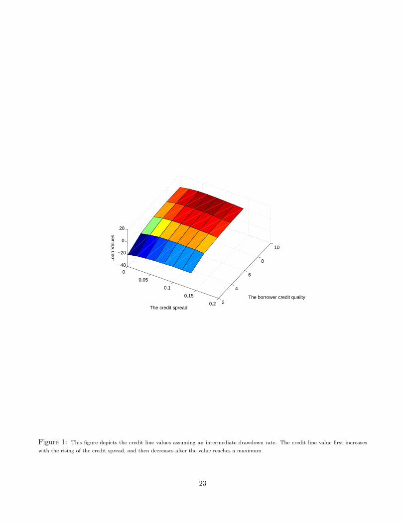
Table 6 gives credit exposure measures and initial drawdown ratios of loans. Figure 3 gives some
sense of how much drawdowns vary with loan spread and credit quality.
Figure 4 depicts the bond-equivalent exposure measure for different loan spread and borrower credit
qualities. Noteworthy here is that the bond-equivalent measure is typically far larger than the initial
drawdown. E.g., for a borrower with credit quality of 6 and a contractual spread of 4%, the bond-
equivalent risk exposure is $80.34, while the initial drawdown is only $32.4. The CDS values in Panel
B report that it would cost $3.22 to compensate the lender for default risk for this specific borrower.
An important lesson learned is that the credit exposure over the life of credit lines is far greater than
the initial drawdown would suggest. This suggests that it would be inaccurate to use either the current
drawdown or the full line limit as measure of the line’s credit exposure.
The drawdowns in Panel C confirm smaller line utilization the higher is either borrower credit quality
or loan spread.
4. Break-even loan spreads
This experiment investigates how break-even loan spreads relate to drawdown sensitivity. We get a
different perspective from looking at the lowest contractual spread for which line value is 0. Panel A of
Table 7 displays this spread for a range of dsen values and initial credit qualities. For each credit quality,
however, there is a size of dsen beyond which there is no spread that can make the line break even for
the lender. In other words, without origination, facility, standby fees, or a shortening of maturity, there
13

are no terms under which the lender can rationally grant the borrower a revolving credit line. This again
explains why a multiple fee structure is typically used in practice.
Panel B reports the correponding fair spreads when an origination fee cu=$2 is added. Comparison
of Panel A and B shows that the addition of origination fees permits a definitely negative value loan to
become zero value. I.e., the non-existence of the fair credit spread problem is overcome by addition of the
origination fee. For instance, when dsen = 3 and the borrower has credit quality of 4, without origination
fee no fair credit spread exists. This indicates that the loan poses negative value to the lender no matter
how high a spread is charged. However, with the addition of the origination fee, the fair credit spread
becomes 6.21%. Confirmed by many unreported numerical experiments, this shows the complementarity
of fees and also justifies the necessity of multiple fees.
Panel C of Table 7 reports credit line values for different drawdown sensitivities and credit quality
combinations assuming a loan spread of 2%. Two interesting features are confirmed. First, loan value
is negatively related to drawdown sensitivity. E.g., for a loan made to borrower with a credit quality of
6, loan value is $-0.74 when dsen = 1 and $-1.45 when dsen = 11. Second, the loan values are negative
when the credit spread is lower than the fair credit spread, and positive otherwise. For cases in which
the fair credit spread is less than 2%, the lender is over-pricing the loan, hence the loan delivers positive
value. For cases in which fair credit spread is more than 2%, the lender is under-pricing the loan, and
the loan delivers negative value. For example, the fair credit spreads with a drawdown sensitivity of 3
(Panel A) are 2.88% for credit quality of 6 and 0.91% for credit quality of 8. In Panel B for the same
drawdown sensitivity of 3, the credit line made to borrowers with credit quality of 6 is under-priced and
has negative loan values of $-0.91. The loan made to borrowers with credit quality of 8 are over-priced
and has a positive loan value of $1.27.
IV. Conclusion
Revolving lines of credit are the most import channel for banks to provide business loans. We propose
a broadly applicable, computationally tractable, credit line valuation framework, that considers both
gradual and sudden change in credit quality. Through numerical examples, we illustrate important
characteristics of credit line pricing. First, credit line value depends critically on drawdown sensitivity.
The higher the sensitivity, the more costly the loan. Second, the break-even spread increases with
drawdown sensitivity. For each credit quality, however, there is a level of drawdown sensitivity beyond
14

which there is no spread that can make the line break even for the lender. Hence multiple fees may
be required for a mutually beneficial contract to be reached. Third, loan value does not necessarily
monotonically increase with loan spread. A higher credit spread can reduce credit line value due to
reduction in line usage. Lastly, it can be costly to the lender to ignore the possibility of a sudden credit
quality change.
The setup of the model is sufficiently flexible to allow it to reflect different fee structures and loan
characteristics. Parameters of the model can be calibrated using empirical bond pricing data.
Our model also produces two important measures for a revolving credit line’s exposure to default
risk. The first measure is the line’s bond-equivalent, which expresses the credit exposure as the principal
amount of constant balance floating rate loan of the same term with identical credit default swap cost.
This measure is lower than the loan limit for credit lines, but typically much higher than current draw-
downs. This measure more accurately reflects the risk exposure of credit lines over the life of the loan.
It generally lay between 70 and 100% of the loan limit. Second, we calculate credit exposure using the
up-front cost of an associated CDS. Though very small for borrowers of high quality, it rapidly escalates
with declines in credit quality. This provides an exposure measure from a different perspective as well as
providing useful information for financial professionals to price such derivative products.
15

Appendix A: Numerical solution for security values
We obtain an approximate numerical solution for V (s, r, t) by recursively working back from contract
maturity T in a discretized state space. We will treat r as deterministic in the current paper. Discount
factors R(ti) can thus be calculated directly and consideration of the r state is suppressed. We solve for
V on a uniformly spaced rectangular grid on [0, T ] × [smin, smax] with mesh size h in the s direction and
k in the t direction, chosen so that payment dates lie at gridpoints. Since we also take recoveries to be
independent of how negative is s, we let smin = 0 correspond to the default barrier. smax is chosen to be
a large enough that exceeding it from initial s(0) of interest within time T is sufficiently unlikely.11 Let
Vij , i = 0 . . . I, j = 0 . . . J be the solution at credit quality step i up from the default barrier and time
step j away from origination. Vector Vj denotes the solution at time step j. Its length is the number of
states considered in the s-direction.
The maturity value V (s, r, T ), conditional no prior default, is assumed known from the contract terms
and used to fill in values in the terminal vector VJ . We work backward one timestep k by treating the
jump and diffusion changes in s as occuring in sequence: I.e., within each interval all changes in s from
diffusion over time k occur first, with no jumps; then all jumps in s over time k occur, with no diffusion.
The diffusion part is handled by applying the Crank-Nicholson finite difference method to a the
vector of s-contingent values, just as if the jump process were not present, with boundary condition at
smin imposed by recovery value ρB. The partial differential equation being solved is what one gets from
the Feynman-Kac formula for conditional expected value,
12σ2Vss + αVs + Vt = 0 (7)
At the upper boundary we use the (technically incorrect) expedient of assuming V to be quadratic in s.
I.e., the value of Vj at smax is the quadratic extrapolation of its values at the three neighbouring interior
gridpoints. In certain cases, if the value of the security were it default-free is known, it works better to
suppose that default is effectively inaccessible from smax and impose that as a known-value condition at
that edge. The result of this step is to multiply vector Vj by some matrix C.
The jump part is handled by constructing a transition matrix M over s-states approximating the
changes from this source over interval k. This matrix is pre-calculated as follows. Choose a modest sized
integer n, and approximate the Poisson process over a subinterval of length k/2n by supposing at most11This obviously will depend on the particulars of the processes involved and the relative magnitude of cash flows in
different regions of the state space.
16

one jump occurs in that subinterval. From a particular level si on the grid, the probability of one jump is
λ(si)k/2n. If that occurs, the probability of moving to level sl is taken to be F (sl + 12h, si)−F (sl− 1
2h, si).
I.e., it is assumed that jumps are exclusively to gridpoints. The subinterval jump transition probabilities
are thus12
prob{sl|si} =
{1− (1− F (si + 1
2h, si) + F (si − 12h, si))λ(si)k/2n for l = i
(F (sl + 12h, si)− F (sl − 1
2h, si))λ(si)k/2n for l 6= i(8)
The resulting matrix is then squared n times to get the transition matrix M (which allows for up to n
jumps) over interval k.13
Discounting by the default-free rate over time interval [(j − 1)k, jk] is accomplished by multiplying
the result (for the non-default s levels) by the s-independent quantity
dj ≡ e−∫ jk(j−1)k
r(x) dx
We thus get
Vj−1 = djCMVj (9)
In practice, computation costs are reduced by treating as 0 elements of M below some threshold (e.g.,
10−10), storing the rescaled result as a sparse matrix, and using a sparse matrix multiplication routine.
The ‘multiplication by C’ is done by solving the tridiagonal equation system that comes out of the Crank-
Nicolson algorithm. Computation costs per time step are thus typically much less than a single matrix
multiplication of Vj .14
One proceeds thus back from time T , pausing at each payment date ti to add to each element of Vj
the s-contingent contractual payment received by the lender in non-default states. Security values for s
not at gridpoints is found by (cubic) interpolation on V0.
Appendix B: Parameter estimation
A fixed rate non-callable bond is a simple contract. In valuation equation (3), {ti} are the coupon
payment dates remaining, q(s, r, ti) equal the fixed coupon payments (plus maturity value at T ), and B
12Jumps to below smin are treated as being to smin and to above smax as being to smax.13The alternative of allowing for arbitrarily large number of jumps in interval k would require calculating the eigenvalues
and eigenvectors of the I × I matrix of infinitesimal transition probabilities, which would be computationally more costly.14We are losing something by ignoring the interaction of jump and diffusion within the interval when the components of
each depends on s. A more ‘centered’ approximation over interval k can be achieved by doing M1/2CM1/2 rather than CM .
17

is the par value plus (linearly) accrued interest at default time τ . For given model parameters θ and
credit state for firm i at month j of sij , let Vijk denote the (numerically computed) theoretical value of
bond k of that firm.15 Let Pijk denote the corresponding actual market price quote (plus accrued interest
to transaction settlement date). Let dijk denote the Hicks/Macauly duration of bond ijk (sensitivity of
value to its own annualized yield to maturity). The parameter estimation criterion was to find θ, {sij}
minimizing the weighted sum-squared-residuals
S ≡∑i,j,k
(Pijk − Vijk
dijk
)2
(10)
subject to the constraints ∑k
Pijk − Vijk
dijk= 0 ∀ i, j (11)
The deflating of price residuals by duration expresses the residuals (approximately) in terms of difference
between quoted yield to maturity and the model’s forecast; if not done, the short end of the maturity
spectrum would have little influence. Constraints (11) assert that market and model yields, averaged over
all bonds of a given firm outstanding on a given day, agree exactly. This identifies the credit state, and
renders sij , conditional on θ, observable without error—one way of handling the latent variable problem
were we to bring time series properties of s into the estimation.16 Minimization of S over θ was done
using Marquardt’s algorithm, extended to incorporate bounds on parameter values to make the search
better behaved.
Notice that we make no use of actual time series properties of bond prices here. Data dates could
be shuffled with no effect. The basic question is whether a small set of fixed parameters—common to
all firms and all points in time—combined with a single firm-and-date-specific variable s can reasonably
capture all ‘term structures of credit spreads’ observed. Equivalently, since it is only the risk-neutral
density of time to default that matters for the bond values, can the one-dimensional family of density
functions implied by the specification adequately explain observed prices?
For the data set available, within the contraints of the specification chosen, not all parameters were
well identified. To cut the story short (and the computational intensity), we imposed the following:
recovery rate ρ = .5, roughly consistent with Altman and Kishore’s (1996) reported average for US15Also needed for this calculation is that date’s default-free yield curve, taken from the constant maturity US Treasury
yield curve as mentioned earlier.16See Honore (1998) and Jones and Wang (1996) for previous use of this method.
18

corporate bonds;17 κ = 0, so no mean reversion; σ = 1.0 (per year), viewed as an almost free scaling
parameter. The four remaining parameters were estimated with the following results:
λ0 .48 κ 0.0
δ .38 s̄ —
s̄a 1.10 σ 1.0
σa .80 ρ 0.5
(12)
Here s̄a and σa are the mean and standard deviation of the uniform distribution on absolute jump
destination. I.e., F is uniform on the interval [s̄a − 31/2σa, s̄a − 31/2σa] = [−.286, 2.49].
These parameters give quite a good fit to the observed bond prices. Standard deviation of the price
residuals is .70 (on par value of 100). Expressed as yield to maturity residuals, 53% of observations are
below 5 basis points, 77% are below 10 bp, 95% are below 25 bp, 99% are below 50 bp.
The credit state s(t) can be given more tangible interpretation in terms of the fair credit spread on
instantaneously maturing loans. Very short term loans can only default through jump. Expected default
losses over an interval of length dt are thus (1− ρ)λ(s)F (0, s) dt, the product of the loss rate in default,
probability of a jump occuring, and probability that the jump would land in the default region.
Fair credit spreads for longer maturities must allow for diffusion of s both to default directly and to
levels with different jump intensities. They are typically much larger than the instantaneous spread above.
For currently high quality borrowers, credit spread increases with maturity; for low quality borrowers,
after an initial hump occuring somewhere before two years, credit spread declines with maturity.
Time series analysis of the estimated sij showed them to have small drift (.072/yr), slight negative first
order serial correlation (-.067 for monthly observations), and diffusion volatility of σ of 0.57 . The latter
was noticeably below the value of 1.0 assumed, so σ was reset to 0.75 and the parameters re-estimated,
with better consistency between the assumed and realized σ.
Appendix C: Numerical solution for line value
Valuation of the credit line proceeds as in section IV. with some modification. We must accomodate the
fact that the size of drawdown is determined by s at the beginning of a payment interval, but whether
one gets paid is determined by s at the end. Moreover the interest rate charged over the interval is17They report mean recovery rate for senior secured notes of 57.94%, with standard deviation of 23.12%; and mean
recovery rate for senior unsecured notes of 47.70%, with standard deviation of 26.60%.
19

based on rref prevailing at the start. Thus cash flows at ti are determined by the r, s state at both ti and
ti−1 jointly.18 This is handled as follows. Between payment dates, the vector Vj recursively solved for
is the value of the credit line’s cash flows from the next payment date onwards, as a function of current
s, conditional on no default prior to that time. If s = 0 currently, then all future cash flows will be
zero, captured by imposing boundary condition V (0, r, t) = 0 for t not in {ti}. Let ∆ ≡ ti+1 − ti be the
payment interval. If t is a payment date ti, then for each s in our discretized state space we calculate
rref, ropp, gap g, and the fair value p of a unit discount bond of maturity ∆ issued by the borrower with
the same recovery rate as the credit line. We add to Vj(s) the amount
−Af(g) + pA (f(g)(1 + (rref + c− cs)∆) + (cs + cf )∆) (13)
First term is the cash paid out as current drawdown; second term is expectedQ discounted value of the
contractual payments now due at ti+1. At s = 0 this treats the borrower as drawing down, defaulting
right away, and providing immediate recoveries a proportion of the balance due at the next payment date.
For equal length payment intervals the vector of risky bond values p(s), up to a riskless rate discount
factor independent of s, need only be computed once.
Solution for the breakeven loan spread is done by interative search (using secant method) over values
of c until spread giving 0 loan value is found.
References
[1] Berkovitch, Elazar and Stuart Greenbaum (1991). The Loan Commitment as an Optimal Financing
Contract. Journal of Financial and Quantitative Analysis, March, 83-95.
[2] Boot, A.. A.V. Thakor and G. Udell, (1987). Competition, risk neutrality and loan commitments.
Journal of Banking and Finance 11, 449-471.
[3] Campbell, T.S., (1978). A model of the market for lines of credit. Journal of Finance 33, 231-244.
[4] Duffie, Darrell, and Kenneth J. Singleton, (1997). An Econometric Model of the Term Structure of
Interest-Rate Swap Yields. Journal of Finance, 52 no. 4, 1287-1321.
[5] Duffie, D. (2001). Dynamic Asset Pricing Theory, 3rd ed., Princeton University Press.18The payment of interest in arrears is not a problem in the current deterministic interest rate setting, but would become
so if the default-free rate were treated as stochastic.
20

[6] Gatev, Evan and Philip Strahan (2006). Banks Advantage in Hedging Liquidity Risk: Theory and
Evidence from the Commercial Paper Market. Journal of Finance 61, 867-892.
[7] Holmstrom, Bengt and Jean Tirole (1998). Private and Public Supply of Liquidity. Journal of Po-
litical Economy 106, 1-40.
[8] Hughston, L. P. and S. M. Turnbull (2002). Pricing Revolvers. Working Paper, available from the
second author.
[9] James, C., (1982). An analysis of bank loan rate indexation. Journal of Finance 37, 809-825.
[10] Jarrow, R. A. and S. M. Turnbull (1995). The Pricing and Hedging of Options on Financial Securities
Subject to Credit Risk. Journal of Finance, 50(1), 53-85.
[11] Jarrow, R. A. and S. M. Turnbull (1997). An Integrated Approach to the Hedging and Pricing of
Eurodollar Derivatives. Journal of Risk and Insurance, 64(2), 271-99.
[12] Jones, R. A. (2001), Analyzing Credit Lines With Fluctuating Credit Quality, Working Paper,
Department of Economics, Simon Fraser University.
[13] Kanatas, G., 1987, Commercial paper, bank reserve requirements and the informational role of loan
commitments, Journal of Banking and Finance 11, 425-448.
[14] Kane, Edward, 1974, All for the best: The Federal Reserve Boards 60th annual report. American
Economic Review 64, 835-850.
[15] Kaplan, Steven and Luigi Zingales (1997). Do Investment-Cash Flow Sensitivities Provide Useful
Measures of Financing Constraints? Quarterly Journal of Economics 112, 169-215.
[16] Kashyap, A. K., Rajan, R. and J. Stein, (2002). Banks as Liquidity Providers: An Explanation for
the Coexistence of Lending and Deposit-Taking. Journal of Corporate Finance 57, 33-73
[17] Loukoianova, E., Neftci, S. N. and S. Sharma (2006). Pricing and Hedging of Contingent Credit
Lines. IMF Working Paper.
[18] Melnik, A. and S.E. Plaut, 1986. The economics of loan commitment contracts: Credit pricing and
utilization. Journal of Banking and Finance 10, 267-280.
[19] Sufi, A. (2006). Bank Lines of Credit in Corporate Finance: An Empirical Analysis. Working Paper,
FDIC Center for Financial research
[20] Saidenberg, M. R., and P. E. Strahan, (1999). Are banks still important for financing large busi-
nesses? Current Issues in Economics and Finance 5(12), 16, Federal Reserve Bank of New York.
21

[21] Shockley, R. and A. Thakor, (1997). Bank Loan Commitment Contracts: Data, Theory, and Tests.
Journal of Money, Credit and Banking 29, 4, 517-534.
[22] Thakor, A.V., (1982). Toward a theory of bank loan commitments. Journal of Banking and Finance
6, 57-83.
[23] Thakor, A.V. and G.F. Udell (1987). An economic rationale for the pricing structure of bank loan
commitments. Journal of Banking and Finance 11, 271-289.
[24] Turnbull, S. M. (2003). Pricing Loans Using Default Probabilities. Economic Notes, 32(2), 197-217.
22
0
0.05
0.1
0.15
0.2 2
4
6
8
10
−40
−20
0
20
The borrower credit quality
The credit spread
Loan
Val
ues
Figure 1: This figure depicts the credit line values assuming an intermediate drawdown rate. The credit line value first increases
with the rising of the credit spread, and then decreases after the value reaches a maximum.
23

0
0.05
0.1
0.15
0.2 2
4
6
8
10
0
20
40
60
The borrower credit quality
The credit spread
perc
enta
ge d
raw
dow
n
Figure 2: This figure depicts the credit line drawdown proportion assuming an intermediate drawdown rate. The drawdown
proportion is negatively related to the credit spread of the credit lines as well as the borrower’s initial credit quality.
24
0
0.05
0.1
0.15
0.2 2
4
6
8
10
60
80
100
The borrower credit quality
The credit spread
The
Bon
d E
quiv
alen
t Cre
dit E
xpos
ure
Figure 3: This figure depicts the credit line bond-equivalent risk exposure assuming an intermediate drawdown rate. The bond-
equivalent, similar to the initial drawdown, is negatively related to the credit spread of the credit lines as well as t
25

Table 1: Term structure of credit spreads
1 mo. 6 mo. 1 yr. 2 yr. 3 yr. 5 yr. 10 yr. 20 yr.
prob. default (%) 0.06 0.51 1.26 3.24 5.7 11.66 27.81 50.32
dsen=0 0.36 0.86 1.06 1.31 1.50 1.77 2.08 2.12
dsen=1 0.36 1.36 1.75 2.24 2.59 3.14 3.78 3.87
dsen=2 0.36 1.38 1.80 2.33 2.73 3.35 4.12 4.23
dsen=3 0.36 1.41 1.85 2.44 2.88 3.61 4.59 4.75
dsen=4 0.36 1.44 1.91 2.56 3.08 4.01 5.52 5.88
Note: The table reports the fair contractual spread and default probabilities for credit lines of
various maturities and drawdown sensitivities. The base case assumes a 3 year credit line with the
contractual maximum balance A = 100; one month (Topp = Tref = .0833 yr); origination, facility
and standby fees are 0. Recovery rate in default is ρ = 0.5. The default-free term structure is
assumed flat at 5%/yr, continuously compounded. The initial credit state of the borrower S(0) = 6.
26

Table 2: Line Value with Zero DrawDown Sensitivity
c 2% 4% 6% 8% 10% 12% 14%
s A: Line Values With Credit Quality Jump ($)
2 -8.98 -6.86 -4.73 -2.61 -0.49 1.64 3.76
4 -2.12 0.42 2.96 5.5 8.04 10.57 13.11
6 0.67 3.35 6.03 8.71 11.39 14.06 16.74
8 2.04 4.78 7.53 10.27 13.02 15.76 18.72
10 2.66 5.43 8.21 10.98 13.76 16.53 19.31
B: Line Values Without Credit Quality Jump ($)
2 -4.46 -2.04 0.38 2.8 5.22 7.64 10.06
4 2.15 4.92 7.68 10.45 13.21 15.97 18.74
6 2.76 5.54 8.32 11.1 13.88 16.66 19.44
8 2.78 5.56 8.34 11.12 13.9 16.68 19.46
10 2.78 5.56 8.34 11.12 13.9 16.68 19.46
Note: The table reports credit line values calculated numerically under different credit spreads c and
the borrower’s initial credit quality s, assuming zero drawdown sensitivity. The base case assumes a
3 year credit line with the contractual maximum balance A = 100; payment interval, reference and
opportunity cost rate maturities of one month (Topp = Tref = .0833 yr); origination, facility and
standby fees are 0. Recovery rate in default is ρ = 0.5. The default-free term structure is assumed
flat at 5%/yr, continuously compounded.
27

Table 3: Credit exposures: Bond-equivalent and CDS value (dsen = 0)
c 2% 4% 6% 8% 10% 12% 14%
s A: Bond Equivalent ($)
2 50 50 50 50 50 50 50
4 50 50 50 50 50 50 50
6 50 50 50 50 50 50 50
8 50 50 50 50 50 50 50
10 50 50 50 50 50 50 50
B: Value of credit default swap ($)
2 11.1 11.1 11.1 11.1 11.1 11.1 11.1
4 4.66 4.66 4.66 4.66 4.66 4.66 4.66
6 2 2 2 2 2 2 2
8 0.71 0.71 0.71 0.71 0.71 0.71 0.71
10 0.12 0.12 0.12 0.12 0.12 0.12 0.12
Note: The table reports the bond-equivalent and the cost of credit swap for credit lines with different
credit spreads c and the borrower’s initial credit quality s, assuming zero drawdown sensitivity. The
base case assumes a 3 year credit line with the contractual maximum balance A = 100; payment
interval, reference and opportunity cost rate maturities of one month (Topp = Tref = .0833 yr);
origination, facility and standby fees are 0. Recovery rate in default is ρ = 0.5. The default-free
term structure is assumed flat at 5%/yr, continuously compounded.
28
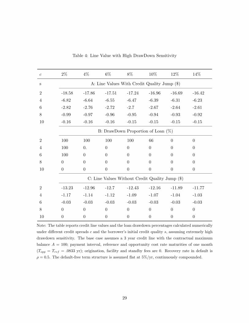
Table 4: Line Value with High DrawDown Sensitivity
c 2% 4% 6% 8% 10% 12% 14%
s A: Line Values With Credit Quality Jump ($)
2 -18.58 -17.86 -17.51 -17.24 -16.96 -16.69 -16.42
4 -6.82 -6.64 -6.55 -6.47 -6.39 -6.31 -6.23
6 -2.82 -2.76 -2.72 -2.7 -2.67 -2.64 -2.61
8 -0.99 -0.97 -0.96 -0.95 -0.94 -0.93 -0.92
10 -0.16 -0.16 -0.16 -0.15 -0.15 -0.15 -0.15
B: DrawDown Proportion of Loan (%)
2 100 100 100 100 66 0 0
4 100 0. 0 0 0 0 0
6 100 0 0 0 0 0 0
8 0 0 0 0 0 0 0
10 0 0 0 0 0 0 0
C: Line Values Without Credit Quality Jump ($)
2 -13.23 -12.96 -12.7 -12.43 -12.16 -11.89 -11.77
4 -1.17 -1.14 -1.12 -1.09 -1.07 -1.04 -1.03
6 -0.03 -0.03 -0.03 -0.03 -0.03 -0.03 -0.03
8 0 0 0 0 0 0 0
10 0 0 0 0 0 0 0
Note: The table reports credit line values and the loan drawdown percentages calculated numerically
under different credit spreads c and the borrower’s initial credit quality s, assuming extremely high
drawdown sensitivity. The base case assumes a 3 year credit line with the contractual maximum
balance A = 100; payment interval, reference and opportunity cost rate maturities of one month
(Topp = Tref = .0833 yr); origination, facility and standby fees are 0. Recovery rate in default is
ρ = 0.5. The default-free term structure is assumed flat at 5%/yr, continuously compounded.
29

Table 5: Line Value with Intermediate DrawDown Sensitivity
c 2% 4% 6% 8% 10% 12% 14%
s A: Line Values With Credit Quality Jump ($)
2 -18.03 -16.16 -15.02 -14.49 -14.39 -14.55 -14.82
4 -5.63 -4.01 -3.24 -3.14 -3.46 -3.98 -4.54
6 -1.05 0.34 0.86 0.76 0.28 -0.36 -0.99
8 1.08 2.35 2.76 2.55 2.00 1.31 0.66
10 2.04 3.25 3.61 3.36 2.77 2.07 1.40
B: Line Values Without Credit Quality Jump ($)
2 -11.42 -10.1 -9.51 -9.43 -9.67 -10.04 -10.42
4 1.04 2.25 2.62 2.40 1.83 1.15 0.51
6 2.20 3.39 3.74 3.48 2.89 2.18 1.51
8 2.23 3.43 3.77 3.51 2.92 2.21 1.54
10 2.23 3.43 3.77 3.51 2.92 2.21 1.54
Note: The table reports credit values calculated numerically under different credit spread c and
the borrower’s initial credit quality s, assuming intermediate drawdown sensitivity. The base case
assumes a 3 year credit line with the contractual maximum balance A = 100; payment interval,
reference and opportunity cost rate maturities of one month (Topp = Tref = .0833 yr); origination,
facility and standby fees are 0. Recovery rate in default is ρ = 0.5. The default-free term structure
is assumed flat at 5%/yr, continuously compounded.
30
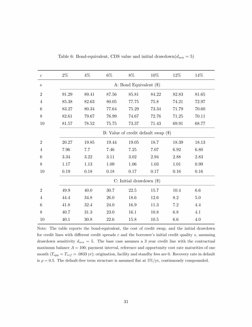
Table 6: Bond-equivalent, CDS value and initial drawdown(dsen = 5)
c 2% 4% 6% 8% 10% 12% 14%
s A: Bond Equivalent ($)
2 91.29 89.41 87.56 85.81 84.22 82.83 81.65
4 85.38 82.63 80.05 77.75 75.8 74.21 72.97
6 83.27 80.34 77.64 75.29 73.34 71.79 70.60
8 82.61 79.67 76.99 74.67 72.76 71.25 70.11
10 81.57 78.52 75.75 73.37 71.43 69.91 68.77
B: Value of credit default swap ($)
2 20.27 19.85 19.44 19.05 18.7 18.39 18.13
4 7.96 7.7 7.46 7.25 7.07 6.92 6.80
6 3.34 3.22 3.11 3.02 2.94 2.88 2.83
8 1.17 1.13 1.09 1.06 1.03 1.01 0.99
10 0.19 0.18 0.18 0.17 0.17 0.16 0.16
C: Initial drawdown ($)
2 49.9 40.0 30.7 22.5 15.7 10.4 6.6
4 44.4 34.8 26.0 18.6 12.6 8.2 5.0
6 41.8 32.4 24.0 16.9 11.3 7.2 4.4
8 40.7 31.3 23.0 16.1 10.8 6.8 4.1
10 40.1 30.8 22.6 15.8 10.5 6.6 4.0
Note: The table reports the bond-equivalent, the cost of credit swap, and the initial drawdown
for credit lines with different credit spreads c and the borrower’s initial credit quality s, assuming
drawdown sensitivity dsen = 5. The base case assumes a 3 year credit line with the contractual
maximum balance A = 100; payment interval, reference and opportunity cost rate maturities of one
month (Topp = Tref = .0833 yr); origination, facility and standby fees are 0. Recovery rate in default
is ρ = 0.5. The default-free term structure is assumed flat at 5%/yr, continuously compounded.
31
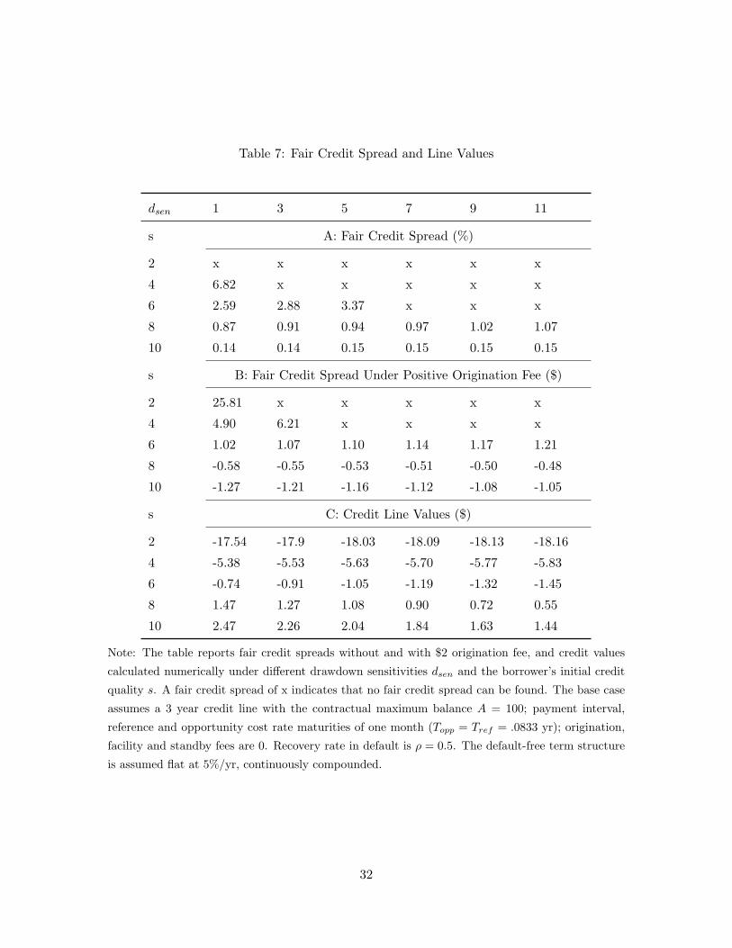
Table 7: Fair Credit Spread and Line Values
dsen 1 3 5 7 9 11
s A: Fair Credit Spread (%)
2 x x x x x x
4 6.82 x x x x x
6 2.59 2.88 3.37 x x x
8 0.87 0.91 0.94 0.97 1.02 1.07
10 0.14 0.14 0.15 0.15 0.15 0.15
s B: Fair Credit Spread Under Positive Origination Fee ($)
2 25.81 x x x x x
4 4.90 6.21 x x x x
6 1.02 1.07 1.10 1.14 1.17 1.21
8 -0.58 -0.55 -0.53 -0.51 -0.50 -0.48
10 -1.27 -1.21 -1.16 -1.12 -1.08 -1.05
s C: Credit Line Values ($)
2 -17.54 -17.9 -18.03 -18.09 -18.13 -18.16
4 -5.38 -5.53 -5.63 -5.70 -5.77 -5.83
6 -0.74 -0.91 -1.05 -1.19 -1.32 -1.45
8 1.47 1.27 1.08 0.90 0.72 0.55
10 2.47 2.26 2.04 1.84 1.63 1.44
Note: The table reports fair credit spreads without and with $2 origination fee, and credit values
calculated numerically under different drawdown sensitivities dsen and the borrower’s initial credit
quality s. A fair credit spread of x indicates that no fair credit spread can be found. The base case
assumes a 3 year credit line with the contractual maximum balance A = 100; payment interval,
reference and opportunity cost rate maturities of one month (Topp = Tref = .0833 yr); origination,
facility and standby fees are 0. Recovery rate in default is ρ = 0.5. The default-free term structure
is assumed flat at 5%/yr, continuously compounded.
32