Credit Booms Gone Bust: Monetary Policy, Leverage Cycles and Financial Crises, 1870–2008*

Moritz Schularick

Freie Universität Berlin†

Alan M. Taylor University of California, Davis, NBER, and CEPR‡

First version: November 2009 This version: February 2010

Abstract

The crisis of 2008–09 has focused attention on money and credit fluctuations, financial crises, and policy responses. In this paper we study the behavior of money, credit, and macroeconomic indicators over the long run based on a newly constructed historical dataset for 14 developed countries over the years 1870–2008, utilizing the data to study rare events associated with financial crisis episodes. We present new evidence that leverage in the financial sector has increased strongly in the second half of the twentieth century as shown by a decoupling of money and credit aggregates, and we also find a decline in safe assets on banks’ balance sheets. We show for the first time how monetary policy responses to financial crises have been more aggressive post-1945, but how despite these policies the output costs of crises have remained large. Importantly, we demonstrate that credit growth is a powerful predictor of financial crises, suggesting that such crises are “credit booms gone wrong” and that policymakers ignore credit at their peril. It is only with the long-run comparative data assembled for this paper that these patterns can be seen clearly.

JEL codes: E44, E51, E58, G01, G20, N10, N20. Keywords: banking, liquidity, central banking, monetary policy, financial stability.

* Some of this research was undertaken while Taylor was a visitor at the London School of Economics and a Houblon-Norman/George Fellow at the Bank of England. The generous support of both institutions is gratefully acknowledged. We thank Roland Beck, Warren Coats, Charles Goodhart, Carl-Ludwig Holtfrerich, Gerhard Illing, Christopher Meissner, Kris Mitchener, Eric Monnet, Andreas Pick, Hyun Shin, Solomos Solomou, Richard Sylla for helpful comments on a previous draft. All remaining errors are our own. † Email: moritz.schularick@fu-berlin.de. ‡ Email: amtaylor@ucdavis.edu.

1

In the brief history of macroeconomics, the subject of money and banking has witnessed wide fluctuations in both its internal consensus and external influence. The crisis of 2008–09 has reignited a new interest in understanding money and credit fluctuations in the macroeconomy and the crucial roles they could play in the amplification, propagation, and generation of shocks both in normal times and, even more so, in times of financial distress.

Research on the importance of financial structure promises to reopen a number of fundamental fault lines in modern macroeconomic thinking—between theories that treat the financial system as irrelevant, or, at least, not central to the understanding of economic outcomes, and those that reserve a central role for financial intermediation. In the monetarist view of Friedman and Schwartz (1963), but also in the recently dominant Neo-Keynesian synthesis (e.g., Woodford 2003) macroeconomic outcomes are largely independent of the performance of the financial system. On the other side, scholars such as Fisher (1933), Minsky (1978), Bernanke (1983, 1993), and Gertler (1988) have argued, to varying degrees, that financial factors can have a strong, distinct, and sometimes even dominant impact on the economy. Economic history has an important role to play in this debate, as a better empirical understanding can guide us toward the development of more useful economic theory. Critics have argued that theories detached from careful empirical science, based on deductive rather than inductive reasoning, have lost much of their aura (Eichengreen 2009), and this sentiment has been echoed after the crisis in the The Economist, The Financial Times, and other media. Thus, the failure of understanding revealed by the present crisis demands that we humbly return to macroeconomic and financial history, in the hope that more and better evidence may provide more useful guidance than introspection alone. Still, for other, more pragmatic reasons a return to the past is inevitable, because “rare events” of necessity thrust comparative economic history to the fore. If, notwithstanding the so-called Great Moderation, regular business cycles are roughly once per decade events, then we already have very few observations in the postwar data for any given country. More disruptive events like depressions and financial crises are rarer still, at least in developed economies. When sample sizes are this small, providing a detailed quantitative rendition, or even just a sketch of the basic stylized facts, requires that we work on a larger canvas, expanding our dataset across both time and space.

Hence, scholars have reached back to make careful comparisons with not just with past decades, but past centuries, using formal statistical analysis to examine the nature of financial crises and other rare events with new panel datasets, as in recent work by Reinhart and Rogoff (2009), Barro (2009), and Almunia et al. (2009). In the same spirit, the purpose of this paper is to step back and ask such questions about money, credit, and the macroeconomy in the long run. As a key part of this effort, we present a new long-run historical dataset for 14 developed countries over almost 140 years which will provide not just the empirical backbone for our research agenda but also serve as a valuable resource for future investigations by other scholars interested in this subject.

2

1. Three Views of Money and Credit

As quantitative historians we want to know whether the structures and dynamics of money, credit and the macroeconomy have shifted in the long run—and, how, and with what effects. To understand why this is still an important open question, we must also heed the intellectual historians who ask where the debate stands and how we got here.

To oversimplify for the sake of brevity, the relevant intellectual history might be reduced to three main viewpoints, and their associated periods of influence (see Freixas and Rochet 1997, chapter 6). The experience of the late nineteenth and early twentieth century, including the disruptions of the 1930s, formed the foundation of the “money view” which is indelibly associated with the seminal contributions of Friedman and Schwartz (1963). In this account, the level of the narrow and broad money supplies strongly influences output in the short run. The central bank can and must exert proper indirect control of aggregate bank liabilities, but beyond that, the actual functions of the banks, and their role in credit creation via bank loans, are of no great importance.

In the second half of the twentieth century the “irrelevance view” gained influence, associated with the ideas of Modigliani and Miller (1958) among others, where the details of the debt-equity financial structure of firms was inconsequential. Finance was a so-called veil. In this view, real economic decisions became independent of financial structure altogether. This gave intellectual underpinnings to later macroeconomic models like real business cycle theory and its offspring: models with money were rare, and models with any sort of financial structure were almost nonexistent. The influence of this view is still surprisingly strong, although it has been waning, and even more so after the recent crisis. Starting in the 1980s, the “credit view” has gradually attracted attention and adherents. In this view, starting with the works of Mishkin (1978), Bernanke (1983) and Gertler (1988), and drawing on ideas dating back to Fisher (1933) and Gurley and Shaw (1955), the mechanisms and quantities of bank credit matter, above and beyond the level of bank money.1 That is, the entire bank balance sheet, the asset side, leverage and composition, may have macroeconomic implications. One consequence may be an amplification of the monetary transmission mechanism, that is, a financial accelerator effect (Bernanke and Blinder 1988). Another issue might be the financial fragility effect induced by collateral constraints, where declining asset values impair lending, lowering productivity, thus causing further declines in asset values (Bernanke, Gertler, and Gilchrist 1999 or BGG). Still, one strand of criticism notes that in most of the financial-accelerator models credit remains by and large passive—as a propagator of shocks, not an independent source of shocks (Borio 2008; Hume and Sentance 2009). This was always well understood: for example, Bernanke and Gertler (1995, p. 28) stated that “[t]he credit channel is an enhancement mechanism, not a truly independent or parallel channel.”

1 This important turn in the literature in the 1980s was guided by more inductive empirical work, where important warnings about the role of credit included Eckstein and Sinai (1986) and Kaufman (1986).

3

Thus, the BGG benchmark model might appear to be too limited. A step forward is to introduce disturbances to the credit constraints in the BGG type of DSGE model (e.g., Nolan and Thoenissen 2009; Jermann and Quadrini 2009), although we then still need to know precisely what it is that drives the processes, or beliefs of agents, that lie behind such disturbances. More radical departures are possible in an older tradition; in the work of scholars such as Minsky (1978), the financial system itself is prone to generate economic instability through endogenous credit bubbles with waves of euphoria and anxiety. And indeed, economic historians such as Kindleberger (1978) have generally been sympathetic to such ideas pointing to recurrent episodes of credit-driven instability throughout financial history. In some models, multiple equilibria or feedback cycles are possible (Bernanke and Gertler 1995; Kiyotaki and Moore 1997). Recent work by Geanakoplos (2009) on the leverage cycle also meshes with this view.

2. Money, Credit, and Output in The Long Run Given these disparate views, we ask: what are the facts? To our knowledge, the dynamics of money, credit, and output have not been studied across a broad sample of countries over the long run. There are, however, a few recent studies that are comparable to ours in spirit, in that they lift the veil of finance to re-examine the link between financial structure and real activity in the past or present. Adrian and Shin (2008, 2009), Mendoza and Terrones (2008), as well as Hume and Sentance (2009) have analysed the structural changes in the financial system in recent years and the consequences for financial stability and monetary policy. Previously, Rousseau and Wachtel (1998) had investigated the link between economic performance and financial intermediation between 1870 and 1929 for five industrial countries, while Eichengreen and Mitchener (2003), among others, have studied the credit boom preceding the Great Depression.2

The contribution of this paper is to make a start on the broader, systematic, cross-country quantitative history of money and credit, by focussing on three main questions: (i) which key stylized facts can we derive from looking at the long-run trends in money and credit aggregates?; (ii) how have the responses of monetary and credit aggregates to financial crisis changed over time?; and (iii) what role do credit and money play as a cause of financial crises? Our empirical analysis proceeds as follows.

We first document and discuss our newly assembled dataset on money and credit, aligned with various macroeconomic indicators, covering 14 developed countries and the years from 1870 to 2008. This new dataset allows us to establish a number of important stylized facts about what we shall refer to as the “two eras of finance capitalism”. The first financial era runs from 1870 to 1939. In this era, money and credit were volatile but over the long run they maintained a roughly stable relationship to each other, and to the size of the economy measured by GDP. The only exception to this rule was the Great Depression period: in the 1930s money and credit aggregates collapsed. In this first era, the one studied by Friedman and Schwartz, the “money

2 A great number of postwar studies have focussed on the role of financial structure in comparative development and long-run economic growth, a question that is related but distinct from our analysis (Goldsmith 1969; Shaw 1973; McKinnon 1973; Jung 1986; King and Levine 1993).

4

view” of the world looks entirely plausible. However, the second financial era, starting in 1945, looks very different. First, money and credit began a long postwar recovery, trending up rapidly and then surpassing their pre-1940 levels compared to GDP by about 1970. That trend continued to the present and, in addition, credit itself then started to decouple from broad money and grew rapidly, via a combination of increased leverage and augmented funding via the nonmonetary liabilities of banks. In addition, we compare trends between Europe and the U.S. and other countries, finding that these trends are quite common across countries in the long run. We also show that there has been a rapid decline in “safe” assets on banks’ balance sheets, with the portfolio share of government securities declining dramatically since 1950, a trend which has added another element of risk. With the banking sector progressively more leveraged in the second financial era, particularly towards the end, the divergence between credit supply and money supply offers prima facie support for the credit view as against a pure money view; we have entered an age of unprecedented financial risk and leverage, a new global stylized fact that is not fully appreciated.

In a second empirical investigation we look at money, credit and the consequences of crises. We pursue an event-analysis approach to study the co-evolution of money and credit aggregates and real economic activity in the five year window following a financial crisis event, using a set of event definitions based on documentary descriptions in Bordo et al. (2001) and Reinhart and Rogoff (2009). We also pursue this analysis in two periods, 1870–1939 and 1945–2009; this is motivated by our identification of two distinct eras of finance, as above, but it also reflects the very different monetary and regulatory framework after WW2, namely the shift away from gold to fiat money, the greater role of activist macroeconomic policies, the greater emphasis on bank supervision and deposit insurance, and the expanded role of the Lender of Last Resort. Our results show dramatically different crisis dynamics in the two eras, or “now” versus “then.” In postwar crises, central banks have strongly supported money base growth, and crises have not been accompanied by a collapse of broad money. On the real side, a striking result is that the economic impact of financial crises is no more muted in the postwar era than in the prewar era. Thus, the real gains from financial stabilization policies may at first seem elusive, at least using the event analysis approach. The one caveat, here, is that given the much larger financial system we have today (the first stylized fact above) the real effects of the postwar regime could take the form of preventing the potentially even larger real output losses that could be realized in today’s more heavily financialized economies without such policies. With regard to prices, inflation has tended to rise after crises in the post-WW2 era, with economies avoiding the strong Fisherian debt-deflation mechanism that tended to operate in pre-WW2 crises, and this could be another factor preventing larger output losses.

The bottom line is that the lessons of the Great Depression, once learned, were put into practice. After 1945 financial crises were fought with a more aggressive monetary policy responses, banking systems imploded neither so frequently nor as dramatically, and deflation was avoided—although crises still had real costs. However, in tandem with our previous

5

findings, it is natural to ask to what extent the implicit and explicit insurance of financial systems by governments encouraged the massive expansion of leverage that emerged after the war.

In a final empirical exercise we ask what we can learn about the fragility of financial systems using our credit data. Specifically, we test one element of the credit view argument—associated with Minsky, Kindleberger, and others—that financial crises can be seen as “credit booms gone wrong.” To perform this test we follow the early-warning approach and construct a typical macroeconomic lagged information set at any date T for all countries in our sample. Lagged credit growth turns out to be highly significant as a predictor of financial crises, but the addition of any of the other variables adds very little explanatory power. These new results from long-run data, if they pass scrutiny, inform the current controversy over macroeconomic policy practices in developed countries. Specifically, the pre-2008 consensus argued that monetary policy should follow a “rule” based only on output gaps and inflation, but a few dissenters thought that credit aggregates deserved to be watched carefully and incorporated into monetary policy. The influence of the credit view has certainly advanced after the 2008–09 crash, just as respect has waned for the glib assertion that central banks could ignore potential financial bubbles and easily clean up after they burst.

3. The Data To study the long-run dynamics of money, credit and output we assembled a new annual dataset covering 14 countries over the years 1870–2008. The countries covered are the United States, Canada, Australia, Denmark, France, Germany, Italy, Japan, the Netherlands, Norway, Spain, Sweden, and the United Kingdom. At the core of our dataset are yearly data for aggregate bank loans and total balance sheet size of the banking sector. We complemented these credit series with narrow (M0 or M1) and broad (typically M2 or M3) monetary aggregates as well as data on nominal and real output, inflation and investment.

The two core definitions we work with are as follows. Total lending or bank loans is defined as the end-of-year amount of outstanding domestic currency lending by domestic banks to domestic households and non-financial corporations (excluding lending within the financial system). Banks are defined broadly as monetary financial institutions and include savings banks, postal banks, credit unions, mortgage associations, and building societies whenever the data are available. We excluded brokerage houses, finance companies, insurance firms, and other financial institutions. Total bank assets is then defined as the year-end sum of all balance sheet assets of banks with national residency (excluding foreign currency assets). It is important to point out that the definitions of credit, money, and banking institutions vary profoundly across countries, which makes cross-country comparisons difficult. In addition, in some cases such as the Netherlands or Spain, historical data cover only commercial banks, not savings banks or credit co-operatives. In this paper, we therefore focus predominantly on the time-series dimension of the data and for the most part avoid outright comparisons in levels (e.g.,

6

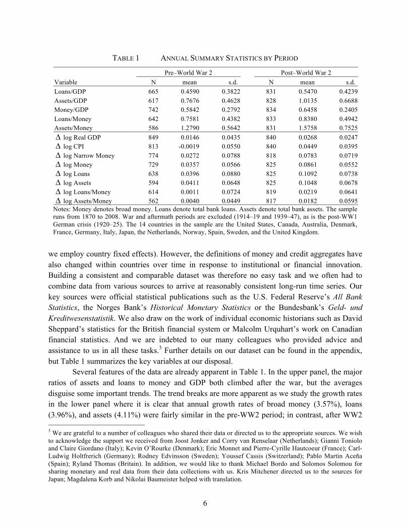
we employ country fixed effects). However, the definitions of money and credit aggregates have also changed within countries over time in response to institutional or financial innovation. Building a consistent and comparable dataset was therefore no easy task and we often had to combine data from various sources to arrive at reasonably consistent long-run time series. Our key sources were official statistical publications such as the U.S. Federal Reserve’s All Bank Statistics, the Norges Bank’s Historical Monetary Statistics or the Bundesbank’s Geld- und Kreditwesenstatistik. We also draw on the work of individual economic historians such as David Sheppard’s statistics for the British financial system or Malcolm Urquhart’s work on Canadian financial statistics. And we are indebted to our many colleagues who provided advice and assistance to us in all these tasks.3 Further details on our dataset can be found in the appendix, but Table 1 summarizes the key variables at our disposal.

Several features of the data are already apparent in Table 1. In the upper panel, the major ratios of assets and loans to money and GDP both climbed after the war, but the averages disguise some important trends. The trend breaks are more apparent as we study the growth rates in the lower panel where it is clear that annual growth rates of broad money (3.57%), loans (3.96%), and assets (4.11%) were fairly similar in the pre-WW2 period; in contrast, after WW2 3 We are grateful to a number of colleagues who shared their data or directed us to the appropriate sources. We wish to acknowledge the support we received from Joost Jonker and Corry van Renselaar (Netherlands); Gianni Toniolo and Claire Giordano (Italy); Kevin O’Rourke (Denmark); Eric Monnet and Pierre-Cyrille Hautcoeur (France); Carl-Ludwig Holtfrerich (Germany); Rodney Edvinsson (Sweden); Youssef Cassis (Switzerland); Pablo Martin Aceña (Spain); Ryland Thomas (Britain). In addition, we would like to thank Michael Bordo and Solomos Solomou for sharing monetary and real data from their data collections with us. Kris Mitchener directed us to the sources for Japan; Magdalena Korb and Nikolai Baumeister helped with translation.

TABLE 1 ANNUAL SUMMARY STATISTICS BY PERIOD

Pre–World War 2 Post–World War 2 Variable N mean s.d. N mean s.d. Loans/GDP 665 0.4590 0.3822 831 0.5470 0.4239 Assets/GDP 617 0.7676 0.4628 828 1.0135 0.6688 Money/GDP 742 0.5842 0.2792 834 0.6458 0.2405 Loans/Money 642 0.7581 0.4382 833 0.8380 0.4942 Assets/Money 586 1.2790 0.5642 831 1.5758 0.7525

€

∆ log Real GDP 849 0.0146 0.0435 840 0.0268 0.0247

€

∆ log CPI 813 -0.0019 0.0550 840 0.0449 0.0395

€

∆ log Narrow Money 774 0.0272 0.0788 818 0.0783 0.0719

€

∆ log Money 729 0.0357 0.0566 825 0.0861 0.0552

€

∆ log Loans 638 0.0396 0.0880 825 0.1092 0.0738

€

∆ log Assets 594 0.0411 0.0648 825 0.1048 0.0678

€

∆ log Loans/Money 614 0.0011 0.0724 819 0.0219 0.0641

€

∆ log Assets/Money 562 0.0040 0.0449 817 0.0182 0.0595 Notes: Money denotes broad money. Loans denote total bank loans. Assets denote total bank assets. The sample runs from 1870 to 2008. War and aftermath periods are excluded (1914–19 and 1939–47), as is the post-WW1 German crisis (1920–25). The 14 countries in the sample are the United States, Canada, Australia, Denmark, France, Germany, Italy, Japan, the Netherlands, Norway, Spain, Sweden, and the United Kingdom.

7

average broad money growth (8.61%) was much smaller than loan growth (10.92%) and asset growth (10.48%). The loan-money ratios grew at just 0.11% per year before WW2 but 2.19% per year after, a 20-fold increase in the growth rate of this key leverage measure. Similarly asset-money growth rates jumped from 0.40% to 1.82% per year, a quadrupling. Thus even at the level of simple summary statistics we can grasp that the behavior of money and credit aggregates changed markedly in the middle of the twentieth century. However, a more detailed analysis of these and other data brings the differences between the two eras into sharper relief.

4. Money and Credit in Two Eras of Finance Capitalism In a first step, we analyse the new dataset with an eye on deriving a number stylized facts about credit and monetary aggregates from the gold standard era until today.

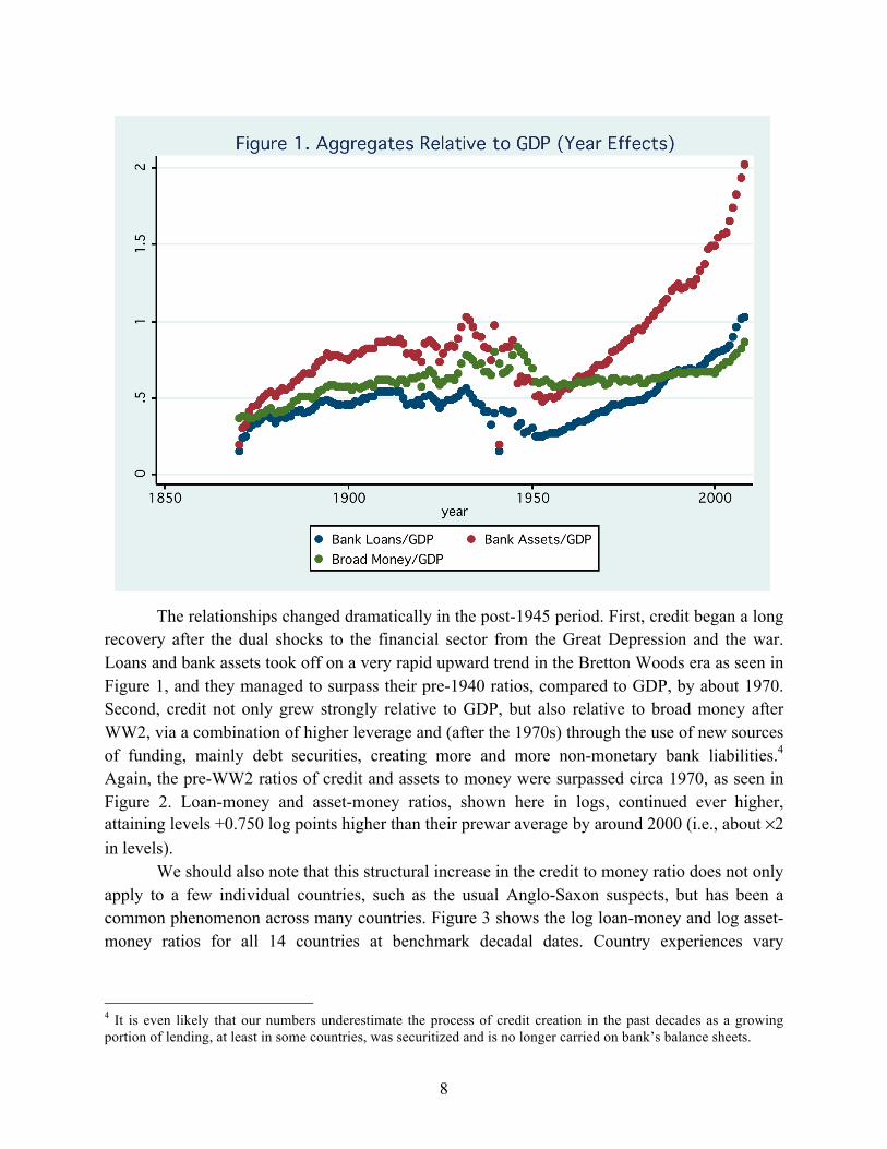
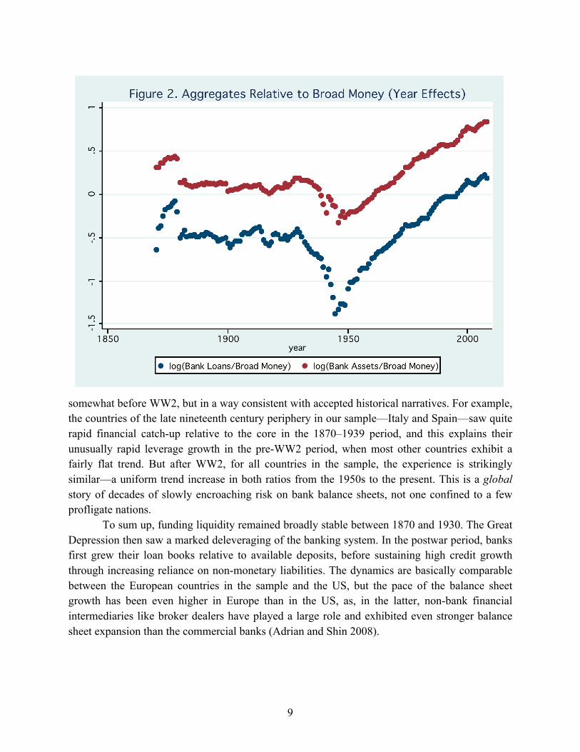
The first important fact that emerges from the data is the presence of two distinct “eras of finance capitalism” as shown in figures 1 and 2. Figure 1 displays the trend in credit and money aggregates relative GDP, while figure 2 displays the long-run trends in the credit to money ratios, where in each case we show the average trend for the 14 countries in our dataset. To construct these average global trends, both here and in some other figures that follow, we show the mean of the predicted time effects from fixed country-and-year effects regressions for the dependent variable of interest. That is for any variable Xit we estimate the fixed effects regression Xit=ai +bt + eit and then plot the estimated year effects bt to show the average global level of X in year t.

From these figures we see that the first financial era lasted from 1870 to World War Two. In this era, money and credit were volatile but over the long run they maintained a roughly stable relationship to each other and relative to the size of the economy as measured by GDP. Money and credit grew just a little faster than GDP in the first few decades of the classical gold standard era from 1870 to about 1890, but then remained more or less stable relative to GDP until the credit boom of the 1920s and the Great Depression. In the 1930s, both money and credit aggregates collapsed. Figure 2 shows that the relationship between then loan or asset measures and broad money remained almost perfectly stable throughout the first era up to WW2, save for the 1930s global credit crunch. In that epoch, money growth and credit growth were essentially two sides of the same coin. The same was not true in the second era after WW2, when loans and assets both embarked on a long, strong secular uptrend relative to broad money, and here both graphs reveal profound structural shifts in the relationship between credit, money, and output.

Thus, during the first era of finance capitalism, up to 1939, the era studied by canonical monetarists like Friedman and Schwartz, the “money view” of the world looks entirely reasonable. Banks’ liabilities were first and foremost monetary, and exhibited a fairly stable relationship to total credit. In that environment, by steering aggregate liabilities of the banking sector, the central bank could hope to exert a smooth and steady influence over aggregate lending.

8

The relationships changed dramatically in the post-1945 period. First, credit began a long recovery after the dual shocks to the financial sector from the Great Depression and the war. Loans and bank assets took off on a very rapid upward trend in the Bretton Woods era as seen in Figure 1, and they managed to surpass their pre-1940 ratios, compared to GDP, by about 1970. Second, credit not only grew strongly relative to GDP, but also relative to broad money after WW2, via a combination of higher leverage and (after the 1970s) through the use of new sources of funding, mainly debt securities, creating more and more non-monetary bank liabilities.4 Again, the pre-WW2 ratios of credit and assets to money were surpassed circa 1970, as seen in Figure 2. Loan-money and asset-money ratios, shown here in logs, continued ever higher, attaining levels +0.750 log points higher than their prewar average by around 2000 (i.e., about ×2 in levels).

We should also note that this structural increase in the credit to money ratio does not only apply to a few individual countries, such as the usual Anglo-Saxon suspects, but has been a common phenomenon across many countries. Figure 3 shows the log loan-money and log asset-money ratios for all 14 countries at benchmark decadal dates. Country experiences vary

4 It is even likely that our numbers underestimate the process of credit creation in the past decades as a growing portion of lending, at least in some countries, was securitized and is no longer carried on bank’s balance sheets.

9

somewhat before WW2, but in a way consistent with accepted historical narratives. For example, the countries of the late nineteenth century periphery in our sample—Italy and Spain—saw quite rapid financial catch-up relative to the core in the 1870–1939 period, and this explains their unusually rapid leverage growth in the pre-WW2 period, when most other countries exhibit a fairly flat trend. But after WW2, for all countries in the sample, the experience is strikingly similar—a uniform trend increase in both ratios from the 1950s to the present. This is a global story of decades of slowly encroaching risk on bank balance sheets, not one confined to a few profligate nations.

To sum up, funding liquidity remained broadly stable between 1870 and 1930. The Great Depression then saw a marked deleveraging of the banking system. In the postwar period, banks first grew their loan books relative to available deposits, before sustaining high credit growth through increasing reliance on non-monetary liabilities. The dynamics are basically comparable between the European countries in the sample and the US, but the pace of the balance sheet growth has been even higher in Europe than in the US, as, in the latter, non-bank financial intermediaries like broker dealers have played a large role and exhibited even stronger balance sheet expansion than the commercial banks (Adrian and Shin 2008).

10

What does this structural change mean for the questions about money, credit and output raised before? First, in the latest phase in which banks fund loan growth through non-monetary liabilities the traditional monetarist view looks unpromising and incomplete. The link between money and credit is now considerably looser than in a model where banks’ liabilities are predominantly or even exclusively monetary. This is exactly what many of the world’s central banks found out in the 1980s, as Friedman and Kuttner (1992) have documented.

Second, if we take the ratio of bank credit to non-monetary liabilities as an indicator of funding leverage, it is easy to see how leverage levels have increased in a historically

11

unprecedented way. Yet this also means that banks’ access to non-monetary sources of finance has become an important factor for aggregate credit provision. Thus, what happens in financial markets—borrowing conditions, liquidity, market confidence—starts to matter more than ever for credit creation and financial stability, possibly amplifying the cyclicality of financing in a major way (Adrian and Shin 2008). The consequences for macroeconomic stability are powerful, since the conventional transmission mechanisms can now be buffeted by large financial shocks. Last but not least, the increasing dependence of the banking system on access to funding from financial markets could also mean that central banks are forced to underwrite the entire funding market in times of distress in order to avoid the collapse of the banking system as witnessed in 2008–09. This “mission creep” follows from the fact that banking stability can no longer rest on the foundations of deposit insurance alone, with the Lender of Last Resort now having to confront wholesale (i.e., nondeposit) bank runs.

To conclude this examination of long-run trends, by taking a closer look at our data we found that one other factor has also contributed to financial fragility in the long run, in addition to the leverage trends documented above. If we now turn away from banks’ liabilities, and look to the composition of the asset side of the balance sheet, we discover another trend that has contributed to increased leverage and risk, namely the shrinkage in liquid safe assets—the kind of assets that might serve as a buffer in times of stress.

To show this trend, Figure 4 displays the mean year effects of the log of the share of securities on balance sheets as well as the log share of government securities. (Note that our data on these detailed balance sheet components start only in 1945). The data show that the overall share of securities on banks’ balance sheets has risen only very slowly over time, and has been stable since 1945. The prewar rise is indicative of financial developments where banks diversify away from pure loan provision and become more like any other type of nonbank asset manager, either in response to innovation, new profit opportunities, or deregulation. But what is more important, as we can see, is that the securities that banks held have become riskier over time. Banks across the sample have sharply reduced their holdings of government securities in the postwar period, from levels that were relatively high at the end of WW2. By 2005 the average share of government securities had fallen by more than 80% (–1.500 log points) compared to the levels seen in the 1950s, and by more than one half (–1.000 log points) even compared to 1970s. Balance sheets have not only became much bigger, financed by wholesale borrowing, their composition has also changed markedly. Banks collectively moved out on the risk curve to buy proportionally more securities from the private sector.

Another way to put it is that banks have progressively diluted their capacity to self-insure through precautionary savings parked in safe, liquid, low-yield assets. This hitherto unknown historical backdrop buttresses arguments that without stronger forms of “capital insurance” or liquidity hoarding requirements, modern banking systems will be prone to skate on the thinnest of ice (Kashyap, Rajan, and Stein 2008; Farhi and Tirole 2009). Indeed, these developments

12

correlate broadly with the frequency of banking crises. The frequency of banking crises in the 1945–71 period was virtually zero, when such liquidity hoards were relatively ample and leverage was low; but since 1971, as these hoards evaporated and banks levered up, crises became much more frequent, with a roughly 4% annual probability.5

5. Money, Credit, and Output after Financial Crises: An Event Analysis In this section we look at financial crises in more depth. We are able to demonstrate the dramatically different crisis dynamics in the two eras of finance capitalism, or now versus then. We exploit our long-run dataset with an eye on improving our understanding of the behavior of money and credit aggregates as well as the responses of the real economy and prices in financial crisis windows before and after WW2. We were concerned that our results might be strongly influenced by the Great Depression, so we also re-ran our analysis excluding data for the 1930s Depression window, but we obtained similar results as documented below. We find substantially different dynamics in the pre and post WW2 periods which we think reflect different monetary

5 Frequency of banking crises from Bordo et al. (2001, Figure 1).

13

and regulatory frameworks: the shift away from gold to fiat money, the greater role of activist macroeconomic policies, and greater emphasis on bank supervision and deposit insurance.

For the event-analysis we adopt an annual coding of financial crisis episodes based on documentary descriptions in Bordo et al. (2001) and Reinhart and Rogoff (2009), two widely-used historical data sets that we compared and merged for a consistent definition of event windows (a table showing the crisis events can be found in the appendix). We have also corroborated these crisis histories with alternative codings found in the databases compiled by Laeven and Valencia (2008), as well the evidence described in Cecchetti et al. (2009). In line with the previous studies we define financial crises as events during which a country’s banking sector experiences bank runs, sharp increases in default rates accompanied by large losses of capital that result in public intervention, bankruptcy, or forced merger of financial institutions.

Figure 5a opens the discussion with a look at the behaviour of money and credit in the aftermath of financial crises. We see that there are clear differences between the two eras of finance capitalism. Before WW2, credit and money growth dipped significantly below normal levels after crisis events and did not recover to pre-crisis growth rates until fully five years after the crisis. In contrast, after WW2 a dip in the growth rate of the monetary and credit aggregates

14

is hardly discernible in the aftermath of a crisis.6 We infer that in the later period, central banks have supported growth of the monetary base, prevented collapse of broad money, and thus kept bank lending at comparatively high levels. Only total bank assets now behave in a meaningfully different way after financial crises, as we will discuss in further detail below.

Turning to real economic effects shown in Figure 5b, it becomes clear that the impact of financial crises was more muted in the postwar era in absolute numbers, but of comparable magnitude relative to trend. As mentioned before, this result holds up even when the Great Depression is excluded from the prewar event analysis. Measured by output declines, financial crises remain severe in the post-1945 period. The maximum decline in real investment activity was somewhat more pronounced before WW2, albeit with a sharp bounce back after 4 to 5 years.

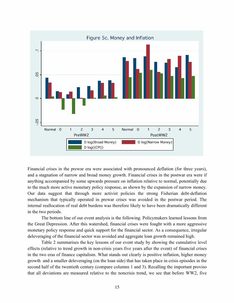
Turning to Figure 5c, we see that it is with regard to price developments that a major difference between the two eras appears, which is again not driven by the Great Depression.

6 It is sometimes claimed that negative credit growth would be a signal of a credit crisis (e.g. Chari et al. 2008). In our data, before WW2 crises were associated with slightly negative average loan growth in the year after the crisis began. However, this result is influenced by the Great Depression. In general it is the second derivative of loan growth that changes sign during a crisis, not the first. See Biggs et al. (2009) for an explanation and related evidence.

15

Financial crises in the prewar era were associated with pronounced deflation (for three years), and a stagnation of narrow and broad money growth. Financial crises in the postwar era were if anything accompanied by some upwards pressure on inflation relative to normal, potentially due to the much more active monetary policy response, as shown by the expansion of narrow money. Our data suggest that through more activist policies the strong Fisherian debt-deflation mechanism that typically operated in prewar crises was avoided in the postwar period. The internal reallocation of real debt burdens was therefore likely to have been dramatically different in the two periods.

The bottom line of our event analysis is the following. Policymakers learned lessons from the Great Depression. After this watershed, financial crises were fought with a more aggressive monetary policy response and quick support for the financial sector. As a consequence, irregular deleveraging of the financial sector was avoided and aggregate loan growth remained high.

Table 2 summarises the key lessons of our event study by showing the cumulative level effects (relative to trend growth in non-crisis years five years after the event) of financial crises in the two eras of finance capitalism. What stands out clearly is positive inflation, higher money growth and a smaller deleveraging (on the loan side) that has taken place in crisis episodes in the second half of the twentieth century (compare columns 1 and 3). Recalling the important proviso that all deviations are measured relative to the noncrisis trend, we see that before WW2, five

16

years after a crisis year the level of broad money was 14 percent below trend, and bank loans 24 percent below trend. In the postwar period, however, the declines were a mere 6 percent (not statistically significant) for broad money and 15 percent for bank loans. However, in the mirror of our data the effect on the securities side of banks’ balance sheets in response to financial crisis is even stronger, with bank assets falling 24 percent below trend in the postwar period, versus 11 percent prewar. This clearly confirms the modern findings by Adrian and Shin (2008) who argue that the behaviour of non-loan items on the balance sheets of financial institutions is particularly procyclical.

Turning to real effects, it is interesting to observe that despite the much more aggressive policy response in the postwar period, the cumulative real effects have been even somewhat stronger in the postwar period. In the aftermath of postwar financial crises output dropped a cumulative 6.2 percent relative to trend, and real investment by more 22 percent. The prewar output decline effect, however, is largely an artefact of the massive financial implosions of the 1930s. Excluding the 1930s (see column 2), the cumulative real output and investment declines after crises were substantially smaller and not statistically significant. The finding of limited losses prior to the 1930s would be consistent with the idea that in the earlier decades of our sample the financial sectors played a less central role in the economy and financial crises were hence less costly. It is also consistent with the view that economies suffered less from nominal rigidity, especially before 1913, as compared to the 1930s, and hence were better able to adjust to nominal shocks like crisis-induced debt-deflation (Chernyshoff et al. 2009).

Why are output losses so large today despite more activist policies? Some other forces might be at work here. Governments have made more efforts since the 1930s to prevent negative feedback loops in the economy and have sought to cushion the real and nominal impact of financial crises through policy activism. But at the same time the financial sector has grown and

TABLE 2 CUMULATIVE EFFECTS AFTER FINANCIAL CRISES Cumulative log level effect, after years 0–5 of crisis, versus noncrisis trend, for:

Pre–World War 2 Pre–World War 2, excluding 1930s

Post–World War 2

Log broad money –0.141*** (0.027)

–0.103*** (0.029)

–0.062 (0.039)

Log bank loans –0.236*** (0.044)

–0.179*** (0.048)

–0.148*** (0.053)

Log bank assets –0.113*** (0.034)

–0.078** (0.037)

–0.239*** (0.048)

Log real GDP –0.045** (0.020)

–0.018 (0.020)

–0.062*** (0.017)

Log real investment –0.203** (0.094)

–0.114 (0.093)

–0.222*** (0.047)

Log price level –0.084*** (0.025)

–0.047* (0.027)

+0.009 (0.028)

Notes: *** denotes significance at the 99% level, ** 95% level, and * 90% level. Standard errors in parentheses.

17

increased leverage, expanding the size of the threat even as the policy defences have been strengthened. As a result the shocks hitting the financial sector might now have a potentially larger impact on the real economy, absent the policy response. Still, a complete diagnosis has to recognize the potential reverse causality too: it is an open question to what extent implicit government insurance and the prospect of rescue operations have in turn contributed to the spectacular growth of finance and leverage within the system, creating more of the very hazards they were intending to solve.

6. Credit Booms and Financial Crises

In the previous sections we have documented the rise of credit and discussed how activist monetary policy responses to crises could have been a factor behind the uninterrupted growth of leverage in the postwar financial system. We now look at the sources of recurrent financial instability in modern economies. More specifically, we want to know whether the financial system itself creates economic instability through endogenous lending booms. In other words, are financial crises “credit booms gone wrong”?

By looking at the role of the credit system as a potential source of financial instability—and not merely as an amplifier of shocks as the financial accelerator theory has it—we implicitly also ask a different question about the importance of credit in the conduct of monetary policy. The pre-crisis New Keynesian consensus held that money and credit have essentially no constructive role to play in monetary policy. Hence, central bankers were to set interest rates in response to inflation and the output gap, with no meaningful additional information coming from credit or monetary aggregates. Yet even before the crisis of 2008/09 this view did not go unchallenged. A number of dissenters argued that money and credit aggregates provided valuable information for policymakers aiming for financial and economic stability.7 On this point, one could also detect echoes of other recent research pointing to a tentative relationship between credit booms and financial fragility in studies of emerging market crises.8 The idea that financial crises are credit booms gone wrong is not new. The story underlies the oft-cited works of Minsky (1977) and Kindleberger (1978), and it has been put forward as a factor in the current cycle (Hume and Sentance 2009; Reinhart and Rogoff 2009) as well as in the Great Depression (Eichengreen and Mitchener 2003). Yet statistical evidence is still scant. Although the explanation appears as a robust element in descriptions of emerging market crises (e.g., McKinnon and Pill 1997; Kaminsky and Reinhart 1999), evidence that the same problem afflicts advanced countries has not yet attained a consensus position—partly due to the small

7 Some argued that excessive credit created “imbalances” and a risk of financial instability (e.g., Borio and Lowe 2002, 2003; White 2004; Goodhart 2007). Recent theories show how a credit signal might dampen suboptimal business-cycle volatility (Christiano, Motto, and Rostagno 2007). 8 On the whole, the early-warning literature on banking crises focuses mainly on (i) emerging markets and (ii) factors other than lending booms (for a survey see Eichengreen and Arteta, 2002 Table 3.1). Exceptions, which use data from recent decades only, include Demirgüç-Kunt and Detragiache (1998); Kaminsky and Reinhart (1999); Gourinchas, Valdes, and Landerretche (2001). Particularly relevant works are those by Borio and Lowe (2002, 2003), who like us focus on cumulative effects and place a high weight on the lagged credit growth signal.

18

sample sizes provided by recent history. Moving beyond explorations of selected events, our interest is in whether there is systematic evidence for this mechanism in history. If we can find such a link, then the argument for the credit boom-and-bust story will be strengthened. To test for this link we propose to use a basic forecasting framework to ask a simple question: does a country’s recent history of credit growth help predict a financial crisis, and is this robust to different specifications, samples, and control variables? Formally, we use our long-run annual data for 12 countries, and estimate a probabilistic model of a financial crisis event in country i, in year t, as a function of a lagged information at year t, in one of two forms,

OLS Linear Probability: pit = b0i + b1(L) D log CREDITit + b2(L) Xit + eit , Logit: logit(pit) = b0i + b1(L) D log CREDITit + b2(L) Xit + eit ,

where logit(p)=ln(p/(1–p)) is the log of the odds ratio and L is the lag operator. The CREDIT variable will usually be defined as our total bank loans variable deflated by the CPI. The lag polynominal b1(L), which contains only lag orders greater than or equal to 1, will be the main object of study and the goal will be to investigate whether the lags of credit growth are informative. The lag polynominal b2(L) will, if present, allow us to control for other possible causal factors in the form of additional variables in the vector X. The error term eit is assumed to be well behaved. We first present some simple variants of these models in Table 3. These results take the form of an estimate of the above equations with no additional controls, so that the term X is omitted. In this long and narrow panel there are 1285 observations over 14 countries, with an average of about 93 observations per country. The dependent variable is a dummy equal to one when there is a banking crisis according to our definitions, and otherwise zero. Our crisis definitions are the same as detailed above.

To keep the lag structure reasonable, we consider up to five annual lags of any regressor.9 Model specification 1 presents an OLS Linear Probability model with simple pooled data. Model specification 2 adds country fixed effects to the OLS model, but these are not statistically significant (p=0.85). Keeping country effects, model specification 3 then adds year effects to OLS, and these are highly statistically significant. What does this say? It implies that there is a common global time component driving financial crises—and, if you happen to know ex ante this effect, you can use it to dramatically enhance your ability to predict crises. This is not too surprising given the consensus view that financial crises have tended to happen in waves and often afflict multiple countries, but is also not of very much practical import for out-of-sample forecasting, since such time effects are not known ex ante. Thus, from now on, given our focus on prediction, we study only models without time effects.

9 Formal lag selection procedures (AIC, BIC, and likelihood ratio tests) suggest we could in most cases use just two lags of CREDIT; however higher order lags are sometimes significant, as can be seen in Table 2, and credit booms are typically considered phenomena that last for many years, so we maintain 5 lags as our initial specification.

19

In all of the OLS models the sum of the lag coefficients is about 0.36, which is easy to interpret. Average real loan growth over 5 years in this sample has a standard deviation of about 0.07, so a one standard deviation change in real loan growth increases the probability of a crisis by 0.0252 or 2.5 percentage points. Since the sample frequency of crises is just under 4 percent, this shows a high sensitivity of crises to plausible shocks within the empirical range of observed loan growth disturbances. Still, there are well known problems with the Linear Probability model, notably the fact that the domain of its fitted values is not constrained to the unit interval relevant for a probability outcome. Thus in columns 4 and 5 we switch to a Logit model. Model specification 4 displays pooled Logit, and specification 5 adds country fixed effects by including dummies in the regression, though again these are not statistically significant. Unfortunately, we cannot implement a Logit model with year effects. In our setting, the problem is small N and large T, the

TABLE 3 FINANCIAL CRISIS PREDICTION—OLS AND LOGIT ESTIMATES (1) (2) (3) (4) (5) Baseline Estimation method OLS OLS OLS Logit Logit Fixed effects None Country Country+year None Country L.Dlog(loans/P) -0.0182 -0.0144 -0.0218 -0.0917 -0.108 (0.077) (0.077) (0.079) (1.93) (2.05) L2.Dlog(loans/P) 0.260*** 0.265*** 0.273*** 6.641*** 7.215*** (0.082) (0.083) (0.083) (1.68) (1.99) L3.Dlog(loans/P) 0.0638 0.0678 0.0445 1.675 1.785 (0.081) (0.081) (0.081) (1.67) (1.83) L4.Dlog(loans/P) -0.00423 -0.00329 0.0357 0.0881 0.0517 (0.077) (0.077) (0.078) (1.38) (1.49) L5.Dlog(loans/P) 0.0443 0.0464 0.0712 0.998 1.073 (0.071) (0.071) (0.072) (1.73) (1.78) Observations 1285 1285 1285 1285 1285 Groups 14 14 14 14 14 Avg. obs. per group 91.79 91.79 91.79 91.79 91.79 Sum of lag coefficients 0.345*** 0.361*** 0.403*** 9.311*** 10.02*** se 0.116 0.119 0.0093 2.812 0.0388 Test for all lags = 0† 3.26*** 3.36*** 3.18*** 21.92** 17.22** p value 0.0063 0.0051 0.0075 0.0005 0.0041 Test for country effects = 0† — 0.62 0.69 — 7.79 p value — 0.8381 0.7759 — 0.8571 Test for year effects = 0† — — 2.87*** — — p value — — 0.0000 — — R2† 0.0126 0.0188 0.2197 0.0379 0.0596 Pseudolikelihood — — — -197.12 -192.67 Overall test statistic†† 3.26*** 1.35 2.91*** 21.92*** 33.07** p value 0.063 0.1475 0.0000 0.0005 0.0164 Predictive ability, AUROC 0.659*** 0.698*** 0.943*** 0.659*** 0.697*** se 0.0373 0.0380 0.0093 0.0374 0.0388 Notes: *** p<0.01, ** p<0.05, * p<0.1. † Reported statistic is Pseudo R2 for Logit. †† Reported statistic is F for OLS, χ2 for logit. Standard errors in parentheses. Logit standard errors are robust.

20

opposite of typical microeconometric applications. This means that the incidental parameters problem afflicts the T dimension, and we have consistency in N. Conditional fixed effects can only be estimated using years in the panel where there is actual variation in the outcome variable. In our case, this collapses the number of observations from 1285 to just 140, so that model parameters could not be precisely estimated. We accordingly adopt Column 5, the Logit model with country effects but without time-effects, as our preferred baseline specification henceforth. Our key finding is that all forms of the model show that a credit boom over the previous five years is indicative of a heightened risk of a financial crisis. The diagnostic tests reported show that the five lags are jointly statistically significant at the conventional 5% level; the regression chi-squared is also significant. The difference between the first and second lag coefficients is also suggestive; the former is negative and the latter large and positive, confirming that when the second derivative of credit changes sign we can see that trouble is likely to follow (Biggs, Meyer, and Pick 2009). The sum of the lag coefficients is about 8.8, and also statistically significant. To interpret this we need to convert to marginal effects, where in Column 5, at the means of all variables, the sum of the marginal effects over all lags is 0.285, similar, albeit a little smaller, than the 0.36 estimate given by the OLS Linear Probability model noted above.

Finally we note that in all its forms the model has predictive power, as judged by a standard tool used to evaluate binary classification ability, the Receiver Operating Characteristic (ROC) curve. This is shown in Figure 6 for our preferred baseline model. The curve plots the true positive rate TP(c) against the false positive rate FP(c), for all thresholds c on the real line, where the binary classifier is , I(.) is the indicator function, and is the linear prediction of the model which forms a continuous signal. When the threshold c gets large and negative, the classifier is very aggressive in making crisis calls, almost all signals are above the threshold, and TP and FP converge to 1; conversely, when c gets large and positive, the classifier is very conservative in making crisis calls, almost all signals are below the threshold, and TP and converge to 0. In between, an informative classifier should deliver TP > FP so the ROC curve should be above the 45-degree line of the null, uninformative (or “coin toss”) classifier. At this point we would prefer not to take a stand on where the policy maker would place the cutoff value of the threshold. The utility computation depends on costs of different outcomes and the frequency of crises. For example, the cutoff should be more aggressive if the cost of an undiagnosed crisis is high, but less so if the cost of a false alarm is higher. If crises are rare, the threshold bar should also be raised to deflect too-frequent false alarms (see Pepe 2003). Fortunately, a test of predictive ability exists that is independent of the policymaker’s cutoff. This is the area under the ROC curve (AUROC). It is essentially a test of whether the distribution of the model’s signals are significantly different under crisis and noncrisis states, thus allowing them to used a basis for meaningfully classifying these outcomes. The AUROC provides a simple test against the null value of 0.5 with an asymptotic normal distribution, and for our baseline model AUROC=0.697 with a standard error of just 0.039. The model can therefore be

21

judged to have predictive power versus a coin toss, although it is far from a perfect classifier which would have AUROC = 1.10

All the above forecasts suffer from in-sample look-ahead bias, even though they use lagged data. To put our model to a sterner test, we limited the forecast sample to the post-1983 period only (325 country-year observations) and compared in-sample and out-of-sample forecasts (the former based on full sample predictions, with look-ahead bias; the latter based on rolling regressions, using lagged data only). The in-sample forecast produced an even higher AUROC=0.787 (s.e. = 0.061), but the out-of-sample also proved informative, with an AUROC=0.674 (s.e. = 0.073), with the latter having statistical significance at better than the 5% level. We think any predictive power is impressive at this stage given the general skepticism evinced by the “early warning” literature, and our out-of-sample results add some reassurance. We now ask some questions about the value added of our results and their robustness. The first claim we make is that the use of credit aggregates, rather than monetary aggregates, is of crucial importance. This would have broad implications, first for economic history, since monetary aggregates have been widely collected and may be easily put to use. But it also has 10 Is 0.7 a “high” AUROC? For comparison, in the medical field where ROCs are widely used for binary classification, an informal survey of newly published prostate cancer diagnostic tests finds AUROCs of about 0.75.

22

policy implications. Indeed, after the crisis of 2008–09 the argument has often been heard that greater attention to such aggregates, in contrast to a narrow focus on the Taylor rule indicators of output and inflation, might have averted the crisis. But when we look at the long run data systematically, monetary aggregates are not that useful as predictive tools in forecasting crises, in contrast to the correct measure, total credit. We find the success of the credit measure appealing, and not just because it vindicates the drudgery of our laborious data collection efforts: we think credit is a superior predictor, because it better captures important, time-varying features of bank balance sheets such as leverage and non-monetary liabilities. The basis for these claims is the collection of results reported in Tables 4 and 5. In Table 4 we start with the baseline model, reproduced in model specification 6. All through this table we continue to estimate the model over the entire sample, using the Logit model with country fixed effects. Having settled on this model, we now also report, for completeness, the marginal effects on the predicted probability evaluated at the means for the lags of credit. We then take several perturbations of the baseline that take the form of replacing the five lags of the credit variable with alternative measures of money and credit.

Specification 7 replaces real loans with real broad money, still deflated by CPI. The fit is still statistically significant, although slightly weaker judging from lower R2, pseudolikelihood, and significance levels on the lags. In terms of predictive power, the AUROC is also marginally lower. However, the basic message at this point is that broad money could potentially proxy for credit. Both the liability and the asset side of banks’ balance sheets seem to do a good job at predicting financial trouble ahead over the whole sample—though we shall qualify this result in a moment. Specification 8 replaces loans with narrow money and the model falls apart, which is not unexpected; given the instability in the money multiplier, the disconnect between base money and credit conditions is too great to expect this model to succeed. Specifications 9 and 10 replace real loans with the loans-to-GDP ratio and the loans-to-broad-money ratio, respectively. Both of these variants of the model also meet with some success, and specification 9 outperforms slightly in terms of measures of fit and predictive ability as measured by AUROC.

So far the main results might tempt us to conjecture, first, that various scalings of credit volume could have similar power to predict financial crises; and, second, that broad money could also proxy for credit adequately well. The former idea may be true, but Table 5 quickly dispels the latter. The robustness checks here take the form of splitting the sample into pre-WW2 and post-WW2 samples, where we are guided to conduct this test by the summary findings above showing very different trends in the behavior of money and credit in these two epochs.

Specifications 11 and 12 show that using our credit measure, real loans, the baseline model performs quite well in terms of both fit and predictive power both before and after WW2. Column 12 is particularly interesting, since the significant and alternating signs of the first and second lag coefficients in the postwar period highlight the sign of the second derivative (not the first) in raising the risk of a crisis. In contrast, specifications 13 and 14 expose some unsatisfactory performance when broad money is used. Before WW2 the weaknesses are not evident, with the lags of broad money still significant, and similar predictive power. But after

23

WW2 the model based on broad money is a failure: the fit is much poorer, and from a predictive standpoint the model has a much lower AUROC.

To explore the predictive ability differences more closely using ROC tools, we examined the four ROC curves shown Figure 7, this time computed on common samples within each period (thus the statistics differ slightly from those seen in Table 6). We then used AUROC comparison tests along with Kolmogorov-Smirnov tests (of the difference in the signal distributions under each outcome) to see whether one model or the other was to be preferred in each period for its binary classification ability.

TABLE 4 BASELINE MODEL AND ALTERNATIVE MEASURES OF MONEY AND CREDIT (6) (7) (8) (9) (10) Specification Baseline Replace Replace Replace Replace (Logit country effects) loans with loans with real loans real loans broad narrow with loans/ with loans/

money money GDP broad money

L.Dlog(loans/P) -0.108 1.942 -0.890 1.224 -0.447 (2.05) (2.94) (1.37) (2.19) (1.92) L2.Dlog(loans/P) 7.215*** 5.329** 2.697 7.975*** 7.244*** (1.99) (2.52) (1.68) (1.96) (2.08) L3.Dlog(loans/P) 1.785 2.423 2.463 4.525** 0.767 (1.83) (2.63) (1.77) (1.86) (2.19) L4.Dlog(loans/P) 0.0517 -1.742 -2.244 1.874 2.620 (1.49) (2.51) (1.65) (1.44) (1.98) L5.Dlog(loans/P) 1.073 4.275* 1.210 2.276 -1.386 (1.78) (2.30) (1.82) (1.69) (2.63) Marginal effects -0.003 0.060 -0.029 0.032 -0.014 at each lag 0.205 0.165 0.088 0.210 0.222 evaluated at the means 0.051 0.075 0.080 0.119 0.024 0.001 -0.054 -0.073 0.050 0.080 0.031 0.132 0.039 0.060 -0.043 Sum 0.285 0.378 0.105 0.472 0.270 Observations 1285 1361 1394 1258 1237 Groups 14 14 14 14 14 Avg. obs. per group 91.79 97.21 99.57 89.86 88.36 Sum of lag coefficients 10.02*** 12.23*** 3.235 17.87*** 8.798* se 3.235 3.544 3.129 3.899 4.607 Test for all lags = 0, χ2 17.22*** 18.35*** 5.705 25.16*** 13.25** p value 0.0041 0.0025 0.3360 0.0001 0.0211 Test for country effects = 0, χ2 7.789 9.333 8.627 7.302 8.595 p value 0.857 0.747 0.800 0.886 0.803 Pseudo R2 0.0596 0.0481 0.0343 0.0852 0.0493 Pseudolikelihood -192.7 -213.2 -220.7 -186.5 -193.0 Overall test statistic, χ2 33.07** 36.45*** 14.88 43.70*** 28.27* p value 0.0164 0.0061 0.670 0.000638 0.0580 Predictive ability, AUROC 0.697*** 0.689*** 0.629*** 0.728*** 0.695*** se 0.0388 0.0332 0.0382 0.0369 0.0365 Notes: *** p<0.01, ** p<0.05, * p<0.1. Robust standard errors in parentheses.

24

Before WW2 (for N=465 common observations) a test of equality in AUROCs between the credit and money models passed easily (p = 0.84); the ROC curves are very close to each other and almost overlapping; and both models attain a maximum height above the diagonal that is significantly different from zero. After WW2 (for N = 768 common observations) the money model ROC curve is below the credit model ROC curve at almost all points, except at a few points close to the (0,0) and (1,1) points, where operation is unlikely to be optimal for the policymaker; the two AUROCs are different, with a p-value quite near to the 10% level (p =

TABLE 5 BASELINE MODEL WITH PRE-WW2 AND POST WW-2 SAMPLES

(11) (12) (13) (14)

Specification Baseline Baseline Pre WW2 sample

Post WW2 sample

(Logit country effects)

Pre WW2 sample

Post WW2 sample

replace loans with

replace loans with

using loans using loans broad money broad money L.Dlog(loans/P) 2.898 -2.574 3.521 0.692 (2.61) (3.53) (3.31) (5.01) L2.Dlog(loans/P) 6.461*** 10.06*** 6.681* 3.809 (2.42) (2.94) (3.47) (2.55) L3.Dlog(loans/P) 3.257 1.985 2.151 4.170** (2.22) (2.75) (3.06) (2.09) L4.Dlog(loans/P) 0.949 1.760 -0.841 0.0627 (1.63) (2.63) (2.24) (4.98) L5.Dlog(loans/P) 3.073 -2.354 5.846** 0.860 (1.91) (3.16) (2.92) (3.87) Marginal effects 0.108 -0.0484 0.141 0.0156 at each lag 0.241 0.189 0.267 0.0857 evaluated at the means 0.122 0.0373 0.0861 0.0938 0.035 0.0331 -0.0337 0.00141 0.115 -0.0442 0.234 0.0193 Sum 0.621 0.167 0.695 0.216 Observations 488 775 563 776 Groups 13 14 13 14 Avg. obs. per group 37.54 55.36 43.31 55.43 Sum of lag coefficients 16.64*** 8.876 17.36*** 9.595* se 5.263 5.755 6.019 5.624 Test for all lags = 0, χ2 12.68** 14.04** 13.92** 9.318* p value 0.0266 0.0153 0.0161 0.0970 Test for country effects = 0, χ2 4.036 5.644 9.726 6.183 p value 0.983 0.958 0.640 0.939 Pseudo R2 0.0933 0.0851 0.0878 0.0408 Pseudolikelihood -94.65 -88.28 -112.0 -92.57 Overall test statistic, χ2 26.09* 59.95*** 39.55*** 17.52 p value 0.0729 0.0000 0.0015 0.4880 Predictive ability, AUROC 0.717*** 0.736** 0.742*** 0.655*** se 0.0445 0.0623 0.0379 0.0581 Notes: *** p<0.01, ** p<0.05, * p<0.1. Robust standard errors in parentheses. In the prewar sample NLD is dropped from the logit regression because there are no crises in the sample (with five lags of credit or money in non-war years), so N=13 for these cases.

25

0.16). We also find that of the four ROCs in Figure 7, only the Post-WW2 money model fails the Kolmogorov-Smirnov test, so its maximal height above the diagonal (TP minus FP) is not statistically different from zero at conventional levels, which is also highly discouraging.

How do we interpret these results? The findings mesh well with our overall understanding of the dramatic changes in money and credit dynamics after the Great Depression. In the summary data for the pre-WW2 sample, we saw how broad money and credit moved hand in hand, so that a Friedman “money view” of the financial system, focusing on the liability side of banks’ balance sheets, was an adequate simplification. After WW2 this was no longer the case, and credit was delinked from broad money aggregates, which would beg the question as to

26

which was the more important aggregate in driving macroeconomic outcomes. At least with respect to crises, the results of our analysis are clear: credit matters, not money.

These findings have potentially important policy implications, especially for central banks that still embrace the oft forgotten idea of using quantitative indicators as a “pillar” of monetary policymaking. If this pillar is there as to support price stability goals, then indeed a monetary aggregate may be the right tool for the job; but if financial stability is a goal, then our results suggest that a better pillar might make use of credit aggregates instead and their superior power in predicting incipient crises.

To underscore the value of our model based on the “credit view”, and to guard against omitted variable bias, in Table 6 we subject our baseline specification to several perturbations that take the form of including additional control variables X as described above. Specifications 15 adds 5 lags of real GDP growth. Specification 16 adds 5 lags of the inflation rate, since inflation has been found to contribute to crises in some studies (e.g., Demirgüç-Kunt and Detragiache 1998). Neither set of controls can raise the fit and predictive performance of the model slightly. However, the inclusion of these terms has little effect on the coefficients on the lags of credit growth, their quantitative or statistical significance, and their substantive contribution to the model’s predictive ability. Specifications 17 and 18 add 5 lags of the nominal short-term interest rate or its real counterpart, since some studies find that high interest rates, e.g. to defend a peg, can help trigger crises (e.g., Kaminsky and Reinhart 1999); only the lags of the real interest rate are just significant at the 5% level, but they do not alter the baseline story and the credit effects remain strong. Finally, in specification 19 we add 5 lags of the change in the investment-to-GDP ratio, to explore the possibility that the nature of the credit boom might affect the probability that it ends in a crisis. For example, according to arguments heard from time to time, if credit is funding “productive investments” then the chances that something can go wrong are reduced—as compared to credit booms that fuel consumption binges or feed speculative excess by households, firms, and/or banks.11 Our results caution against this rosy view. Over the long run, in our developed country sample, most of the lags of investment are not statistically significant at the conventional level, and the only one that is actually has a “wrong” positive sign, suggesting that crises are slightly more likely when they have been funding investment booms as opposed to other activity.12 If this is the case, then the suspicion arises that when banks originate lending, they may be almost equally incapable of assessing repayment capacity in all cases, with investment loans having no special virtues, and possibly some vices.

11 The argument has often been applied to foreign capital flows manifest in current account deficits. The argument that capital flowing into investment booms does not matter has been variously stated as the “Lawson doctrine,” “Pitchford critique,” or “consenting adults view.” See Edwards (2000) for a survey of this area. 12 The sum of the lags on investment is positive, so crises are marginally more likely in an investment boom, controlling for credit growth.

27

Summing up the results from Table 6, we conjecture that, although some of the auxiliary control variables may matter in some contexts—perhaps in other samples that include emerging markets—for the developed economies these other factors are not the main signal of financial instability problems. Rather the key indicator of a problem is an excessive credit boom. Indeed, the sum of the lag loan coefficients (or their marginal effects) is even higher in Table 6 columns (15)–(19) than in the baseline specification (6), so credit effects are amplified here, rather than being diminished by the added controls; and the Pseudo R2 values range between 0.0833 and

TABLE 6 MORE ROBUSTNESS CHECKS

(15) (16) (17) (18) (19) Specification Baseline Baseline Baseline Baseline Baseline (Logit country effects) plus plus plus plus plus 5 lags of 5 lags of 5 lags of 5 lags of 5 lags of real GDP inflation nominal real change in growth s.t. int. rate s.t. int. rate I/Y L.Dlog(loans/P) 1.192 -0.937 0.735 -1.206 -0.205 (2.19) (2.33) (2.16) (2.61) (2.20) L2.Dlog(loans/P) 8.131*** 10.15*** 8.634*** 10.77*** 7.290*** (1.99) (2.16) (2.22) (2.26) (2.13) L3.Dlog(loans/P) 3.065 0.0626 1.748 0.233 1.214 (1.90) (1.84) (2.17) (2.04) (2.02) L4.Dlog(loans/P) 1.500 1.270 -0.674 1.948 1.357 (1.50) (1.63) (1.87) (1.74) (1.62) L5.Dlog(loans/P) 2.030 -0.157 1.204 -0.378 2.482 (1.67) (2.02) (2.32) (1.97) (2.12) Marginal effects 0.030 -0.024 0.022 -0.035 -0.005 at each lag 0.206 0.256 0.263 0.308 0.187 evaluated at the means 0.078 0.0016 0.053 0.007 0.031 0.038 0.032 -0.021 0.056 0.035 0.051 -0.004 0.037 -0.011 0.064 Sum 0.403 0.262 0.355 0.325 0.312 Observations 1285 1285 1028 1021 1231 Groups 14 14 14 14 14 Avg. obs. per group 91.79 91.79 73.43 72.93 87.93 Sum of lag coefficients 15.92*** 10.39*** 11.65*** 11.37*** 12.14*** se 4.298 3.356 3.650 3.570 3.942 Test for all lags = 0, c2 22.86*** 26.51*** 20.48*** 27.33*** 16.75*** p value 0.0003 0.0000 0.0010 0.0000 0.0050 Test lags of added vbl. = 0, χ2 18.90*** 21.26*** 7.168 15.88*** 10.25* p value 0.0020 0.0007 0.2080 0.0072 0.0683 Test for country effects = 0, χ2 8.106 8.903 10.39 8.763 8.525 p value 0.837 0.780 0.662 0.791 0.808 Pseudo R2 0.0891 0.0943 0.0833 0.1090 0.0896 Pseudolikelihood -186.6 -185.6 -169.4 -164.3 -181.7 Overall test statistic, χ2 43.11*** 57.15*** 50.35*** 55.63*** 47.94*** p value 0.0067 0.0000 0.0008 0.0002 0.0017 Predictive ability, AUROC 0.711*** 0.756*** 0.712*** 0.744*** 0.737*** se 0.0472 0.0424 0.0495 0.0472 0.0494 Notes: *** p<0.01, ** p<0.05, * p<0.1. Robust standard errors in parentheses.

28

0.1090, compared to the 0.0596 value in the baseline case, showing that the greater fraction of the model’s fit is always due to the credit terms.

To conclude, a predictive analysis of our large long-term, cross-country dataset lends support to the idea that, for the most part, financial crises throughout modern history can be viewed as “credit booms gone wrong” (Eichengreen and Mitchener 2003). From our regressions, past growth of credit emerges as the single best predictor of future financial instability, a result which is robust to the inclusion of various other nominal and real variables. Moreover, credit growth seems a better indicator than its nearest rival measure, broad money growth, especially in the postwar period. In light of the structural changes of the financial system that we documented above, this comes as no surprise. As credit growth has increasingly decoupled from money growth, credit and money aggregates are no longer two sides of the same coin. This brings us back to the crucial questions raised at the beginning of this section—should central banks pay attention to credit aggregates or confine themselves to following inflation targeting rules? Historical evidence suggests that credit has a constructive role to play in monetary policy. Valuable information about macroeconomic and financial stability would be missed if policy-makers chose to ignore the behavior of credit aggregates, although how this information is included in the overall policy and regulatory regime is an open and much debated question.

Our results also strengthen the idea that credit matters, above and beyond its role as propagator of shocks hitting the economy. The credit system is not merely an amplifier of economic shocks as in the financial accelerator model of BGG. The importance of past credit growth as a predictor for financial crises and the robustness of the results to the inclusion of other key macro variables, raises the strong possibility that the financial sector is quite capable of creating its very own shocks. In this sense, our historical data vindicate the ideas of scholars such as Minsky (1977) and Kindleberger (1978) who have argued that the financial system itself is prone to generate economic instability through endogenous credit booms.

6. Conclusions Our ancestors lived in an Age of Money, where aggregate credit was closely tied to aggregate money, and formal analysis could use the latter as a reliable proxy for the former. Today, we live in a different world, an Age of Credit, where financial innovation and regulatory ease has permitted the credit system to increasingly delink from monetary aggregates, setting in train an unprecedented expansion in the role of credit in the macroeconomy. Without an adequate historical perspective, these profound changes are difficult to appreciate, and one task of this paper has been to document the nature of this evolution and its ramifications over the last 140 years for a group of major developed economies.

We have shown how the stable relationship between money and credit broke down after the Great Depression and World War 2, as a new secular trend took hold that carried on until today’s crisis. We conjecture that these changes conditioned, and were conditioned by, the broader environment of macroeconomic and financial policies: after the 1930s the ascent of fiat money plus Lenders of Last Resort—and a slow shift back toward financial laissez faire—

29

encouraged the expansion of credit to occur. The policy backstop also, to some degree, insulated the real economy from a scaling up of the damaging effects that prior crises had wrought in days when the financial system played a less pivotal role. However, implicit government insurance and the prospect of rescue operations might also have contributed to the spectacular growth of finance and leverage within the system, creating more of the very hazards they were intending to solve. Aiming to cushion the real economic effects of financial crises, policy-makers have prevented a periodic deleveraging of the financial sector resulting in the virtually uninterrupted growth of leverage we have seen up until 2008. The important structural changes that have taken place in the financial system over the past decades have led to a greater, not smaller role of credit in the macroeconomy. It is mishap of history that just at the time when credit mattered more than ever before, the reigning doctrine had sentenced it to playing no constructive role in monetary policy.

In terms of lessons for policymakers and researchers, history demonstrates that they ignore credit at their peril. The behavior of credit aggregates contains valuable information about the likelihood of future financial crises. It is not, of course, a perfect predictor, and there may be fundamental reasons why, in some periods, especially in eras of financial development and innovation, credit expands to support real economic gains. At the same time, the long-run record shows that recurrent episodes of financial instability have more often than not been the result of credit booms gone wrong, most likely due to failures in the operation and/or regulation of the financial system. For economists, adherence to the money view, not to mention the irrelevance view, has been seriously called into question by the crisis, and the evidence in this paper serves to amplify these doubts amid talk of a “paradigm shift.”13 For policymakers, a complacent attitude towards the growth in the scale and riskiness of the credit system now looks like a misguided choice that ignored history.14

Our quantitative analysis clearly suggests that the credit system matters above and beyond its role as propagator of shocks as in the financial accelerator model. The credit system seems all too capable of creating its very own shocks, judged by how successful past credit growth performs as a predictor of financial crises. Not all of this might sound surprisingly new to financial historians who have pointed for a long time to recurrent episodes of financial sector-driven instability in modern economies. But we are hopeful that some of the evidence we have assembled will inform new avenues of research into the role of credit in the macroeconomy.

13 See Mark Whitehouse, “Crisis Compels Economists To Reach for New Paradigm,” The Wall Street Journal, November 4, 2009. 14 Notable examples being the critical reaction and laissez faire response to precrisis warnings sounded at the Jackson Hole conferences by Borio and White (2003) and Rajan (2005). However, policymakers are now taking a harder look at how to regulate credit and the procylicality of the financial system (e.g., Turner 2009).

30

Appendix A: Figures and Tables

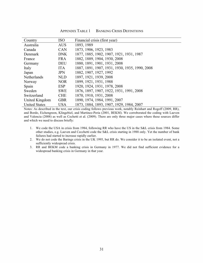
31

APPENDIX TABLE 1 BANKING CRISIS DEFINITIONS

Country ISO Financial crisis (first year) Australia AUS 1893, 1989 Canada CAN 1873, 1906, 1923, 1983 Denmark DNK 1877, 1885, 1902, 1907, 1921, 1931, 1987 France FRA 1882, 1889, 1904, 1930, 2008 Germany DEU 1880, 1891, 1901, 1931, 2008 Italy ITA 1887, 1891, 1907, 1931, 1930, 1935, 1990, 2008 Japan JPN 1882, 1907, 1927, 1992 Netherlands NLD 1897, 1921, 1939, 2008 Norway NOR 1899, 1921, 1931, 1988 Spain ESP 1920, 1924, 1931, 1978, 2008 Sweden SWE 1876, 1897, 1907, 1922, 1931, 1991, 2008 Switzerland CHE 1870, 1910, 1931, 2008 United Kingdom GBR 1890, 1974, 1984, 1991, 2007 United States USA 1873, 1884, 1893, 1907, 1929, 1984, 2007 Notes: As described in the text, our crisis coding follows previous work, notably Reinhart and Rogoff (2009, RR), and Bordo, Eichengreen, Klingebiel, and Martinez-Peria (2001, BEKM). We corroborated the coding with Laeven and Valencia (2008) as well as Cechetti et al. (2009). There are only three major cases where these sources differ and which we need to discuss briefly:

1. We code the USA in crisis from 1984, following RR who have the US in the S&L crisis from 1984. Some other studies, e.g. Laeven and Cecchetti code the S&L crisis starting in 1988 only. Yet the number of bank failures had started to increase rapidly earlier.

2. We do not code the Barings crisis in the UK 1995, but RR do. We consider it to be an isolated event, not a sufficiently widespread crisis.

3. RR and BEKM code a banking crisis in Germany in 1977. We did not find sufficient evidence for a widespread banking crisis in Germany in that year.

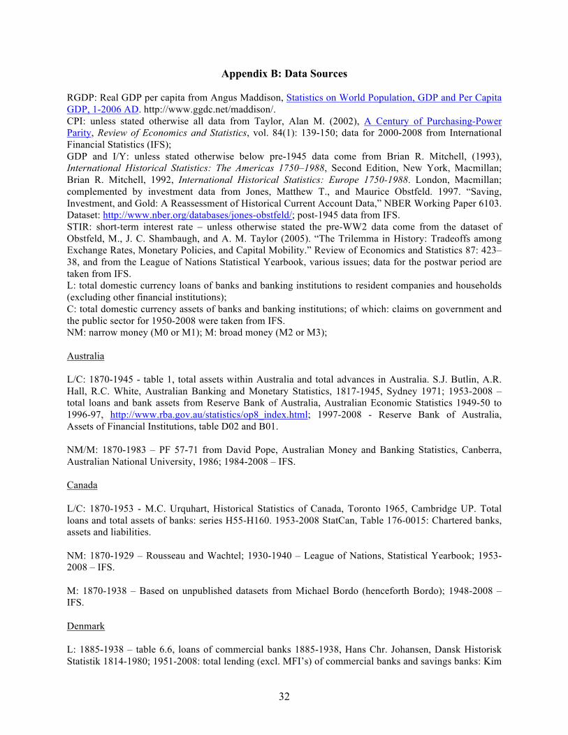
32

Appendix B: Data Sources RGDP: Real GDP per capita from Angus Maddison, Statistics on World Population, GDP and Per Capita GDP, 1-2006 AD. http://www.ggdc.net/maddison/. CPI: unless stated otherwise all data from Taylor, Alan M. (2002), A Century of Purchasing-Power Parity, Review of Economics and Statistics, vol. 84(1): 139-150; data for 2000-2008 from International Financial Statistics (IFS); GDP and I/Y: unless stated otherwise below pre-1945 data come from Brian R. Mitchell, (1993), International Historical Statistics: The Americas 1750–1988, Second Edition, New York, Macmillan; Brian R. Mitchell, 1992, International Historical Statistics: Europe 1750-1988. London, Macmillan; complemented by investment data from Jones, Matthew T., and Maurice Obstfeld. 1997. “Saving, Investment, and Gold: A Reassessment of Historical Current Account Data,” NBER Working Paper 6103. Dataset: http://www.nber.org/databases/jones-obstfeld/; post-1945 data from IFS. STIR: short-term interest rate – unless otherwise stated the pre-WW2 data come from the dataset of Obstfeld, M., J. C. Shambaugh, and A. M. Taylor (2005). “The Trilemma in History: Tradeoffs among Exchange Rates, Monetary Policies, and Capital Mobility.” Review of Economics and Statistics 87: 423–38, and from the League of Nations Statistical Yearbook, various issues; data for the postwar period are taken from IFS. L: total domestic currency loans of banks and banking institutions to resident companies and households (excluding other financial institutions); C: total domestic currency assets of banks and banking institutions; of which: claims on government and the public sector for 1950-2008 were taken from IFS. NM: narrow money (M0 or M1); M: broad money (M2 or M3); Australia L/C: 1870-1945 - table 1, total assets within Australia and total advances in Australia. S.J. Butlin, A.R. Hall, R.C. White, Australian Banking and Monetary Statistics, 1817-1945, Sydney 1971; 1953-2008 – total loans and bank assets from Reserve Bank of Australia, Australian Economic Statistics 1949-50 to 1996-97, http://www.rba.gov.au/statistics/op8_index.html; 1997-2008 - Reserve Bank of Australia, Assets of Financial Institutions, table D02 and B01. NM/M: 1870-1983 – PF 57-71 from David Pope, Australian Money and Banking Statistics, Canberra, Australian National University, 1986; 1984-2008 – IFS. Canada L/C: 1870-1953 - M.C. Urquhart, Historical Statistics of Canada, Toronto 1965, Cambridge UP. Total loans and total assets of banks: series H55-H160. 1953-2008 StatCan, Table 176-0015: Chartered banks, assets and liabilities. NM: 1870-1929 – Rousseau and Wachtel; 1930-1940 – League of Nations, Statistical Yearbook; 1953-2008 – IFS. M: 1870-1938 – Based on unpublished datasets from Michael Bordo (henceforth Bordo); 1948-2008 – IFS. Denmark L: 1885-1938 – table 6.6, loans of commercial banks 1885-1938, Hans Chr. Johansen, Dansk Historisk Statistik 1814-1980; 1951-2008: total lending (excl. MFI’s) of commercial banks and savings banks: Kim

33

Abildgren, Financial Liberalization and Credit Dynamics in Denmark in the Post-World War II Period, Danmarks Nationalbank, Working Papers 47/2007. C: table 6.6 - assets of commercial banks, Hans Chr. Johansen, Dansk Historisk Statistik; 1981-2008 – series L plus holdings of securities and other assets from OECD (2009). NM/M: 1870-1940 – table 6.2, 6.6, 6.8 in Hans Chr. Johansen, Dansk Historisk Statistik; 1950-2008 – IFS. France L: 1870-1940 from Saint Marc, Michelle, Histoire monétaire de la France, 1800-1980, Paris, 1983, who used credit data for Crédit lyonnais, Société général, Comptoir national d’escompte and Crédit industriel et commercial. She assumed that total loans in the French economy averaged about twice that amount before 1940; 1945 – 2008: data for 1945-1969 from Conseil National du Credit (data kindly shared by Eric Monnet, Paris); 1970-1984 from INSEE (“Crédit à l’économie de caractère bancaire”); 1985-2008 from Banque de France (MFI loans to private sector residents, A20.A.1.U6.2200.Z01). The pre-1895 loan data are subject to very crude rounding errors and are not used. NM: 1870-1940 from Saint Marc (1983); 1949-2008 from IFS (M1). M: 1920-1940 from Patat, Jean-Pierre and Michel Lutfalla, Histoire monétaire de la France au XXe siècle, Paris 1986; 1949-2008 from INSEE and Banque de France (M2). Germany L: 1880-1940 - table B1 1.05, total loans of Aktienbanken, Sparkassen, Hypothekenbanken and Genossenschaftsbanken; Deutsche Bundesbank, Deutsches Geld- und Bankwesen in Zahlen, 1876-1975, Fritz Knapp: Frankfurt am Main, 1976. 1948-2008 - Bundesbank, Lending to domestic non-banks (All categories of banks, OU01115). C: 1880-1940 - table A 1.01, total assets of Aktienbanken, Sparkassen, Hypothekenbanken and Genossenschaftsbanken; Deutsche Bundesbank, Deutsches Geld- und Bankwesen in Zahlen, 1876-1975, Fritz Knapp: Frankfurt am Main, 1976. 1950-2008 – Bundesbank: Balance sheet total (All categories of banks, OU0308). NM: 1876-1940 –Bundesbank (1976); 1950-2008 from IFS (M1). M: 1880-1940 from Bordo; 1950-2008 from IFS (M2). Japan L/C: 1870-1940 – Bank of Japan, Hundred-year statistics of the Japanese economy, Tokyo 1966 (Meiji-Iko Hompo Shuyo Keizaitokei); 1953-1982 – Tamaki, Norio, Japanese banking: a history, 1859 – 1959, Cambridge 1995, and IFS, 1983-2008 – Bank of Japan (series FA’FAABK_FAAB2DBEA40, Loans of domestically licensed banks less loans to other financial institutions); total domestic credit 1953-2008 from IFS. CPI: 1885-1940 – Obstfeld and Taylor (2003); 1950-2008 – IFS. NM: 1880-1940 – Bordo and Eichengreen (2001); 1955-2008 – IFS (M1).

34

M: 1901-1918 – Bordo; 1919-1940 – Mitchell; 1955-2008 – IFS (M2). STIR: 1870-1940 from Bank of Japan, Nihon Ginko Hyakunen-shi Shiryo-hen (Bank of Japan: The First Hundred Years-Materials), Tokyo 1986 - http://www.boj.or.jp/type/pub/hyakunen/hyakus.htm; 1950-2008 from IFS. Italy L/C: 1870-1940 – unpublished workfile: Gigliobianco, Alfredo and Claire Giordano and Gianni Toniolo, “Regulators and Innovators Play Tag: The Italian Historical Experience”, forthcoming. The data sources are De Mattia, R. (1967), I bilanci degli istitut idi emissione italiani 1845-1936, Vol. 1, Banca d’Italia: Rome, for the period 1870-1889;Cotula F. et al (1996), I bilanci delle aziende di credito 1890-1936, Editori Laterza: Rome- Bari, for the period 1890-1935; Unpublished data, Bank of Italy, for the period 1936-1973. 1950-1994 – Bank of Italy, total bank loans (S858159), extended 1995-2008 using growth rates from IFS and Bank of Italy (S515363M and S640592M, “lending to domestic non-financial enterprise and households”); assets 1950-2008 - Bank of Italy, series S049387, extended 1997-2008 using growth rates of banking sector assets from Bank of Italy (S463168M). NM/M: 1870-1939 M0 – Fratianni, M. and F. Spinelli, A Monetary History of Italy, Cambridge 1997; 1880-1945 M3 from Bordo; 1948-2008 - Bank of Italy, M1 and M2 Plus; after 1998 Italian contribution to Eurozone M1 and M3 from the Bank of Italy. Netherlands L: 1900-1982 sum of “Korte vorderingen op private sector”, “Onderhandse leningen”, “Hypothecaire leningen”, “Diverse binnenland active”, table 3.1 - De Nederlandsche Bank, Nederlandse financile instellingen in de twintigste eeuw: balansreeksen en naamlijst van handelsbanken, DNB Statistische Cahiers Nr.3, 2000; 1982-2008 DNB, Banking statistics, table 5.6ek. C: 1900-1945 Bilans total (excl. foreign assets) of commercial banks, table 3.1 - De Nederlandsche Bank, Nederlandse financile instellingen in de twintigste eeuw: balansreeksen en naamlijst van handelsbanken, DNB Statistische Cahiers Nr.3, 2000; 1948-2008 IFS (32) NM: 1900-1992 – Bordo and League of Nations; 1993-2008 – DNB, Table 5.4, Contribution of the Netherlands to euro area monetary aggregates, Guilder M1; 1945-1998 – IFS; 1999-2008 – DNB, Table 5.4, Contribution of the Netherlands to euro area monetary aggregates, Guilder M3. GDP and I/Y: 1880-1913 – van Zanden et al., National Accounts of the Netherlands 1880-1913; http://nationalaccounts.niwi.knaw.nl/start.htm; 1918-1940 – Mitchell; 1948-2008 – IFS. Norway L/C: table A2 and A4, Eitrheim/Klovland/Qvigstad (eds), Historical Monetary Statistics for Norway, Chapter 10: Credit, banking and monetary developments in Norway, Norges Banks Occasional Papers nr. 35, Oslo 2004.Datafile: http://www.norges-bank.no/templates/article____42927.aspx NM/M: table 2a, monetary aggregates in Norway,Norges Bank: http://www.norges-bank.no/templates/article____42935.aspx

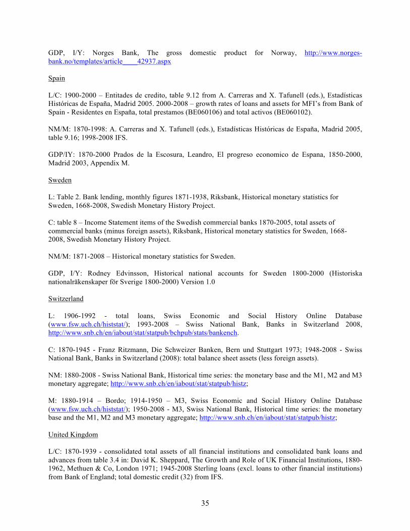
35

GDP, I/Y: Norges Bank, The gross domestic product for Norway, http://www.norges-bank.no/templates/article____42937.aspx Spain L/C: 1900-2000 – Entitades de credito, table 9.12 from A. Carreras and X. Tafunell (eds.), Estadísticas Históricas de España, Madrid 2005. 2000-2008 – growth rates of loans and assets for MFI’s from Bank of Spain - Residentes en España, total prestamos (BE060106) and total activos (BE060102). NM/M: 1870-1998: A. Carreras and X. Tafunell (eds.), Estadísticas Históricas de España, Madrid 2005, table 9.16; 1998-2008 IFS. GDP/IY: 1870-2000 Prados de la Escosura, Leandro, El progreso economico de Espana, 1850-2000, Madrid 2003, Appendix M. Sweden L: Table 2. Bank lending, monthly figures 1871-1938, Riksbank, Historical monetary statistics for Sweden, 1668-2008, Swedish Monetary History Project. C: table 8 – Income Statement items of the Swedish commercial banks 1870-2005, total assets of commercial banks (minus foreign assets), Riksbank, Historical monetary statistics for Sweden, 1668-2008, Swedish Monetary History Project. NM/M: 1871-2008 – Historical monetary statistics for Sweden. GDP, I/Y: Rodney Edvinsson, Historical national accounts for Sweden 1800-2000 (Historiska nationalräkenskaper för Sverige 1800-2000) Version 1.0 Switzerland L: 1906-1992 - total loans, Swiss Economic and Social History Online Database (www.fsw.uch.ch/histstat/); 1993-2008 – Swiss National Bank, Banks in Switzerland 2008, http://www.snb.ch/en/iabout/stat/statpub/bchpub/stats/bankench. C: 1870-1945 - Franz Ritzmann, Die Schweizer Banken, Bern und Stuttgart 1973; 1948-2008 - Swiss National Bank, Banks in Switzerland (2008): total balance sheet assets (less foreign assets). NM: 1880-2008 - Swiss National Bank, Historical time series: the monetary base and the M1, M2 and M3 monetary aggregate; http://www.snb.ch/en/iabout/stat/statpub/histz; M: 1880-1914 – Bordo; 1914-1950 – M3, Swiss Economic and Social History Online Database (www.fsw.uch.ch/histstat/); 1950-2008 - M3, Swiss National Bank, Historical time series: the monetary base and the M1, M2 and M3 monetary aggregate; http://www.snb.ch/en/iabout/stat/statpub/histz; United Kingdom L/C: 1870-1939 - consolidated total assets of all financial institutions and consolidated bank loans and advances from table 3.4 in: David K. Sheppard, The Growth and Role of UK Financial Institutions, 1880-1962, Methuen & Co, London 1971; 1945-2008 Sterling loans (excl. loans to other financial institutions) from Bank of England; total domestic credit (32) from IFS.

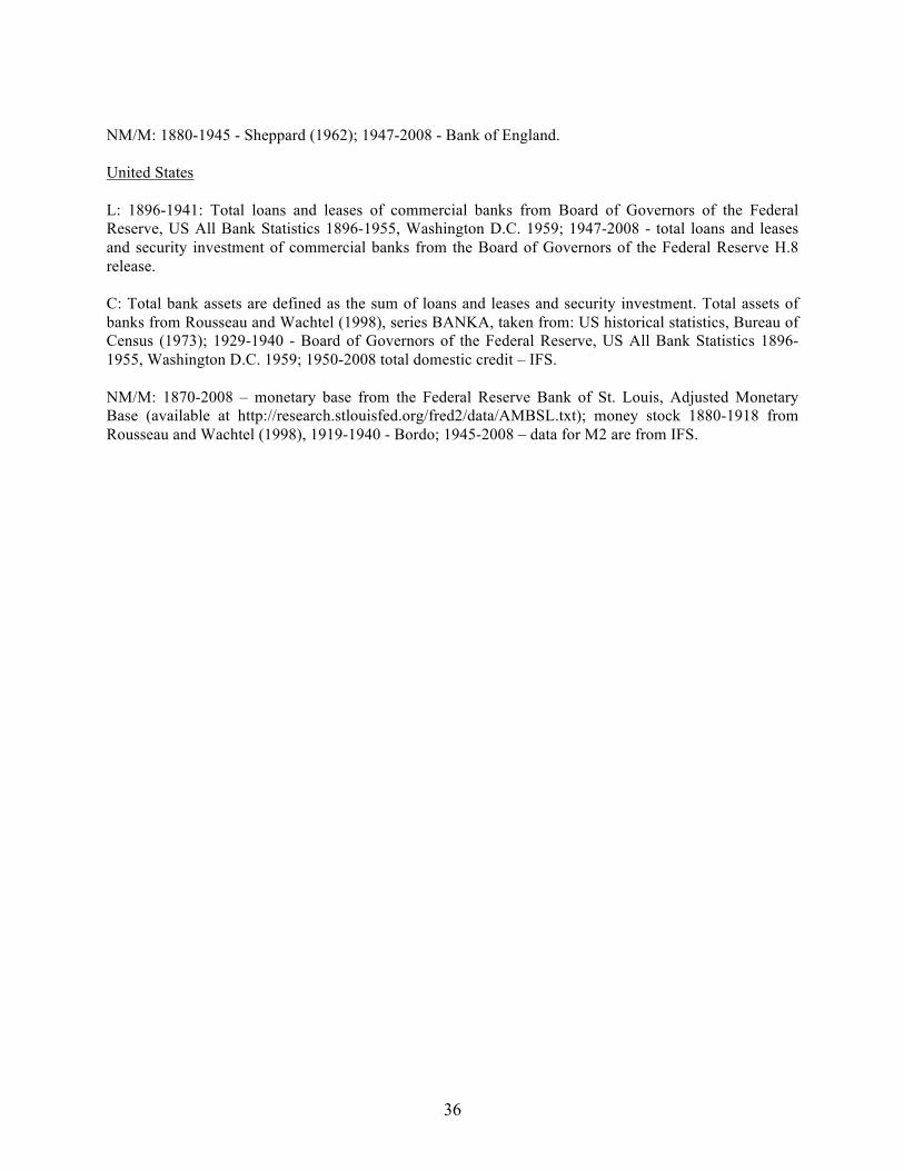
36

NM/M: 1880-1945 - Sheppard (1962); 1947-2008 - Bank of England. United States L: 1896-1941: Total loans and leases of commercial banks from Board of Governors of the Federal Reserve, US All Bank Statistics 1896-1955, Washington D.C. 1959; 1947-2008 - total loans and leases and security investment of commercial banks from the Board of Governors of the Federal Reserve H.8 release. C: Total bank assets are defined as the sum of loans and leases and security investment. Total assets of banks from Rousseau and Wachtel (1998), series BANKA, taken from: US historical statistics, Bureau of Census (1973); 1929-1940 - Board of Governors of the Federal Reserve, US All Bank Statistics 1896-1955, Washington D.C. 1959; 1950-2008 total domestic credit – IFS. NM/M: 1870-2008 – monetary base from the Federal Reserve Bank of St. Louis, Adjusted Monetary Base (available at http://research.stlouisfed.org/fred2/data/AMBSL.txt); money stock 1880-1918 from Rousseau and Wachtel (1998), 1919-1940 - Bordo; 1945-2008 – data for M2 are from IFS.

37

References Almunia, Miguel, Agustín S. Bénétrix, Barry Eichengreen, Kevin H. O’Rourke, and Gisela Rua. 2009.

From Great Depression to Great Credit Crisis: Similarities, Differences and Lessons. Economic Policy. Forthcoming.

Arellano, Manuel, and Olympia Bover. 1995. Another Look at the Instrumental Variable Estimation in Error-Component Models. Journal of Econometrics 68: 28–51.

Adrian, Tobias, and Hyun Song Shin. 2008. Liquidity and Financial Cycles. BIS Working Papers No. 256, July 2008.

Adrian, Tobias, and Hyun Song Shin. 2009. Money, Liquidity, and Monetary Policy. FRBNY Staff Report 360, January.

Barro, Robert J. 2009. Rare Disasters, Asset Prices, and Welfare Costs. American Economic Review 99(1): 243–64.

Bernanke, Ben S, 1983. Nonmonetary Effects of the Financial Crisis in Propagation of the Great Depression. American Economic Review 73(3): 257–76.

Bernanke, Ben S. 1993. Credit in the Macroeconomy. Quarterly Review, Federal Reserve Bank of New York, Spring, pp. 50–70.

Bernanke, Ben S., and Alan S. Blinder. 1992. The Federal Funds Rate and the Channels of Monetary Transmission. American Economic Review 82(4): 901–21.

Bernanke, Ben S., and Mark Gertler. 1995. Inside the Black Box: The Credit Channel of Monetary Policy Transmission. Journal of Economic Perspectives 9(4): 27–48.

Bernanke, Ben S., Mark Gertler, and Simon Gilchrist. 1999. The financial accelerator in a quantitative business cycle framework. In Handbook of Macroeconomics, vol. 1, edited by J. B. Taylor and M. Woodford. Amsterdam: Elsevier, pp. 1341–93.

Biggs, Michael, Thomas Mayer, and Andreas Pick. 2009. Credit and economic recovery. DNB Working Papers 218, Netherlands Central Bank, Research Department.

Bordo, Michael, Barry Eichengreen, Daniela Klingebiel, and Maria Soledad Martinez-Peria. 2001. Is the crisis problem growing more severe? Economic Policy 16(32): 51–82.

Borio, Claudio. 2008. The financial turmoil of 2007–?: a preliminary assessment and some policy considerations. BIS Working Papers no. 251.

Borio, Claudio, Craig Furfine, and Philip Lowe. 2001. Procyclicality of the financial system and financial stability: issues and policy options. BIS Papers, no. 1.

Borio, Claudio, and Philip Lowe. 2002. Asset Prices, Financial and Monetary Stability: Exploring the Nexus. BIS Working Papers 114, Bank for International Settlements.

Borio, Claudio, and Philip Lowe. 2003. Imbalance or “Bubbles?” Implications for Monetary and financial Stability. In Asset Price Bubbles: The Implications for Monetary, Regulatory, and International Policies, edited by W. C. Hunter, G. C. Kaufman, and M. Pomerleano. Cambridge, Mass.: MIT Press, pp. 247–70.

Borio, Claudio, and William R. White. 2003. Whither Monetary and Financial Stability: The Implications of Evolving Policy Regimes. Proceedings, Federal Reserve Bank of Kansas City, pp. 131–211.

Cecchetti, Stephen G., Marion Kohler, and Christian Upper. 2009. Financial Crises and Economic Activity. NBER Working Papers 15379.

Chari, V. V., Lawrence J. Christiano, and Patrick J. Kehoe. 2008. Facts and Myths About the Financial Crisis of 2008.Working Paper no. 666, Federal Reserve Bank of Minneapolis.

Chernyshoff, Natalia, David S. Jacks, and Alan M. Taylor. 2009. “Stuck on Gold: Real Exchange Rate Volatility and the Rise and Fall of the Gold Standard, 1875–1939. Journal of International Economics 77(April): 195–205.

Christiano, Lawrence, Roberto Motto, and Massimo Rostagno. 2007. Two Reasons Why Money and Credit May be Useful in Monetary Policy. NBER Working Paper No. 13502.

Demirgüç-Kunt, Asli, and Enrica Detragiache. 1998. The Determinants of Banking Crises in Developing and Developed Countries. IMF Staff Papers 45(1): 81–109.

38

Eckstein, Otto, and Allen Sinai. 1986. The mechanisms of the business cycle in the postwar era. In The American Business Cycle in the Postwar Era: Continuity and Change, edited by Robert J. Gordon. Chicago: University of Chicago Press.

Edwards, Sebastian. 2002. Does the Current Account Matter? In Preventing Currency Crises in Emerging Markets, edited by Sebastian Edwards and Jeffrey Frankel. Chicago: University of Chicago Press, pp. 21–75.

Eichengreen, Barry. 2009. The Last Temptation of Risk. The National Interest (May/ June): 8–14. Eichengreen, Barry, and Mitchener, Kris J. 2003. The Great Depression as a Credit Boom Gone Wrong.

BIS Working Paper No. 137, September. Eichengreen, Barry, and Carlos Arteta. 2002. Banking Crises in Emerging Markets: Presumptions and

Evidence. In Financial Policies in Emerging Markets edited by Mario Blejer and Marko Škreb. Cambridge, Mass.: MIT Press, pp. 47–94.

Farhi, Emmanuel, and Jean Tirole. 2009. Collective Moral Hazard, Maturity Mismatch and Systemic Bailouts. NBER Working Papers 15138.

Fisher, Irving. 1933. The Debt-Deflation Theory of Great Depressions. Econometrica 1(4): 337–57. Freixas, Xavier, and Jean-Charles Rochet. 1997. Microeconomics of Banking. Cambridge, Mass.: MIT

Press. Friedman, Benjamin M., and Kenneth N. Kuttner. 1992. Money, Income, Prices, and Interest Rates.

American Economic Review 82: 472–92. Friedman, Milton, and Anna J. Schwartz. 1963. A Monetary History of the United States: 1867–1960.

Princeton, N. J.: Princeton University Press. Geanakoplos, John. 2009. The Leverage Cycle. Cowles Foundation Discussion Papers 1715, Cowles

Foundation, Yale University. Gertler, Mark. 1988. Financial Structure and Aggregate Economic Activity: An Overview. Journal of

Money, Credit and Banking 20(3): 559–88. Goldsmith, Raymond W. 1969. Financial Structure and Development. New Haven, Conn.: Yale

University Press. Goodhart, Charles. 2007. Whatever Became of the Monetary Aggregates? Peston Lecture, delivered at

Queen Mary College, London, on February 28, 2007 Goodhart, Charles A. E., and Boris Hofmann. 2008. House prices, money, credit and the. macroeconomy.

Working Paper Series 888, European Central Bank. Gourinchas, Pierre-Olivier, Rodrigo O. Valdes, and Oscar Landerretche. 2001.Lending Booms: Latin

America and the World. Economía 1 (2): 47–99. Gurley, John G., and E. S. Shaw. 1955. Financial Aspects of Economic Development. American

Economic Review 45(September): 515–38. Hume, Michael, and Andrew Sentance. 2009. The Global Credit Boom: Challenges for Macroeconomics

and Policy. External MPC Unit Discussion Paper No. 27, Bank of England, June. Jermann, Urban, and Vincenzo Quadrini, 2009.Macroeconomic Effects of Financial Shocks. NBER

Working Papers 15338, September. Jung, Woo S. 1986. Financial Development and Economic Growth: International Evidence. Economic

Development and Cultural Change 34(2): 333–46. Kaminsky, Graciela L., and Carmen M. Reinhart. 1999. The Twin Crises: The Causes of Banking and

Balance-of-Payments Problems. American Economic Review 89(3): 473–500. Kashyap, Anil K., Raghuram G. Rajan, and Jeremy C. Stein. 2008. Rethinking Capital Regulation.

Proceedings, Federal Reserve Bank of Kansas City, pp. 431–471. Kaufman, Henry. 1986. Debt: the threat to economic and financial stability. Economic Review, Federal

Reserve Bank of Kansas City, December, pp. 3–11. Kindleberger, Charles P. 1978. Manias, Panics, and Crashes: A History of Financial Crises. New York:

Basic Books. King, Robert G., and Ross Levine. 1993. Finance and Growth: Schumpeter Might Be Right. Quarterly

Journal of Economics 108: 717–27.

39

Kiyotaki, Nobuhiro, and John Moore. 1997. Credit Cycles. Journal of Political Economy 105(2): 211–48. Laeven, Luc, and Fabian Valencia. 2008. Systemic Banking Crises: A New Database. IMF Working

Paper 08/224, November. McKinnon, Ronald I. 1973. Money and Capital in Economic Development. Washington, D.C.: Brookings

Institution. McKinnon, Ronald I.,and HuwPill. 1997. Credible Economic Liberalizations and Overborrowing.

American Economic Review 87(2): 189–93. Mendoza, Enrique G., and Marco E. Terrones, 2008. An Anatomy Of Credit Booms: Evidence From

Macro Aggregates And Micro Data. NBER Working Papers 14049. Minsky, Hyman P. 1977. The Financial Instability Hypothesis: an Interpretation of Keynes and

Alternative to Standard Theory. Challenge (March–April): 20–27. Mishkin, Frederic S., 1978. The Household Balance Sheet and the Great Depression. Journal of

Economic History 38: 918–37. Modigliani, Franco, and Merton Miller. 1958. The Cost of Capital, Corporation Finance and the Theory

of Investment. American Economic Review 48(3): 261–97. Nolan, Charles, and Christoph Thoenissen. 2009.Financial Shocks and the U.S. Business Cycle. Journal

of Monetary Economics 56(4): 596–604. Pepe, Margaret S. 2003. The Statistical Evaluation of Medical Tests for Classification and Prediction.

Oxford: Oxford University Press. Rajan, Raghuram G. 2005. Has financial development made the world riskier? Proceedings, Federal

Reserve Bank of Kansas City, pp. 313–369. Reinhart, Carmen M., and Kenneth S. Rogoff. 2009. This Time is Different: Eight Centuries of Financial

Folly. Princeton, N.J.: Princeton University Press. Rousseau, Peter L., and Paul Wachtel. 1998. Financial Intermediation and Economic Performance:

Historical Evidence from Five Industrialized Countries. Journal of Money, Credit and Banking 30(4): 657–78.

Shaw, E. S. 1973. Financial Deepening in Economic Development. Oxford: Oxford University Press. Turner, Adair. 2009. The Turner Review: A Regulatory Response to the Global Banking Crisis. London:

Financial Services Authority. Woodford, Michael. 2003. Interest and Prices: Foundations of a Theory of Monetary Policy. Princeton,

N.J.: Princeton University Press. White, William R. 2006. Is Price Stability Enough? BIS Working Papers, no. 205, April.