Credit: 2 PDH

Course Title: Mechanical Characterization of Laminated Rubber

Bearings and Their Modeling Approach

3 Easy Steps to Complete the Course:

1. Read the Course PDF

2. Purchase the Course Online & Take the Final Exam

3. Print Your Certificate

Approved for:AK, AL, AR, DE, GA, IA, ID, IL, KS, KY, LA, ME, MI, MN, MO, MS, MT, ND, NE, NH, NM, NV, OK, OR, PA, SC, SD, TN, TX, UT, VT, VA, WI, WV, WY

epdh.com is a division of Cer�fied Training Ins�tute

Mechanical Characterization of Laminated

Rubber Bearings and Their Modeling

Approach

A. R. Bhuiyan1 and Y. Okui2

[1] Department of Civil Engineering, Chittagong University of Engineering and Technology,

Chittagong, Bangladesh

[2] Department of Civil and Environmental Engineering, Saitama University, Saitama, Japan

1. Introduction

Base isolation, also known as seismic base isolation, is one of the most popular means of

protecting a structure against earthquake forces. It is a collection of structural elements which

should substantially decouple a superstructure from its substructure resting on a shaking ground

thus protecting building and bridge structure's integrity.Base isolation is the most powerful tool

of earthquake engineering pertaining to the passive structural vibration control technologies. It is

meant to enable building and bridge structure to survive a potentially devastating seismic impact

through a proper initial design or subsequent modifications. In some cases, application of base

isolation can raise both a structure's seismic performance and its seismic sustainability

considerably.

An isolation system is believed to be able to support a structure while providing additional

horizontal flexibility and energy dissipation. Until the 80th decade of the last century many

systems have been put forward involving features such as rollers or rockers bearings, sliding on

sand or talc, or complaint first story column, but these have usually not employed in the practice

of isolation of engineering structures [1, 2]. The study on the mechanical behavior of the

isolation system dates back to 1886, when Professor Milne from Tokyo University, Japan

attempted to observe isolation behavior of a structure supported by balls.He conducted an

experiment by making an isolated building supported on balls “cast-iron plates with saucer-like

edges on heads of piles. Above the balls and attached to the buildings are cast-iron plates

slightly concave but otherwise similar to those below” [3]. However, another guy J.A.

Calantarients in 1909, a medical doctor of the northern EnglishCity of Scarborough, was claimed

to be the first man who conducted the experiment of isolation behavior of a structure supported

by balls [3]. What both guys wanted to get information from their experiments is the global

isolation behavior of the structure. The philosophy given by them regarding seismic isolation of

a structure is stillin practice. Several mechanisms of investigating the mechanical behavior of

isolation systems are developed based on this philosophy which is readily used.

In practice of seismic base isolation of bridge structures, laminated rubber bearings have been

popular since the last century. Among many types of laminated rubber bearings, natural rubber

bearing (RB) which is formed by alternate layers of unfilled rubbers and steel shims has less

flexibility and small damping. It has been used to sustain the thermal movement, the effect of

pre-stressing, creep and shrinkage of the superstructures of the bridge or has been used for base

isolation practices with additional damping devices [1, 2 and 4]. On the other hand, other two

types of bearings possessing high damping were developed and have widely used in the seismic

isolation practices [1, 3]. One is the lead rubber bearing (LRB), which additionally inserts lead

plugs down the center of RB to enhance the hysteretic damping, and the other is high damping

rubber bearing (HDRB), whose rubber material possesses high damping in order to supply more

dissipating energy.

Following the same principle as Professor Milne used in his experiments, several authors

conducted experimental studies on different bridge structures mounted on laminated rubber

bearings. Kelly et al. [5] studied quarter-scale models of straight and skewed bridge decks

mounted on plain and lead-filled elastomeric bearings subjected to earthquake ground motion

using the shaking table. The deck response was compared to determine the effectiveness of

mechanical energy dissipaters in base isolation systems and the mode of failure of base-isolated

bridges. Igarashi and Iemura [6] evaluated the effects of implementing the lead-rubber bearing as

seismic isolator on a highway bridge structure under seismic loads using the substructure hybrid

loading (pseudo-dynamic) test method. The seismic response of the isolated bridge structure was

successfully obtained. The effectiveness of isolation is examined based on acceleration and

displacement amplifications using earthquake response results.All of their studies were related to

observation of the isolation effects on the bridge structures.Very few works were undertaken in

the past regarding the mechanical behavior of isolation bearings.

Mori et al. [7, 8] studied the behavior of laminated bearings with and without lead plug under

shear and axial loads. They evaluated hysteretic parameters of the bearings: horizontal stiffness;

vertical stiffness; and equivalent damping ratio. The similar study was conducted by Burstscher

et al. [9]; Fujita et al. [10]; Mazda et al. [11] and Ohtori et al. [12] on lead, natural and high

damping rubber bearings. They concluded from the experimental results that the hysteretic

parameters have low loading rate-dependence. Furthermore, Robinson[13], a pioneer of

developing and introducing the lead rubber bearing (LRB) as an excellent isolation system to be

used in seismic design of civil engineering structures, conducted an elaborate experimental tests

on LRB in order to describe the hysteretic behavior. From the experiments he concluded that the

hysteretic behavior of the LRB can be expressed well by using a bilinear relationship of the

force-displacements. In addition, he conducted some tests regarding fatigue and temperature

performance of the LRB.

Several authors conducted different loading experiments on laminated rubber bearings (RB,

LRB, and HDRB) in order to acquire deep understanding of the mechanical properties. In this

case the works of Abe et al. [14]; Aiken et al. [15]; Kikuchi and Aiken [16]; Sano and D

Pasquale [17] can be noted. They have applied uni-directional and bi-directional horizontal shear

deformations with constant vertical compressive stress. Several types of laminated rubber

bearings were used in their experimental scheme. In their investigationsthey identified some

aspects of the bearings such as hardening features and dependence of the restoring forces on the

maximum displacement amplitude experienced in the past. Moreover, some of them also

identified coupling effects on the restoring forces of the bearings due to deformation in the two

horizontal directions. Motivated by the experimental results of the bearings different forms of

analytical models of the bearings were proposed by them. However, their studies were mostly

related to illustrating the strain-rate independent mechanical behavior of the bearings.

Very few works are reported in literature regarding the strain-rate dependent behavior of the

bearings. In this regard, the works of Dall’Asta and Ragni[18]; Hwang et al. [19] and Tsai et al.

[20] can be reported. They studied the mechanical behavior of high damping rubber dissipating

devices by conducting different experiments such as sinusoidal loading tests at different

frequencies, simple cyclic shear tests at different strain-rates along with relaxation tests. From

the experiments they have identified the strain-rate dependence of the restoring forces and

subsequently developed rate-dependent analytical models of the bearings. Strain-rate dependent

Mullin’s softening was also identified in the experiments [18]. However, separation of the rate-

dependent behavior from other mechanical behavior of the bearings was not elaborately

addressed in their studies.

A number of experimental and numerical works on different rubber materials (HDR: high

damping rubber and NR: natural rubber) have been performed in the past [21-27]. These works

show that the mechanical properties of rubber materials (especially HDR) are dominated by the

nonlinear rate-dependence including other inelastic behavior. Moreover, the different viscosity

behavior in loading and unloading has been identified [21, 23, 28 and 29].

It is well known that since seismic response of base isolated structures greatly depends on

mechanical properties of the bearings, deep understanding of the characteristics of the bearings

under the desired conditions is very essential for rational and economic design of the seismic

isolation system. The general mechanical behavior of laminated rubber bearings mainly concerns

with nonlinear rate-dependent hysteretic property [18, 19] in addition to other inelastic behavior

like Mullin’s softening effect [30] and relaxation behavior [31]. All these characteristic

behaviors generally originate from the molecular structures of the strength elements of rubber

materials used in manufacturing of the bearings.Within this context, the chapter is devoted to

discuss an experimental scheme used to characterize mechanical behavior and subsequently

develop a mathematical model representing the characteristicbehavior of the bearings.

2. Experimental observation

The objective of the work is to make qualitative and quantitative studies of strain-rate

dependency of the bearings subjected to horizontal shear deformation with a constant vertical

compressive load. To this end, an experimental scheme comprisedof multi-step relaxation tests,

cyclic shear tests, and simple relaxation tests was conducted: the mutli-step relaxation tests were

carried out to investigate the strain-rate independent behavior along with viscosity behavior in

loading and unloading; the cyclic shear tests, to observe the strain-rate dependency; and the

simple relaxation tests, to describe the viscosity behavior of the bearings. To separate the

Mullins’ effect from other inelastic effects, a preloading sequence was applied on each specimen

prior to the actual test. Details of the experiments and the inferences observed therein are

described in the following subsections.

2.1. Specimens

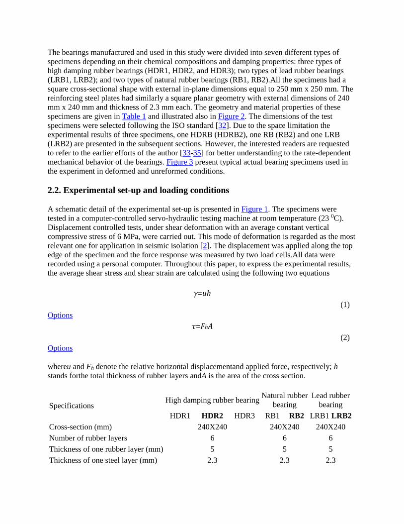
The bearings manufactured and used in this study were divided into seven different types of

specimens depending on their chemical compositions and damping properties: three types of

high damping rubber bearings (HDR1, HDR2, and HDR3); two types of lead rubber bearings

(LRB1, LRB2); and two types of natural rubber bearings (RB1, RB2).All the specimens had a

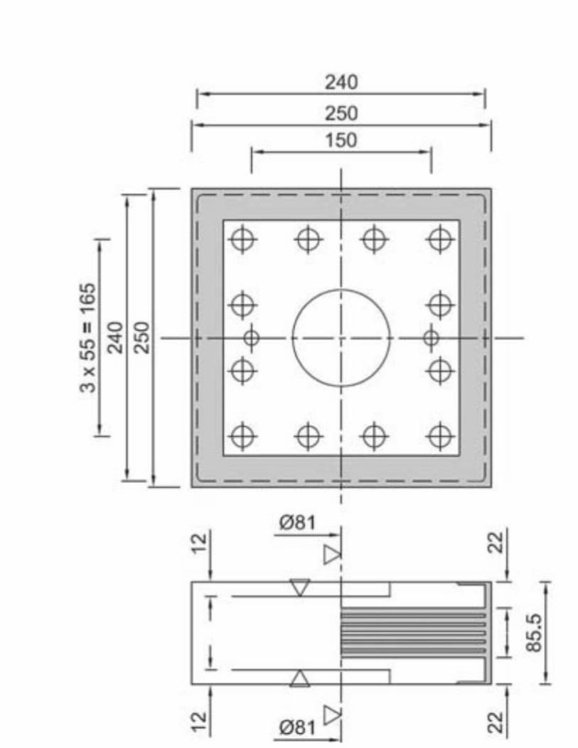
square cross-sectional shape with external in-plane dimensions equal to 250 mm x 250 mm. The

reinforcing steel plates had similarly a square planar geometry with external dimensions of 240

mm x 240 mm and thickness of 2.3 mm each. The geometry and material properties of these

specimens are given in Table 1 and illustrated also in Figure 2. The dimensions of the test

specimens were selected following the ISO standard [32]. Due to the space limitation the

experimental results of three specimens, one HDRB (HDRB2), one RB (RB2) and one LRB

(LRB2) are presented in the subsequent sections. However, the interested readers are requested

to refer to the earlier efforts of the author [33-35] for better understanding to the rate-dependent

mechanical behavior of the bearings. Figure 3 present typical actual bearing specimens used in

the experiment in deformed and unreformed conditions.

2.2. Experimental set-up and loading conditions

A schematic detail of the experimental set-up is presented in Figure 1. The specimens were

tested in a computer-controlled servo-hydraulic testing machine at room temperature (23 0C).

Displacement controlled tests, under shear deformation with an average constant vertical

compressive stress of 6 MPa, were carried out. This mode of deformation is regarded as the most

relevant one for application in seismic isolation [2]. The displacement was applied along the top

edge of the specimen and the force response was measured by two load cells.All data were

recorded using a personal computer. Throughout this paper, to express the experimental results,

the average shear stress and shear strain are calculated using the following two equations

γ=uh (1)

Options

τ=FhA (2)

Options

whereu and Fh denote the relative horizontal displacementand applied force, respectively; h

stands forthe total thickness of rubber layers andA is the area of the cross section.

Specifications High damping rubber bearing

Natural rubber

bearing

Lead rubber

bearing

HDR1 HDR2 HDR3 RB1 RB2 LRB1 LRB2

Cross-section (mm) 240X240 240X240 240X240

Number of rubber layers 6 6 6

Thickness of one rubber layer (mm) 5 5 5

Thickness of one steel layer (mm) 2.3 2.3 2.3

Diameter of lead plug (mm) - - 34.5

No of lead plugs - - 4

Nominal shear modulus (MPa) 1.2 1.2 1.2

Table 1.

Geometry and material properties of the bearings

2.2.1. Softening behavior

Virgin rubber typically exhibits a softening phenomenon, known as Mullins’ effect in its first

loading cycle. Due to presence of this typical behavior, the first cycle of a stress-strain curve

differs significantly from the shape of the subsequent cycles [30]. In order to remove the Mullins

softening behavior from other inelastic phenomena, all specimens were preloaded before the

actual tests. The preloading was done by treating 11 cycles ofsinusoidal loading at 1.75 strain

and 0.05 Hz until a stable state of the stress-strain response is achieved, i.e., that no further

softening occurs. The strain histories as applied in preloading sequence are shown in Figure 4.

Figures 5 (a), (b), and (c) present the typical shear stress-strain responses obtained from pre-

loading tests on HDR2,RB2 and LRB2 specimens.The same loading sequence was applied on

two types of specimens: virgin specimens and preloading specimens. The virgin specimen was

loaded first with the prescribed loading sequence and then the same specimen (known as the

preloading specimen) was again loaded with same loading sequence. The time interval between

these two loading sequences was 30 min. The softening behavior in the first loading cycle is

evident from Figure 5 in each specimen (virgin and preloading) indicating that the Mullins

softening effect is not only present in the virgin specimen but also in any preloaded specimen

[18]. This implies that Mullins effect can be recovered in quite a very short period. This is

certainly due to the ‘healing effect’ [36, 37]. As can be seen from Figures 5 (a) to (c), the

softening behavior is more appreciably well-defined in HDR2 than LRB2 and RB2. All the

specimens have shown a repeatable stress-stretch response after passing through 4-5 loading

cycles indicating that the Mullin’s softening effect of the bearings is removed from the other

effects.

2.2.2. Strain-rate dependent behavior

With a view to understanding the mechanical behavior of the bearings regarding the strain rate-

dependence, cyclic shear tests (CS tests) at different strain rates were carried out. In the test

series, a number of constant strain-rate cases within a range of 0.05/s to 5.5/s were considered as

shown in Figure 6. Figures 7 (a), (b), and (c) show the strain-rate dependent shear stress

responses of HDR2, RB2, and LRB2 bearings, respectively. For comparison, the equivalent

stress responses of the bearings are also represented in each Figure. The equivalent stress

responses of the bearings can be identified from MSR test results (Section 2.2.4).

https://www.intechopen.com/source/html/38206/media/image3.jpeg

Figure 1.

Schematic details of the experimental set-up. All dimensions are in mm

In general, the stress responses in the loading path contain three-characteristic features like a

high initial stiffness feature at low strain levels followed by a traceable large flexibility at

moderate strain levels as well as a large strain-hardening feature at the end. The untangling

and/or the separation of weak bonds between filler particles and long chains are associated with

reduced effect of the high initial stiffness [38]. This typical phenomenon is regarded the ‘Payne

effect’ [25]. The final increase of the stiffness is attributed to the limited extensibility of the

polymer chains and may be endowed to the ‘strain hardening’ feature [38]. When compared

among the three bearings, the high initial stiffness at a low strain level and the high strain

hardening at a high strain level are mostly prominent in HDR2 at a higher strain rates. However,

a weaker strain-hardening feature in LRB2 than the other specimen (RB2) at higher strain levels

is also noticeable.A comparison of hysteresis loops observed at different strain rates shows that

the size of the hysteresis loops increases with increase of strain rates as shown in Figures7 (a) to

(c). While comparing among all the bearings, HDR2 demonstrates a bigger hysteresis loop

compared with the other bearings (RB2 and LRB2). This typical behavior can be attributed that

the HDR2 inherits relatively high viscosity property than in other bearings. The addition of

special chemical compounds in manufacturing process enhances the damping property of the

HDRB.

https://www.intechopen.com/source/html/38206/media/image4.jpeg

Figure 2.

Dimension of a specimens [mm] (a) plan view (b) sectional view

Figure 3.

Typical bearing specimens used in the experiment in (a) un-deformed and (b) deformed

condition

Figure 4.

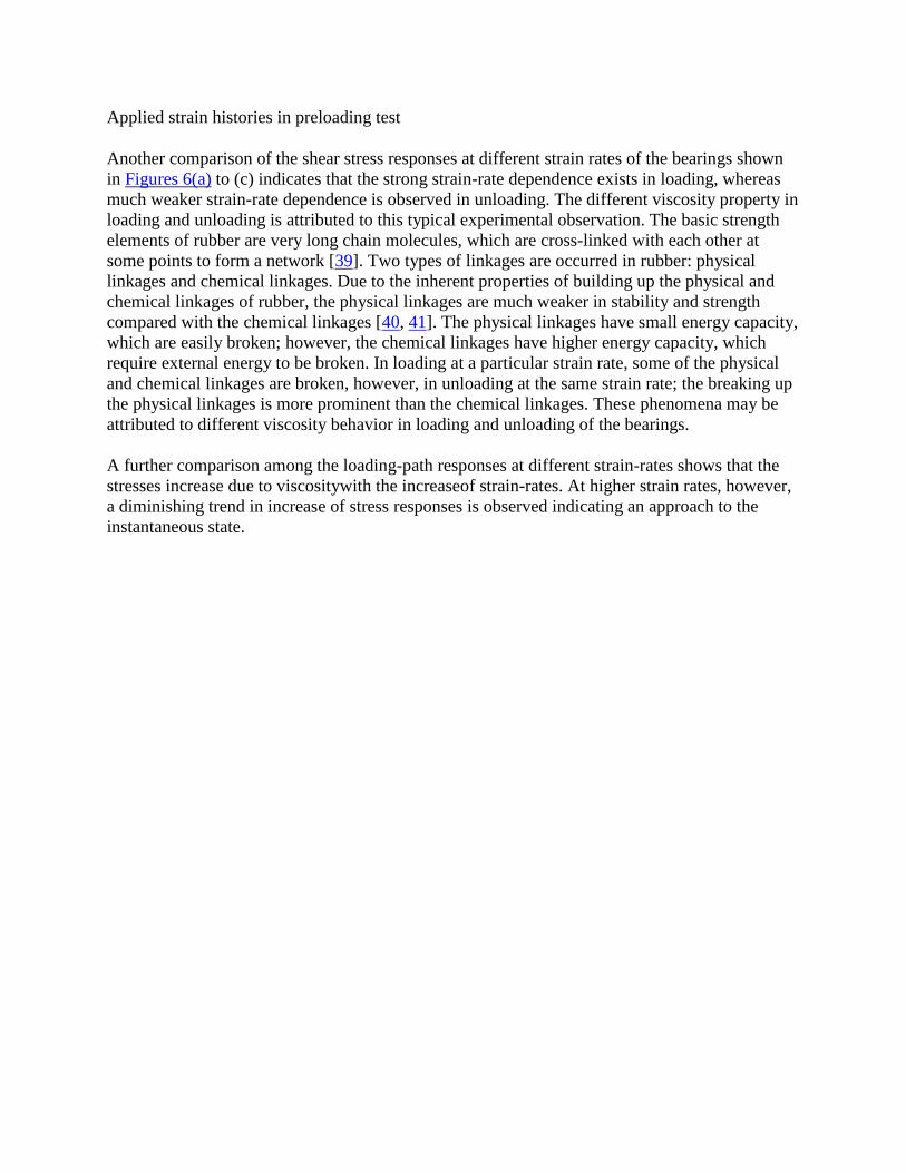
Applied strain histories in preloading test

Another comparison of the shear stress responses at different strain rates of the bearings shown

in Figures 6(a) to (c) indicates that the strong strain-rate dependence exists in loading, whereas

much weaker strain-rate dependence is observed in unloading. The different viscosity property in

loading and unloading is attributed to this typical experimental observation. The basic strength

elements of rubber are very long chain molecules, which are cross-linked with each other at

some points to form a network [39]. Two types of linkages are occurred in rubber: physical

linkages and chemical linkages. Due to the inherent properties of building up the physical and

chemical linkages of rubber, the physical linkages are much weaker in stability and strength

compared with the chemical linkages [40, 41]. The physical linkages have small energy capacity,

which are easily broken; however, the chemical linkages have higher energy capacity, which

require external energy to be broken. In loading at a particular strain rate, some of the physical

and chemical linkages are broken, however, in unloading at the same strain rate; the breaking up

the physical linkages is more prominent than the chemical linkages. These phenomena may be

attributed to different viscosity behavior in loading and unloading of the bearings.

A further comparison among the loading-path responses at different strain-rates shows that the

stresses increase due to viscositywith the increaseof strain-rates. At higher strain rates, however,

a diminishing trend in increase of stress responses is observed indicating an approach to the

instantaneous state.

https://www.intechopen.com/source/html/38206/media/image7.jpeg

Figure 5.

cycle preloading test on the bearings to remove Mullins effect; (a) HDR2, (b) RB2, (c) LRB2;

the legend indicates that the solid line in each Figure shows the shear stress histories obtained

from the virgin specimens and the dotted line does for the preloading specimens. For clear

illustration the shear stress-strain responses are separated by 0.15 sec from each other

Figure 6.

Applied strain histories in CS tests.

https://www.intechopen.com/source/html/38206/media/image9.jpeg

Figure 7.

Shear stress-strain relationships obtained from CS tests at different strain rates of the bearings;

(a) HDR2, (b) RB2, (c)LRB2; equilibrium response as obtained from MSR tests is also presented

for clear comparison.

2.2.3. Viscosity behavior

The cyclic shear tests presented in Section 2.2.2 revealed the existence of viscosity in all

specimens. In this regard, simple relaxation (SR) tests were carried out to study the viscosity

behavior of the bearings. To this end, a series of SR tests at different strain levels were carried

out. Figure8 shows the strain histories of SR loading tests at three different strain levels of γ =

100, 150, and 175% with a strain rate of 5.5/s in loading and unloading. The relaxation period in

loading and unloading was taken 30 min.

The shear stress histories of the bearings as obtained in SR tests are presented in Figures9 (a) to

(c). The stress relaxation histories in each specimen illustrate the time dependent viscosity

behavior of the bearings. For all specimens, a rapid stress relaxation was displayed in the first

few minutes; after while it approached asymptotically towards a converged state of responses.

The stress relaxation was observed in each specimen. The amount of stress relaxation in loading

and unloading of HDR2 was found to be much higher than those obtained in other bearings (RB2

and LRB2). As can be seen from Figures 9 (a) to (c), HDR2 shows comparatively high stress

relaxation than the other bearings. On the other hand, RB2 shows much lower stress relaxation

than that of other bearings. These observations confirm the findings of the cyclic shear loading

tests and interpretations as mentioned in the preceding section (Figures 7 (a) to (c)). The stress

response obtained at the end of the relaxation can be regarded as the equilibrium stress response

in asymptotic sense [25, 42].The deformation mechanisms associated with relaxation are related

to the long chain molecular structure of the rubber. In the relaxation test, the initial sudden strain

occurs more rapidly than the accumulation capacity of molecular structure of rubber. However,

with the passage of time the molecules again rotate and unwind so that less stress is needed to

maintain the same strain level.

Figure 8.

Applied strain histories in SR test.

https://www.intechopen.com/source/html/38206/media/image11.jpeg

Figure 9.

Shear stress histories obtained from SR tests of the bearings at different strain levels (a) HDR2,

(b) RB2, (c) LRB2. For clear illustration, the stress histories have been separated by 50 sec to

each other.

2.2.4. Static equilibrium hysteresis

The cyclic shear test results presented in Section 2.2.2 illustrated the strain-rate dependent

property. The subsequent simple relaxation tests (Section 2.2.3) further explained the property.

The tests carried out at different strain levels showed reduction in stress response during the hold

time and approached the asymptotically converged states of responses (i.e equilibrium response).

In this context, multi-step relaxation (MSR) tests were carried out to observe the relaxation

behavior in loading and unloading paths and thereby to obtain the equilibrium hysteresis (e.g.

strain-rate independent response) by removing the time-dependent effects.

The shear strain history applied in MSR test at 1.75 maximum strain level is presented in Figure

10, where a number of relaxation periods of 20 min during which the applied strain is held

constant are inserted in loading and unloading at a constant strain rate of 5.5/s.Figures 11 to 13

illustrate the shear stress histories and corresponding equilibrium responses obtained in MSR

tests of three bearings (HDR2, RB2, and LRB2). It is observed that at the end of each relaxation

interval in loading and unloading paths, the stress history converges to an almost constant state in

all specimens (Figures 11 to 13). The convergence of the stress responses is identified in an

asymptotic sense [25]. The shear stress-strain relationships in the equilibrium state can be

obtained by connecting all the asymptotically converged stress values at each strain level as

shown in Figures11 (b), 12(b) and 13(b). The difference of the stress values between loading and

unloading at a particular shear strain level corresponds to the equilibrium hysteresis, which can

be easily visualized inFigures 11 (b), 12(b) and 13(b). This behavior may be attributed due to an

irreversible slip process between fillers in the rubber microstructures [30, 43], which is the

resulting phenomenon of breaking of rubber-filler bonds [36,37]. Using the stress history data of

Figures11 (a), 12(a) and 13(a), the overstress can be estimated by subtracting the equilibrium

stress response from the current stress response at a particular strain level.

While comparing the overstress for each specimen as shown inFigures 11 (a), 12(a) and 13(a),

the overstress in loading period is seen higher than in unloading at a given strain level.The

maximum overstress was observed in HDR2 while in RB2 it was the minimum one. This typical

behavior of the bearings is seen comparable with CS test results (Figures 7 (a) to (c)).

Figure 10.

Applied strain histories in MSR test at 1.75 maximum strain level; a shear strain rate of 5.5/s was

maintained at each strain step.

Furthermore, with a view to characterizing the strain hardening features along with dependence

of the equilibrium hysteresis on loading history of the bearings, another set of multi-step

relaxation tests were carried out at different maximum strain level of 2.5. Figures 14(a) and (b)

present the results obtained in testing HDR2 due to the strain history of MSR test with maximum

strain level of 2.5. Similar to the experiment carried out at the maximum strain level of 1.75, the

equilibrium hysteresis effect is also observed in the MSR test; however, the magnitudes were

found to increase with increasing strain level with increased supply of energy.Other sets of

experiments similar to those in HDR2 were also carried out on other bearings. Figures 15 and 16

present the results on RB2 and LRB2. Although in Figures15 and 16 a trend similar to HDR2 in

the appearance of equilibrium hysteresis was noticed, the magnitudes were found to differ from

bearing to bearing. The comparison of the results indicates strong hardening features to be

present at higher strain levels. Moreover, a strong dependence of the equilibrium hysteresis on

the past maximum strain level was also appeared in the comparison. In addition, the equilibrium

response was also found to be strongly dependent on the current strain values in all bearings.

Figure 11.

MSR test results of HDR2 (a) stress history (b) equilibrium stress response; equilibrium response

at a particular strain level shows the response, which is asymptotically obtained from the shear

stress histories of MSR test.

Figure 12.

MSR test results of RB2 (a) stress history (b) equilibrium stress response; equilibrium response

at a particular strain level shows the response, which is asymptotically obtained from the shear

stress histories of MSR test.

Figure 13.

MSR test results of LRB2 (a) stress history (b) equilibrium stress response; equilibrium response

at a particular strain level shows the response, which is asymptotically obtained from the shear

stress histories of MSR tests.

Figure 14.

MSR test results of HDR2 at 2.50 maximum strain level (a) stress history (b) equilibrium stress

response; equilibrium response at a particular strain level shows the response, which is

asymptotically obtained from the shear stress histories of MSR test.

Figure 15.

MSR test results of RB2 at 2.50 maximum strain level (a) stress history (b) equilibrium stress

response; equilibrium response at a particular strain level shows the response, which is

asymptotically obtained from the shear stress histories of MSR test.

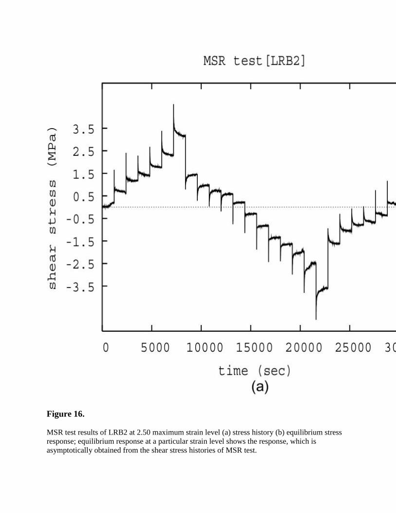
Figure 16.

MSR test results of LRB2 at 2.50 maximum strain level (a) stress history (b) equilibrium stress

response; equilibrium response at a particular strain level shows the response, which is

asymptotically obtained from the shear stress histories of MSR test.

3. Structure of the rheology model

A rheology model for describing the three phenomenological effects of the bearings as

mentioned above is constructed in this section. In Section 2, the Mullin’s softening effect, strain

rate viscosity effect, strain dependent elasto-plastic behavior with hardening effect of the

bearings are illustrated.As pointed out earlier that all the experiments were conducted on

preloaded specimens and hence the Mullin’s effect of the bearing was not considered in deriving

the rheology model. The underlying key approach of constructing the model is an additive

decomposition of the total stress response into three contributions associated with a nonlinear

elastic ground-stress, an elasto-plastic stress, and finally a viscosity induced overstress.

Thisapproach has been motivated by the experimental observations (Section 2) of the bearings

[33-35]. The decomposition can be visualized for one dimensional analogy of the rheology

model as depicted in Figure 17 (a) and (b).The model is the extended version of the Maxwell’s

model by adding two branches: one branch is the nonlinear elastic spring element and the other

one is the elastoplastic spring–slider elements.

Figure 17.

Structural configuration of the rheology model.

Motivated by the experimental observations, the mechanical behavior of the bearings can be also

described as the sum of the two different behaviors: the rate-independent and the rate-dependent

behaviors. The rate-independent behavior comprises the elasto-plastic and the nonlinear elastic

response, which are represented in the top two branches of the model (Figures 17(a) and (b)).

This phenomenon can be regarded as the equilibrium hysteresis to be identified from the relaxed

equilibrium responses of the multi-step relaxations of the bearings. On the other hand, the rate-

dependent response becomes very significant in relaxation and cyclic loading tests. The latter

showed rate-dependent hysteresis loops where the size of the hysteresis increases with the

increase of strain rates (Figures 7 (a) to (c)).

The total stress response of the bearing is motivated to decompose into three branches (Figure

17(b)):

τ=τ(γa)ep+τee(γ)+τoe(γc) (3)

Options

where τep is the stress in the first branch composed of a spring (Element A) and a slider (Element

S);τee denotes the stress in the second branch with a spring (Element B); τoe represents the stress

in the third branch comprising a spring (Element C) and a dashpot (Element D). The first and

second branches represent the rate-independent elasto-plastic behavior, while the third branch

introduces the rate-dependent viscosity behavior.

3.1. Modeling of equilibrium hysteresis

From the MSR test data (Figures 11 to 16), an equilibrium hysteresis loop with strain hardening

is visible in each bearing. This equilibrium hysteresis loop can be suitably represented by

combining the ideal elasto-plastic response (Figure 18a) and the nonlinear elastic response

(Figure 18b).

Figure 18.

Formation of equilibrium hysteresis (a) elasto-plastic response (b) nonlinear elastic response.

The elasto-plastic response as shown in Figure 18(a) can be idealized by a spring-slider element

as illustrated in Figure 19.

Figure 19.

Spring-slider model for illustrating the rate-independent elasto-plasticity.

The total strain can be split into two components:

γ=γa+γs (4)

Options

whereγa stands for the strain on the spring (Element A), referred to as the elastic part, andγs is the

strain on the slider(Element S),referred to as the plastic part.

From equilibrium consideration, the stress on the spring is τep, and we have the elastic

relationship

`

τep=C1γa (5)

Options

whereC1 is a spring constant for Element A.

The mechanical response of the slider (Element S) is characterized by the condition that the

friction slider is active only when the stress level in the slider reaches a critical shear stress

τcr,i.e., the stress τepin the slider cannot be greater in absolute value than τcrwhich can be

mathematically expressed as

{γ˙s≠0for|τep|=τcrγ˙s=0for|τep|<τcr (6)

Options

The evolution equation for the elastic strain γa can be written using the Eq.(5) as

τ˙ep=γ˙[U(γ˙)U(τcr−τa)+U(−γ˙)U(τcr+τa)] (7)

Options

with

U(x)={10:x≥0:x<0 (8)

Options

The nonlinear elastic response as shown in Figure 18(b) with strain hardening at higher strain

levels can be described by a non-Hookean nonlinear spring (Element B) (Figure 20):

τee=C2γ+C3|γ|msgn(γ) (9)

Options

whereC2, C3, and m (m> 1)are constants with

sgn(x)=⎧⎩⎨⎪⎪+10−1:::x>0x=0x<0 (10)

Options

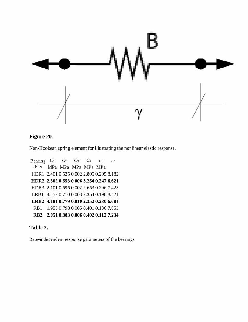
Figure 20.

Non-Hookean spring element for illustrating the nonlinear elastic response.

Bearing

/Pier

C1 C2 C3 C4 τcr m

MPa MPa MPa MPa MPa

HDR1 2.401 0.535 0.002 2.805 0.205 8.182

HDR2 2.502 0.653 0.006 3.254 0.247 6.621

HDR3 2.101 0.595 0.002 2.653 0.296 7.423

LRB1 4.252 0.710 0.003 2.354 0.190 8.421

LRB2 4.181 0.779 0.010 2.352 0.230 6.684

RB1 1.953 0.798 0.005 0.401 0.130 7.853

RB2 2.051 0.883 0.006 0.402 0.112 7.234

Table 2.

Rate-independent response parameters of the bearings

https://www.intechopen.com/source/html/38206/media/image31.jpeg

Figure 21.

Identification of equilibrium response parameters for (a) HDR2, (b) RB2, and (c) LRB2; the

experimental results are obtained from the MSR tests in asymptotic sense and the model results

are determined using τ = τee + τep with parameters given in Table 2.

In order to determine the equilibrium response parameters as presented in Eqs. (5. 6 and 9), the

equilibrium hysteresis loops as obtained from the MSR test have been considered. The

equilibrium hysteresis loops of all bearings considered in the study are presented in Figures 21

(a) to (c). The experimental data are denoted by solid circular points. The critical shear, τcris

determined by using the equilibrium hysteresis loop. The difference between loading and

unloading stresses in the equilibrium hysteresis loop at each strain level corresponds to 2τcr.

Accordingly, τcr can be determined from the half of the arithmetic average values of the stress

differences. The parameter C1 corresponding to the initial stiffness can then be determined by

fitting the initial part as well as the switching parts from loading and unloading in the

equilibrium hysteresis loop (see, for example, Figure 18(a)).Finally, the parameters for the

nonlinear spring (Element B) are identified. The subtraction of the stress τep of Eq.(5) from the

equilibrium stress response obtained from the MSR test gives the stressτee corresponding to

Eq.(9).Parameters C2, C3, and m are determined using a standard least square method. The

obtained critical stressesτcr and the equilibrium response parameters C2, C3, and m for all

specimens are given in Table 2. The equilibrium responses obtained using the proposed model

and the identified parameters are presented in Figures 21 (a) to (c). The solid line in each Figure

shows the equilibrium responses obtained by the rheology model.

3.2. Modeling of instantaneous response

At the instantaneous state, the structure of the rheology model can be reduced into the same

model without the dashpot element (Element D), because the dashpot is fixed (

γ˙d=0

) owing to infinitely high strain-rate loading. Consequently, the instantaneous response of the

rheology model can be obtained by adding τoe without Element D and the responses obtained

from the other two branches as shown in Figure 22.

Figure 22.

Spring-slider model for illustrating the instantaneous response.

https://www.intechopen.com/source/html/38206/media/image34.jpeg

Figure 23.

Identification of instantaneous response parameters for (a) HDR2, (b) RB2, and (c) LRB2; the

instantaneous response is determined using the model τ = τee + τep+ τoe(without dashpot element

D) and the experimental results represented by different lines are obtained from CS tests at four

strain rates of 0.05, 0.5, 1.5, and 5.5 /sec in loading regimes.

From the CS test results, a diminishing trend of the stress responses with increasing strain rates

can be observed in all bearings as illustrated in Figures 7 (a) to (c). From these Figures, it has

been observed that the instantaneous response lies at the neighborhood of the stress-strain curve

at a strain rate of 5.5/s for the HDRB and the LRB; however for the RB, it is around the 1.5 /s

strain rate. The instantaneous stress-strain curve, and accordingly the spring C seems to be

nonlinear even in loading regime as clearly presented in Figures 23(a) to (c).

For simplicity, a linear spring model is employed for Element C in order to reproduce the

instantaneous response of the bearings:

τoe=C4γc (11)

Options

whereC4 is the spring constant for Element C.

The parameter C4 is determined so that the instantaneous stress-strain curve calculated from the

rheology model (τ = τee+ τep+ τoe(without the dashpot element)) can envelop the stress-strain

curves obtained from the CS test. Figures 23(a) to (c) show comparison between the

instantaneous stress-strain curves from the rheology model and those from the CS test at

different strain ratesup to 5.5/s in loading regime of all bearings. The obtained parameters C4 for

all bearings are listed in Table 2.

3.3. Modeling of nonlinear viscosity

Considering the third branch of the rheology model (Figure 17), the total strain can also be

decomposed into two parts (Figure 24):

γ=γc+γd (12)

Options

whereγc and γd stand for the strains in the spring (Element C)and the dashpot (Element D),

respectively.

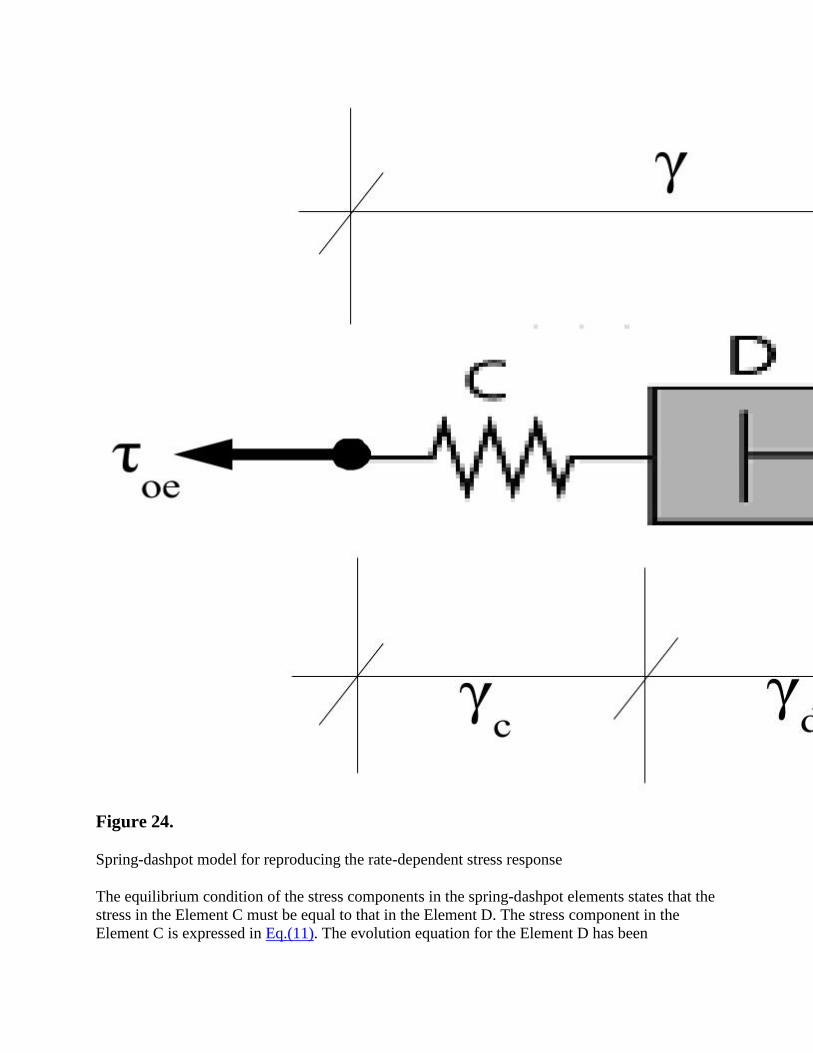
Figure 24.

Spring-dashpot model for reproducing the rate-dependent stress response

The equilibrium condition of the stress components in the spring-dashpot elements states that the

stress in the Element C must be equal to that in the Element D. The stress component in the

Element C is expressed in Eq.(11). The evolution equation for the Element D has been

constructed motivating by the experimental results of the bearings to be discussed in the

following sub-sections.This section describes the procedure to identify the constitutive

relationship of the dashpot (Element D) in the rheology model. To this end, the experimental

results obtained from the MSR and the SR tests are analyzed to derive the relationship between

the overstress τoe and the dashpot strain rate

γ˙d . A schematic diagram to identify

τoe−γ˙d

relationship is presented in Figure 25.

From the stress relaxation results of the MSR and the SR loading tests, the time histories of the

total stress τ and the total strain γ are obtained. Assuming that the asymptotic stress response at

the end of each relaxation period is the equilibrium stress τeq at a particular strain level, the over

stress history in each relaxation period is obtained by subtracting the equilibrium stress from the

total stress.Then, the time history of the elastic strain for Element C is calculated from γc= τoe/C4

in Eq.(11), and consequently the time history of the dashpot strain can be determined as γd= γ -

γcusing Eq. (12). In order to calculate the history of the dashpot strain rates, special treatment of

the experimental data is required for taking the time derivatives over the experimental data points

containing scattering due to noise. In order to reduce the scattering of experimental data, a

moving averaging technique was employed in the current scheme before taking time derivatives

of the experimental data points. All calculations were done by Mathematica[44].

https://www.intechopen.com/source/html/38206/media/image40.jpeg

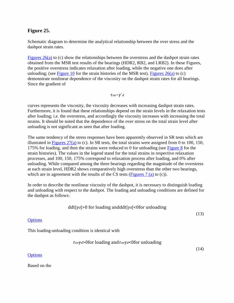
Figure 25.

Schematic diagram to determine the analytical relationship between the over stress and the

dashpot strain rates.

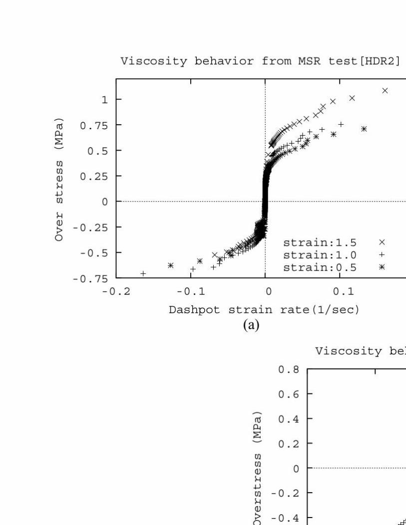
Figures 26(a) to (c) show the relationships between the overstress and the dashpot strain rates

obtained from the MSR test results of the bearings (HDR2, RB2, and LRB2). In these Figures,

the positive overstress indicates relaxation after loading, while the negative one does after

unloading; (see Figure 10 for the strain histories of the MSR test). Figures 26(a) to (c)

demonstrate nonlinear dependence of the viscosity on the dashpot strain rates for all bearings.

Since the gradient of

τoe−γ˙d

curves represents the viscosity, the viscosity decreases with increasing dashpot strain rates.

Furthermore, it is found that these relationships depend on the strain levels in the relaxation tests

after loading; i.e. the overstress, and accordingly the viscosity increases with increasing the total

strains. It should be noted that the dependence of the over stress on the total strain level after

unloading is not significant as seen that after loading.

The same tendency of the stress responses have been apparently observed in SR tests which are

illustrated in Figures 27(a) to (c). In SR tests, the total strains were assigned from 0 to 100, 150,

175% for loading, and then the strains were reduced to 0 for unloading (see Figure 8 for the

strain histories). The values in the legend stand for the total strains in respective relaxation

processes, and 100, 150, 175% correspond to relaxation process after loading, and 0% after

unloading. While compared among the three bearings regarding the magnitude of the overstress

at each strain level, HDR2 shows comparatively high overstress than the other two bearings,

which are in agreement with the results of the CS tests (Figures 7 (a) to (c)).

In order to describe the nonlinear viscosity of the dashpot, it is necessary to distinguish loading

and unloading with respect to the dashpot. The loading and unloading conditions are defined for

the dashpot as follows:

ddt|γd|>0 for loading andddt|γd|<0for unloading (13)

Options

This loading-unloading condition is identical with

τoeγd>0for loading andτoeγd<0for unloading (14)

Options

Based on the

τoe−γ˙d

relationships obtained form the MSR and the SR test data shown in Figures 26 and 27 for the

bearings, the constitutive model for the Element D can be expressed as

τoe=Alexp(q|γ|)sgn(γ˙d)∣∣∣γ˙dγ˙o∣∣∣n for loading,τoe=Ausgn(γ˙d)∣∣∣γ˙dγ˙o∣∣∣n for unloading, (15)

Options

where

γ˙o

= 1 (sec-1) is a reference strain rate of the dashpot; Al, Au,q andn are constants for nonlinear

viscosity.

In SR and MSR tests, the loading/unloading condition changes abruptly (e.g. Figures 8 to 10).

However, under general loading histories, the loading/unloading condition may change

gradually. To avoid abrupt change in viscosity due to a shift in the loading and unloading

conditions, a smooth function is introduced into the overstress expression, which facilitates the

Eq.(15a,b) to be rewritten in a more compact form

τoe=A∣∣∣γ˙dγ˙o∣∣∣nsgn(γ˙d)withA=12(Alexp(q|γ|)+Au)+12(Alexp(q|γ|)−Au)tanh(ξτoeγd) (16)

Options

whereξ is the smoothing parameter to switch viscosity between loading and unloading. Now, in

the subsequent paragraphs, the procedure for determining the viscosity constants (Al, Au,q and n)

will be discussed followed by the smoothing parameter (ξ).

Bearing

/Pier

Al Au q n ξ

MPa MPa

HDR1 0.501 0.904 0.532 0.205 1.221

HDR2 0.982 0.952 0.344 0.224 1.252

HDR3 0.754 0.753 0.353 0.213 1.242

LRB1 0.731 0.731 0.0 0.272 0.0

LRB2 0.792 0.792 0.0 0.302 0.0

RB1 0.552 0.552 0.0 0.232 0.0

RB2 0.434 0.434 0.0 0.243 0.0

Table 3.

Rate-dependent viscosity parameters of the HDRB

Using the strain histories of the SR loading tests at different strain levels (Figure 8),the

overstress-dashpot strain rates relationships are determined (Figures 27 (a) to (c)), which

correspond to Eq.16 for both loading and unloading conditions. A standard method of nonlinear

regression analysis is employed in Eq. 16 to identify the viscosity constants. As motivated by the

relationships of the overstress-dashpot strain rates obtained in the SR/MSR test results, the value

of n is kept the same in loading and unloading conditions. The nonlinear viscosity parameters

obtained in this way are presented in Table 3.Figures 27(a) to (c) present the overstress-dashpot

strain rates relationships obtained using the proposed model and the SR test results; the solid

lines show the model results and the points do for the experimental data.

A sinusoidal loading history is utilized to determine the smoothing parameter of the model

(Eq.16). The sinusoidal loading history corresponds to a horizontal shear displacement history

applied at the top of the bearing at a frequency of 0.5 Hz with amplitude of 1.75.An optimization

method based on Gauss-Newton algorithm [45] is employed to determine the smoothing

parameter. The optimization problem is mathematically defined as minimizing the error function

presented as

Minimize⎧⎩⎨E(ξ,t)=∑n=1N(τexp,n−τm,n)2⎫⎭⎬ (17)

Options

whereN represents the number of data points of interest, τexp,n and τm,n imply theshear stress

responses at time tn obtained from the experiment and the model, respectively, and ξ stands for

the parameter to be identified. Using the Gauss-Newton algorithm, following condition is

satisfied for obtaining the minimum error function as

∇E(ξi,t)+∇2E(ξi,t)(ξi+1−ξi)=0 (18)

Options

where∇ refersthe gradient operator. During the iteration process, the updated parameter in each

iteration is determined using

ξi+1=ξi−δ∇E(ξi,t)∇2E(ξi,t) (19)

Options

where δ is the numerical coefficient between 0 and 1 to satisfy the Wolfe conditions at each step

of the iteration.The values of ξ determined in this way for the bearings are presented in Table 3.

https://www.intechopen.com/source/html/38206/media/image51.jpeg

Figure 26.

Overstress-dashpot strain rate relation obtained from the MSR tests at different strain levels in

loading and unloading regimes of (a) HDR2, (b) RB2, and (c) LRB2; the values in the legend

stand for the total strain in respective relaxation processes, and 50,100, 150% correspond to

relaxation processes after loading and unloading.

https://www.intechopen.com/source/html/38206/media/image52.jpeg

Figure 27.

Identification of viscosity parameters of (a) HDR2, (b) RB2, and (c) LRB2; the model results

represented by solid lines are obtained by τ = τoe with parameters given in Table 3 and the

relations between

τoe−γ˙d

as calculated from SR test data are shown by points. The values in the legend stand for the total

strain in respective relaxation processes, and 100,150, 175% correspond to relaxation processes

after loading, and 0% after unloading.

4. Thermodynamic consistency of the rheology model

TheClausisus-Duhem inequality is a way of expressing the second law of thermodynamics used

in continuum mechanics. This inequality is particularly useful in determining whether the given

constitutive relations of material/solid are thermodynamically compatible [46]. This inequality is

a statement concerning the irreversibility of natural resources, especially when energy dissipation

is involved. The compatibility with the Clausisus-Duhem inequality is also known as the

thermodynamic consistency of solid. This consistency implies that constitutive relations of solids

are formulated so that the rate of the specific entropy production is non-negative for arbitrary

temperature and deformation processes.

In this context, the Clausius-Duhem inequality reads

−ρψ˙+τγ˙≥0 (20)

Options

where

ρ

is the mass density,

ψ

is the Helmholtz free energy per unit mass, and

τγ˙

is the stress power per unit volume.It states that the supplied stress power has to be equal or

greater than the time rate of the Helmholtz free energy.For the rheology model, the Helmholtz

free energy is the mechanical energy stored in the three springs shown in Figure17 can be

represented as

ρψ(γ,γa,γc)=12C1γ2a+12C2γ2+C3m+1|γ|m+1+12C4γ2c (21)

Options

Its time-rate reads as follows

ρψ˙(γ,γa,γc)=C1γaγ˙a+C2γγ˙+C3|γ|mγ˙+C4γcγ˙c (22)

Options

The stress power of the model is

τγ˙=(τee+τep+τoe)γ˙=τeeγ˙+τep(γ˙a+γ˙s)+τoe(γ˙c+γ˙d) (23)

Options

Inserting the stress power (Eq.24) and the time-rate of the Helmholtz free energy (Eq.23) into the

2nd law of thermodynamics (Eq. 21) and rearranging the terms leads to the following expression

(Eq.25)

(τep−C1γa)γ˙a+(τee−C2γ−C3|γ|m)γ˙+(τoe−C4γc)γ˙c+τepγ˙s+τoeγ˙d≥0 (24)

Options

In order to satisfy this inequality for arbitrary values of the strain-rates of the variables in the free

energy, the following equations for the three stress components which correspond to Eqs.(5),

(9),and (11), respectively, yield

τep=C1γa (25)

Options

The residual inequality to be satisfied is

τee=C2γ+C3|γ|msgn(γ) (26)

Options

It states that the inelastic stress-powers belonging to the two dissipative elements (Element S and

Element D) have to be non-negative for arbitrary deformation processes. Assuming that the time-

derivatives of the inelastic deformations are the same sign as the corresponding stress quantities,

each of the product terms of Eq. (27) is ensured to be non-negative with parameters given in

Table 3. The non-negative dissipation energy of the bearings is ensured only when all the

parameters responsible for expressing the elasto-plastic stress (

τoe=C4γc ) and the viscosity induced overstress (

τepγ˙s+τoeγ˙d≥0

) are non-negative. The parameters of Table 3 have confirmed this condition.

5. Summary

This chapter discusses an experimental scheme to characterize the mechanical behavior of three

types of bearings and subsequently demonstrates the modeling approaches of the stress responses

identified from the experiments. The mechanical tests conducted under horizontal shear

displacement along with a constant vertical compressive load demonstrated the existence of

Mullins’ softening effect in all the bearing specimens. However, with the passage of time a

recovery of the softening effect was observed. A preloading sequence had been applied before

actual tests were carried out to remove the Mullins’ effect from other inelastic phenomena.

Cyclic shear tests carried out at different strain rates gave an image of the significant strain-rate

dependent hysteresis property. The strain-rate dependent property in the loading paths was

appeared to be reasonably stronger than in the unloading paths. The simple and multi-step

relaxation tests at different strain levels were carried out to investigate the viscosity property in

the loading and unloading paths of the bearings. Moreover, in order to identify the equilibrium

hysteresis, the multi-step relaxation tests were carried out with different maximum strain levels.

The dependence of the equilibrium hysteresis on the experienced maximum strain and the

current strain levels was clearly demonstrated in the test results.

The mechanical tests indicated the presence of strain-rate dependent hysteresis with high strain

hardening features at high strain levels in the HDRB. In the other bearing specimens, strain-rate

dependent phenomenon was seen less prominent; however, the strain hardening features at high

strain levels in the RB showed more significant than any other bearings. In this context, an

elasto-plastic model was proposed for describing strain hardening features along with

equilibrium hysteresis of the RB, LRB and HDRB. The performance of the proposed model in

representing the strain rate-independent responses of the bearings was evaluated.In order to

model the strain-rate dependent hysteresis observed in the experiments, an evolution equation

based on viscosity induced overstress was proposed for the bearings. In doing so, the Maxwell’s

dashpot-spring model was employed in which a nonlinear viscosity law is incorporated. The

nonlinear viscosity law of the bearings was deduced from the experimental results of MSR and

SR loading tests. The performance of the proposed evolution equation in representing the rate-

dependent responses of the bearings was evaluated using the relaxation loading tests.

On the basis of the physical interpretation of the strain-rate dependent hysteresis along with other

inelastic properties observed in the bearings, a chronological method comprising of

experimentation and computation was proposed to identify the constitutive parameters of the

model. The strain-rate independent equilibrium response of the bearing was identified using the

multi-step relaxation tests. After identifying this response, the elasto-plastic model (the top two

branches of the rheology model) was used to find out the parameters for the elasto-plastic

response. A series of cyclic shear tests were utilized to estimate the strain-rate independent

instantaneous response of the bearings. A linear elastic spring element along with the elasto-

plastic rheology model (the rheology model without the dashpot element) was used to determine

the parameters of the instantaneous responses. After determining the elasto-plastic parameters of

the bearings, the proposed evolution equation based on the viscosity induced overstress was used

to find out the viscosity parameters by comparing the simple relaxation test data. Moreover, a

mathematical equation involving smoothing function was proposed to establish loading and

unloading conditions of the overstress; and sinusoidal loading data was then used to estimate the

smoothing parameter of the overstress. Finally, the thermodynamic compatibility was confirmed

by expressing the rheology model by using the Clausius-Duhem inequality equation.

Acknowledgement

The experimental works were conducted by utilizing the laboratory facilities and bearings-

specimens provided by Rubber Bearing Association, Japan. The authors indeed gratefully

acknowledge the kind cooperation extended by them. The authors also sincerely acknowledge

the funding provided by the Japanese Ministry of Education, Science, Sports and Culture

(MEXT) as Grant-in-Aid for scientific research to carry out this research work.