Credible Capacity Preemption in a Duopoly Market under

Uncertainty

Jianjun Wu∗

University of Arizona

February 14, 2006

Abstract

This paper explores firms’ incentives to engage in capacity preemption using a continuous-time

real options game. Two ex ante identical firms can choose capacity and investment timing regarding

the entry into a new industry whose demand grows until an unknown maturity date, after which it

declines until it disappears. Previous literature usually predicts that the Stackelberg leader, whether

endogenously or exogenously determined, is better off by building a larger capacity than its rival. In

contrast, this paper proves that, under certain conditions about the demand function and the market

growth rate, in equilibrium the first mover enters with a smaller capacity. If it had chosen the larger

capacity, its competitor could, and in fact would use a smaller plant to force it out of the market.

The result is driven by two facts: first, the large capacity firm lacks the incentive to preempt its

competitor, because of its higher option value, which tends to delay its investment; second, the large

firm also lacks commitment to fight for the market if its leadership is challenged by a smaller firm,

because the smaller firm can credibly commit to stay in the market.

∗Department of Economics, The University of Arizona, Tucson, AZ 85721-0108. E-mail: jjwu@eller.arizona.edu. I amvery grateful to David Besanko and Mark Satterthwaite for numerous helpful conversations and precious encouragementthroughout this project. I also want to thank James Dana, David Dranove, Martin Dufwenberg, Peter Eso, Yuk-Fai Fong,Francisco Ruiz-Aliseda, Rakesh Vohra, and seminar participants at the University of Arizona, UC Davis, and NorthwesternUniversity for their valuable comments.

1

1 Introduction

Theoretical industrial organization models have long recognized the value of first mover advantage

regarding the timing of entry, which can be traced back as early as von Stackelberg (1934) . By investing

in a larger capacity ahead of its competitor, a firm can achieve higher profit than its follower1. Further,

if firms are competing for the leadership in a market with uncertainty, making an earlier capacity

commitment enables a firm to obtain Stackelberg leadership. In this case, the follower enjoys the value

of flexibility, but its profit is generally lower than the leader. (Sadanand and Sadanand (1996), and

Maggi (1996))

In real business world, however, we rarely observe leading firms engaging in large capacity pre-

emption. In contrast, there are many cases in which either firms failed or deliberately gave up the

opportunity to preempt their competitors with a large capacity. In the titanium dioxide industry, Du

Pont chose not to expand its capacity to preempt its competitor, Ker McGee, even it seemed fairly

reasonable2; In the digital video recorder (DVR) industry, Motorola decided not to produce DVR inte-

grated set-top box until two years after the entry of its smaller competitor, Scientific Atlanta3; Finally

in hot spot industry, Cometa Networks, a joint venture initiated by Intel, IBM, and AT&T as an ac-

claimed would-be industry leader in providing nation-wide wireless hot spot service, not only failed to

preempt its competitor, T-mobile, but also failed to contest the first mover’s leadership with a more

ambitious network4.

The difference between the theoretical prediction and business practice raises the question of why first

entrants refrain from engaging in large capacity preemption while the advantages seem so compelling in

theory. One probable reason is that the literature has focused on the cases in which uncertainty either

does not exist or will be resolved immediately after the entry of the leader. Little is known in the case

where the leader has to enter a developing market with evolving uncertainty. By introducing a new

continuous-time real option game of timing, this article proves that under fairly general conditions about

market demand, the leader would rather enter the market with a smaller capacity than its follower’s.

The reason is that to secure its market leadership, the leader not only needs to move ahead of its

1See Gal-Or (1985). Tirole (1988) also has nice discussion of Stackelberg leadership.2See Ghematwat (1984) . This has become a classical case to teach preemption to MBA students in many US business

schools and the irony is that it turned out Du Pont chose not to preempt.3See "Mototrola gets a digtal-video black eye." Wall Street Journal, April 15, 2004.4See "Chill hits Hot Spots." Wall Street Journal, March 18, 2004.

2

competitor but also needs a credible commitment to stay in the market. Sinking a large amount of

investment alone does not commit the leader to fight for the market. In fact, when a war of attrition

broke out in a premature market, the large leader would have more incentive to abandon the market

than its smaller follower. As a result, the leader in fact would enter the market with a smaller capacity.

The underlying driving force of this result lies in the evolving market uncertainty, which is modeled

as an unknown market switching date. The market is originally growing but will switch to decline after a

random date. The risk of sudden downturn creates an option value of delaying investment, as predicted

by literature on investment uncertainty5. The difference, however, is that in the competition for market

leadership, this option value confers a strategic advantage to the smaller firm: it enables the smaller

firm to win the war of attrition in the growing market. The intuitions are as follows: first, as shown

in Ghemawat and Nalebuff (1985), in the declining market a larger firm will exit earlier and leaving

the smaller firm to monopolize the market. As a result, the smaller firm has more to lose if it exits

the market earlier when the market is growing, which in turn strengthens the smaller firm’s incentive

to fight for the market. Consequently, large capacity preemption is not credible because rather than

delaying the entry of the follower, it in effect would invite the smaller follower to jump into the market

earlier to challenge the first mover’s leadership and eventually force the larger leader out of the market

by starting a war of attrition.

This paper is directly related to the literature on endogenous Stackelberg leadership. Most previous

papers, however, understates the effect of market uncertainty on firms’ strategic incentive to preempt

by limiting the negative effect of adverse market outcomes. For example, Maggi (1996) assumes that the

lower bound of the demand be large enough that a Cournot duopoly will never abandon the market in the

second stage. In contrast, additional insights are provided by this paper, which focuses on modeling this

situation by considering a market with unknown switching date. Unlike previous studies, the premature

market switching to downturn will result in a loss on the incumbents if the market changes to decline

prematurely. With this framework, the "bad news principle of irreversible investment" is applied to a

game theoretic setup: the strategic effect of option value completely changes the predictions on a firm’s

equilibrium capacity and entry timing choices as stated in the previous papers.6

5See Dixit and Pindyck (1994) for an excellent survey.6"Bad news principle of irreversible investment" was proposed by Bernanke (1983), which implies that only bad future

market outcome matters in whether one should make irreversible investment today. See Ruiz-Aliseda and Wu (2004) fordetail discussions.

3

It is also worth noting that most existing papers employ a two-stage model to explain the endogenous

asynchronous entry of two firms into a new market, based on extended game with observable delay

proposed by Hamilton and Slutzsky (1990) 7. Maggi (1996) is the first paper to allow firms to choose

capacity and entry timing simultaneously by dividing the game into a pre-commitment and a production

stage. Because no production is allowed in the pre-commitment stage, in equilibrium only one firm

becomes the de facto leader by making capacity commitment in the first stage, leaving the other firm

to enter at the beginning of the second stage. As a result, the leadership race is reduced to a lottery

on who gets to move in the first stage. By considering a continuous-time model, this paper allows firms

to compete for the market leadership in a more realistic sense. Further, the paper shows that the first

mover’s advantage will vanish if firms are competing for the leadership in an emerging market where

immediate large capacity investment is not feasible.

This paper is divided into seven sections. We start laying out the model in Section 2 and discuss

a benchmark monopoly model in section 3. Section 4 and 5 solve the duopoly game of entry and exit.

Section 6 explores possible relaxations of the assumptions and section 7 concludes the paper. Most

proofs are presented in the Appendix.

2 Model

Consider a continuous-time game of entry and exit over the lifetime of a new industry with two ex

ante identical firms.8 As analyzed by Simon and Sinchcombe(1986) , the game of continuous time

is modeled as the limit of discrete time as period length goes to zero. Each firm can select its own

capacity level and entry timing. The investment cost is I per unit of capacity. Once a firm sinks its

investment cost, it can operate immediately and the operating cost is c per unit of capacity. Firms are

free to exit the market at any time. Moreover, after exiting the market, a firm is allowed to restart

its plant later by incuring the full investment cost again.9 Specifically, let K = {0, q1, q2, ..., qn} with7The main limitation of this model is that it separates firms capacity and entry timing decisions by requiring firms to

announce their entry timing before making capacity choices. See, for example, Sadanand and Sadanand (1996) , and vanDamme and Hurkens (1999) and Hirokawa and Sasaki (2001)

8 In this paper, we restrict the analysis to two potential entrants for several reasons: first, duopoly analysis is the firststep to understand the strategic interaction in an oligopoly market. second, it is still a difficult problem to analyze firms’strategic investment in a real options framework, even if there are only two firms. Third, Fudenberg and Tirole (1985)shows that preemption games with three or more players usually involve more complexities since the rent equalizationprinciple may not apply in all subgames.

9Restarting some technologies, such as Aluminum oxide, is not easy and will incur significant cost, as shown inWells(1985) . One key assumption for modeling continuous-time game as the limit of discrete time game is not to al-

4

0 < q1 < q2 < ... < qn denote a firm’s possible plant sizes. At each date t ≥ 0, firm i (i = 1, 2) can

choose a capacity level κi from its action set Ki, where Ki depends on whether the firm has invested

before t. By choosing κi = 0, it will continue to stay out of the market, otherwise it can choose from n

discrete capacity levels. If it has already been producing in the market or has entered the market before

with capacity κ (∈ {q1, q2, ..., qn}) , its action set is limited to Ki = {0, κ} .Action 0 means to exit themarket immediately at t and κ means to stay in the market. In this paper, I assume that a firm cannot

change its chosen capacity levels.10

Let Q = κ1 + κ2 denote the total capacity active in the market. As in Ghemawat and Nalebuff

(1985) and Londregan (1990) , I assume that the firms produce at full capacity and sell all their output

when active in the market.11 This assumption also enables the model to focus on a firm’s entry and

exit decisions by avoiding the complicated discussion of capacity constrained competition. As a result,

the short term market supply is inelastic, and the equilibrium price will vary only with demand shocks.

Following Dixit and Pindyck (1994), the market price is determined by the product of two factors:

P (Y,Q) = Y D (Q) . (1)

D (·) is a decreasing function of Q, which implies that the larger the total capacity of the active firmsthe lower the price. The lumpiness of capacity investment and disinvestment implies that adding or

withdrawing capacity will result in a downward or upward jump of market price. The market price is

also affected by a random demand shock represented by Y. To be concrete, Y represents the potential

market demand, which is meant to capture the effect that the larger the size of the potential market,

the higher the price given the fixed supply. The initial market size for this new product is Y = y0, which

grows exponentially over time at the rate of α1. To introduce uncertainty, I assume that the market

growth stops at an unknown date τ that is exponentially distributed with the parameter λ and density

function f (τ) = λe−λτ . Once the market stops growing, Y switches to decline at the rate of α2 < 0 from

low firms to exit and reentry infinite times. Costly reentry combined boundedness of a firm’s financial resources aresufficient. See Simon and Stinchcombe(1986) for more details.10This is for the simplicity of the model. It has two implications: first, firms are not allowed to expand or shrink its

capacity during operation, otherwise the model becomes very complicated. Further, a more stringent implication is that italso implies that a firm cannot change its capacity during its reentry. Excluding this possibily allow us to focus on firms’initial entry capacity, which is also the central issue on capacity preemption and competition for Stackelberg leadership.11 In reality many firms, for example automakers, would rather reduce the selling price to keep the plant operating at

full capacity (Mackintosh 2003). Also, due to the uncertainty of the market, firms might get stuck with their labor andraw material supply contract, which makes capacity shrinkage extremely difficult.

5

Y (τ) , the level reached at the end of growing stage, until it disappears. In other words, the process

of Y is evolving continuously except that there is a change of direction from growth to decline once τ

is resolved. This uncertainty setup is different from that in previous papers on endogenous leadership,

which usually assume that the demand realization could be high or low at a specific date known to both

firms. In contrast, I assume that no firm knows how long the market growth will last. The switching

of market demand from growth to decline is bad news to firms in the market. The uncertainty of this

market switching creates option value and one main purpose of this paper is to study the effect of this

"bad news" on firms’ strategic investment behavior.12

Since firms are ex ante identical, either firm could become the leader. Hence I will only discuss

the equilibrium in terms of leader’s and follower’s strategy without direct reference to their identity.

However, one common issue of the continuous timing game is the coordination regarding players’ making

simultaneous move. I follow Dutta, Lach and Rustichini (1995) , Grenadier (1996) and Weeds(2002) to

make the following assumption to rule out ex post simultaneous entry:13

Assumption 1 If both firms attempt to enter the market at the same date t, then only one of two firms

will succeed and in this case, the probability of firm 1 entering first is p = 12 .

Once the market switches to decline, the demand will decrease continuously and ultimately cause

the market price to fall below operating cost. Ghemawat and Nalebuff (1985) shows that there is a

continuum of equilibria when both firms are the same size. The following assumption is introduced as

a tie breaking rule14:

Assumption 2 After the market switches, firm i0s capacity is randomly reduced by δi where δi is

uniformly distributed on£0, δ¤, where δ is small. The realization of δ0is are common knowledge to both

firms.12As mentioned by Bernanke (1983) , firms’ benefit from delaying investment comes from the avoidance of possible loss

due to the occurrence of an unfavorable event, which he calls the "Bad News Principle of Irreversible Investment". Mypaper studies the linkage of this principle with firm’s strategic capacity choice.13This assumption might be the result of some institutional features; for example, to make the investment, the firms

need to obtain a license, and the business license office randomly picks one of two firms to award the license at a time.This assumption can also be the result of random delay in the execution of investment decisions. For example, it can beimplemented by the following mechanism: if two firms select the same entry timing t, their actual entry timing is actuallyt+ z, where z ∈ [0, ε] with ε small. Therefore, ex post, one firm always sees its competitor entering first. In this case, afterupdating its information immediately, it can choose to enter anyway to contest the first entrant’s market leadership or towait for its optimal entry date as a follower.14Without this tie-breaking rule, I have to introduce mixed strategy equilibrium. It can be shown that as long as firms

employ symmetric mixed strategy, the result of the paper still hold. So this assumption is for the simplicity of the paper.See Wu(2005) for more details.

6

This assumption is used to purify the equilibria when firms are of the same sizes so that we can clearly

characterize their equilibrium payoff in the declining stage.

Finally, I also assumeR∞0 f (τ) (y0e

α1sD (κ)− c)κe−rsds <∞, for all κ = q1, q2, ..., qn, which is used

to guarantee the integrability of firm’s expected payoff.15 A sufficient condition for this is r > α1 − λ.

In this paper, I employ the solution concept of (pure strategy) Markov perfect equilibrium, which

restrict the analysis to those strategies as a function of its payoff relevant state. The payoff relevant

state is defined by an array of variables: ht =©κ1t , κ

2t , ω

ª, where t is the current date, κit denotes firm

i0s capacity at date t, and ω denotes whether the market has switched or not.

Numerically it is not difficult to derive the equilibrium of the above general model. In fact, a

computed example is presented in Section 6. However, it is a daunting task to give an analytic solution

to the model without further assumptions. Therefore, in the following discussion, I will introduce some

simplifying assumptions and relax those assumption in Section 6. First, since the main question of this

paper is whether a firm will be able to preempt its competitor credibly by choosing a larger capacity, it

is sufficient to consider the case of two choices of plant sizes:

Assumption 3 Firms can choose two sizes of plants: small (S) or large (L) , with S < L.

As above-mentioned, market switching from growth to decline means "bad news" for firms, because

a firm’s expected profit will decrease even if the demand is evolving continuously. Ruiz-Aliseda and

Wu (2004) proves that even we allow demand Y to evolve continuously, there is still a value jumping

down at the date when market switches. The following assumption further emphasize the risk of market

switching by introducing a possible market crash at the switching date:

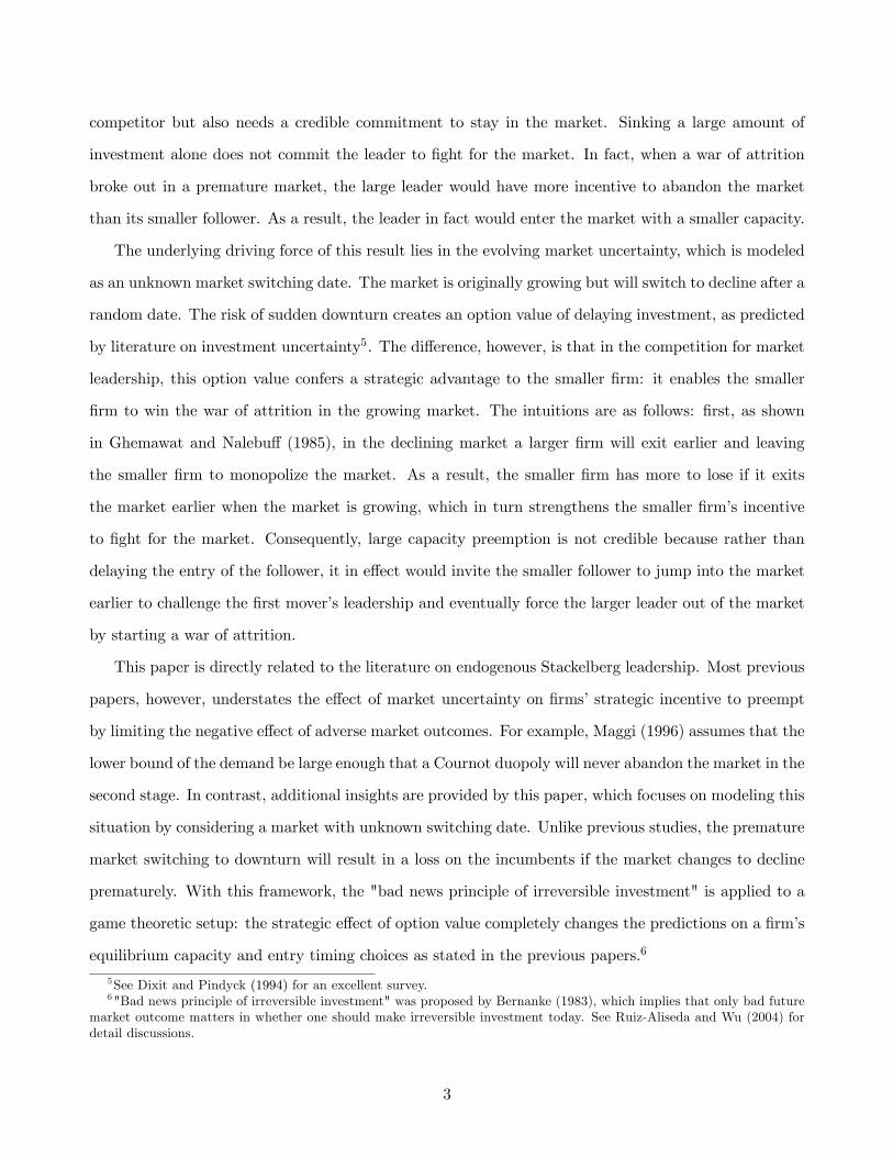
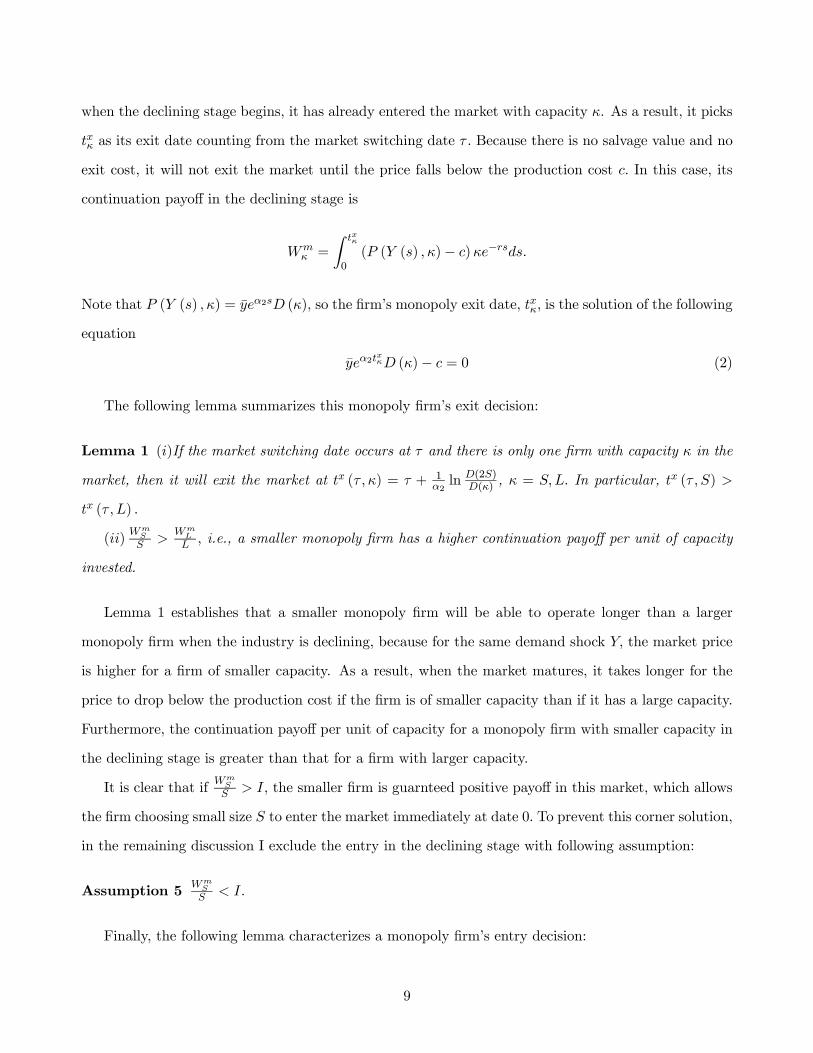
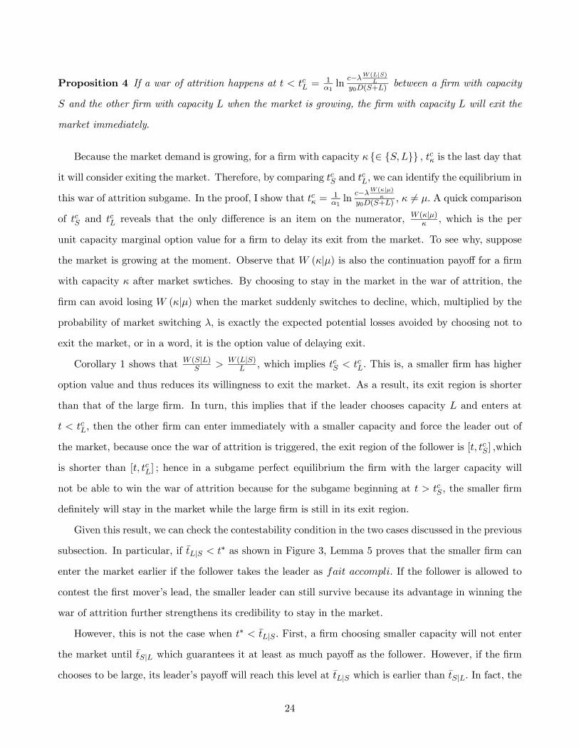
Assumption 4 L ≤ 2S and the declining stage starts with demand level Y = y, where y = cD(2S) .

This assumption implies that once the declining stage starts, there is no room for two firms since

the declining stage will start with a demand level y such that P (y, 2S)−c = 0. Figure 1 shows a samplepath of market evolution given this assumption, which implies that the continuation payoff associated

to a declining industry is not contingent on the realization of a market switching date. However, the

date τ at which this continuation payoff is realized is still uncertain. This assumption facilitates the

tractability of the model, which allow us to provide an analytical solution of the model.16

15Note that this integral is the expected payoff in the growing stage for a monopoly firm that invests at date 0.16This assumption simply divides the process of market evolution into two independent processes. As a result, there is

7

τt

Y

y0

y

Figure 1: A sample path of market evolution

Before solving the model, let me define some notations. First, L (t, μ|κ) denotes the leader’s expectedpayoff when it chooses capacity μ to enter at date t and the follower selects capacity κ. F (t, κ|μ) isdefined similarly as the follower’s payoff with capacity κ while the leader chooses μ. Also, let M (t, κ)

represent the expected payoff for a monopoly firm with capacity κ entering at t17. On the other hand,

I use t and t to denote the leader’s and follower’s entry dates, respectively. Similarly, tμ|κ denotes the

entry time for a leader with capacity μ when its follower chooses capacity κ, and tκ|μ represents the

entry date of a follower with capacity κ when the leader picks capacity μ. Similarly, the monopoly entry

date for a firm with capacity κ is denoted as tmκ . Finally, proofs are presented in the appendix if not in

the main text.

3 Monopoly Entry and Exit Decisions

I first present some results regarding a monopoly firm’s entry and exit decisions in this market, which

provides a benchmark case that is useful for later discussions. This case also introduces the concept of

marginal option value, which is a critical concept that affects a firm’s investing behavior in this paper.

Consider a firm owning a monopoly right to invest in this new market. Since the market ultimately

will switch to decline, it is natural to start with its exit decisions in the declining stage. Suppose that

also a possibility that the process might jump up if Y switches before it reaches y. Actually for large enough investmentcost, firms will not invest before Y reaches y. Although there is a loss of generality with this assumption, it helps us topresent some important results of market structure, which is not possible unless we resort to numerical methods.17Note that M (t, κ) = L (t, κ|0) = F (t, κ|0) , because monopoly can be consider as a special case when your competitor

choose not to enter the market.

8

when the declining stage begins, it has already entered the market with capacity κ. As a result, it picks

txκ as its exit date counting from the market switching date τ . Because there is no salvage value and no

exit cost, it will not exit the market until the price falls below the production cost c. In this case, its

continuation payoff in the declining stage is

Wmκ =

Z txκ

0(P (Y (s) , κ)− c)κe−rsds.

Note that P (Y (s) , κ) = yeα2sD (κ), so the firm’s monopoly exit date, txκ, is the solution of the following

equation

yeα2txκD (κ)− c = 0 (2)

The following lemma summarizes this monopoly firm’s exit decision:

Lemma 1 (i)If the market switching date occurs at τ and there is only one firm with capacity κ in the

market, then it will exit the market at tx (τ , κ) = τ + 1α2ln D(2S)

D(κ) , κ = S,L. In particular, tx (τ , S) >

tx (τ , L) .

(ii)WmSS >

WmLL , i.e., a smaller monopoly firm has a higher continuation payoff per unit of capacity

invested.

Lemma 1 establishes that a smaller monopoly firm will be able to operate longer than a larger

monopoly firm when the industry is declining, because for the same demand shock Y, the market price

is higher for a firm of smaller capacity. As a result, when the market matures, it takes longer for the

price to drop below the production cost if the firm is of smaller capacity than if it has a large capacity.

Furthermore, the continuation payoff per unit of capacity for a monopoly firm with smaller capacity in

the declining stage is greater than that for a firm with larger capacity.

It is clear that if WmSS > I, the smaller firm is guarnteed positive payoff in this market, which allows

the firm choosing small size S to enter the market immediately at date 0. To prevent this corner solution,

in the remaining discussion I exclude the entry in the declining stage with following assumption:

Assumption 5 WmSS < I.

Finally, the following lemma characterizes a monopoly firm’s entry decision:

9

Lemma 2 (i) A firm with capacity κ will choose to enter the market at tmκ , where tmκ satisfies

P (Y (tmκ ) , κ)− c = rI + λ

µ−W

mκ − Iκ

κ

¶(3)

(ii) tmS < tmL .

The monopoly firm is able to pick its entry date according to a rule of marginal cost equal to

marginal revenue. The left hand side of Equation (3) is the marginal cost of waiting to invest, which

is the instantaneous profit per unit of capacity lost by staying out. The right hand side represents

the marginal value of waiting, which consists of two parts: rI is the per unit investment cost saved

by delaying entry into the market and λ³−Wm

κ −Iκκ

´is the marginal option value of waiting. To see

why, observe that for each instant, there is probability λ that the market switches to decline, the

occurrence of which will result in a continuation payoff of Wmκ for the monopoly firm with capacity κ.

By our assumption, Wmκ − Iκ is negative, which implies that the firm will incur a loss when the market

switches. However, if the firm delays investment by one instant, it will be able to avoid this loss by

staying out of the market because once the market switches it will stay out of the market forever with

a payoff of zero. As a result, this potential loss avoided multiplied by the probability of occurrence λ is

exactly the marginal option value of waiting. Given this entry timing rule, a monopoly firm will pick

the capacity level that generates highest expected payoff and enter the market at the optimal entry date

specified by Lemma 2.

4 Duopoly exit in the declining industry

In the previous section, I discussed a benchmark case with only one entrant, in which this firm chooses

an optimal entry date that equals the marginal cost to marginal value of investment. In particular, the

marginal value of investment consists an option value component, which tends to delay entry. In the

next three sections, I will extend this framework to the duopoly case, with the purpose to study the

effect of this marginal option value on firms’ strategic entry behavior.

Depending on whether the market has matured or not, the model is naturally divided into two

phases, the growing industry and the declining industry. As a result, I solve the game backwards and

start with the declining industry.

10

Suppose the market has switched from growth to decline. There are two cases to consider: monopoly

and duopoly. The monopoly case is the one when the second firm did not enter the market before market

switches. In this case, because there is only one firm in the market, it will exit the market at its monopoly

exit date as derived in Lemma 1 since the other firm will not enter the declining market. If both firms

are in operation before the decline begins, each firm will have to choose its exit date because the industry

will ultimately become unprofitable. Depending on whether the firms are the same size or not, there are

two cases to consider. The following proposition characterizes the perfect equilibrium of this subgame

based on the sizes of the two firms.

Proposition 1 Suppose there are two firms in operation when the market switches at date τ ,

(i) if the firms are of different sizes, the larger firm will exit immediately at date τ while the smaller

firm will exit at its monopoly exit date tx (τ , S).

(ii)if both firms are of the same size, as δ → 0, one firm will exit the market immediately and the

other firm will stop operation at its monopoly exit date.

When firms are asymmetric, it is always the larger firm that exit market first, which is a well-known

result first presented in Ghemawat and Nalebuff (1985). No firm is willing to operate at a loss once the

declining industry starts, while at the same time, each firm wants its competitor to leave the market

so that it can stay until its monopoly exit date. If the firms’ sizes are different, the smaller firm has

a credible threat to outlast the larger firm because as a monopoly, the smaller firm can operate longer

than the larger firm by Lemma 1. Realizing this, in a subgame perfect equilibrium, the larger firm

had better exit the market at the duopoly exit date to avoid any losses. By Assumption 4, once the

declining industry starts, there is no room for the coexistence of two firms, hence the larger firm will

exit immediately once the market matures.

However, if both firms have the same capacity, Assumption 2 introduces a perturbation of the firms’

sizes by randomly shrinking each firm’s capacity by a small amount. As discussed in Ghemawat and

Nalebuff (1985) , this purturbation will purify continuum of mixed strategy equilibrium. As a result, ex

post one firm always realizes that it will never be able to outlast the other firm in the war of attrition,

and thus it is in its best interest to leave the market immediately. The following corollary characterize

firms’ continuation payoff in the declining stage:18

18Note that in the declining stage, the firms’ sizes are slightly different from their entry sizes as a result of the random

11

Corollary 1 If two firms with different sizes are in the market when the declining stage starts, let

W (κ|μ) denote the continuation payoff of a firm with capacity κ if its competitor has capacity μ. Thus,

W (L|S) = 0

W (S|L) =

Z txS

0(yeα2sD (S)− c)Se−rsds =Wm

S

If the declining stage starts with two firms of the same size,

W (L|L) =1

2Wm

L , if both firms are of size L

W (S|S) =1

2Wm

S , if both firms are of size S.

Assumption 2 is actually a tie breaking rule. Without this assumption, there is a continuum of

mixed strategy equilibria as shown by Ghemawat and Nalebuff (1985) , one of which is the symmetric

mixed strategy equilibrium in which two firms each choose a distribution of exit dates between market

maturity date and monopoly exit date and the choice of this distribution will completely dissipates

the rent of all future possible monopoly profits because firms must be indifferent between staying and

exiting.19

5 Duopoly entry in the growing industry

Given firms’ exit strategy in the declining stage, we can analyze firms’ entry strategies in the growing

industry. By Assumption 5, the expected profit from the declining stage alone is not enough to cover

the investment cost, which implies entry only occur before market switches. Because two firms are ex

ante identical, either firm could preempt the other. Once a firm observes the entry of its competitor

before it makes any move, it has two choices: either accepts its position as the follower or jumps into

the market to contest the first entrant’s leadership by forcing it out of the market. In previous studies of

endogenous leadership, leader never concerns the possibility of being forced out by the follower because

capacity reduction of δ0is. However, I assume δ to be small so that the payoff change due to this slight size change isignored. Thus I abuse the notation here by ignoring the small changes of firms’ continuation payoff due to the tiny randomshrinkage of firms’ sizes.19See Anderson, Goeree and Holt (1998) , Fudenberg and Tirole (1986) . In fact, without Assumption 2, the results of

this paper still hold if we require firms to choose this symmetric mixed strategy equilibrium in the decline phase. Further,there many asymmetric equilibria but in this paper, I will not consider those asymmetric equilibria because it will giveone firm ex ante advantage in the declining stage.

12

competition for market leadership ends when one firm enters the market. By allowing the follower

contest the first entrant’s leadership, I divide the analysis of firms’ entry behavior into three steps.

First, I assume that the follower takes the entry of the leader as a fait accompli, which means that

it does not try to contest the leader’s position. With this assumption, I analyze the follower’s entry

decision given the leader’s capacity and entry timing choice. Then I proceed to analyze of leader’s best

choice of size and entry date given the prediction of follower’s best response, which will identify the

potential equilibrium. Finally, I check whether the leader’s strategy is indeed immune to the possible

contest by a follower in this equilibrium.

5.1 Optimal entry date as a follower

Suppose the current date is t0 and one firm has already entered the market with capacity μ. If the

follower chooses capacity κ to enter the market at t ≥ t0, it will achieve the following expected payoff,

which is discounted back to date 0 :

F (t, κ|μ) =Z ∞

tf (τ)

⎛⎜⎝ R τt [P (Y (s) , μ+ κ)− c]κe−rsds

+e−rτW (κ|μ)− Iκe−rt

⎞⎟⎠ dτ . (4)

Note that the follower will be able to enter the market if and only if the market switching date τ is

later than the entry date t chosen by the follower. In particular, the follower’s value function consists

of three parts:R τt [P (Y, μ+ κ)− c]κe−rsds is the expected discounted profit from the duopoly growing

market until the maturity date. The second part, e−rτW (κ|μ), is the discounted continuation payoffassociated with the declining stage, and the third part Iκe−rt is the total investment cost properly

discounted.

Given the leader’s capacity choice, if the follower selects capacity κ, the following proposition gives

its best entry timing.

Proposition 2 Let t0 be the current date and the leader has entered the market with capacity κ.If the

follower chooses capacity κ, taking the leader’s position as fait accompli, then it will enter the market

at date is tκ|μ = max©t0, t

fª, where tf satisfies

PhY³tf´, μ+ κ

i− c = rI + λ

µ−W (κ|μ)− Iκ

κ

¶(5)

13

The follower’s entry decision rule is similar to that of a monopoly firm discussed in Section 3 except

that the firm is a duopoly now. The left hand side of Equation (5) is the marginal cost of waiting

to invest, which is the instantaneous profit per unit of capacity. The right hand side represents the

marginal value of waiting to invest, consisting of two parts: rI is the per-unit investment cost saved

by delaying entry into the market, and the second part is the marginal option value of waiting. For

each instant there is probability λ that the market switches to decline, which will render a payoff of

W (κ|μ)κ per unit of capacity and it is smaller than per unit cost of investment I. Hence −

³W (κ|μ)

κ − I´

is positive and represents the loss avoided in the event that the market suddenly begins to decline. As

a result, this potential loss avoided multiplied by λ, the probability of market switching in the next

instant, becomes the marginal option value of waiting.20

Define φ (κ|μ) = −λ³W (κ|μ)

κ − I´, which is the marginal option value per unit of capacity for a

firm choosing κ while its competitor selects capacity μ. The following corollary shows a relationship of

follower’s optimal entry date in two cases where the resulting duopoly market structure is the same.

Corollary 2 tS|L ≤ tL|S , i.e., if the leader chooses large capacity and the follower chooses small capac-

ity, the follower delays its investment less than if the leader chooses a small capacity and the follower

chooses a large capacity.

Proof. Since φ (L|S) > φ (S|L) , we must have

tS|L =1

α1ln

rI + c+ φ (S|L)y0D (L+ S)

<1

α1ln

rI + c+ φ (L|S)y0D (S + L)

= tL|S

When the resulting duopoly market structure is the same: one large firm and one small firm, the

option value effect is the sole driving force in the difference in entry timing. In particular, when the

follower chooses smaller capacity, it can enter the market earlier than if it chooses the larger capacity

to enter the market. This implies that in this uncertain, large capacity preemption might achieve just

the opposite: inviting the follower coming into the market earlier, even if the follower has no intension

to contest the first entrant’s leadership. The smaller option value of waiting for the smaller firm gives

20Note that this formula is actually the option value of waiting on the per unit capacity basis, which is obtained bydividing total loss avoided by the capacity level. Also, the monopoly entry date tmκ derived in Lemma 2 is actually a specialcase of tκ|μ, as if the leader selects capacity μ = 0.

14

it more incentive to invest earlier. This will have an effect on leader’s entry capacity choice. Before

moving on the analysis on the leader’s entry strategy, I first summarize the follower’s optimal strategy.

Given the follower’s optimal entry timing, we are ready to study its optimal capacity choice. It turns

out that given the leader’s capacity choice of μ, the follower’s optimal capacity choice depends on a

threshold αμ =(λ+r)[lnD(μ+S)−lnD(μ+L)−ln ημ]

lnL−lnS−ln ημ , where ημ = rI+c+λφ(S|μ)rI+c+λφ(L|μ) < 1 and μ = S,L. In fact, ημ

can be viewed as an option value factor, because it compares the investment cost with the incorporated

marginal option value being the sole difference. In particular, if the market growth rate is α1 < αμ, the

follower will choose small capacity S; otherwise it will select large capacity L if α1 ≥ αμ. The relationship

between αS and αL is generally ambiguous without the further assumption about the demand function

D (Q). The following lemma gives a sufficient conditions for αS < αL when the demand is linear21:

Lemma 3 Let D (Q) = a− bQ. If 2L+ S > ab > 2S + L, then αS < αL.

In the following discussions, I will concentrate on the case of αS < αL, because in this case the threshold

of choosing a large capacity is higher when the leader engage is larger, which is consistent with previous

literature in the sense that large Stackelberg leader induce the follower to smaller.

Proposition 3 Let the current date be t0 < tmS and suppose αS < αL. Given Assumptions 1-5, if

α1 ≤ αS , then the follower has a dominant strategy to choose small capacity. If αL > α1 > αS , the

follower will choose a capacity level different from the leader’s choice. If α1 > αL, the follower will

always choose large capacity.

Proposition 3 establishes a linkage between the follower’s optimal capacity choice and the market

growth rate. Generally speaking, given a particular market price, choosing a larger capacity might

result in greater profit because the revenue is increasing in capacity. However, in this model, this is

not always the case because if the follower chooses a large capacity, he will delay his entry into the

market. As a result, its expected payoff from large capacity might be less than the payoff from the

small capacity because of the additional waiting. Proposition 3 shows that if the market growth rate

is slow, the follower would enter the market earlier by choosing a small capacity. If the growth rate

is intermediate, the follower would choose its capacity depending on the leader’s choice. In this case,

although the follower might prefer to choose large capacity, it might be forced to choose small capacity21The proof also provides a necessary and sufficient condition for αS < αL.

15

if the leader chose large size strategically. Finally, if the market is growing really fast, the follower will

choose a large capacity no matter what capacity the leader chooses.

5.2 Leader’s Entry Date and Capacity Choice

Once one firm invests, the other firm either accepts its follower position and adopt a best response

as lay out in Propostition 3, or contests the first entrant’s leadership by following the first entrant

immediately in order to force the leader out of the market. This leadership contest is more likely to

succeed when the the market is premature and the demand is too small to support two firms. In this

case, the leadership contest results in a war of attrition. The first entrant might be induced to exit the

market and (possibly) come back later to avoid the losses from the war of attrition. Nevertheless, if this

were the case, the leader should not have entered the market in the first place. This immediately implies

that the leadership contest will never happen along the equilibrium path. Therefore, the analysis of the

leader’s entry strategy is divided into the two steps: in the first step, we discuss the leader’s capacity

choice and entry timing assuming the follower not challenging the leader’s position. Once we identify

the potential equilibrium, we move on to discuss whether this equilibrium action can indeed survive a

contest.

Suppose the leader chooses capacity κ and the follower selects capacity μ, where κ, μ ∈ {S,L} . Inprevious subsection, I show that tμ|κ is the optimal entry date for a follower with capacity μ if the leader

has chosen κ. If the leader enters later than tμ|κ, the follower will invest right after the leader’s entry,

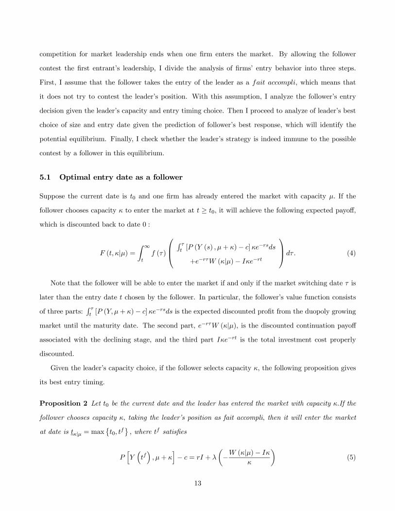
otherwise the leader will enjoy a period of monopoly before tμ|κ. Let t denote the leader’s entry date

and the leader’s payoff L (t, κ|μ) is

L (t, κ|μ) =

⎧⎪⎪⎪⎪⎪⎪⎪⎪⎪⎪⎪⎪⎪⎪⎪⎪⎪⎪⎨⎪⎪⎪⎪⎪⎪⎪⎪⎪⎪⎪⎪⎪⎪⎪⎪⎪⎪⎩

R tμ|κt f (τ)

⎡⎢⎣ R τt (P [Y (s) , κ]− c)κe−rsds

−e−rtIκ+ e−rτWmκ

⎤⎥⎦ dτ

+R∞tμ|κ

f (τ)

⎡⎢⎢⎢⎢⎣R tμ|κt (P [Y (s) , κ]− c)κe−rsds− e−rtIκ

+R τtμ|κ

(P [Y (s) , μ+ κ]− c)κe−rsds

+e−rτW (κ|μ)

⎤⎥⎥⎥⎥⎦ dτif t < tμ|κ

R∞t f (τ)

⎡⎢⎣ R τt (P [Y (s) , μ+ κ]− c)κe−rsds

−e−rtIκ+ e−rτW (κ|μ)

⎤⎥⎦ dτ if t ≥ tμ|κ

. (6)

16

( ( ( ), ) ) rs

tP Y s c e ds

τκ κ −−∫

mWκ

tκμτ

( )( ( , ) )t rs

tP Y s c e ds

κμ κ κ −−∫ ( )|W κ μ

tκμ τ

( )( ( , ) ) rs

tP Y s c e dsκ

μ

τκ μ κ −+ −∫

t

t

( )|W κ μ

tκμ τt

( )( ( , ) ) rs

tP Y s c e ds

τκ μ κ −+ −∫

O

1:Case If t t and tκ κμ μτ< <

2 :Case If t t and tκ κμ μτ< >

3:Case If t t and tκμ τ> >

Figure 2: Leader’s Payoff

Figure 2 illustrates the components of the leader’s payoff defined in Equation (6). In the first case,

the leader enters the market before the market maturity date τ is realized, and the market switches

before the follower’s optimal entry date, i.e., τ < tμ|κ. In this case, the leader will monopolize the market

until its exit and receive a payoff of two parts: a discounted profit stream,R τt (P [Y (s) , κ]− c)κe−rsds,

before the market switches, and a discounted monopoly continuation payoffWmκ in the declining stage22.

In the second case, if the market matures later than tμ|κ, the leader’s monopoly position ends at tμ|κ due

to the follower’s entry. So its payoff after tμ|κ consists of two part:R τtμ|κ

(P [Y (s) , κ+ μ]− c)κe−rsds,

monopoly profit before the market switches and a duopoly continuation payoff of W (κ|μ) . This case ischaracterized in the middle of Figure 2. Finally, case 3 considers the situation that the leader chooses

t ≥ tμ|κ. If so, the follower will enter the market immediately with capacity μ as long as its payoff is

nonnegative. In this case, the leader will be earning its duopoly profit immediately after its entry; i.e.,

its payoff as a leader equals the profit it would have earned had it entered as a follower with capacity

κ while its opponent enters earlier with capacity μ. Hence for t > tμ|κ, L (t, κ|μ) = F (t, κ|μ) .Proposition 3 implies that the follower’s optimal entry date will depend on the demand growth rate

α1. With the assumption αS < αL, there are three cases to consider. If α1 < αS, the follower always

chooses small capacity and if α1 > αL, the follower always builds a large plant regardless of the leader’s

capacity choice. The most interesting case is αS < α1 < αL, because if the leader chooses small capacity

22Wmκ is derived in Section 3.

17

S, the follower will select L,and if the leader chooses large capacity L the follower will choose S. As

a result, in the case of αS < α1 < αL, the leader might be able to preempt the follower with a large

capacity and thus force the follower to become a small competitor, which is the result usually predicted

in previous studies. However, this might not be the case if we account for the effect of option value on

firm’s strategic incentive. As a result, the discussion of firms’ equilibrium strategies are divided into

two subsections: we start with analyzing the equilibrium without leadership contest by presenting two

lemmas, after which, we introduce the possibility of leadership contest and demonstrate the effect of

option value on firms’ strategic preemptive incentives.

Equilibrium without Leadership contest

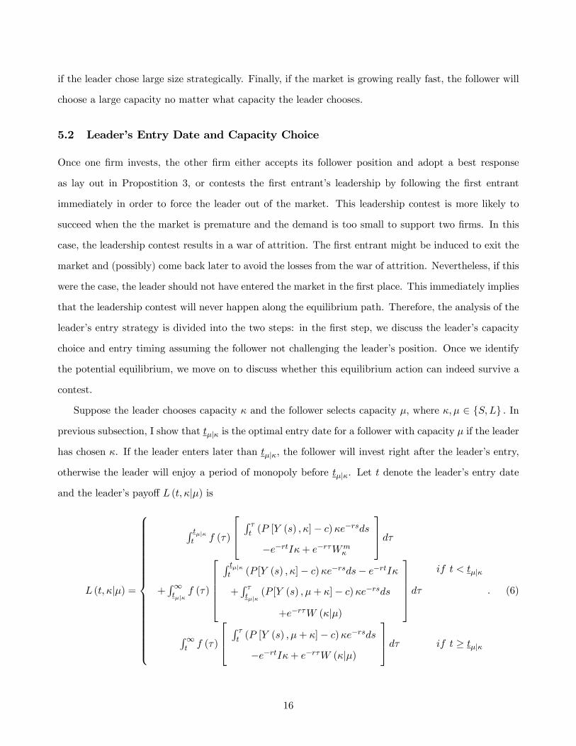
Because αS < α1 < αL, the leader and follower always choose different capacities. From Equation (6) ,

we know that the graph of the leader’s payoff function L (t, κ|μ) contains two concave curves linked attμ|κ. For t < tμ|κ, L (t, κ|μ) is first increasing in t until it reaches tmκ , the monopoly entry date for a firmwith capacity κ23. If t > tμ|κ, L (t, κ|μ) coincides with the payoff of a firm with capacity κ following a

leader with capacity μ. Figure 3 shows the leader’s and follower’s payoffs as a function of the leader’s

entry date. If the leader chooses L and the follower picks S, curve CEFGL maps the payoff function for

the large leader, L (t, L|S) . Note that this curve contains two parts, the first part (CEF ) is the payoffwhen the large leader enters before the follower’s optimal entry date tS|L, which reaches its maximum

at tmL , the monopoly entry date for a large firm. The second part (FGL) is the leader’s payoff if it enters

later than tS|L, which is less because its competitor will enter immediately after the leader’s entry. In

this case, the leader will not earn monopoly profit but will earn duopoly payoff after date tS|L, which

is overlapped with the payoff of a follower with capacity L after a leader with capacity S. The second

part of the leader L’s payoff is maximized at tL|S , which is greater than tS|L as shown in Corollary 2,

so the leader L’s payoff has a kink at F. Similarly, curve BDJK is the payoff for a leader with capacity

S when its follower selects capacity L.

23L (t, κ|μ) can be rewritten as L (t, κ|μ) = L (t, κ|0) − A (κ|μ) ,where L (t, κ|0) =R∞t

f (τ)¡R τ

t(y0e

α1sD (κ)− c)κe−rsds− e−rtIκ+ e−rτWmκ

¢dτ is the expected monopoly profit for a firm

with capacity κ to enter at date t, which is concave over t and maximized at tmκ , and A (κ|μ) =R∞tμ|κ

f (τ)

à R τtμ|κ

y0eα1s (D (κ)−D (μ+ κ))κe−rsds

+e−rτ (Wmκ −W (κ|μ))

!dτ is independent of the leader’s entry date t. The term

A (κ|μ) can be viewed as the negative impact on the leader caused by the presence of a follower. This term is decreasingin tμ|κ, i.e., the earlier the follower enters the market, the smaller the leader’s payoff will be. Therefore, when choosingits plant size, the leader has incentive to delay the entry of the follower as much as possible.

18

On the other hand, if the follower does not contest the leadership, it will not enter the market until

its optimal entry date as a follower. In particular, a follower with capacity L when following a leader

with capacity S will wait until tL|S , thus its payoff F (t, L|S) as a function of leader’s entry date t is aconstant before tL|S, which is shown as the horizontal line Y G in Figure 3. After date tL|S, the follower’s

payoff starts decreasing which is denoted by curve FL. So the curve Y GL is the large follower0s payoff.

Similarly, curve AHK depicts the small follower0s payoff.

V

t|L St|S Lt |L St

( ), |L t S L

( ), |L t L S

|S LtmSt

mLt

*t't

( ), |F t L S

( ), |F t S L

A

B C

D

F

G

HJ

K

L

X

Y

E

Figure 3: Leader and Follower’s payoff functions

Figure 3 illustrates the leader and follower’s payoff functions when they are of different capacities.

The following lemma gives the sufficient conditions for a unique intersection between two leader’s payoff

function to the left of tmL , which is point X in Figure 3.

Lemma 4 If L (0, S|L) > L (0, L|S) and L (tmS , S|L) < L (tmL , L|S) , there exists a unique t∗ < tmL such

that L (t∗, S|L) = L (t∗, L|S) .

This paper asks the question whether the first entrant can credibly preempt its follower with a large

capacity. L (tmκ , κ|μ) is the maximum payoff for a firm with capacity κ if it enter at its optimal entry

date tmκ . L (tmS , S|L) < L (tmL , L|S) gives the leader incentive to preempt the follower with large capacity,

which is a necessary condition when comparing with previous papers on Stackelberg leadership, because

in previous papers, the leader usually chooses a large capacity and receives more payoff than its follower.

As shown in Figure 3, if the leader is indeed exogenously chosen, it will choose large capacity as long as

19

L (tmS , S|L) < L (tmL , L|S). In order to compare our result to previous studies, I maintain the assumptionthat L (tmS , S|L) < L (tmL , L|S) , which implies that large capacity preemption is at least feasible and wecan focus on its credibility.24In addition, I assume that F

³tL|S, L|S

´> F

³tS|L, S|L

´, which implies

that the follower prefers to be preempted by a smaller firm rather than a larger firm because it can take

advantage of a faster-growing market by choosing larger capacity without too much concern about the

adverse option value effect. As a result, if the leader successfully installs a large capacity and commits

to staying in the market, the follower will suffer as a Stackelberg follower with less payoff.

Let LX denote the leader’s payoff at X. Because X is the intersection of two leader’s payoff functions

at date t∗,we must have LX = L (t∗, S|L) = L (t∗, L|S) . Since F³tL|S , L|S

´> F

³tS|L, S|L

´,there are

three cases to consider depending on the relationship between LX and two optimal payoffs of followers.

This is easily seen in Figure 3, horizontal line Y G corresponds to payoff level F³tL|S, L|S

´and line AH

corresponds to payoff level F³tS|L, S|L

´. Those two lines divided the vertical axis into three segments

and the intersection X may lie in any of the three segments. The following three lemmas studies those

two cases individually and discuss the preemption equilibrium with the assumption that the follower

takes the leader’s position as fait accompli.

Lemma 5 (Rent Equalization with a small leader)Suppose the follower takes the leader’s position as

fait accompli. If LX ≥ F³tL|S, L|S

´> F

³tS|L, S|L

´, the leader will enter at tS|L with capacity S and

the follower will enters at tL|S with capacity L, where tS|L satisfies L¡tS|L, S|L

¢= F

³tL|S , L|S

´.

This Lemma characterized a rent equalization equilibrium when firms are allow to choose both

capacity and entry timing. LX > F³tL|S , L|S

´implies that there exist two dates, tS|L and tL|S, such

that L¡tS|L, S|L

¢= L

¡tL|S, L|S

¢= F

³tL|S , L|S

´. In Figure 3, tS|L is the date at which the horizontal

line Y G crosses the smaller leader’s payoff function BDJK, which is the rent equalization date. That

is, if the smaller leader enters at this date, it earns the same expected payoff as the follower. However,

to reach the same payoff level, the leader with capacity L needs to wait until tL|S, which is later than

tS|L. Observe that tS|L < t∗, that is, large capacity preemption is not feasible, so the first entrant will

choose capacity S to enter the market at tS|L. This is due to two facts: first, the first entrant will not

enter the market before tS|L, because it can achieve higher payoff as a follower. On the other hand,

24 If this condition is violated, it means that the large capacity choice is actually an over capacity, which results in lowerpayoff even if the leadership is not contested. Therefore, even an exogenously determined leader would not choose largecapacity. See Wu(2005) for details.

20

it could not be an equilibrium for the leader to later than tS|L. To see why, suppose firm 1 is the

leader and enters at t > tS|L, firm 2 can always best respond by entering at t − ε to preempt firm 1,

which contradicts the fact that firm 1 is the leader. As a result, the leader has to enter with capacity

S at tS|L. Since no leadership contest is allowed, the follower will wait until its optimal entry date tL|S

and enter the market with capacity L. Previous studies usually assume the first entrant can enter the

market immediately. Suppose firms cannot invest until date t∗. The following lemma shows that there

is a symmetric subgame perfect equilibrium with first entrant preempting the second entrant with large

capacity and achieves higher expected payoff.

Lemma 6 If F³tL|S , L|S

´> LX > F

³tS|L, S|L

´and the market is not open until t∗, the leader enters

immediately at t∗ with capacity L and the follower will enter at tS|L with capacity S, where t∗ satisfies

L (t∗, S|L) = L (t∗, L|S) = LX .

For t < t∗, large capacity preemption is not feasible because the leader is better off by choose a

small capacity plant. Suppose the game starts at t∗, Lemma 6 proves that in equilibrium both firm

will try to preempt its competitor with a large capacity if no market contest will happen. This result

extends Maggi (1996) to a continuous-time setting: if immediate investment is possible, the leader will

try to invest in larger capacity, which trades off flexibility with the advantage of earlier commitment.25

This result relies on the assumption that the game begins at t∗. If the firm is allowed to move before t∗,

there is no pure strategy subgame perfect equilibrium with the leader enters as a large firm. Observe

that if firm 1’s strategy is to wait until t∗ to enter as a large firm. If firm 2 adopts the same strategy,

each firm has equal probability of entering as a large leader. So the expected payoff for firm 2 is

12L (t

∗, L|S) + 12F (t, S|L). However, firm 2 can improve its payoff by investing at t − ε with a smaller

capacity, which guarantees its winning of the leadership contest with a payoff slightly below L (t∗, L|S)but strictly greater than 1

2L (t∗, L|S) + 1

2F (t, S|L). On the other hand, the leader enters as a smallfirm is not an symmetric pure strategy equilibrium, because the other firm will choose not to enter the

market until t(L|S) so it can earn higher payoff as a large firm. The following lemma shows that thereexists a subgame perfect ε−equilibrium with the leader enters as a smaller firm first. A subgame perfectε−equilibrium is a strategy profile defined from a specific date t onwards when no player can deviate to

25Maggi (1996) considered a two stage setting with leader acts at the first stage but the market is not open until secondstage.

21

V

t|L St|S Lt|L St

( ), |L t S L

( ), |L t L S

|S LtmSt

mLt

( ), |F t L S

( ), |F t S L

cLtt*B

D

J

KC

E

F

G

L

M

X

Y

AH

Figure 4: Small Leader Large Follower

any other strategy and gain more than ε. If ε = 0, then this is a subgame perfect equilibrium.26

Lemma 7 If F³tL|S , L|S

´> LX > F

³tS|L, S|L

´, there is a subgame perfect ε−equilibrium with the

leader enters with capacity S and the followers enters with capacity L.

The case of F³tL|S, L|S

´> LX > F

³tS|L, S|L

´is shown in Figure 4. The difference between

Figure 4 and Figure 3 is that Y G crosses CE at a date later than t∗ because LX < F³tL|S , L|S

´. In

this case, in an asymmetric equilibrium, the leader enters with capacity S at a date slightly earlier than

t∗ and the follower wait until tL|S . In fact, as shown in Figure 4, if the leader enters later than t∗, it

is always better off by choosing large capacity rather than small capacity. However, competition for

market leadership will force the first entrant to enter earlier than t∗ with a smaller capacity.

Finally, if F³tL|S , L|S

´> F

³tS|L, S|L

´≥ LX , the following lemma shows another rent equalization

equilibrium with the leader entering as a large firm and the follower being the smaller firm. In this case,

both firms are earning the same payoff and the large capacity preemption is credible if the follower is

not allowed to contest its leadership.

Lemma 8 (Rent equalization with a large leader)Suppose the follower takes the leader’s position as

fait accompli. If F³tL|S, L|S

´> F

³tS|L, S|L

´≥ LX , the leader will enter at tL|S with capacity L and

the follower will enters at tS|L with capacity S, where tL|S satisfies L¡tL|S , L|S

¢= F

³tS|L, S|L

´.

26Please see Laraki et.al. (2003) for more discussions on this concept applied to continuous-time games of timing.

22

V

t|L St|L St

( ), |L t S L

( ), |L t L S

|S LtmSt m

Lt

( ), |F t L S

( ), |F t S L

t*B

D

J

KC

E

F

G

L

M

X

Y

A

H

|S Lt

Figure 5: Rent equalisation with large leader

Contestability Condition

In previous subsection, I assume that the follower will not contest the first entrant’s leadership. Re-

moving this assumption opens the possibility for the follower to challenge the first entrant’s leadership.

In particular, the follower, after seeing its competitor entering the market, has two options: it can wait

until its optimal entry date as a follower or it can enter earlier and trigger a war of attrition in the

growing market. Of course, it would not start a war unless it could force the leader out of the market,

otherwise it would have entered at a suboptimal date. An immediate implication is that choosing the

same capacity to contest the leadership will not succeed, because both firms will earn the same payoff

and the leader does not have a dominant strategy to exit the market. Consequently, a firm will contest

the other firm’s leadership if and only if, by choosing a different capacity, it can replace the leader as a

monopoly by driving it out of the market.

Therefore, we simply need to discuss the leadership contest between a small firm and a large firm.

Once war of attrition is triggered, if neither firm is earning positive payoff, both firms might want to

exit the market. As this is a war of attrition happens along the growing market, the winner depends on

which firm has a shorter exit region. In particular, the following proposition shows that if the war of

attrition is started at t0, each firm has a continuous exit region in the form of [t0, tcκ] where κ ∈ {S,L} ,and tcκ is the last date that a firm with capacity κ wants to exit the market as long as the market

continues to grow. The following proposition identifies the winner by comparing the last exit dates tcκ.

23

Proposition 4 If a war of attrition happens at t < tcL =1α1ln

c−λW (L|S)L

y0D(S+L)between a firm with capacity

S and the other firm with capacity L when the market is growing, the firm with capacity L will exit the

market immediately.

Because the market demand is growing, for a firm with capacity κ {∈ {S,L}} , tcκ is the last day thatit will consider exiting the market. Therefore, by comparing tcS and t

cL, we can identify the equilibrium in

this war of attrition subgame. In the proof, I show that tcκ =1α1ln

c−λW (κ|μ)κ

y0D(S+L), κ 6= μ. A quick comparison

of tcS and tcL reveals that the only difference is an item on the numerator, W (κ|μ)κ , which is the per

unit capacity marginal option value for a firm to delay its exit from the market. To see why, suppose

the market is growing at the moment. Observe that W (κ|μ) is also the continuation payoff for a firmwith capacity κ after market swtiches. By choosing to stay in the market in the war of attrition, the

firm can avoid losing W (κ|μ) when the market suddenly switches to decline, which, multiplied by theprobability of market switching λ, is exactly the expected potential losses avoided by choosing not to

exit the market, or in a word, it is the option value of delaying exit.

Corollary 1 shows that W (S|L)S > W (L|S)

L , which implies tcS < tcL. This is, a smaller firm has higher

option value and thus reduces its willingness to exit the market. As a result, its exit region is shorter

than that of the large firm. In turn, this implies that if the leader chooses capacity L and enters at

t < tcL, then the other firm can enter immediately with a smaller capacity and force the leader out of

the market, because once the war of attrition is triggered, the exit region of the follower is [t, tcS] ,which

is shorter than [t, tcL] ; hence in a subgame perfect equilibrium the firm with the larger capacity will

not be able to win the war of attrition because for the subgame beginning at t > tcS , the smaller firm

definitely will stay in the market while the large firm is still in its exit region.

Given this result, we can check the contestability condition in the two cases discussed in the previous

subsection. In particular, if tL|S < t∗ as shown in Figure 3, Lemma 5 proves that the smaller firm can

enter the market earlier if the follower takes the leader as fait accompli. If the follower is allowed to

contest the first mover’s lead, the smaller leader can still survive because its advantage in winning the

war of attrition further strengthens its credibility to stay in the market.

However, this is not the case when t∗ < tL|S . First, a firm choosing smaller capacity will not enter

the market until tS|L which guarantees it at least as much payoff as the follower. However, if the firm

chooses to be large, its leader’s payoff will reach this level at tL|S which is earlier than tS|L. In fact, the

24

leader is better off by choosing large capacity if it wants to enter later than t∗. The question is whether

it can credibly choose large capacity to preempt the follower. The following proposition summarizes

those two cases and gives a set of sufficient conditions under which the leader holds its entry until tS|L,

at which time it starts operation in a small capacity.

Proposition 5 Given Assumptions 1-5 and assuming αS < α1 < αL, and L (tmL , L|S) > L (tmS , S|L) >F³tL|S, L|S

´> F

³tS|L, S|L

´, there is a unique subgame perfect equilibrium in which the leader enters

at tS|L with smaller capacity S while the follower enters at tL|S with larger capacity, if the following

conditions are satisfied:D (S)

D (S + L)≥ c+ rI + φ (S|L)

c(7)

where φ (S|L) = −λ³W (S|L)

S − I´.

The condition αS < α1 < αL implies that the resulting duopoly market structure is asymmetric

with one small firm and one large firm. Condition (7) is a sufficient condition that guarantees that

a small firm will win the war of attrition in the growing stage, because D(S)D(S+L) ≥ c+rI+φ(S|L)

c implies

tmS ≤ tcL, which is a sufficient condition for tS|L < tcL since tS|L ≤ tmS . This condition implies that if the

larger firm entered earlier than tS|L, it would be forced out by a smaller firm. Hence a large firm should

not enter the market even with tL|S < tS|L. The proof of the proposition considers two cases. When

tL|S ≤ t∗, as shown in Figure 3, we have tS|L < tL|S , in which case it is intuitively evident that the

smaller firm can enter earlier credibly. In contrast, tL|S > t∗, as shown in Figure 4, a larger firm is able

to enter earlier by the rent equalization principle, but its action is not credible. Since tS|L < tcL, if the

first firm selects larger capacity to preempt the second firm, the second firm can enter at tS|L to force

the first one out of the market. In this sense the larger capacity preemption is simply not credible.

Note that condition (7) is a sufficient condition. Actually as long as tS|L < tcL, the smaller firm can

always wait until tS|L to enter the market, because no larger firm will be able to preempt its competitor,

otherwise it would be forced out by a smaller firm at tS|L.

Finally, we briefly discuss two other cases: one is when the market growth rate α1 < αS and the

other is α1 > αL. In both cases, the main economic forces that drive the result are those two analyzed in

the previous section: first, a higher option value causes a firm with large capacity to delay its investment

timing, which in turn reduces its incentive to preempt its competitor. Second, even if the first entrant

25

is able to enter the market with a large capacity, it might not want to build a large plant because it

may not survive the leadership contest if its follower jumps into the market with a small capacity. In

particular, if α1 < αS, the follower always enters at a smaller capacity no matter what capacity the

leader chooses. In this case, if the leader wants to choose large capacity, it must take into account the

disadvantage it faces when the market switches. Under some similar conditions in equilibrium both the

leader and follower will enter the market with small capacity.27 This will be the case when firms are

impatient given the uncertainty of the market, for example in the Wi-Fi market, some people claim that

the most important question faced by the potential entrants is not how large its size is, but how fast it

enters the market.28

If the market is growing very fast as α1 > αL, a noncontesting follower always chooses large capacity

to enter the market. Whether the leader chooses large capacity will completely depends on whether the

follower will be able to use small capacity to force the leader out of the market, because the follower will

only choose small capacity if she is able to start a war of attrition and gets higher payoff. Therefore, we

can apply a similar analysis and the discussion is omitted here since in equilibrium the leader will always

choose a capacity to prevent a follower from contesting its leadership. As a result, it never chooses a

capacity greater than its follower.

6 Discussions

6.1 Multiple Capacities

In the previous discussions, there are two essential assumptions: capacity choice is binary and the path

of market evolution is discontinuous at the date when market switches. The latter is justified because

in many cases the introduction of new product by a third party has a significant negative effect on

the demand for the old product. In fact, the main intuition of the paper does not rely on either of

these assumptions. As long as the number of capacity levels is finite, the numerical analysis will be

reduced to a comparison of two capacity levels. I relax both assumption by computing a numerical

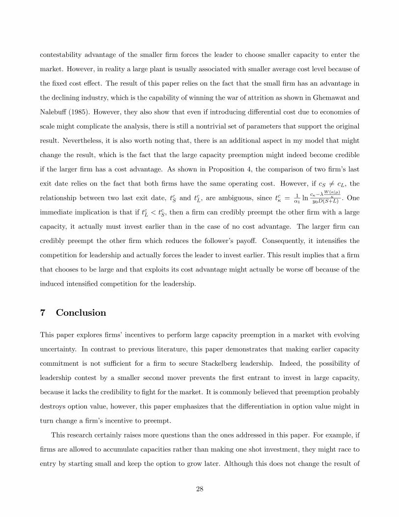
example with three capacities choices and continuous market evolution. Table 1 is list the results of

27The proofs of those results are available upon request. I omitted the details here since it only provides limited additionalinsights.28See "Cometa hot spots to get cold shoulder?", CNET news.com. July 21, 2003.

26

Table 1: Leader and follower’s equilibrium payoffs and capacity choices

Leader Followerα1 Capacity Payoff Capacity Payoff0.15 1.5 4.674 1.5 4.6740.16 1.5 6.495 1.5 6.4950.17 1.5 8.833 1.5 8.8330.18 1.8 9.944 1.5 9.9440.19 1.8 13.26 1.5 13.260.20e 1.5 18.20 1.8 20.940.21e 1.5 22.39 1.8 27.540.22 1.8 30.88 1.8 30.880.23 1.8 55.07 1.8 55.070.24 1.8 75.32 1.8 75.32

Source: Calculated by the author.

Parameters : y0= 0.2;λ = 0.2;α2= −0.3; r = 0.1; I = 50; c = 3.Firm Capacity Choices: Q = {1.5, 1.8, 2.1}e : ε− equilibrium;

numerical solution of a model with three capacities. The algorithm is very simple. First, we derive the

noncontesting follower’s optimal capacity choice given the leader’s different capacity choices. Second,

we investigate which rent equalization equilibrium is most preferred by the leader and check whether

it can sustain a potential contest from the follower. If not, we keep tracking other equilibria. Table 1

illustrates three types of equilibria: rent equalization with equal capacities, rent equalization with large

leader and asymmetric ε − equilibrium with smaller leader. A common pattern is that the leader is

not better off than the follower and some times earning less payoff than the follower. In particular, if

α1 = 0.20 or 0.21, if market opens right at the first date that the leader is indifferent from choosing

large or small capacity, that is, date t∗ in previous discussion, the leader will be able to choose large

capacity and earns higher payoff, as proved in previous section. However, it is not an equilibrium for

both firm to wait until this day to compete for the Stackelberg leadership with a large capacity.

6.2 Cost Advantage

In my model, firms have the same unit cost regardless of its plant size. Proposition 4 shows that the

smaller firm always has an advantage in the war of attrition. Especially if the market is growing, the

27

contestability advantage of the smaller firm forces the leader to choose smaller capacity to enter the

market. However, in reality a large plant is usually associated with smaller average cost level because of

the fixed cost effect. The result of this paper relies on the fact that the small firm has an advantage in

the declining industry, which is the capability of winning the war of attrition as shown in Ghemawat and

Nalebuff (1985). However, they also show that even if introducing differential cost due to economies of

scale might complicate the analysis, there is still a nontrivial set of parameters that support the original

result. Nevertheless, it is also worth noting that, there is an additional aspect in my model that might

change the result, which is the fact that the large capacity preemption might indeed become credible

if the larger firm has a cost advantage. As shown in Proposition 4, the comparison of two firm’s last

exit date relies on the fact that both firms have the same operating cost. However, if cS 6= cL, the

relationship between two last exit date, tcS and tcL, are ambiguous, since tcκ =1α1ln

cκ−λW (κ|μ)κ

y0D(S+L). One

immediate implication is that if tcL < tcS , then a firm can credibly preempt the other firm with a large

capacity, it actually must invest earlier than in the case of no cost advantage. The larger firm can

credibly preempt the other firm which reduces the follower’s payoff. Consequently, it intensifies the

competition for leadership and actually forces the leader to invest earlier. This result implies that a firm

that chooses to be large and that exploits its cost advantage might actually be worse off because of the

induced intensified competition for the leadership.

7 Conclusion

This paper explores firms’ incentives to perform large capacity preemption in a market with evolving

uncertainty. In contrast to previous literature, this paper demonstrates that making earlier capacity

commitment is not sufficient for a firm to secure Stackelberg leadership. Indeed, the possibility of

leadership contest by a smaller second mover prevents the first entrant to invest in large capacity,

because it lacks the credibility to fight for the market. It is commonly believed that preemption probably

destroys option value, however, this paper emphasizes that the differentiation in option value might in

turn change a firm’s incentive to preempt.

This research certainly raises more questions than the ones addressed in this paper. For example, if

firms are allowed to accumulate capacities rather than making one shot investment, they might race to

entry by starting small and keep the option to grow later. Although this does not change the result of

28

this paper, it does warrant further studies. Most recent studies on industry dynamics have been focused

on the asymmetries generated by firm specific idiosyncrasies as pioneered by Ericson and Pakes (1995) ,

while literature has been pretty silent on the evolution of industry structure due to firms’ strategic

interactions under uncertainty, which is of course a topic for future research.

8 Appendix

Proof of Lemma 1

Proof. (i) By Assumption 4, y = cD(2S) . Substitute it into Equation (2) and obtains firm’s monopoly

exit date, txκ =1α2ln D(2S)

D(κ) , which is counting from the market switching date τ . As a result, its exit

date with respect to date 0 is tx (τ , κ) = τ + 1α2ln D(2S)

D(κ) . In particular, D (S) > D (L) implies txS > txL

and thus tx (τ , S) > tx (τ , L) for all τ .

(ii) Note that Wmκκ =

R txκ0 (yeα2sD (κ)− c) e−rsds. This result follows immediately from the facts

that D (S) > D (L) and txS > txL.

Proof of Lemma 2

Proof. Consider a firm with capacity κ, κ ∈ {S,L} , its expected payoff when entering at date t is:

M (t, κ) =

Z ∞

tf (τ)

µZ τ

t(y0e

α1sD (κ)− c)κe−rsds+ e−rτWmκ − Iκe−rt

¶dτ

Hence∂M (t, κ)

∂t= e−(λ+r)t

¡−y0eα1tD (κ)κ+ cκ+ (λ+ r) Iκ− λW 0κ

¢= 0

Therefore let tmκ denote the solution of the above first order conditions, we have

P (Y (tmκ ) , κ)− c = rI + λ

µ−W

mκ − Iκ

κ

¶

where P (Y (tmκ ) , κ) = y0eα1tmκ D (κ) , and it is routine to check that the second order condition is

satisfied at tmκ :

tmκ =1

α1ln

c+ (λ+ r) I − λWmκκ

y0D (κ)

29

Since WmSS >

WmLL and D (S) > D (L) , we must have

tmS < tmL .

Proof of Proposition 1

Proof. Let t be the current date, and suppose the market switches at τ . Define t0 = t − τ to be

the current date counting from the switching date τ . Once the decline stage begins, if two firms are of

different sizes, then we know the market price is

p (y, S + L) = yD (S + L) < yD (2S) = c

This implies that if both firms stay in the market, they will be earning negative profit. Also note

that no firm will stay longer than its monopoly exit date txκ, κ = S,L. Hence we only need to consider

the date t0 < txS .

If txS > t0 > txL, the larger firm will exit the market immediately because even if the smaller firm

leaves the market in the next instant and the larger firm becomes a monopoly, it will still exit the

market because it has already passed its monopoly exit date. Realizing that the dominant strategy for

the larger firm is to leave, the smaller firm will stay in the market.

Consider the case of txL ≥ t0 ≥ 0. If t0 = txL, the larger firm will exit the market for sure and the

smaller firm will stay. Consider t0 = txL − ε, by staying in the market, the smaller firm will incur a loss

until date txL when the larger firm leaves the market. Hence the smaller firm’s profit is

Z txL

txL−ε(yeα2sD (S + L)− c)Se−rsds+

Z txS

txL

(yeα2sD (S)− c)Se−rsds > 0

for ε sufficiently small. Therefore, the smaller firm will stay in the market for sure. In this case, the

larger firm will have to leave the market at t0 = txL− ε. By the same reasoning, the larger firm will leave

the market at each date t0 ≥ 0. Hence we have proved part (i) .(ii) In this case two firms are of the same size. By Assumption 2, firm i0s size is decreased by

δi, i = 1, 2. With probability 12 , δ1 > δ2. In this case, ex post firm 1 will become smaller than the other

30

firm. By the same reasoning of part (i) , firm 2 will have to exit the market earlier than firm 1, while

the latter can stay until its monopoly exit date. As a result, if δ → 0, firm 2 will exit immediately after

market switches.

Proof of Proposition 2

Proof. Differentiating (4) with respect to t, we will have

∂F (t, κ|μ)∂t

= −f (t) ¡e−rtW (κ|μ)− Iκe−rt¢

+

Z ∞

tf (τ)

¡¡−y0eα1tD (μ+ κ)− c¢e−rtκ+ rIκe−rt

¢dτ = 0

which can be simplified as

y0eα1tD (μ+ κ)− c = rI + λ

µ−W (κ|μ)− Iκ

κ

¶

Thus29

tf =1

α1ln

c+ rI + λ³−W (κ|μ)−Iκ

κ

´y0D (μ+ κ)

In particular, t0 > tf , then the firm will enter immediately since its payoff is decreasing.

Proof of Lemma 3

Proof. Note that

αL − αS

= (λ+ r)

³ln D(L+S)

D(2L) − ln ηL´¡ln L

S − ln ηS¢− ³ln D(2S)

D(S+L) − ln ηS´¡ln L

S − ln ηL¢¡

ln LS − ln ηL

¢ ¡ln L

S − ln ηS¢

=(λ+ r)¡

ln LS − ln ηL

¢ ¡ln L

S − ln ηS¢⎡⎢⎢⎢⎢⎣ln L

S

³ln D(L+S)

D(2L) − ln D(2S)D(S+L)

´− ln ηS

³ln D(L+S)

D(2L) − ln LS

´− ln ηL

³ln L

S − ln D(2S)D(S+L)

´⎤⎥⎥⎥⎥⎦

29 It is easy to check the second-order condition is satisfied.

31

So αL > αS if and only if

ln LS

³ln D(L+S)

D(2L) − ln D(2S)D(S+L)

´− ln ηS

³ln D(L+S)

D(2L) − ln LS

´− ln ηL

³ln L

S − ln D(2S)D(S+L)

´ > 0. In particular, if D (Q) = a− bQ, it is

routine to check that 2L+ S > ab > L+ 2S is sufficient.

Proof of Proposition 3

Proof. Note that

F (t, κ|μ) =Z ∞

tf (τ)

µZ τ

t(y0e

α1sD (μ+ κ)− c)κe−rsds+ e−rτW (κ|μ)− Iκe−rt¶dτ

From the first order condition, we know that y0eα1tκ|μD (μ+ κ)κ = cκ+ (λ+ r) Iκ− λW (κ|μ) .Hence

we must have

Fμκ

³tκ|μ

´= e−(λ+r)tκ|μ (cκ+ (λ+ r) Iκ− λW (κ|μ))

µα1

(λ+ r − α1) (λ+ r)

¶

HenceFμS

³tS|μ

´FμL

³tL|μ

´ = e−(λ+r)

³tS|μ−tL|μ

´c+ (λ+ r) I − λW (S|μ)

S

c+ (λ+ r) I − λW (L|μ)L

S

L

Define ημ =c+(λ+r)I−λW (S|μ)

S

c+(λ+r)I−λW (L|μ)L

≤ 1. Note that tS|μ − tL|μ =1α1lnhD(μ+L)D(μ+S)η

μi.Hence

FμS

³tS|μ

´FμL

³tL|μ

´ = ∙D (μ+ L)

D (μ+ S)ημ¸−λ+r

α1

ημS

L

Therefore, if α1 < αμ =(λ+r)[lnD(μ+S)−lnD(μ+L)−ln ημ]

lnL−lnS−ln ημ , FμS

³tS|μ

´> Fμ

L

³tL|μ

´. The results of the

proposition then follow naturally.

32

Proof of Lemma 4

Proof. Since L (0, S|L) > L (0, L|S) , L (tmS , S|L) < L (tmL , L|S) implies that there exists a t∗ such thatL (t∗, S|L) = L (t∗, L|S) . Also note that

∂L(t,S|L)S

∂t− ∂L(t,L|S)

L

∂t= e−(λ+r)t

µ−λ

µWm

S

S− Wm

L

L

¶− y0e

α1t (D (S)−D (L))

¶< 0

Hence, we must have ∂L(t,S|L)∂t =

∂ L(t,S|L)S∂t S <

∂ L(t,S|L)S∂t L <

∂ L(t,L|S)L∂t L = ∂L(t,L|S)

∂t . That is, for all

tmL > t > t∗, L (t, L|S) > L (t, S|L) and for all t < t∗, L (t, L|S) < L (t, S|L) , which proves theuniqueness of t∗.

Proof of Lemma 5

Proof. First, LX > F³tL|S , L|S

´implies that there exists two dates tS|L < t∗ and tL|S < t∗ such

that L¡tS|L, S|L

¢= L

¡tL|S, L|S

¢= F

³tL|S , L|S

´. As shown in Figure 3, tS|L and tL|S are two dates

at which Y G crosses two payoff functions L (t, S|L) and L (t, L|S) , respectively. We are considering asymmetric equilibrium. Without loss of generality, suppose firm 1 is the leader. As shown in Figure 3,

firm 1 has no incentive to enter as a larger firm before date t∗. If firm 1 enters at tS|L with capacity

S, firm 2 will best respond by entering at tL|S with capacity L and earning the same payoff. If firm

1 chooses to enter at t > tS|L, firm 2 will enter at t − ε to secure its leadership,which contradicts the

assumption that firm 1 is the leader. On the other hand, if firm 1 enters at t < tS|L, the follower has no

incentive to compete for the leadership at t since by waiting until date tL|S it can earn higher expected

payoff by investing in larger capacity. But given this, firm 1 can actually delay its entry and earn higher

payoff. As a result, the unique Markov perfect equilibrium is the leader enters at tS|L with capacity S

and the follower enters at tL|S with capacity L.

8.1 Proof of Lemma 6

Proof. We first show that the strategy described in this lemma is indeed an equilibrium. Without loss

of generality, assume that firm 1 is the leader. If firm 1 succeeds in entering at t∗ with capacity L, firm

2’s best response is to choose small capacity and enter at tS|L as shown in Proposition 3. However, if

firm 1 chooses to enter later than t > t∗, firm 2’s best response is to enter earlier with capacity L at

33

t− ε, since it will guarantee its leadership and a higher expected payoff than if it tries to compete for

leadership at t.

8.2 Proof of Lemma 7

Proof. Because L (t, S|L) is continuous and strictly greater than L (t, L|S) for t < t∗, there exists t

such that for t ∈ [t, t∗), LX −L (t, S|L) < ε. Define a strategy profile as follows: firm 1 enters at t with

capacity S if no firm has entered before t, otherwise enters as L at t∗ if no firm has enters between t and

t∗, otherwise enter at t (S|L) if firm 2 has built a plant of capacity L otherwise enter at t(L|S) if firm 2

has invested with capacity S. Firm 1 enters at t∗ with capacity L if no firm has entered, otherwise, enter

at t (S|L) if firm 1 has built a plant of capacity L otherwise enter at t(L|S) if firm 1 has invested with

capacity S. I claim this is a subgame perfect ε−equilibrium. To see why, given firm 2’s strategy, firm 1

had better enter as a small firm before t∗ to guarantee itself a payoff slightly below LX , in particular,

firm 1 cannot deviate its entry time later than t∗ because firm 2 would have entered with capacity L

at t∗. On the other hand, firm 1 will not profit more than ε by deviating to any date between t and t∗.

On the other hand, give firm 1’s strategy, firm 2 has no incentive to deviate since its payoff is strictly

higher.

8.3 Proof of Lemma 8

Proof. Define the firm 1’s strategy as follows: enter at tL|S with capacity L if no firm has enter the

market, otherwise if firm 2 has built a plant with capacity S, entering at tL|S with capacity L, or if

firm 2 has built a plant with capacity L, enter at tS|L with capacity S. Given firm 1’s strategy, I claim

that firm 2’s best response is to adopt the same strategy. To see why, observe that if F³tL|S , L|S

´>

F³tS|L, S|L

´≥ LX , as shown in Figure (??), entering earlier than tL|S is not optimal since it is better

off even it was preempted by firm 1 with large capacity. Entering later than tL|S will result being

preempted by firm 1. As a result, the best response is to enter as a large firm at the tL|S . In this case,

the leader and follower earns the same payoff.

34

Proof of Proposition 4

Proof. Suppose a firm chooses capacity κ and its competitor chooses μ where κ 6= μ and both κ and μ

∈ {S,L} . Firm κ needs to choose an exit date tκ when the market is growing to maximize its expected

value:

V xκ (tκ) = max

tκ>t

Z tκ

tf(τ)

µZ τ

t(y0e

αsD (S + L)− c)κe−rsds+ e−rτW (κ|μ)¶dτ (8)

+

Z ∞

tκ

f (τ)

µZ tκ

t(y0e

αsD (S + L)− c)κe−rsds+V cκ

Pr (τ > tκ)

¶dτ

The first part of (8) is the expected payoff when the market switches before the exit date chosen by firm

κ for the growing industry while the second part is the expected payoff when firm κ exits the market at

tκ. Note that, once Firm κ exit the market, it will achieve a continuation payoff V cκ which is independent

of its exit date. Let tcκ be the unique solution of the following equation,

∂V xκ (tκ)

∂tκ= f (tκ)

µZ tκ

t(y0e

α1sD (S + L)− c)κe−rsds+ e−rtκW (κ|μ)¶

−f (tκ)µZ tκ

t(y0e

α1sD (S + L)− c)κe−rsds¶

+

Z ∞

tκ

f (tκ)¡¡y0e

α1tκD (S + L)− c¢κe−rtκ

¢= e−(λ+r)tκ+λt

¡λW (κ|μ) + ¡y0eα1tκD (S + L)− c

¢κ¢

= 0

That is

tcκ =1

α1ln

c− λW (κ|μ)κ

y0D (S + L)

Since S < L and W (S|L) > 0 =W (L|S) ,

c− λW (S|L)

S< c− λ

W (L|S)L

we must have

tcS < tcL

which means that the smaller firm has a shorter exit region than the larger firm. Hence the smaller firm

35

can win the war of attrition in the growing industry, because once the date reaches tcS , if the smaller firm

stays in the market, then the larger firm will exit immediately. By working backward, we can prove the

result. This proves the result that the larger firm can not contest the smaller firm’s monopoly position.

Proof of Proposition 5

Proof. Since tcL =1α1ln c

y0D(S+L)and tmS = 1

α1ln

c+rI−λµWmSS−I¶

y0D(S), D(S)D(S+L) ≥

c+(λ+r)I−λWmSS

c implies

tcL − tmS ≥ 0.Also tL|S < t∗ implies tL|S < tS|L. Suppose tL|S ≥ tS|L. then we have

F³tL|S , L|S

´= L

¡tL|S , L|S

¢> L

¡tS|L, L|S

¢> L

¡tS|L, S|L

¢= F

³tL|S, L|S

´,

which is a contradiction. Note that tS|L < tmS implies tL|S < tcL. Therefore, the leader will not enter

the market with a large capacity because it will be forced out by a follower with a smaller capacity.

Given that the follower enters at tL|S with a payoff of F³tL|S, L|S

´, the leader will not enter earlier

than tS|L since for t < tS|L, L (t, L|S) < L (t, S|L) < F³tL|S, L|S

´. On the other hand, if the leader

delays entry at tS|L, the other firm will enter the market immediately. However, if the leader enters at

tS|L with a smaller capacity, the other firm will not preempt the leader by entering earlier because its

payoff is smaller by preempting the leader. It cannot force the leader out of the market by investing in

larger capacity. Hence, the follower’s best response to the leader’s entry at tS|L is to wait until tL|S and

enter with a large capacity.

Proof of Lemma ??

Proof. First we will show that simultaneous entry is not an equilibrium. Suppose the two firms choose

to enter simultaneously with the same capacity μ. In this case, they will choose to enter at date tμ|μ.

However, since L¡tmμ , μ|μ

¢> F

³tμ|μ, μ|μ

´, it is always better for one firm to deviate and enter earlier

at tmμ and achieve better payoff. There is no equilibrium in simultaneous entry. Hence, in a pure strategy

equilibrium, we must have one firm chooses to be a leader and the other to be a follower.

Suppose firm 1 chooses l and firm 2 chooses f in the precommitment stage. Since L (tmL , L|S) >L (tmS , S|S) and given that firm 2 chooses S, the best response for firm 1 is to chooses large capacity L

36

to enter at date tmL . On the other hand, α1 < αL implies F³tS|L, S|L

´> F

³tL|L, L|L

´. Provided that

firm 1 will commit to its investment and there is no exit allowed, firm 2’s best response is to choose S

and enter at tS|L.

References

[1] Anderson,S, J, Goeree and C. Holt (1998) , "The War of Attrition with Noisy Players". Advances

in Applied Micro-Economics, Volume 7, M. R. Baye, ed., Greenwich, Conn.: JAI Press, 1998,

15-29.

[2] Bernanke, B. S.(1983), “Irreversibility, Uncertainty and Cyclical Investment”, Quarterly Journal

of Economics, 98, 85-106.

[3] Dixit, A. (1980) , "The Role of Investment in Entry Deterrence". Economic Journal, Vol. 90, No.

357, 95-106

[4] Dixit, Avinash K., and Robert S. Pindyck (1994), Investment under Uncertainty. New Jersey:

Princeton University Press.

[5] Duffie, D (2001) , Dynamic Asset Pricing Theory. New Jersey: Princeton University Press.

[6] Dutta, P., S. Lach and A. Rustichini (1995) , "Better Late than Early: Vertical Differentiation

in the Adoption of a New Technology". Journal of Economics & Management Strategy, Vol.4,

No.4, 563-589

[7] Fudenberg, D. and J. Tirole (1985) , "Preemption and Rent Equalization in the Adoption of New

Technology". Review of Economic Studies, 52(3): 383-401

[8] Fudenberg,D. and J. Tirole (1986) , "A Theory of Exit in Duopoly." Econometrica, Vol. 54. 943-960.

[9] Gal-Or, E. (1985). First and second mover advantages. International Economic Review, 26, 649-653.

[10] Ghemawat, P. and B. Nalebuff (1985) , "Exit", Rand Journal of Economics, Vol. 16, No.2, 184-194.

[11] Grenadier, S. R. (1996) , "The strategic exercise of options: Development cascades and overbuilding

in real estate markets", Journal of Finance, Vol. 51(5), 1653-1679.

[12] Hamilton, J. and S. Slutzky (1990) , "Endogenous Timing in Duopoly Games: Stackelberg or

Cournot Equilibria", Games and Economic Behavior 2, 29-46.

37

[13] Hirokawa, M and D. Sasaki (2001) , "Endogenously asynchronous entries into an uncertain indus-

try", Journal of Economic Management and Strategy, Vol 10(3) , 435-461

[14] Laraki, R. E. Solan and N Vieille (2003) ,"Continuous-time Games of Timing", mimeo, HEC.

[15] Londregan, J. (1990) , "Entry and Exit Over the Industry Life-Cycle", Rand Journal of Economics,

Vol 23(3), 446-458

[16] Maggi, G. 1996, "Endogenous leadership in a new market", Rand Journal of Economics, vol. 27,

No. 4, pp. 641-659.

[17] Murto,P.(2004) ,"Exit in duopoly under uncertainty", Rand Journal of Economics, Vol 35(1), 111-

127.

[18] Rochet, J.C. and J. Tirole(2003), "Platform Competition in Two-Sided Markets," Journal of the

European Economic Association, 1(4): 990-1029.

[19] Ruiz-Aliseda, F. (2003) , "Strategic Commitment versus Flexibility in a Duopoly with Entry and

Exit". CMS-EMS Discussion Paper #1379, Northwestern University

[20] Ruiz-Aliseda, F and J. Wu (2004) , "Irreversible Investment in a Stochastically Cyclical Market".

mimeo. Northwestern University

[21] Sadanand, A. and V. Sadanand (1996), "Firm scale and the endogenous timing of entry: A choice

between commitment and flexibility", Journal of Economic Theory, vol. 70, no. 2, 516-530.

[22] Simon, L and M. Stinchcombe (1989) , "Extensive Form Games in Continuous Time: Pure Strate-

gies". Econometrica, Vol. 57, No. 5, 1171-1214

[23] Tirole, J. (1988) , The Theory of Industrial Organization, Cambridge, MA: M.I.T. Press.

[24] van Damme and Hurkens (1999) , "Endogenous Stackelberg Leadership", Games and Economic

Behavior, 28, 105-129

[25] von Stackelberg, H (1934) , Marktform und Gleichgewicht. Springer, Vienna.

[26] Weeds, H. (2002) , "Strategic delay in a real options model of R&D competition", Review of Eco-

nomic Studies, Vol. 69(3) , 729-747.

[27] Wells, J.R. "Note on the Aluminum Industry, 1983." Harvard Business School Case Study, #9-

386-092 and 9-386-093, 1985.

38

[28] Whinston, M. (1988) , "Exit with Multiplant Firms", Rand Journal of Economics, Vol 19(4) , 568-

588.

39