Creating Probabilistic Databases from IE Models Olga Mykytiuk, 21 July 2011 M.Theobald.

Creating Probabilistic Databases from IE Models

Olga Mykytiuk, 21 July 2011M.Theobald

2

Outline

Motivation for probabilistic databases Model for automatic extraction Different representation

One-row model Multi-row model

Approximation methods One-row model approximation Enumeration-based approach Structural approach Merging

Evaluation

3

Motivation

Ambiguity: Is Smith single or married? What is the marital status of Brown? What is Smith's social security number: 185 or 785? What is Brown's social security number: 185 or 186?

4

Motivation

Probabilistic database: Here: 2 × 4 × 2 × 2 = 32 possible

readings → can easily store all of them 200M people, 50 questions, 1 in 10000

ambiguous (2 options)→ possible readings

5

Sources of uncertinity

Certain Data Uncertain Data

The temperature is25.634589 C. Sensor reported 25 +/- 1 C.

Bob works for Yahoo. Bob works for Yahoo orMicrosoft.

UDS is located inSaarbrücken.

UDS is located inSaarland.

Mary sighted a crow. Mary sighted either a crow(80%) or a raven(20%).

It will rain in Saarbrückentomorrow.

There is a 60% chance ofrain in Saarbrücken

tomorrow.

Olga's age is 18. Olga's age is in [10,30].

Paul is married to Amy. Paul is married to Amy.Amy is married to Frank.

Precision

Ambiguity

Uncertainty aboutfuture

Anonymization

Inconsistent data

Coarse-grainedinformation

Lack of information

6

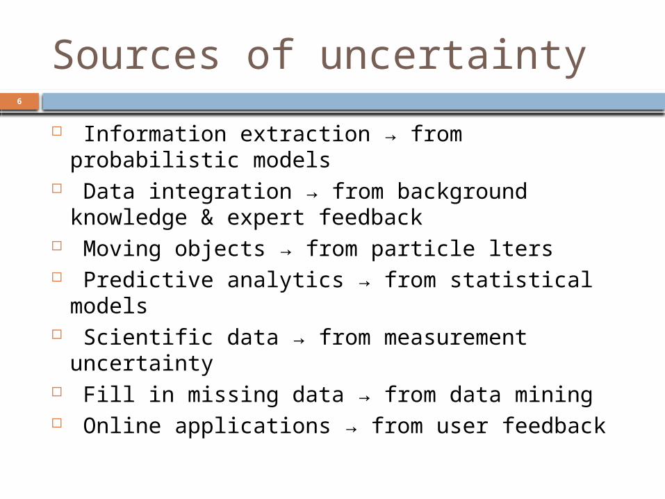
Sources of uncertainty

Information extraction → from probabilistic models

Data integration → from background knowledge & expert feedback

Moving objects → from particle lters Predictive analytics → from statistical models Scientific data → from measurement

uncertainty Fill in missing data → from data mining Online applications → from user feedback

7

Or-set tables

Name Bird Species

Besnik Bird-1 Finch: 0.8 || Toucan: 0.2

Niket Bird-2 Nightingale: 0.65 || Toucan: 0.35

Stephan Bird-3 Humming bird: 0.55 || Toucan: 0.45

t1t2

t3

Observed Species

Species

Finch (t1,1)

Toucan (t1,2) ˅(t2,2) ˅(t3,2)

Nightingale (t2,1)

Humming bird (t3,1)

Pc-table8

FID SSN Name

1 185 Smith X=1

1 785 Smith X≠1

2 185 Brown Y=1˄ X≠1

2 186 Brown Y ≠1 ˅ X = 1

V D P

X 1 0.2

X 2 0.8

Y 1 0.3

Y 2 0.7

FID

SSN Name

1 185 Smith

2 186 Brown

FID SSN Name

1 185 Smith

2 186 Brown

FID SSN Name

1 185 Smith

2 186 Brown{X→1, Y →1 }

{X→1, Y →2 }0.2×0.3+ 0.2×0.7=0.2

{X→2, Y →1 }0.8×0.3=0.24

{X→2, Y →2 }0.8×0.7=0.56

9

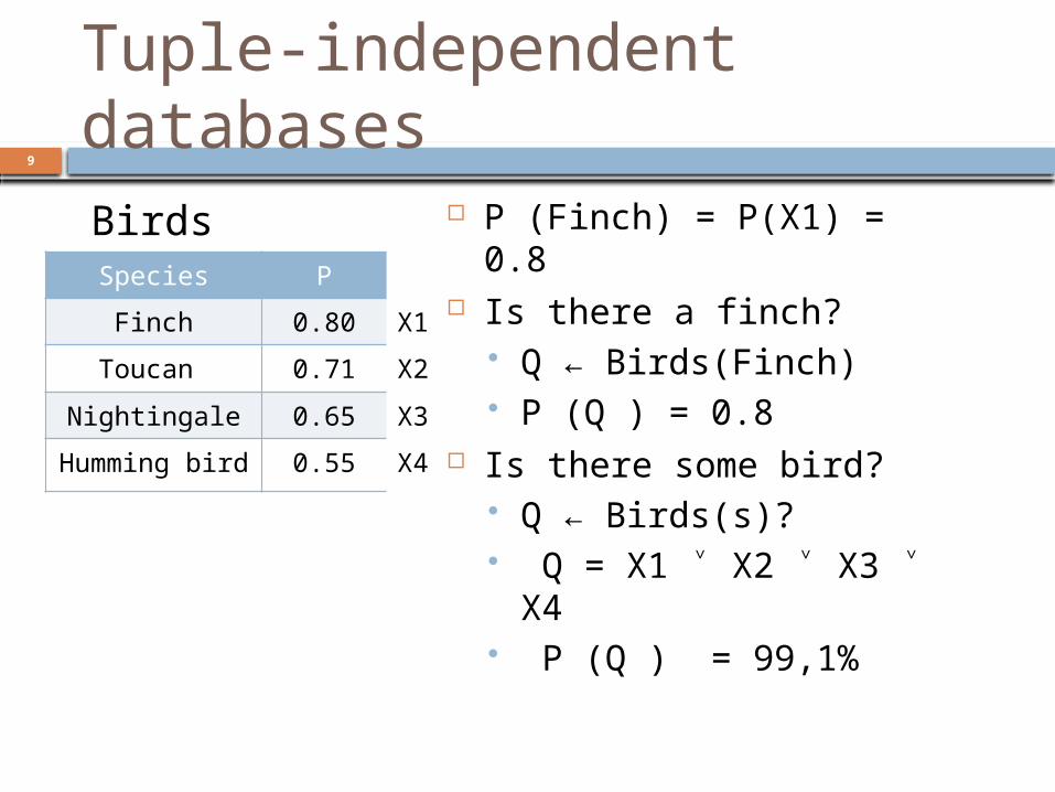
Tuple-independent databases

Species P

Finch 0.80 X1

Toucan 0.71 X2

Nightingale 0.65 X3

Humming bird 0.55 X4

Birds P (Finch) = P(X1) = 0.8 Is there a finch?

Q ← Birds(Finch) P (Q ) = 0.8

Is there some bird? Q ← Birds(s)? Q = X1 ˅ X2 ˅ X3 ˅ X4 P (Q ) = 99,1%

10

Outline




Evaluation

11

Semi-CRF

Input: sequence of tokens Output: segmentation s With a label Y consists of K attribute labels

And a special “Other”A probability distribution over s:

12

Semi-CRF

“52-A Goregaon West Mumbai PIN 400 062”

400 06252Goregao

nMumba

iPIN

Y1 Y4 Y5 Y6 Y7

West

A

Y2 Y3

CityAreaHouse_no ZipOther

13

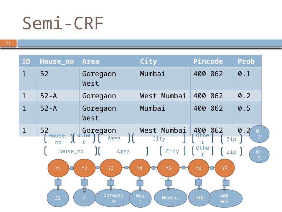
Semi-CRF

ID House_no

Area City Pincode Prob

1 52 Goregaon West

Mumbai 400 062 0.1

1 52-A Goregaon West Mumbai

400 062 0.2

1 52-A Goregaon West

Mumbai 400 062 0.5

1 52 Goregaon West Mumbai

400 062 0.2

400 06252Goregao

nMumba

iPIN

Y1 Y4 Y5 Y6 Y7

West

A

Y2 Y3

CityAreaHouse_no ZipOthe

r

CityAreaHouse_no Zip

Other

other

0.5

0.2

14

Number of segmentation required

15

Outline




Evaluation

16

Segmentation per row

ID House_no


1 52 Goregaon West

Mumbai 400 062 0.1


400 062 0.2


Mumbai 400 062 0.5


400 062 0.2

400 062

52Gorega

onMumbai

PIN

Y1 Y4 Y5 Y6 Y7

West

A

Y2 Y3

CityAreaHouse_no ZipOthe

r

CityAreaHouse_no Zip

Other

other

0.5

0.2

17

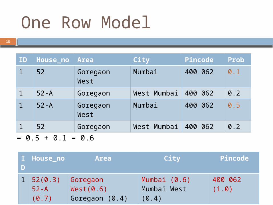
One Row Model

Let be probability for segment

Probability of the query

Pr((Area=‘Goregaon West’),City=‘Mumbai’) = 0.6×0.6 = 0.36

ID

House_no

Area City Pincode

1 52(0.3)52-A (0.7)

Goregaon West(0.6)Goregaon (0.4)

Mumbai (0.6)Mumbai West (0.4)

400 062 (1.0)

ID

House_no

Area City Pincode

1 52(0.3)52-A (0.7)



400 062 (1.0)

18

One Row Model

Pr((Area=‘Goregaon West’),City=‘Mumbai’)

= 0.5 + 0.1 = 0.6

ID House_no


1 52 Goregaon West

Mumbai 400 062 0.1


400 062 0.2


Mumbai 400 062 0.5


400 062 0.2

ID

House_no

Area City Pincode

1 52(0.3)52-A (0.7)



400 062 (1.0)

19

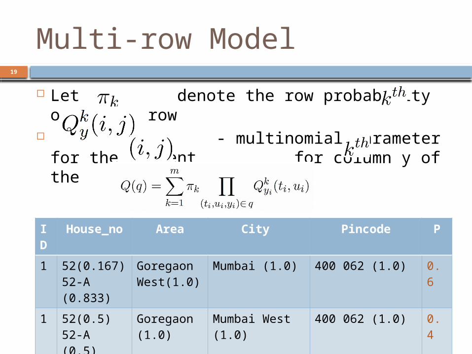
Multi-row Model

Let denote the row probability of row

- multinomial parameter for the segment for column y of the row

Pr((Area=‘Goregaon West’),City=‘Mumbai’) = 1*1*0.6+0*0*0.4 = 0.6

ID

House_no Area City Pincode P

1 52(0.167)52-A (0.833)

Goregaon West(1.0)

Mumbai (1.0) 400 062 (1.0) 0.6

1 52(0.5)52-A (0.5)

Goregaon (1.0)

Mumbai West (1.0)

400 062 (1.0) 0.4

20

Outline




Evaluation

21

Approximation Quality

Kullback–Leibler divergence

The parameters for One-Row model:

23

Computing Marginals

Forward pass: let be

Backward pass

Computing marginals:

24

Computing Marginals

S E

H_no

city

Zip

other

area

H_no

city

Zip

other

area

H_no

city

Zip

other

area

H_no

city

Zip

other

area

…∑(Pr) =

α

∑(Pr) = β

25

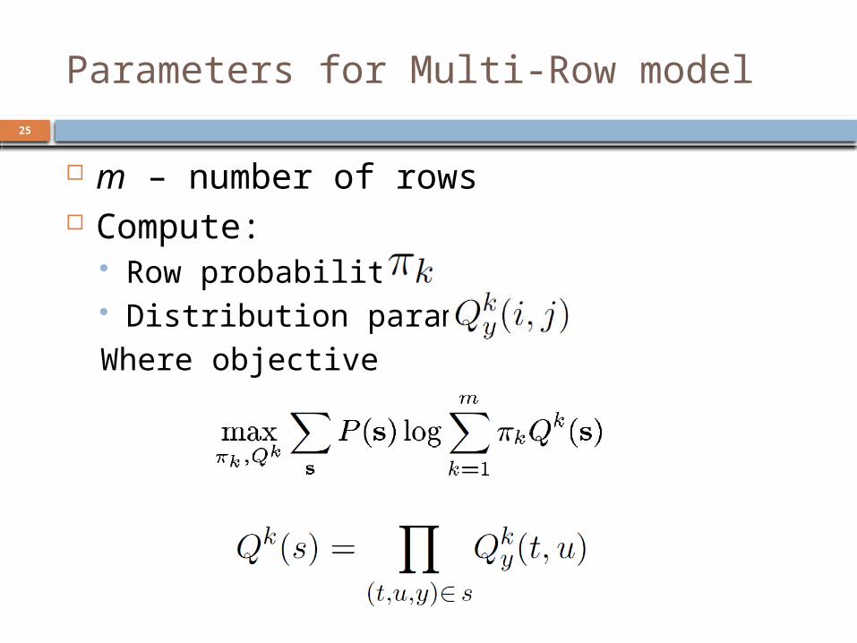
Parameters for Multi-Row model

m – number of rows Compute:

Row probabilities Distribution parametersWhere objective

26

Enumeration-based Approach Let be an enumeration of

all segments Objective

Expectation-Minimization algorithm E step M step

27

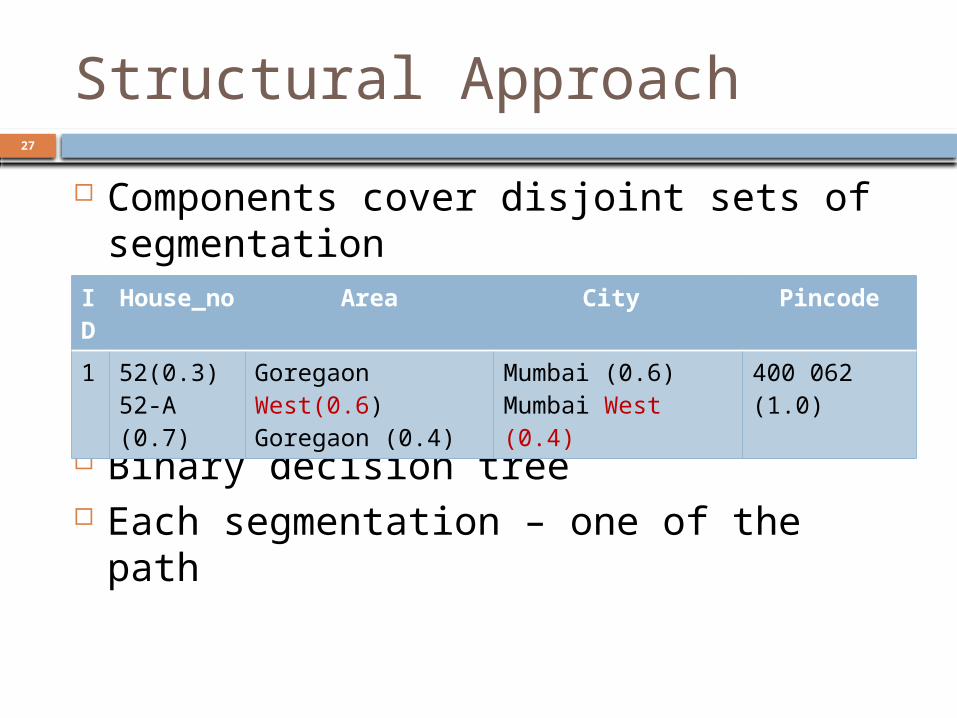
Structural Approach

Components cover disjoint sets of segmentation

Binary decision tree Each segmentation – one of the path

ID

House_no

Area City Pincode

1 52(0.3)52-A (0.7)



400 062 (1.0)

28

Structural Approach

Three kinds of variables:

For a given condition c entropy measure:

Information gain for

29

Computing parameters

S E

H_no

city

Zip

other

area

H_no

city

Zip

other

area

H_no

city

Zip

other

area

H_no

city

Zip

other

area

…∑(Pr) =

α

∑(Pr) = β

Under condition c

30

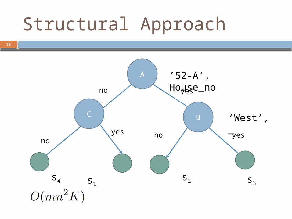
Structural Approach

A

B

s1

s2 s3

’52-A’, House_no

‘West’,_

yes

yesno

no

C

s4

yesno

31

Merging structures

Use E-M algorithm for all paths until converges: M-step

E-step Column of row are independent Each label defines a multinomial distribution

over it’s possible segments → generate one MD from another

32

Merging structures example

For disjoint segmentation:

s1= {‘52-A’, ‘Goregaon West’, ‘Mumbai’, 400062}s2= {’52’, ‘Goregaon’, ‘West Mumbai’, 400062}...

For m=2 rows:

R[1,s1] =0.2 R[1,s2] =0.1R[2,s2] =0.9 R[2,s1] =0.8

s1, s2 → row 2

ID

House_no

Area City Pincode

2 52-A(0.3)52 (0.7)


Mumbai (0.6)West Mumbai (0.4)

400 062 (1.0)

33

Outline




Evaluation

34

Evaluation

Two datasets Cora Address dataset

Strong(30%, 50%), Weak CRF (10%)

35

Comparing Models

Comparing divergence of 2 models with the same number of parameters

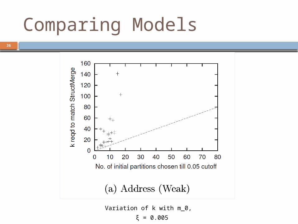
36

Comparing Models

Variation of k with m_0,

ξ = 0.005

37

Impact on Query Result

38

Impact on Query Result

Correlation between KL and inversion score. For StructMerge approach,

m=2, ξ = 0.005

39

Questions?

http://dilbert.com/strips/comic/2000-02-27/

40

References

1. Rahul Gupta, Sunita Sarawagi “Creating Probabilistic Databases from IE Models”

2. Reiner Gemulla, Lecture Notes of Scalable Uncertainty Management.

3. Wikipedia http://en.wikipedia.org/wiki/Kullback%E2%80%93Leibler_divergence

Creating Probabilistic Databases from IE Models Olga Mykytiuk, 21 July 2011 M.Theobald.

Documents

Transcript of Creating Probabilistic Databases from IE Models Olga Mykytiuk, 21 July 2011 M.Theobald.