and Watkins). We thank

comments and discussions. We are

NBER WORKING PAPER SERIES

CREATING MOVES TO OPPORTUNITY:EXPERIMENTAL EVIDENCE ON BARRIERS TO NEIGHBORHOOD CHOICE

Peter BergmanRaj Chetty

Stefanie DeLucaNathaniel HendrenLawrence F. KatzChristopher Palmer

Working Paper 26164

http://www.nber.org/papers/w26164NATIONAL BUREAU OF ECONOMIC RESEARCH

1050 Massachusetts AvenueCambridge, MA 02138

August 2019, revised March 2020

We are grateful to our partners who implemented the experiment analyzed in this paper: the Seattle and King County Housing Authorities (especially Andria Lazaga, Jenny Le, Sarah Oppenheimer, and Jodell Speer), MDRC (especially Gilda Azurdia, Jonathan Bigelow, David Greenberg, James Riccio, and Nandita Verma), and J-PAL North America (especially Jacob Binder, Graham Simpson, and Kristen Watkins). We thank Isaiah Andrews, Ingrid Gould Ellen, John Friedman, Edward Glaeser, Scott Kominers, Katherine O'Regan, Maisy Wong, Abigail Wozniak, and numerous seminar participants for helpful comments and discussions. We are indebted to Michael Droste, Federico Gonzalez Rodriguez, Jamie Gracie, Kai Matheson, Martin Koenen, Sarah Merchant, Max Pienkny, Peter Ruhm, James Stratton, and other Opportunity Insights pre-doctoral fellows for their outstanding contributions to this work, as well as the Johns Hopkins based fieldwork team who helped collect interviews, including: Paige Ackman, Christina Ambrosino, Divya Baron, Joseph Boselovic, Erin Carll, Devin Collins, Hannah Curtis, Christine Jang, Akanksha Jayanthi, Nicole Kovski, Melanie Nadon, Kiara Nerenberg, Daphne Moraga, Bronte Nevins, Elise Omaki, Simone Robbennolt, Brianna So, Jasmine Sausedo, Sydney Thomas, Maria Vignau-Loria, Allison Young, andMEF Associates. This research was funded by the Bill & Melinda Gates Foundation, Chan-Zuckerberg Initiative, Surgo Foundation, the William T. Grant Foundation, and Harvard University. This project and a pre-analysis plan were preregistered with the AEA RCT Registry (AEARCTR-0002807). This study was approved under Harvard Institutional Review Board IRB18-1573, MDRC IRB 1030056-4, and Johns Hopkins University HIRB 00001010. The views expressed herein are those of the authors and do not necessarily reflect the views of the National Bureau of Economic Research.

NBER working papers are circulated for discussion and comment purposes. They have not been peer-reviewed or been subject to the review by the NBER Board of Directors that accompanies official NBER publications.

© 2019 by Peter Bergman, Raj Chetty, Stefanie DeLuca, Nathaniel Hendren, Lawrence F. Katz, and Christopher Palmer. All rights reserved. Short sections of text, not to exceed two paragraphs, may be quoted without explicit permission provided that full credit, including © notice, is given to the source.

A randomized controlled trials registry entry is available at https://www.socialscienceregistry.org/trials/2807Video Summary of Study Findingshttps://www.youtube.com/watch?v=w8hHtk7oe1w&feature=youtu.be

Creating Moves to Opportunity: Experimental Evidence on Barriers to Neighborhood Choice Peter Bergman, Raj Chetty, Stefanie DeLuca, Nathaniel Hendren, Lawrence F. Katz, and Christopher PalmerNBER Working Paper No. 26164August 2019, revised March 2020JEL No. H0,J0,R0

ABSTRACT

Low-income families in the United States tend to live in neighborhoods that offer limited opportunities for upward income mobility. One potential explanation for this pattern is that families prefer such neighborhoods for other reasons, such as affordability or proximity to family and jobs. An alternative explanation is that they do not move to high-opportunity areas because of barriers that prevent them from making such moves. We test between these two explanations using a randomized controlled trial with housing voucher recipients in Seattle and King County. We provided services to reduce barriers to moving to high-upward-mobility neighborhoods: customized search assistance, landlord engagement, and short-term financial assistance. Unlike many previous housing mobility programs, families using vouchers were not required to move to a high-opportunity neighborhood to receive a voucher. The intervention increased the fraction of families who moved to high-upward-mobility areas from 15% in the control group to 53% in the treatment group. Families induced to move to higher opportunity areas by the treatment do not make sacrifices on other aspects of neighborhood quality, tend to stay in their new neighborhoods when their leases come up for renewal, and report higher levels of neighborhood satisfaction after moving. These findings imply that most low-income families do not have a strong preference to stay in low-opportunity areas; instead, barriers in the housing search process are a central driver of residential segregation by income. Interviews with families reveal that the capacity to address each family's needs in a specific manner — from emotional support to brokering with landlords to customized financial assistance — was critical to the program's success. Using quasi-experimental analyses and comparisons to other studies, we show that more standardized policies — increasing voucher payment standards in high-opportunity areas or informational interventions — have much smaller impacts. We conclude that redesigning affordable housing policies to provide customized assistance in housing search could reduce residential segregation and increase upward mobility substantially.

Peter Bergman Columbia University 525 W. 120th StreetBox 174New York, NY 10027 bergman@tc.columbia.edu

Raj ChettyDepartment of Economics Harvard University

Littauer 321Cambridge, MA 02138A and NBERchetty@fas.harvard.edu

Stefanie DeLucaJohns Hopkins University Department of Sociology sdeluca@jhu.edu

Nathaniel Hendren Harvard University Department of Economics Littauer Center Room 235 Cambridge, MA 02138 and NBERnhendren@gmail.com

Lawrence F. Katz Department of EconomicsHarvard University Cambridge, MA 02138 and NBERlkatz@harvard.edu

Christopher Palmer MIT Sloan School of Management 100 Main Street, E62-639 Cambridge, MA 02142 and NBERcjpalmer@mit.edu

youtu.be

I Introduction

Recent research has established that children’s outcomes in adulthood vary substantially across

neighborhoods and that moving to higher opportunity neighborhoods earlier in childhood improves

children’s outcomes significantly (Chetty, Hendren, and Katz 2016; Chetty and Hendren 2018a;

Chyn 2018; Laliberte 2018). Yet the vast majority of low-income families in the United States,

including those receiving Housing Choice Vouchers from the government, live in low-opportunity

neighborhoods (Metzger 2014; Mazzara and Knudsen 2019). This pattern prevails even though

many families live near areas with similar or lower rental costs that historically have produced

much better economic outcomes for children (Chetty et al. 2018). Why don’t more low-income

families take advantage of these options and move to opportunity? More broadly, what explains

the segregation of low-income families into high-poverty, low-opportunity neighborhoods in many

cities?

One potential explanation is that low-income families prefer to stay in low-opportunity areas

because these neighborhoods have other valuable amenities, such as shorter commutes, proximity

to family and community, or greater racial and ethnic diversity. An alternative explanation is

that low-income families do not move to high-opportunity areas because of barriers, such as a lack

of information, frictions in the search process (e.g., a lack of credit or liquidity), or a reluctance

among landlords to rent to them. Distinguishing between these two explanations is important

for understanding the drivers of residential segregation as well as for designing affordable housing

policies to address any barriers that limit moves to opportunity.1

We test between these explanations using a randomized controlled trial, implemented in collab-

oration with the Seattle and King County housing authorities, that sought to reduce the barriers

families may face in moving to higher opportunity areas. The trial involved 430 families who applied

for and were issued Housing Choice Vouchers, which provide $1,540 per month in rental assistance

on average to eligible low-income families. The sample consisted of families with a child below age

15 issued vouchers between April 2018 and April 2019 in the Seattle and King County area, who

had a median household income of $19,000.

We began by defining “high-opportunity” neighborhoods as Census tracts that have historical

rates of upward income mobility in approximately the top third of tracts in the Seattle and King

County area, drawing on data from a preliminary version of the Opportunity Atlas. On aver-

1. An extensive literature in sociology and economics has studied the determinants of residential choice and segre-gation over the past fifty years. We discuss how our study contributes to this literature at the end of the introduction.

1

age, children who grow up in low-income (25th percentile) families in the areas we designated as

“high opportunity” earn about 13.9% ($6,800 per year) more as adults than those who grow up in

low-opportunity areas in families with comparable incomes. Historically, around 12% of voucher

recipients in Seattle and King County leased units in the areas we define as high opportunity.

Families who applied for housing vouchers were randomly assigned (with 50% probability) to a

control group or treatment group. The value of the vouchers and the restrictions governing their

use followed pre-existing housing authority regulations and did not differ between the treatment

and control groups. Families in the control group received standard briefings on how to use their

vouchers. Families in the treatment group were offered a supplementary program designed to help

them lease units in high-opportunity areas called Creating Moves to Opportunity (CMTO). The

CMTO program consisted of three components: customized search assistance, landlord engage-

ment, and short-term financial assistance. The total cost of the program was about $2,660 per

family.2 Search assistance was provided by a non-profit group and included information about

high-opportunity areas, assistance in preparing rental documents, guidance in addressing issues in

a family’s credit and rental history, and help in identifying available units and connecting with

landlords in high-opportunity areas. On average, CMTO staff spent about six hours working with

each family. The staff also engaged directly with landlords in opportunity areas to encourage them

to lease units to CMTO families and expedite the lease-up process. Landlords who leased to CMTO

families were additionally offered an insurance fund for damages to the unit above and beyond the

security deposit. Finally, financial assistance included funds administered by the program staff

for security deposits and application fees, averaging $1,000 per family. Importantly, all families in

the treatment group had the option to use their housing voucher in any neighborhood within the

housing authorities’ jurisdictions (although CMTO services were only provided in high-opportunity

areas).3

The CMTO treatment increased the share of families who leased units in high-opportunity

neighborhoods by 37.9 percentage points (s.e. = 4.2 pp, p < 0.001), from 15.1% in the control

2. This $2,660 figure is the up-front cost of the program services; it excludes downstream costs incurred in theform of higher housing voucher payments that were incurred by housing authorities because treatment group familiesmoved to more expensive neighborhoods. See Section III.C for details.

3. This element of neighborhood choice is the critical distinction between CMTO and the Moving to Opportunity(MTO) experiment implemented in the 1990s, which required that families in the experimental group move to low-poverty Census tracts to receive a voucher. Studies of the MTO experiment have shown that families who moved tohigher-opportunity areas as required by the experimental treatment had improved mental health and well-being andbetter economic outcomes for their children (Kling, Liebman, and Katz 2007; Chetty, Hendren, and Katz 2016; Ludwiget al. 2012). The focus of the CMTO experiment is on why families receiving vouchers without such requirementstypically do not live in such areas.

2

group to 53.0% in the treatment group. We find similarly large treatment effects on moves to high-

opportunity areas across several subgroups, including racial minorities, immigrant families, and

the lowest-income households in the sample. CMTO changed where families moved, not whether

they moved at all with a Housing Choice Voucher: in both the treatment and control groups,

approximately 87% of families leased a unit somewhere using their housing vouchers. The fact that

families are able to use their vouchers to find housing at similar rates even without CMTO services

shows that the program did not induce families to move to high-opportunity areas simply to use

their vouchers; rather, it expanded families’ neighborhood choice sets.

Families in the treatment group moved to many different Census tracts across the Seattle and

King County area: the 118 families in the treatment group who moved to a high-opportunity area

live in 46 different tracts, mitigating the concern that the program might simply reconcentrate

low-income families in new neighborhoods (Clark 2008). Families who moved to high-opportunity

areas chose neighborhoods whose characteristics are representative of high-opportunity areas over-

all, which tend to have lower poverty rates, higher shares of two-parent families, slightly lower

shares of non-white residents, and lower population density. Families who moved to opportunity

did not gravitate to lower-opportunity areas within the set of neighborhoods designated as“high op-

portunity”; in fact, several families moved to the highest-upward-mobility neighborhoods in Seattle

and King County.

Families induced to move to high-opportunity areas by the CMTO treatment tend to stay in

higher-opportunity areas when their leases come up for renewal (one year after their initial move).

Among families who leased up at least one year earlier, 60.0% of families in the treatment group live

in high-opportunity areas, compared with 19.1% in the control group. These rates are almost the

same as those observed at initial lease up, showing that the treatment effect on neighborhood choice

is highly persistent over one year. Furthermore, in a post-move survey of a randomly selected subset

of families, families in the treatment group express higher rates of neighborhood satisfaction and a

greater likelihood of wanting to stay in their new neighborhoods. For instance, 64.2% of families

in the treatment group report being “very satisfied” with their new neighborhood, compared with

45.5% in the control group. These findings suggest that families in the treatment group are likely

to remain in high-opportunity areas in the long run.

Families who moved to high-opportunity areas do not appear to have made sacrifices on other

observable neighborhood amenities, such as distance to their prior location or proximity to jobs,

nor in the quality of the unit they rent, as measured by its size, age, or other characteristics.

3

This may be because Seattle and King County had a tiered payment standard for vouchers that

offered higher payments for more expensive neighborhoods (a policy introduced independently of

the CMTO experiment), allowing families to access more expensive units in high-opportunity areas.

Indeed, the average monthly rent was $188 higher for families assigned to the CMTO treatment

group than the control.

Our experimental results imply that most low-income families do not have a strong preference

to stay in low-opportunity areas; rather, barriers to moving to high-opportunity areas play a central

role in explaining neighborhood choice and residential sorting patterns. Explaining our findings with

a frictionless model in which neighborhood choices are determined purely by preferences would

require that a large group of families happen to be close to indifferent between low- and high-

opportunity areas. In particular, our treatment effect estimates conditional on leasing up imply

that 43% of families must have a willingness to pay (WTP) to live in a low-opportunity area between

$0 and $2,660 (the per-family cost of the CMTO program).4 This is implausible both because we

find uniformly large treatment effects across subgroups and because the marginal families induced

to move to high-opportunity areas by the intervention report much higher levels of neighborhood

satisfaction after moving.5 A more plausible explanation of the data is that many low-income

families have strong preferences to move to high-opportunity areas, but are prevented from doing

so by barriers in the search process. Such barriers could potentially be captured in a reduced-

form manner by incorporating sufficiently large housing search costs into the model (e.g., Wheaton

1990; Kennan and Walker 2011), but unpacking what these search costs are is critical for developing

policies that could reduce these costs and help families find housing in their preferred neighborhoods.

To understand the barriers families face and the mechanisms through which CMTO addressed

them, we conducted 161 in-depth (on average, two hour) interviews with a stratified random sample

of families in the treatment and control groups during and after their move. Many families reported

that they had limited time and resources to search for housing, as they were facing challenges such

as domestic violence, mental health conditions, or holding multiple jobs while caring for children as

single parents. Families identified five key mechanisms through which the CMTO program helped

them move to opportunity: providing emotional support, increasing motivation to move to a high-

opportunity neighborhood, streamlining the search process by helping to prepare rental applications

4. Adding the 18% who move to opportunity in the control group implies that a majority of the population iswilling to pay at most $2,660 to live in a low-opportunity area.

5. Similar reasoning suggests that the scarcity of voucher holders in high-opportunity areas is also unlikely to bedue to strong preferences for non-voucher holders among landlords. In particular, any such preference must be smallenough to be overcome by the CMTO treatment for a large fraction of landlords.

4

and “rental resumes,” providing direct brokerage services and representation with landlords, and

providing crucial and timely assistance for auxiliary payments that could prevent a lease from

being signed. The qualitative interviews show that the CMTO program’s ability to respond to each

family’s specific needs and circumstances was critical to the program’s impact. Service utilization

was highly heterogeneous across families, with some families relying heavily on search assistance,

while others used more financial assistance or took advantage of direct landlord referrals.

Consistent with the importance of customized services, we find that CMTO increased access

to high-opportunity neighborhoods substantially more than other more standardized policies with

similar goals. One prominent approach, termed Small Area Fair Market Rents, is to provide

financial incentives to help families move to higher-opportunity neighborhoods by offering higher

voucher payment standards in higher-rent ZIP codes within a metro area (HUD 2016). The King

County Housing Authority implemented such a policy in March, 2016. Using a quasi-experimental

difference-in-differences design comparing voucher recipients in Seattle vs. King County, we find

that King County’s change in payment standards had little or no impact on the rate of moves to

high-opportunity areas, with an upper bound on the 95% confidence interval of a 7.7 pp increase

– an order of magnitude lower than the effects of CMTO. We also study a policy introduced by

the Seattle Housing Authority that increased payment standards specifically in high-opportunity

neighborhoods (as designated for the CMTO experiment). Again, we find it had a much smaller

impact on the rates of moves to high-opportunity areas. Indeed, only 20% of voucher recipients

with children moved to high-opportunity areas even after these changes in payment standards were

implemented. These findings show that financial incentives are insufficient to induce a high rate

of moves to opportunity by themselves (although they may be necessary to facilitate such moves

through CMTO-style programs, especially in expensive housing markets).6

Another alternative to customized housing search assistance is to provide information in a

lower-cost, more standardized manner. Schwartz, Mihaly, and Gala (2017) report results from a

randomized trial showing that short-run financial incentives and light-touch counseling had little

impact on the rate of moves to higher opportunity areas in Chicago. Bergman, Chan, and Kapor

(2019) randomized the provision of information to families about the quality of schools associated

with rental units on a website commonly used by voucher holders. The information intervention

resulted in moves to units with slightly better neighborhood schools, but had a much smaller impact

6. Of course, there are many potential goals of affordable housing beyond increasing upward mobility for children,such as providing safe and stable shelter or shorter commutes. Small Area Fair Market Rents could be valuable inachieving these other objectives; our results do not speak to such considerations.

5

on neighborhood quality than CMTO. Moreover, CMTO greatly increased (by 48 percentage points)

the fraction of families who stayed in high-opportunity areas even among those who were living in

high-opportunity neighborhoods when they applied for vouchers – families who were presumably

informed about those areas. Furthermore, 72% of families felt“good”or“very good”about moving to

an opportunity neighborhood even at the point of the baseline survey, before the CMTO intervention

began. These results all suggest that information alone does not drive CMTO’s impacts and is

unlikely to greatly increase moves to opportunity areas by itself.

From a policy perspective, our results imply that redesigning affordable housing programs to

facilitate more moves to opportunity could have substantial impacts on residential segregation and

intergenerational income mobility. Using data from Chetty et al. (2018), we estimate that the moves

from low- to high-opportunity Census tracts induced by CMTO will increase average undiscounted

lifetime household incomes by $214,000 (8.4%) for children who move at birth and stay in their new

neighborhoods throughout childhood. More broadly, given that low-income families do not have

strong preferences for low-opportunity neighborhoods, our results provide support for increasing

the availability of affordable housing in higher-opportunity areas through other policies such as the

Low Income Housing Tax Credit, project-based units, or changes in zoning regulations.

Although our findings are encouraging for mobility programs that facilitate residential choice,

two important caveats should be kept in mind. First, general equilibrium effects could dampen the

causal impacts of neighborhoods when families move in or out of them. In practice, the families in

CMTO came from a wide variety of neighborhoods and, as noted above, moved to a wide variety of

different areas. This dispersion suggests that CMTO (or even scaled-up versions of the program)

will not change the characteristics of any neighborhood sufficiently to dampen the benefits of moving

to higher opportunity areas. Moreover, most of the families who moved to a high-opportunity area

in the CMTO program would have moved to some other neighborhood even absent these services,

implying that CMTO does not have any incremental effect on destabilizing the neighborhoods

where families were initially living.7

7. If the supply of housing units in each neighborhood is fixed, as is likely the case in the short run, the familiesinduced to move to opportunity by CMTO must displace other families from high-opportunity areas, thereby reducingthe aggregate gains from the program. Since the average voucher holder has a lower income than the averagefamily living a high-opportunity area, expanding CMTO would increase the share of low-income families relative tohigh-income families in high-opportunity neighborhoods. Such reallocations could increase aggregate income sinceneighborhoods appear to matter less for the outcomes of children in higher-income families (Chetty et al. 2018) and,irrespective of their impacts on total income, may be desirable from a distributional perspective. In the long run, thesupply of housing may expand in response to increases in demand in high-opportunity areas induced by the CMTOprogram. These general equilibrium effects could be quantified following the methods developed in Galiani, Murphy,and Pantano (2015), Davis, Gregory, and Hartley (2018), and Davis et al. (2017).

6

Second, it remains to be seen whether the findings reported here for the Seattle and King

County area generalize to other housing markets. On the one hand, Seattle and King County are

tight housing markets in which high-opportunity areas have little affordable housing, suggesting

treatment effects could be even larger elsewhere. On the other hand, Seattle may be a market that

is conducive to opportunity moves, as it bans source-of-payment discrimination and has other char-

acteristics that may make it easier for lower-income families to find housing in higher-opportunity

areas. We hope that other public housing authorities will be able to test similar programs elsewhere,

perhaps in the context of the Housing Choice Voucher Mobility Demonstration.

This paper builds on an extensive literature in sociology and economics that has analyzed the

role of preferences versus structural barriers as causes of segregation (e.g., Schelling 1971; Kain

and Quigley 1975; D. Massey and N. Denton 1987; Sampson 2012; Sharkey 2013; Lareau and

Goyette 2014; Krysan and Crowder 2017). Much of this work has focused on racial segregation,

highlighting the importance of forces such as discrimination (Yinger 1995; Turner et al. 2013) and a

lack of information (Krysan and Bader 2009) in producing segregation despite African Americans’

preferences for living in more integrated neighborhoods (e.g. Charles 2005; Emerson, Chai, and

Yancey 2001). A smaller body of work has examined the drivers of socioeconomic segregation (e.g.,

Reardon and Bischoff 2011), which is our primary focus here. Our contributions to this literature

are (1) establishing experimentally that barriers have substantial causal effects on neighborhood

choice among low-income families; (2) characterizing the barriers at play, showing in particular that

they extend beyond racial discrimination, a lack of information, or a lack of financial liquidity and

instead involve deeper psychological and sociological constraints; and (3) demonstrating that these

barriers can be reduced through feasible modifications of existing government programs.

The paper is organized as follows. Section II summarizes a set of facts on the geography

and price of opportunity in Seattle and King County that motivate our intervention. Section III

provides institutional background on the housing voucher program and describes our intervention

and experimental design. Section IV describes the data we use. Section V reports the experimental

results and interprets their implications using a stylized model of neighborhood choice. Section VI

presents qualitative evidence on mechanisms. In Section VII, we compare the effects of CMTO to

other policies, including changes in payment standards and informational interventions. Section

VIII concludes.

7

II The Geography and Price of Opportunity in Seattle

In this section, we summarize four facts on the geography and price of opportunity that motivate

our intervention.8

First, children’s rates of upward income mobility vary substantially across nearby tracts. Figure

1a plots upward income mobility by Census tract in King County (which includes the city of Seattle

and surrounding suburbs) using data from the Opportunity Atlas (Chetty et al. 2018). The map

shows the average household income percentile rank at age 35 for children who grew up in low-

income (25th percentile) families in the 1978-1983 birth cohorts.9 There is substantial variation

in upward mobility across tracts: the (population-weighted) standard deviation of children’s mean

income ranks in adulthood across tracts within King County is 4.7 percentiles (approximately

$5,175, or 10.3% of mean annual income for children with parents at the 25th percentile).

Second, much of the variation in upward mobility across neighborhoods is driven by the causal

effects of childhood exposure rather than sorting. Recent studies have established that moving to

high-upward-mobility (“high-opportunity”) neighborhoods improves children’s outcomes in adult-

hood in proportion to the amount of time they spend growing up there. These studies, summarized

in Appendix Figure 1, use research designs ranging from random assignment of vouchers (Chetty,

Hendren, and Katz 2016) and quasi-experimental estimates based on variation in the age of chil-

dren at the time of the move (Chetty et al. 2018; Laliberte 2018) to demolitions of public housing

projects (Chyn 2018). They find that approximately two-thirds of the observational variation in

upward mobility across tracts is due to causal effects of place.

Third, low-income families are concentrated in lower-opportunity neighborhoods. Even among

families that receive rental assistance from the government in the form of housing vouchers, 76.2%

of families in Seattle and King County live in tracts with below-median levels of upward mobility.

Figure 1a illustrates this fact by showing the 25 most common locations where families with housing

vouchers moved between 2015 and 2017 (as a percentage of the total population in each tract).

Families are clustered in lower-opportunity tracts (red colors) even though there are often much

higher-opportunity tracts nearby.

Fourth, the segregation of low-income families into low-opportunity areas is not simply explained

by differences in the price of housing between low- and high-opportunity neighborhoods. Figure

8. We establish these facts using data from Seattle and King County here, but the same four facts hold systemat-ically in other metro areas across the country.

9. Children are assigned to tracts in proportion to the number of years they spent growing up in that tract untilage 23; see Chetty et al. (2018) for further details.

8

1b plots the upward mobility measure shown in Figure 1a against median rent for a two-bedroom

apartment in each tract, using data from the 2012-2015 American Community Survey (ACS) to

measure rents. Neighborhoods with higher upward mobility are slightly more expensive: the (low-

income count-weighted) correlation between rents and upward mobility is 0.24 within King County.

However, there is considerable variation in upward mobility even conditional on rent. Figure 1b

highlights the most common tracts where voucher holders lived prior to our experimental interven-

tion and shows that many families could potentially move to “opportunity bargain” neighborhoods

that would improve their children’s outcomes without having higher rents.10

These four facts motivate our central questions: Why don’t more low-income families, especially

those receiving housing vouchers, move to opportunity? Do families prefer lower-opportunity areas

because they have other advantages (e.g., a shorter commute to work or proximity to family)? Or

do they prefer higher-opportunity neighborhoods, but face barriers that limit access to such areas?

If families face such barriers, how can we intervene to help families live where they would like to

live?

III Intervention and Experimental Design

In this section, we describe our intervention and experimental design. We begin by providing

some institutional background on the Housing Choice Voucher (HCV) program. We then discuss

our definition of high-opportunity neighborhoods, the services offered in the Creating Moves to

Opportunity program, and the design of the randomized controlled trial.

III.A Background on the Housing Choice Voucher Program

The HCV program provides rental assistance to 2.2 million families in the United States each year,

with a total program cost of approximately $20 billion annually (see Collinson, Ellen, and Ludwig

(2015) for a comprehensive description of the program). The program is overseen at the federal

level by the U.S. Department of Housing and Urban Development (HUD), but is administered by

local Public Housing Authorities (PHAs). In this study, we work with two PHAs: the Seattle

Housing Authority (SHA), which issues vouchers that can be used in the city of Seattle, and the

King County Housing Authority (KCHA), which issues vouchers that can be used in the rest of

10. Moreover, the housing authorities offer tiered payments standards such that families receive more rental assis-tance if they find housing in a more expensive area, further reducing the effective cost of housing in high-opportunityneighborhoods.

9

King County, excluding the cities of Seattle and Renton.11 Both KCHA and SHA are among a

small number of PHAs who participate in HUD’s Moving to Work program, which gives them

greater flexibility to implement policy pilots than other PHAs.

The HCV program is targeted at low-income families. To be eligible for a voucher from SHA

and KCHA, families must have household income below 80% of Area Median Income (AMI).12 In

line with national patterns, more families meet this criteria than the number of vouchers available.

The PHAs address this problem by using a lottery to assign families positions on a waiting list.

Families who are homeless or who have incomes below 30% of AMI are given priority on the waitlist.

In practice, virtually all families who actually receive vouchers fall well below the 30% AMI cutoff,

which corresponds to $29,900 for a family of 3. In Seattle and King County, the typical family who

received a voucher during our experiment had been on the waitlist for about 1.5 years.

Families eligible for the HCV program are required to contribute 30 to 40% of their annual

household income toward rent and utilities. They then receive a housing subsidy that covers the

difference between a unit’s listed rent and the family’s contribution, up to a maximum amount

known as the Voucher Payment Standard. In SHA and KCHA, the maximum monthly voucher

payments for a two-bedroom unit were $2278 and $2110, respectively.13

Once families are issued a voucher, they typically have 4 to 8 months to use the voucher to lease

a unit; if the voucher is not used by that point, it is issued to another family. To use a voucher,

families must find an interested landlord whose unit passes a quality inspection conducted by the

PHA using HUD-defined housing quality standards. After leasing, families remain eligible for the

voucher they received indefinitely as long their income remains below eligibility thresholds.

III.B Defining Opportunity Areas

The first step in our intervention is to designate which areas are “high-opportunity” neighborhoods.

Using a preliminary version of the Opportunity Atlas data on upward mobility shown in Figure

1a, we define high-opportunity neighborhoods as Census tracts that have upward mobility in ap-

proximately the top third of the distribution across tracts within Seattle and King County.14 We

11. Vouchers from both SHA and KCHA may be ported out to use in other areas if they meet certain requirements;this occurs relatively infrequently in practice.

12. Families must also meet certain additional requirements, such as having children or meeting certain age require-ments. The full set of requirements are available here for SHA and here for KCHA.

13. In recent years, both SHA and KCHA have adopted tiered payment standards that offer higher payments inmore expensive areas to enable families to move to more expensive neighborhoods.

14. We describe the procedure used to construct the preliminary measures of upward mobility in Appendix A.Appendix Figure 2 compares the preliminary estimates to the final Opportunity Atlas estimates shown in Figure 1a(which were released in October 2018) and shows that they are quite similar in practice, with a correlation of 0.74

10

then adjust these definitions to (1) create contiguous areas and (2) account for potential neighbor-

hood change.15 We create contiguous areas by including Census tracts that fall below the “high

opportunity” threshold according to their upward mobility estimates but are surrounded by other

high-opportunity areas and excluding high-opportunity Census tracts that are surrounded only by

lower-opportunity neighborhoods (see Appendix A for details).

We address neighborhood change by evaluating whether the historical measures of upward

mobility in the Opportunity Atlas – which are constructed using data for children who grew up in

these areas in the 1980s and 1990s – are good predictors of opportunity for children growing up in

those areas today. Chetty et al. (2018) examine the serial correlation of upward mobility measures

across cohorts. They find that rates of upward mobility are generally quite stable over time and

that historical mobility is more predictive of future mobility than typical contemporaneous proxies

for opportunity, such as poverty rates. That said, there are certain parts of Seattle, especially near

the center of the city, which have gentrified dramatically in the past ten years and could potentially

have very different outcomes today. To evaluate the impacts of this change, we examine the test

scores of low-income (free-lunch-eligible) students living in these areas, a plausible leading indicator

of upward income mobility. The test-scores of low-income students did not change significantly in

these areas (although average test scores, pooling all income groups, increased as higher-income

families moved in). We conclude based on this analysis that the historical Opportunity Atlas

measures provide good predictors of opportunity for low-income families even in these changing

neighborhoods.16 Based on these and other qualitative analyses by the housing authorities, we

chose to proceed with the designations largely based on the Opportunity Atlas data.

Figure 2a shows the final set of Census tracts that were designated as “high opportunity” (in the

dark shading) after this process. These definitions of high-opportunity areas differ from previous

definitions used by SHA and KCHA as well as other practitioners and researchers. Most prior

studies define “high-opportunity” areas based on proxies such as the availability of jobs, transit

access, crime rates, poverty rates, etc. In contrast, we directly define high-opportunity areas as

places where low-income children have had good outcomes historically. We focus on children because

prior work has shown that neighborhoods have the largest impacts on children’s rather than adults’

across tracts in King County.15. We also excluded three high-opportunity tracts that already had a large concentration of voucher holders, based

on the reasoning that the barriers families face in moving to these areas were already low.16. Of course, there is no guarantee that this will be the case in other areas where neighborhoods have changed

substantially. The Opportunity Atlas data provide a good starting point for predicting upward mobility (which isinherently unobservable) for the current generation of children, but should ideally be complemented with more recentdata and qualitative judgment on a case-by-case basis to settle on final definitions of opportunity neighborhoods.

11

economic outcomes. We focus on their outcomes rather than proxies for those outcomes because

prior work has shown that observable characteristics such as poverty rates capture only about 50%

of the variation in upward mobility across areas.

Figure 2b shows why this distinction matters in practice. The left panel replicates the Op-

portunity Atlas data from Figure 1a, while the right panel shows the Kirwan Child Opportunity

Index (Acevedo-Garcia et al. 2014), a commonly used index constructed by combining education,

health, and economic indicators. The two measures have a (population-weighted) correlation of

0.3, leading to several important differences between them. For example, the Kirwan index ranks

Capitol Hill and parts of the Ballard neighborhood as high-opportunity areas (given their proximity

to jobs), yet these neighborhoods have historically had some of the lowest rates of upward mobility

in Seattle. Conversely, there are several areas, such as the eastern part of Kent in King County

and the Northeastern part of Seattle, which rate poorly according to the Kirwan index but offer

high rates of upward income mobility for low-income children. Such areas often excel on other

dimensions that are correlated with upward mobility, such as measures of social capital and family

stability, which are typically not incorporated into traditional measures.

Helping families move to high-opportunity areas as defined based on the Opportunity Atlas

rather than traditional Kirwan or poverty-rate-based indices is likely to produce larger impacts

on upward income mobility for two reasons. First, we estimate that the average high-opportunity

area identified as described above using the Opportunity Atlas has a causal effect on upward

income mobility that is nearly 40% larger than what one would have obtained if one identified

the same number of high-opportunity tracts based on the Kirwan index or poverty rates. Second,

neighborhoods that have high rates of upward mobility despite appearing worse on observable

dimensions tend to have lower rents (Chetty et al. 2018). As a result, our designation of high-

opportunity areas identifies more affordable neighborhoods than traditional Kirwan-type or poverty-

rate-based indices, expanding the set of high-opportunity areas that would be affordable to families

receiving vouchers.17

III.C The Creating Moves to Opportunity Intervention

In collaboration with our research team, the Seattle and King County Housing Authorities devel-

oped a suite of services designed to facilitate moves to high-opportunity neighborhoods, building on

17. Only 36% of the families who moved to high-opportunity tracts in our treatment group moved to a tract thatwould have been defined as “high opportunity” had we identified high-opportunity areas as those with the lowestpoverty rates, underscoring why the metric for opportunity matters.

12

formative fieldwork conducted by our partners and lessons from prior mobility and housing search

assistance programs such as the Baltimore Regional Housing Program (DeLuca and Rosenblatt

2017), the Abode Program in San Mateo, and other programs (see Table 2 of Schwartz, Mihaly,

and Gala 2017). The service model includes three components summarized in Figure 3a: search

assistance, landlord engagement, and short-term financial assistance.

Search assistance services were provided by a non-profit group, which provided “family and

housing navigators” who contacted families via in-person meetings, phone calls, and text messages.

The services included: (1) information about high-opportunity areas and the benefits of moving to

such areas for families with young children; (2) help in making rental applications more competitive

by preparing rental documents and addressing issues in their credit and rental history; and (3) search

assistance to help families identify available units, connect with landlords in opportunity areas, and

complete the application process. Importantly, these services were tailored to address the specific

issues each family faced: for some families, search assistance focused extensively on application

preparation and issues such as credit history, while for others they spent much more time on the

search process itself. CMTO staff spent 6 hours directly assisting each family on average, spread

throughout the search process from an initial meeting shortly after the family is notified of eligibility

for a voucher to the point of lease-up (Figure 3b).

The CMTO staff also engaged directly with landlords in high-opportunity areas by explaining

the new program and encouraging them to lease units to CMTO families. Landlords were also

offered a damage mitigation (insurance) fund for any damages not covered by the tenant’s security

deposit incurred within the first 18 months after the start of the lease (up to a limit of $2,000).18

Through these interactions, the staff were able to identify listings from landlords who indicated

they would be willing to rent their units to voucher holders who met certain criteria. This landlord

engagement was an important source of listings for families: connections with landlords facilitated

by CMTO staff account for 47% of the moves to opportunity neighborhoods in the treatment

group. The staff then helped expedite the lease-up process for landlords through rapid property

inspections and streamlined paperwork, serving as a liaison between families, landlords, and housing

authorities.

Finally, CMTO families were provided with various forms of short-term financial assistance

(liquidity) to facilitate the rental process. This included funds for application screening fees, security

18. To date, no landlords have filed such a claim. Of course, if such expenses are incurred in the future, the effectiveper voucher cost of CMTO estimated below could rise.

13

deposits, and any other expenses that arose and were standing in the way of lease-up. Importantly,

these payments were customized by staff to address the specific impediments a family faced by the

CMTO staff. On average, families in the treatment group received $1,043 in such assistance.

Unlike other mobility programs, such as MTO and the Baltimore Housing Mobility Program,

which require families to use their vouchers (at least initially) in opportunity areas, families in

CMTO could use their housing voucher in any neighborhood within their housing authority’s

jurisdiction.

Program Costs. The net cost of the CMTO program was approximately $2,660 per family:

$1,043 of financial assistance, $1,500 of labor costs for the services, and $118 in additional PHA

expenses to administer the program (Table 3). This $2,660 figure is the direct cost of the interven-

tion itself per issued voucher. Because Seattle and King county have tiered payment systems that

offer higher voucher payments in more expensive neighborhoods, we estimate that they also incur

additional voucher payment costs of $2,630 per year as a result of the treatment group families

choosing to move to more expensive neighborhoods (see Section V.D. below). We separate these

downstream costs from the cost of program services because they will likely vary substantially

across metro areas, depending upon rents and the degree to which payment standards vary across

neighborhoods. In future work, it would be useful to analyze how the program could be optimized

to support families in moving to less expensive high-opportunity areas (“opportunity bargains”) to

reduce downstream voucher payment costs.

As another method of scaling the costs of the program, note that the up-front cost of the

CMTO program per family who moved to a high-opportunity area is $5,010, which is comparable

to previous mobility programs that involve intensive counseling and support. We present a detailed

description of these cost calculations, a further breakdown of cost components, and comparisons to

the other mobility programs in Appendix B and Appendix Table 1.

III.D Experimental Design

Our sample frame consists of families who were on the waiting list for a voucher from either KCHA

or SHA between April 2018 and February 2019. We further limit the sample to families with at least

one child below age 15, taking into account both prior evidence that the benefits of moving to high-

opportunity neighborhoods are largest for young children and our definition of high-opportunity

areas that focuses specifically on children’s outcomes.

The randomized trial was implemented by MDRC with J-PAL North America staff providing

14

overall project management. The trial was registered in the AEA RCT Registry in March 2018,

began on April 3, 2018, and ended with final voucher issuances on April 26, 2019.19 Families were

first invited to an intake appointment, at which point they were offered the option to participate

in the CMTO experimental study by consenting and completing a baseline survey. 90% of families

who were identified as eligible on a preliminary basis consented to participate in the study.20 These

families were then randomized (with 50% probability, stratified by PHA) into either the CMTO

treatment or control groups. A total of 497 families consented to participate in the experiment, of

whom 430 met the voucher eligibility requirements and were part of the final experimental sample.

Control group families received the standard services provided by their housing authority, which

included a group briefing about how to use the voucher but no specific information about oppor-

tunity areas or any search assistance. Treatment group families received the CMTO program

described in Section III.C in addition to the briefing and standard support services.

IV Data

This section describes the data we use for the experimental analysis and the quasi-experimental

analysis of changes in payment standards. We draw information from several sources: the adminis-

trative records of SHA and KCHA, a baseline survey, a service delivery process management system,

tract-level and housing-unit-level data from external sources, and post-move followup surveys and

interviews that form the basis for our qualitative analysis. After describing these data sources and

key variable definitions, we provide descriptive statistics and test for balance across the treatment

and control groups.

IV.A Data Sources

Housing Authority Administrative Records. The core data we use comes from the PHAs’ internal

administrative records. We obtained anonymized data on all families issued vouchers from 2015-

2019, including post-voucher-issuance outcomes and family characteristics. The key outcomes we

study include whether a household issued a voucher successfully leases a unit using the voucher, in

what Census tract this lease up occurred, and at what rent. Family characteristics obtained from

voucher application forms include gender, race, ethnicity, homeless and disability status, household

19. From February-May 2018, KCHA and SHA piloted the CMTO program. During this pilot phase, all familieswith at least one child aged 15 or younger were invited to participate in this pilot and 41 families enrolled.

20. Enrollment rates were approximately 90% across all the subgroups we examine, except that households who donot speak English as a primary language enrolled at a slightly lower 77% rate.

15

size, income, and address at time of application. Data on lease-ups were obtained up through

February 6, 2020, by which point vouchers had either been taken up or had expired for all families

who participated in the experiment.

Baseline Survey. We conducted a baseline survey for all families who enrolled in the CMTO

experiment after providing informed consent. We collected information on characteristics including

the head of household’s primary language, birth country, years in the United States, tenure in

the Seattle area, education, current housing status, employment status, employment location and

commute length, moving and eviction history, receipt of social services, and child care utilization.

In addition, we asked about self-reported assessments of current neighborhood satisfaction, motiva-

tions to move, opinions of various neighborhoods, and overall happiness. The baseline survey also

included information on children, such as their ages, grade levels, school name, special education

participation, school satisfaction, and participation in extracurricular activities. The full baseline

survey instrument is available here.

Service Delivery. The service providers used a case management system built by MDRC to

record data on interactions with households and landlords in real time. For households, the database

includes information on the housing search process, contact with the search assistance staff, and

take-up of financial assistance. Data on the housing search process includes information on whether

the household made goals and completed several tasks: visiting neighborhoods, looking for housing,

contacting property owners, completing rental applications, and preparing to move. Data on contact

with housing search assistance staff include the date of each contact, the method of contact, who

initiated the contact, the location of the contact, the reason for the contact, whether the contact

included rental application coaching or visiting a prospective unit, and how long the meeting lasted.

Records of financial assistance include the amount and type of financial assistance requested and

received. Finally, we also collected information on credit, rental, and criminal histories, savings,

childcare availability, smoking status, pet ownership, and neighborhood preferences and priorities.

For landlords, the database contains information on landlord characteristics, outreach efforts,

and unit availability. We recorded information about each unit referred to a household by a housing

locator, including the outcome of any such referrals.

Housing Unit and Tract Characteristics. We obtain information about the characteristics of

the units that families rented from rent reasonableness reports (for KCHA), and Zillow, Redfin,

Apartments.com, and King County Property records (for SHA). These data on unit characteristics

were linked to CMTO households using a unique household identifier. We were able to obtain

16

information on unit characteristics for 81% of the units rented by families in our sample. These

data include information on unit size, year built, and appliance availability.

We obtain data on the characteristics of the Census tracts to characterize the origin and desti-

nation neighborhoods for each family from several sources. We predict the effect of the treatment

on children’s outcomes in adulthood using three sets of outcome variables from the Opportunity

Atlas (Chetty et al. 2018) for children with parents at the 25th percentile of the income distribu-

tion: mean household income rank, the incarceration rate, and (for women) the teen birth rate. We

measure other Census characteristics such as the poverty rate and racial demographics using the

2013-2017 American Community Survey. Tract-level transit and environmental health indices are

drawn from publicly available HUD Affirmatively Furthering Fair Housing (AFFH) data. Test score

data by school district are obtained from the Stanford Education Data Archive (Fahle et al. 2017).

Follow-up Survey and Qualitative Interviews. We conducted in-person interviews between De-

cember 20, 2018 and February 25, 2020. We contacted a randomly selected subset of experimental

participants, stratifying by PHA (SHA, KCHA), treatment status (treatment, control), and lease

up status (leased up, still searching). We overweighted families in the treatment group and those

still searching for housing to maximize power to learn about mechanisms through which the treat-

ment works during the search process (see Appendix C for details and further information on the

design of the qualitative study). At the end of each interview, we asked two questions about their

satisfaction with their current neighborhood.

We interviewed 161 families in total, out of 202 who were targeted for inclusion in the qualitative

study, for an 80% response rate (Appendix Table 2). Of these 161 families, 130 had leased up at the

point of interview and thus have post-move neighborhood satisfaction data. Among the families

interviewed post-move, 97 are in the treatment group and 33 are in the control group.

IV.B Baseline Characteristics and Balance Tests

Table 1 presents summary statistics on the baseline characteristics of the 430 CMTO participants

and their origin neighborhoods for the pooled sample and separately for the control and treatment

groups.

Baseline Characteristics. Families participating in the CMTO experiment are quite economi-

cally disadvantaged (Panel A of Table 1). The median household income of CMTO participants

of around $19,000 falls just below the 15th percentile of the national household income distribu-

tion (based on data from the 2017 Current Population Survey) and less than one quarter of King

17

County’s median household income in 2017 of over $86,700. Only 5% of the CMTO household heads

have a four-year college degree, and 13% were homeless or living in a group shelter at baseline. The

vast majority (80%) of the household heads are female and 12% were married at baseline. About

half of the CMTO participants (49%) are Black (non-Hispanic), 25% are White (non-Hispanic),

about 8% are Hispanic, and 7% are Asian. A little more than a third (35%) of the household heads

are immigrants and about a fifth of the participants required a translator for the baseline survey

and in-take services. 56% of participants were employed at baseline, and only 28% were working

full-time (35 or more hours a week).21

Panel B of Table 1 provides information on CMTO participants’ attitudes toward moves to

higher-opportunity neighborhoods.22 At baseline, CMTO participants expressed interest in mov-

ing to higher opportunity neighborhoods, but were worried about the feasibility of making such

moves. Around 80% of households indicated they were comfortable moving to a racially different

neighborhood. Over 70% of families indicated that they were willing to move to at least one of three

areas we named (Northwest Seattle, Northeast Seattle, and South of Ship Canal for SHA; North

King County, East King County, and East Hill Kent for KCHA) that have many high-opportunity

neighborhoods. However, only 29% of the CMTO families felt they would find it easy to pay moving

expenses to move to a different neighborhood. The primary motivation expressed by CMTO par-

ticipants for moving to a new neighborhood was better schools (43%), safer neighborhood (22%),

and better or bigger home (16%).23 Few CMTO participants list employment-related motivations

for moving to a new neighborhood.

Panel C of Table 1 shows that CMTO families were living at baseline in relatively disadvantaged

neighborhoods within King County on several dimensions. The mean poverty rate of the Census

tracts in which CMTO families lived was 17% in 2016, as compared to 10.9% for King County. The

mean predicted income rank in adulthood of children growing up in a low-income (25th percentile)

family was 43.9 (about $35,000) in the baseline neighborhoods of CMTO families, which falls at

approximately the 31st percentile of tracts across King County.

Balance Tests. The final column of Table 1 reports p-values for tests of the difference in the

21. Although CMTO participants have low incomes relative to the median family, they are significantly better offthan participants in the Moving to Opportunity experiment (Sanbonmatsu et al. 2011). For example, only 28% ofMTO household heads were employed at baseline as compared to 56% of CMTO household heads. Only 3% of CMTOfamilies were living in extremely high-poverty tracts (40% or higher poverty rate) at baseline, as compared to 100%of MTO families.

22. See Appendix Table 10 for the exact questions used to assess these attitudes and the way in which responseswere coded.

23. These motivations contrast with the MTO families, where concerns about gangs and violence was the primarymotivation to move for most families, while better schools was the primary motivation for a much smaller group.

18

mean of each variable between the treatment and control groups.24 The baseline characteristics are

generally balanced between the treatment and control groups, as would be expected given random

assignment. There is a slightly higher share of individuals with less than a high school degree in

the control group and some imbalance in perceptions of neighborhoods and willingness to move to

different types of areas. However, an F-test for balance across all the baseline variables shown in

Table 1 yields a statistically insignificant p-value of 0.22. We conclude that the pattern of observed

differences between the treatment and control groups is consistent with the degree of sampling

variation that one would expect given random assignment of treatment status but verify that the

main results are robust to the inclusion of controls for baseline characteristics.

The qualitative sample (the subset of households for whom we have post-move neighborhood

satisfaction data) remains representative of the full CMTO quantitative sample (Appendix Table

3). There is no evidence of selective attrition from the qualitative sample: rates of response to the

followup survey do not vary with treatment status and families who responded to the survey are

balanced on observable baseline characteristics (Appendix Tables 2 and 4).

V Experimental Results

This section presents the main experimental results. We divide our analysis into five parts. First,

we analyze how the CMTO treatment affected the rate of moves to high-opportunity areas, the

primary outcome specified in our pre-analysis plan. Second, we predict the effects of the treatment

on rates of upward income mobility using historical data from the Opportunity Atlas. Third, we

examine heterogeneity in treatment effects across subgroups. Fourth, we analyze impacts on other

dimensions of neighborhood and unit quality to assess whether families moving to opportunity made

sacrifices on other margins. Fifth, we report results on rates of persistence in new neighborhoods

and neighborhood satisfaction based on post-move surveys. In the final subsection, we discuss

how the experimental findings shed light on the relative importance of preferences vs. barriers in

neighborhood choice using a stylized model.

24. Since randomization was stratified by PHA (Seattle vs. King County), we compute these p-values by regressingthe outcome on indicators for treatment status and PHA and report the p-value on the treatment indicator. Inpractice, since randomization rates were essentially identical in the two PHAs, the resulting difference is very similarto the raw difference in means between the treatment and control group.

19

V.A Impacts on Neighborhood Choice

We estimate the treatment effect of CMTO on an outcome yi (e.g., an indicator for moving to a

high-opportunity area) using an OLS regression specification of the form:

yi = α+ βTreati + δKCHAi + γXi + εi (1)

where Treat is an indicator variable for being randomly assigned to the treatment group, KCHA is

an indicator for receiving a voucher from the King County Housing Authority (as opposed to the

Seattle Housing Authority), and X is a vector of baseline covariates.

In our baseline specifications, we include the KCHA indicator (since randomization occurred

within each housing authority) but no additional covariates X. In supplemental specifications, we

evaluate the sensitivity of our estimates to the inclusion of the baseline covariates listed in Table

1. Including these additional covariates has little impact on the estimates, as expected given that

the covariates are balanced across the treatment and control groups.

Figure 4a shows the effect of the CMTO program on the fraction of families who rent units

in high-opportunity areas using their housing vouchers. To facilitate visualization, we plot the

control group mean (pooling all control group families across the two housing authorities) and

the control group mean plus the estimated treatment effect β from equation (1). The CMTO

intervention increased the share of families moving to high-upward-mobility (opportunity) areas

by 37.9 percentage points (s.e. = 4.2, p < 0.001) from 15.1% in the control group to 53.0% in

the treatment group.25 The 15.1% rate of moves to high-opportunity areas in the control group is

similar to historical rates (Figure 4a), suggesting that the high rate of opportunity moves in the

treatment group did not crowd out moves to opportunity areas that control group families would

have made.26

In Figure 4b, we analyze whether the CMTO program affected overall lease-up rates, a secondary

outcome in our pre-analysis plan. This figure replicates Figure 4a, changing the outcome to an

indicator for leasing up anywhere (not just in a high-opportunity area). The lease-up rates are

very similar and statistically indistinguishable across the treatment group (87.4%) and control

25. These estimates are based on 427 families; we exclude 3 households whose voucher was transferred to otherPHAs shortly after voucher issuance (and whose information we lost thereafter) here and throughout the analysisbelow.

26. In particular, if there are a small number of units available in high-opportunity neighborhoods, the increasedsuccess of CMTO treatment group families in leasing those units could come at the expense of other voucher holderswho would have gotten the units. This does not appear to occur in practice, presumably because the marginal familycompeting for housing in a high-opportunity neighborhood is typically not a voucher holder.

20

group (85.9%). The fact that lease-up rates were quite high even in the control group shows that

CMTO’s impacts are not simply driven by providing services that enable families to use their

vouchers (e.g., landlord referrals) and steering them to certain areas as a condition for receiving

these services. Rather, CMTO changed where families chose to live by reducing barriers to leasing

a unit in high-opportunity areas in particular.

Conditional on leasing up, 60.7% of families leased units in high-opportunity areas in the treat-

ment group, compared with 17.6% in the control group (Figure 4c). Hence, if all families were to

receive CMTO services and treatment effects remained stable, we would expect 60.7% (rather than

the current 17.6%) of families using vouchers to live in high-opportunity areas in steady-state.

Figure 5 maps the neighborhoods to which treatment and control families moved (among those

who leased a unit using their voucher). While control group families are concentrated in lower-

opportunity neighborhoods in the southern and western parts of the metro area, treatment group

families are widely dispersed across high-opportunity neighborhoods.27 The 118 treatment group

families in our sample who moved to an opportunity area spread out across 46 distinct Census

tracts. The fact that the CMTO treatment induces families to move to a diffuse set of high-

opportunity areas reduces the risk that the predicted gains from moving to a higher-opportunity

neighborhood will be diminished by changes in neighborhood composition. To see this, suppose the

CMTO program were scaled up to include all families with children who currently receive Housing

Choice Vouchers in Seattle and King County. If families were to move to Census tracts at the

same rates as in our treatment group, the CMTO program would increase the number of voucher

holding households as a fraction of total households by about 7.2 percentage points in the median

high-opportunity tract to which CMTO families move.

V.B Predicted Impacts on Upward Mobility

How do the changes in neighborhood choices induced by CMTO affect children’s future outcomes?

Answering this question directly will require following children over time. However, we can predict

the impacts of the moves induced by the CMTO program on children’s future outcomes using

the historical measures of upward mobility from the Opportunity Atlas (under our maintained

assumption that rates of upward mobility will not change over time).

As specified in our pre-analysis plan, we measure upward mobility as the predicted adult house-

hold income rank for children with parents at the 25th percentile, drawn directly from the publicly

27. At the point of voucher application, most treatment and control families are concentrated in South and WestSeattle (Appendix Figure 3).

21

available Opportunity Atlas data.28 The treatment effect on this measure of upward mobility is an

increase of 1.6 percentile ranks (s.e. = 0.4, p < 0.001), from 44.5 (roughly an income of $36,000

at age 34) in the control group to 46.1 ($37,800) in the treatment group (Figure 4d).29 Families

in the treatment group also moved to neighborhoods with lower predicted teen birth rates and

incarceration rates (Appendix Figure 4).

Recent studies (Andrews, Kitagawa, and McCloskey 2019; Mogstad et al. 2020) have shown that

the 1.6 rank gain could potentially be an upward-biased estimate of the true impact on upward

mobility because of sampling error in the Opportunity Atlas estimates. In particular, the tracts

that have the highest estimated rates of upward mobility in the Opportunity Atlas may not in fact

have the highest true levels of upward mobility because of noise in the estimates. Moreover, tracts

that got a positive noise draw are more likely to be defined as “high opportunity.” We address

these concerns in three ways. First, we construct optimal forecasts of upward mobility by applying

the linear shrinkage procedure with covariates outlined in Appendix A to the Opportunity Atlas

estimates. Under the assumption that upward mobility across tracts is normally distributed (condi-

tional on the covariates), the forecasts yield an unbiased estimate of the gain from the intervention

(Andrews, Kitagawa, and McCloskey 2019). The treatment effect on the forecasts of upward mobil-

ity is 1.6 percentiles, the same as what we obtain with the raw estimates.30 Second, we show that

tracts classified as high-opportunity based on data for the 1978-83 birth cohorts have significantly

higher levels of upward mobility (with p < 0.001) using data for the 1984-89 birth cohorts. Third,

the Opportunity Atlas estimates are highly predictive of the actual earnings outcomes of children

randomly induced to move to different neighborhoods in the Moving to Opportunity experiment

(Chetty et al. 2018, Figure X). Together, these results confirm that the tracts to which families in

the treatment group moved are not merely classified as “high opportunity” due to noise and do in

fact have higher latent levels of upward mobility, as one would expect given that the reliability of

the Opportunity Atlas tract-level estimates is 0.91 (Chetty et al. 2018).

We translate the treatment effect estimate of 1.6 percentiles on household income ranks into

28. We use the final, publicly available version of the Opportunity Atlas when constructing these predictions ratherthan the preliminary measures that were used to define “high opportunity” areas to maximize precision. However,results are similar if we use the preliminary measures because they are highly correlated with the final measures(Appendix Figure 2).

29. For families who did not lease up using their vouchers, we use upward mobility in their origin Census tract asthe outcome. A survey of these households suggests that most stay in their origin tract and those that do move onaverage move to areas with lower upward mobility.

30. The forecasts happen not to change the estimates significantly because some of the tracts to which families inthe treatment group moved have lower estimates in the raw Opportunity Atlas data than one would predict basedon covariates; as a result, even though shrinkage reduces the predicted gains from moving to most high-opportunitytracts, it ends up not affecting the overall mean significantly.

22

an estimated causal impact on income for a given child whose family is induced to move to an

opportunity area by CMTO by making two adjustments. First, not all of the observational variation

in upward mobility across areas is driven by the causal effects of place; some of it reflects selection

that would not be captured by a child who moves. Chetty et al. (2018) estimate that 62% of

the variation in upward mobility is due to causal effects, i.e. moving at birth to an area with

1 percentile higher predicted outcomes would increase a given child’s rank in adulthood by 0.62

percentiles.31 Second, the treatment effect in Figure 4d understates the gains a given child would

obtain by moving from a low to high-opportunity area because only 37.9% of families were induced

to move to high-opportunity neighborhoods by the CMTO treatment.

Adjusting for these two factors, we estimate that the causal effect of the moves induced by the

CMTO treatment for a child who moves at birth is 1.6 ×0.62

37.9≈ 2.6 percentiles. This corresponds

to an increase in annual household income of approximately $3,000 when children are in their

mid-thirties, which is approximately 8.4% of the mean income of children growing up in families

at the 25th percentile of the national income distribution in low-opportunity areas in Seattle and

King County. Assuming that individuals obtain a 8.4% income gain throughout their lives and an

annual income growth rate of 1% per year, we project an undiscounted total lifetime income gain

of $214,000. This is equivalent to $85,000 in present value at birth with a 2% discount rate.32

As another benchmark, note that children growing up in 75th percentile families in Seattle

end up 13.6 percentiles higher in the income distribution as adults than those growing up in 25th

percentile families in Seattle. Moving to a high-opportunity area reduces this 13.6 percentile gap in

outcomes by2.6

13.6= 19.1% . That is, moving from the average low-opportunity to high-opportunity

area within Seattle reduces the gap in income between children from low- and high-income families

by about 20%.

If the children who move to high-opportunity areas as a result of the CMTO treatment go on

to earn more as predicted, the incremental income tax revenue from the higher earnings would

offset the up-front service cost of the program (excluding the downstream costs of higher voucher

payments).33 We estimate that the treatment effect of the program on the present value of income

31. Chetty et al. (2018) obtain a very similar estimate when focusing on the subset of families induced to move tolow-poverty areas by receiving a housing voucher in the Moving to Opportunity experiment, supporting the applicationof this 62% figure in our study population.

32. See Appendix Table 5 for step-by-step details on these calculations. The corresponding estimates for individualearnings (excluding spousal income) are a 2.1 percentile gain, translating to approximately $1,800 (7%) per year ina lifetime earnings gain of $133,000.

33. We emphasize that the service cost of the program does not incorporate the costs of higher voucher paymentsthat are generated by families in the treatment group moving to more expensive neighborhoods and the fact thatvoucher payments are indexed to local rents in SHA and KCHA (see Section VII below). While these higher voucher

23

tax revenue for children who move at birth is $6,000 (discounted at 2%), which is larger than the

average program service cost of $2,660.

In Figure 6, we analyze the distribution of treatment effects on upward mobility by plotting the

probability density function of upward mobility for families in the treatment group vs. the control

group. Consistent with the results in Figure 4d, the distributions for the treatment group are shifted

significantly to the right relative to that for the control group. Families who moved to opportunity

did not simply gravitate to lower-opportunity areas within the set of neighborhoods designated as

“high opportunity.” In particular, some treatment group families moved to the highest-upward-

mobility neighborhoods in the county – areas where no one would have moved absent the services

(as shown by the near-zero density in the control group in the upper right tail).34

V.C Subgroup Heterogeneity

The effectiveness of programs that seek to reduce barriers to moving could potentially vary sig-

nificantly across subgroups that face different types of barriers (e.g., racial/ethnic minorities who

may face discrimination). In Figure 7, we evaluate whether this is a concern by analyzing the

heterogeneity in the CMTO treatment effect on the rate of moves to high-opportunity areas across

subgroups.

Panel A of Figure 7 replicates Figure 4a separately for non-Hispanic Black head-of-households,

non-Hispanic whites, and all other racial and ethnic groups. The CMTO treatment generated

large increases in moves to higher opportunity areas of at least 30 percentage points across all of

these groups.35 The significant gains among black families show that the CMTO treatment has

substantial effects even in the presence of any racial discrimination that may exist in the housing

market (Kain and Quigley 1975). Conversely, the large treatment effects among white families

show that the low rate of opportunity moves among voucher holders is not due solely to racial

discrimination.

Panel B of Figure 7 splits the sample into families with household incomes below vs. above

payment costs are an additional expense borne by the government, they may vary across jurisdictions and couldpotentially be reduced by limiting the extent to which payment standards are increased in more expensive areas – animportant direction for future research on optimizing the cost effectiveness of CMTO-type interventions.

34. In light of this result, an interesting question for future work is whether one might be able to further amplifythe impacts of the CMTO intervention on upward mobility by setting the threshold used to define “high-opportunity”areas at a higher level, thereby encouraging more families to move to the highest-opportunity neighborhoods.

35. These changes in neighborhood choice are likely to improve long-term outcomes for all of these subgroups aswell: for instance, Chetty et al. (2018) show that black children who move to areas with higher levels of upwardmobility on average have higher earnings in adulthood, even if the neighborhoods to which they move have relativelyfew black families.

24

$19,000 per year (the median in the CMTO experimental sample). We find substantial treatment

effects in both of these groups, demonstrating that the program yields benefits even for the most

disadvantaged households.

In Table 2, we estimate analogous treatment effects for several other subgroups of the population

by cutting the data on various baseline characteristics. In every one of the 37 subgroups considered

in the table, we find a highly statistically significant treatment effect on the rate of opportunity

moves of at least 30 percentage points. These groups include immigrants vs. U.S. natives, those

with or without English as their primary language, and families with more or less optimistic views

at baseline of moving to an opportunity area. There are no significant changes in overall lease-up

rates in any of the subgroups (Appendix Table 6), consistent with the patterns in Figure 4b for the

full sample.

In sum, the CMTO intervention generates highly robust increases in moves to opportunity

across subgroups of the population.

V.D Trade-offs on Other Dimensions of Unit Quality

Do the families induced to move to higher-opportunity areas by the CMTO program make sacrifices

on other dimensions of neighborhood or housing quality? To answer this question, we estimate

treatment effects on a variety of unit- and neighborhood-level characteristics.

Figure 8a shows that the distance moved (and thereby distance back to one’s prior neigh-

borhood) is similar for treatment and control families who leased up. Figure 8b shows that the

treatment also did not induce families to move to smaller housing units; if anything, families in the

treatment group lease slightly larger units than those in the control group (though the difference is

not statistically significant). Housing units rented by treatment group families are also quite similar

to those of the control group in terms of age, household appliances, and access to air conditioning

(Appendix Table 7, Panel B).

Treatment group families move to neighborhoods whose characteristics are generally associated

with higher neighborhood quality – lower poverty rates, more college graduates, more two-parent

families, and higher scores on standard Kirwan indices of opportunity (Appendix Table 7, Panel

A). This is because treatment group families who moved to high-opportunity areas ended up in

neighborhoods that are fairly representative of high-opportunity areas in terms of observable char-

acteristics (Appendix Table 8). Because high-opportunity areas tend to have lower poverty rates,

more two-parent families, etc. (Chetty et al. 2018), the treatment produces gains on these dimen-

25

sions.

In short, the moves to opportunity induced by the CMTO treatment did not require families

to make sacrifices in terms of observable neighborhood amenities or housing quality. One reason

this might be the case is that Seattle and King County offer higher payments for more expensive

neighborhoods, allowing families to access more expensive units in high-opportunity areas. Indeed,

Panel C of Figure 8 shows that treatment group families move to units with monthly rents that are

$188 higher on average than families in the control group. Given the structure of payment standards,

this marginal cost is entirely borne by the housing authority rather than the families themselves:

the treatment had no significant impact on families’ out-of-pocket rent payments (Appendix Table

7). Understanding the trade-offs that would be induced by CMTO-type programs in a setting

without tiered payment structures is an interesting direction for further work.

V.E Persistence and Neighborhood Satisfaction

Are the families who moved to high-opportunity areas as a result of the CMTO treatment satisfied

with their new neighborhoods and likely to stay there after moving? A key concern in any mobility

program is that moves to higher-opportunity areas may be short-lived, especially since many families

have not experienced these areas before and could revise their preferences after living there. In this

section, we examine these issues by analyzing whether families choose to stay in high-opportunity

areas after moving and using survey data to assess neighborhood satisfaction.

We begin by evaluating whether families who moved to high-opportunity neighborhoods stay

there when their lease comes up for renewal. We have data on where families live up to February 6,

2020. Since most leases last for one year, we focus on families who leased up a unit before January

7, 2019, which gives them at least 1 year and 1 month to make second moves within our sample

window. Since families who lease up very quickly after receiving a voucher are a selected subsample,

we further restrict the sample to families who received vouchers before September 1, 2018. Among

the families who received their vouchers before September 1, 2018 and eventually leased up, around

90% leased a unit before January 7, 2019, limiting the scope for selection bias.36

Figure 9a plots the fraction of families within this sample who initially leased a unit in a

36. We can fully eliminate selection bias by comparing the fraction of families who live in high-opportunity areaswithout limiting the sample to those who leased up before January 7, 2019, as in Figure 9. In Appendix Figure 5, wesee that CMTO increased the fraction of families living in high-opportunity areas by about 40 percentage points bothin February 2019 and February 2020, demonstrating that the intervention leads to sustained increases in exposure tohigh-opportunity neighborhoods. The drawback of this estimate is that it does not isolate the rate of persistence innew neighborhoods among families who moved because the change between February 2019 and 2020 is partly drivenby a small fraction (10%) of new lease-ups that occurred between those two points.

26

high-opportunity area alongside the fraction who live in a high-opportunity area as of February 6,

2020. The treatment effect of CMTO is highly persistent: families in the treatment group are 41

percentage points more likely to be living in a high-opportunity area after at least one year and

one month on lease, as compared with 45 pp when they first leased-up.37 This is because more

than 80% of families in both the control and treatment group renew their lease in the unit they

first leased (Figure 9b). These findings suggest that at least in the short-run – after one year of

experience in their new neighborhoods – families induced to move to opportunity by the CMTO

intervention do not exhibit a strong desire to move to the lower-opportunity neighborhoods they

would otherwise have chosen, consistent with Darrah and DeLuca (2014). One factor that may have

contributed to these high rates of persistence is that the families who moved to high-opportunity

areas in CMTO chose such neighborhoods without being required to do so to use their vouchers

(and hence are a selected subsample who exhibit a preference for such areas). In contrast, the

families in the Moving to Opportunity experimental group were required to move to low-poverty

areas to use their vouchers.

To assess persistence over longer horizons and gauge the preferences of infra-marginal house-

holds (i.e., those who are not close to the margin of moving again), we supplement the short-term

persistence measures with survey data on neighborhood satisfaction. As part of the qualitative data

collection, we surveyed 130 randomly chosen families who had leased up units using their vouchers

about their satisfaction with their new neighborhoods. On average, these surveys were conducted

6 months after families had moved. As discussed in Section IV.B, families who responded to these

surveys are representative of the full sample on observable characteristics and there is no evidence

of selective attrition by treatment status. We therefore believe that inferences drawn from this

smaller subgroup of respondents are likely to yield unbiased estimates of treatment effects in our

broader experimental sample.

Families in the treatment group express much greater satisfaction with their new neighborhoods

than control group families. At the end of their qualitative interviews, families were asked, “Which

of the following statements best describes how satisfied you are with your current neighborhood?,”

with five potential answers ranging from “very satisfied” to “very dissatisfied.” Figure 10a shows

that the treatment increased the share of families who reported being“very satisfied”with their new

neighborhoods by 18.7 percentage points (s.e. = 10.1, p = 0.066), from 45.5% in the control group

37. Households in the sample (i.e., who were issued a voucher before September 1, 2018 and leased-up before January7, 2019), had been in their new units for 1 year and 4 months on average by Feb 6, 2020.

27

to 64.2% in the treatment group (see Appendix Figure 6 for the full distribution of responses).

Families were also asked, “Which of the following statements best describes how you feel about

staying in your current neighborhood?,” with five potential answers ranging from “very sure I want

to stay” to “very sure I want to move to a different neighborhood.” Treatment group families are

17.4 percentage points (s.e. = 9.8, p = 0.076) more likely to say they are “very sure” about wanting

to stay in their new neighborhood (Figure 10b). In light of prior evidence that these subjective

assessments of satisfaction and persistence are highly predictive of subsequent move rates (Clark

and Ledwith 2006; Basolo and Yerena 2017), these findings suggest that treatment group families

will be more likely to stay in their new neighborhoods than typical housing voucher recipients in

the long run.

To further explore the mechanism underlying these improvements in neighborhood satisfaction,

in Figure 11 we disaggregate the measures of satisfaction (Panel A) and likelihood of staying (Panel

B) by whether families moved to high-opportunity areas or not. In both the treatment and control

groups, families who moved to high-opportunity areas report much higher levels of satisfaction

and likelihoods of staying.38 These differences emerge only post-move: families in all four groups

report similarly low levels of satisfaction (Panel C) and low probabilities of staying (Panel D) in

their neighborhoods at the point of the baseline survey prior to randomization. Although the

comparisons in Figure 11 are based on endogenous choices rather than experimental variation, they

suggest that the key determinant of satisfaction is the neighborhoods in which families live rather

than a direct effect of the CMTO services themselves. In particular, the treatment effect on the the

fraction of families who report being very satisfied (18.7 %) is similar to what one would predict

based on the difference in satisfaction between families who moved to high vs. low opportunity

areas within the control group multiplied by the treatment effect on the fraction who move to

high-opportunity areas (59.7 ×43.1 = 25.7).39

In sum, the sharp increases in neighborhood satisfaction and high levels of persistence in the

new neighborhoods allay the concern that the CMTO treatment may have steered families into

38. The gains in satisfaction associated with moving to a high-opportunity area are slightly larger in the controlgroup than the treatment group, perhaps reflecting the fact that the few families who moved to high-opportunityareas in the control group strongly preferred them to begin with, whereas the CMTO treatment induced families withslightly weaker preferences to move as well.

39. These findings also help address the concern that survey responses may be driven by social desirability bias,whereby families in the treatment group might feel obliged to say positive things about the program and theirneighborhoods to the interviewers. To mitigate any such biases, interviewers (a) stressed that they were independentfrom the PHAs and would not share their responses with the PHAs and (b) sought to develop rapport with familiesat the beginning of the interviews – starting with an open invitation to “Tell us the story of your life” – before askingCMTO-specific questions.

28

new neighborhoods that end up being a poor fit after they arrive. Instead, these findings suggest

that there are significant barriers to mobility that prevent low-income families with vouchers from

moving to higher-opportunity areas that they actually prefer ex-post.

V.F Implications for Models of Neighborhood Choice

In this section, we formalize what we can learn from the experimental results about the role of

preferences vs. barriers in standard models of neighborhood choice.

We begin by considering a frictionless model of the housing market in which all households live

in the neighborhoods that maximize their utility. In this setting, our treatment effect estimates

yield tight bounds on families’ preferences for low vs. high-opportunity areas. We illustrate the

intuition for these bounds in Figure 12 and present algebraic derivations using a canonical model

of neighborhood choice with heterogeneous preferences in Appendix D. On the x-axis of Figure 12,

we plot a family’s net willingness to pay (WTP) for a non-opportunity neighborhood. Formally,

the WTP is the indirect utility of moving to a non-opportunity neighborhood minus the indirect

utility of moving to an opportunity neighborhood, taking into account rental costs as well as the

baseline subsidies provided by the HCV program. Larger values on the x-axis correspond to stronger

preferences for non-opportunity neighborhoods (e.g., because of other amenities or proximity to

family).

What is the distribution of WTP to move to a non-opportunity area in the population of CMTO

participants? Given that 17.6% of the control group that leased up moved to an opportunity

neighborhood (Figure 4c), a frictionless model inferring preferences from choices would imply that

only 17.6% of families leasing up with vouchers prefer living in opportunity neighborhoods. This

value is depicted by the open circle on the figure, where the y-axis shows the fraction of families

with WTP below a given level x (i.e., the CDF of the WTP distribution).

To further characterize the distribution of WTP, note that in a purely frictionless model, the

services provided by CMTO could be purchased in the market at marginal cost, and hence would

be valued at most at $2,660 – the marginal cost of the CMTO program (see discussion in Appendix

D). Hence, the fact that 60.7% of families who lease up in the treatment group move to high-

opportunity areas would imply that 60.7% of households prefer living in opportunity neighborhoods

when provided the equivalent of a $2,660 subsidy to move to such areas. Put differently, 60.7% of

families have a WTP for low-opportunity areas below $2,660 – i.e., most families do not have a

strong distaste for high-opportunity areas. This value is depicted by the solid circle in Figure 12.

29

Connecting these two points, as shown by the solid portion of CDF plotted in Figure 12, a

frictionless model would imply that 43.1 % of families who apply for housing vouchers have a WTP

for low-opportunity areas between $0 and $2,660. That is, the only way to rationalize our findings

in a model where families live in their preferred neighborhoods is that a large group of families

happen to be close to indifferent between high- and low-opportunity areas and thus are swayed by

the relatively low-cost CMTO intervention.

This explanation, however, runs counter to two other experimental results documented above.

First, we find nearly uniform treatment effects across various subgroups of the population (Table 2).

It is unlikely that all of these subgroups would happen to have a distribution of WTP that places a

large mass of families close to indifference across neighborhoods. Second, families who are induced

to move to opportunity areas experience large increases in neighborhood satisfaction (Figure 10a),

contradicting the view that these families are close to indifference across neighborhoods.

Our experimental findings thus challenge traditional economic models of residential sorting and

spatial equilibrium in which households are indifferent between locations given costs and amenities

(e.g., Rosen 1979; Roback 1982). A more plausible explanation for these findings is that some

families actually have a high WTP to move to opportunity but are prevented from doing so by

barriers they cannot easily address themselves through market services. More broadly, our findings

suggest that models in which preferences are the primary driver of neighborhood choice may not

provide an accurate account of what drives residential segregation, especially among low-income

families, consistent with evidence from other settings such as the Gautreaux Project in Chicago

(Charles 2003; DeLuca and Rosenbaum 2003; Desmond and Shollenberger 2015; DeLuca, Wood,

and Rosenblatt 2019).

Although we focus on tenant preferences in our model, the same logic would hold in a generalized

model that permits heterogeneity in landlord preferences over tenants. In particular, any landlord

preference to rent to non-voucher holders in high-opportunity areas must be small enough to be

overcome by the CMTO treatment for 43% of families. Hence, strong preferences among landlords

over tenants’ backgrounds are also unlikely to explain the segregation of low-income families into

lower-opportunity areas, consistent with Garboden et al. (2018).

One reduced-form way to model barriers to neighborhood choice is as monetary search costs

that families pay to find housing, as is common in the modern urban economics literature (e.g.,

Wheaton 1990; Bayer, Ferreira, and McMillan 2007; Kennan and Walker 2011; Galiani, Murphy,

and Pantano 2015). The sharp increases in neighborhood satisfaction from moving to opportunity

30

suggest that the search costs needed to rationalize our full set of experimental results must be

quite large, persistent, neighborhood-specific, and independent of distance moved.40 It is critical

to unpack what these search costs are and develop models that specify their structure explicitly

in order to understand how to reduce these costs and help families find housing in their preferred

neighborhoods. To this end, the rest of the paper focuses on characterizing the barriers families

face and the mechanisms through which CMTO reduced those barriers.

VI Qualitative Evidence on Mechanisms

In this section, we explore the mechanisms underlying the treatment effects documented above

by presenting qualitative evidence from interviews with 161 families conducted between December

12th, 2018 and February 26th, 2020. These 161 families were randomly sampled from the study

population, stratified by PHA, treatment status, and voucher status (leased-up or still searching).

We oversampled families in the treatment group to maximize our power to learn about treatment

mechanisms. We successfully completed interviews with approximately 80% of the sample we

randomly selected for inclusion in the qualitative study (Appendix Table 2). As discussed in Section

IV.B, families who participated in these interviews are representative of the full study population on

observable characteristics and response rates were nearly identical across the treatment and control

groups. We then systematically coded the nearly 8,000 pages of transcripts from these interviews to

measure the prevalence of various themes and identify recurring patterns. Details on the methods

used to collect and code the data are given in Appendix C.

We interviewed participants using an in-depth narrative approach, building on prior qualita-

tive research of mobility programs (Darrah and DeLuca 2014; DeLuca, Clampet-Lundquist, and

Edin 2016). We asked families about their lives broadly, such as their residential history, family

dynamics, and children’s schooling. We also elicited information about the barriers that families

faced in moving to high-opportunity areas and the components of CMTO that were most useful in

addressing those barriers.41 This qualitative design is fruitful because it allows us to both identify

the prevalence of mechanisms we had postulated ex-ante and uncover new mechanisms that we

had not anticipated. This is especially helpful because supplementary analyses (reported in Section

40. One prominent example of such a cost is racial discrimination by landlords, which has been incorporated intomodels of housing search since at least Kain and Quigley (1975). While racial discrimination may be an importantbarrier, it is worth noting that we find equally large treatment effects of the CMTO intervention for white families,suggesting that it is not the sole barrier at play. In addition, our finding that the treatment did not affect distancemoved (Figure 8a) challenges standard parameterizations of search costs, which simply scale with distance moved.

41. We also conducted interviews with control group members to understand why the absence of CMTO supportsmakes opportunity moves so difficult.

31

VII below) suggest that some of the primary mechanisms we expected would matter ex-ante –

namely financial assistance and provision of information about high-opportunity areas – do not in

fact appear to explain CMTO’s impacts by themselves. Our qualitative results suggest that such

financial and informational resources are only effective when delivered through supportive meetings

with CMTO staff and deployed strategically by the staff at critical points of the search process.

We structure our qualitative analysis in three parts. We begin with a descriptive characterization

of the families in the sample that sheds light on the challenges they face in searching for housing.

We then describe five key mechanisms that emerge in treatment group families’ descriptions of

how CMTO helped them overcome these challenges. Finally, we show how the combination of

these mechanisms and the ability to customize the treatment to each family’s particular needs was

central to the program’s success, drawing on both the interviews and quantitative evidence from

our case management system on service utilization.

VI.A Who are the Families Applying for Housing Vouchers?

Our conversations with families revealed several deeper dimensions of economic disadvantage and

barriers to housing search beyond the measures in the baseline survey data summarized in Table

1. A substantial share of the families (45%) report struggling with a major health problem, includ-

ing children with significant physical, mental or emotional needs. 29% had experienced domestic

violence.42 Many parents in the qualitative study describe their own childhoods as having been

traumatic and attribute current struggles with depression, anxiety, phobias, and anger to histories

of family “chaos,” as one mother described it.

Caregiving responsibilities and own health issues make maintaining consistent employment dif-

ficult for a large share of the household heads. Perhaps as a result of these factors, the families have

histories of housing insecurity and instability. Nearly one-fifth (19%) of the families we interviewed

had been evicted, and nearly half (49%) had been homeless in the past. The majority of household

heads (78%) had been previously “doubled-up,” living in the homes of family members or friends.

When we asked families to tell us about their residential histories, their accounts often included

descriptions of repeated denials when applying for rental housing, largely arising from credit prob-

lems. For example, one of the participants we met, Sandra, the mother of a thirteen-year old boy

with significant health problems, had not received her voucher yet at the point of our conversation.

Sandra told us she felt despondent about ever find housing in Seattle because of her poor credit

42. These rates are likely lower-bound estimates, since they were voluntarily shared with interviewers. Had we askeddirectly about domestic violence or struggles with mental health, these numbers would likely be higher.

32

history. She was frustrated and said, “I wish they’d do a criminal background check instead of a

credit [check]—I have no crimes.”43

Although they were desperate to secure housing, many families began the CMTO program

anxious about their prospects for finding it in the tight Seattle area housing market. The CMTO

parents were generally interested in moves to high-opportunity areas and believed such moves would

benefit both their children and themselves. However, they were pessimistic about the prospect of

landlords in such areas being willing to rent to them.

Overall, the interviews paint a picture of families that have extremely limited time and resources

to devote to housing search. These findings are consistent with significant “scarcity” in mental

bandwidth in the terminology of Mullainathan and Shafir (2013), amplifying the scope for small

frictions and barriers to affect families’ behavior.

VI.B Five Mechanisms Underlying the CMTO Treatment Effects

Overall, treatment group families who moved to high-opportunity areas reported very positive

experiences with the CMTO program. 72% reported largely positive experiences, 25% reported

mixed or moderately positive experiences, and only 1% (one case) was largely negative in their

description of the CMTO process.

We identified the specific mechanisms through which CMTO helped families move to high-

opportunity areas by first reading entire interview transcripts and observing which mechanisms

emerged as most salient from families’ accounts of their experiences with CMTO. We then coded

all transcripts for these mechanisms and then recorded the frequency with which families mentioned

various themes. Families discussed five broad mechanisms: (1) emotional support from the program

staff that increased families’ confidence about their ability to find housing; (2) increased excitement

about moving to high-opportunity neighborhoods; (3) a streamlined search process that reduced

demands on families’ time and cognitive bandwidth; (4) brokering between the program staff and

landlords; and (5) strategically targeted short-term financial assistance.44 The rest of this section

illustrates these five mechanisms by presenting examples from specific interviews.

43. This and other quotes included below were selected because they are representative of the modal experiencereported by treatment group families who leased up in opportunity areas with the program. To protect families’identities, all names used below are pseudonyms chosen by respondents.

44. Some of these mechanisms were anticipated in previous work identifying program components that led to suc-cessful lease-ups in opportunity areas for the families in the Baltimore Housing Mobility Program (DeLuca andRosenblatt 2017).

33

Mechanism 1: Emotional Support

To learn about families’ experiences with CMTO, we asked an open-ended question in our interviews

– “tell me about CMTO” – before probing about any of the program specific details. Many families

responded by describing how emotionally supported they felt by the program staff, how confident

the program had made them feel, and how relieved they were when they began to realize what kind

of support they were going to receive. 61% of families who leased up in opportunity areas reported

that they felt support from CMTO staff.

Families frequently used words like “blessing,” “relief,” and “miracle” to describe the CMTO

program. One mother even referred to a CMTO search assistance staff member as an “angel.”

Katie, a 23-year-old mother living in North Seattle, told us that CMTO helped her “get a voice,”

and feel more confident dealing with property managers and negotiating her needs. She said, “I

kind of got to start speaking up and not being so scared... you can’t lose your Section 8 for speaking

out.” Dee, a mother of five, explained that without CMTO she would not have had “the courage to

even apply for this house” she was living in when we met her, given her credit history.

Jackie, a former therapist with a nine-year-old son, told us in powerful terms how she felt when

she realized what the CMTO program would provide:

“a light bulb went on. . . it was this whole flood of relief. . . it was just the supportivenature of having lots of conversations with [CMTO staff] about, that they could callthe landlords, that they - just about all the different programs. And, you know, helpingpay the deposit was immense. That saved me, because I don’t know how I would havedone that. Yeah, just, you know, personally, mentally, emotionally, and financially, inevery way, they were supportive. . . they just sort of swooped in.”

Many families noted that the CMTO staff members’ consistent communication and support

were critical to keeping them motivated throughout the search process. Mona, a mother of two

who moved to the Bellevue area, said “[the search assistance staff member] was on top of everything

on me. If it wasn’t for her, I honestly think I would have lost my Section 8 because nobody was

willing to give us an opportunity.” Tina, who moved to North Seattle with her sons, excitedly told

us, “wow this program, like they’re with you at all times, they help you they’re there to guide you.”

These accounts differed from what we heard from control group members, like Arya, who wished

she had more support when looking for housing for herself and her nine-year-old daughter. Arya

described having a difficult time during a recent visit to an apartment leasing office, “could I get

somebody to meet me there that might just sit there with me to, you know, provide that – I

don’t know, like, to explain the paperwork to me more or to be a second ear also. Because yeah,

sometimes, I just – I have communication issues like understanding the person and I feel rushed

34

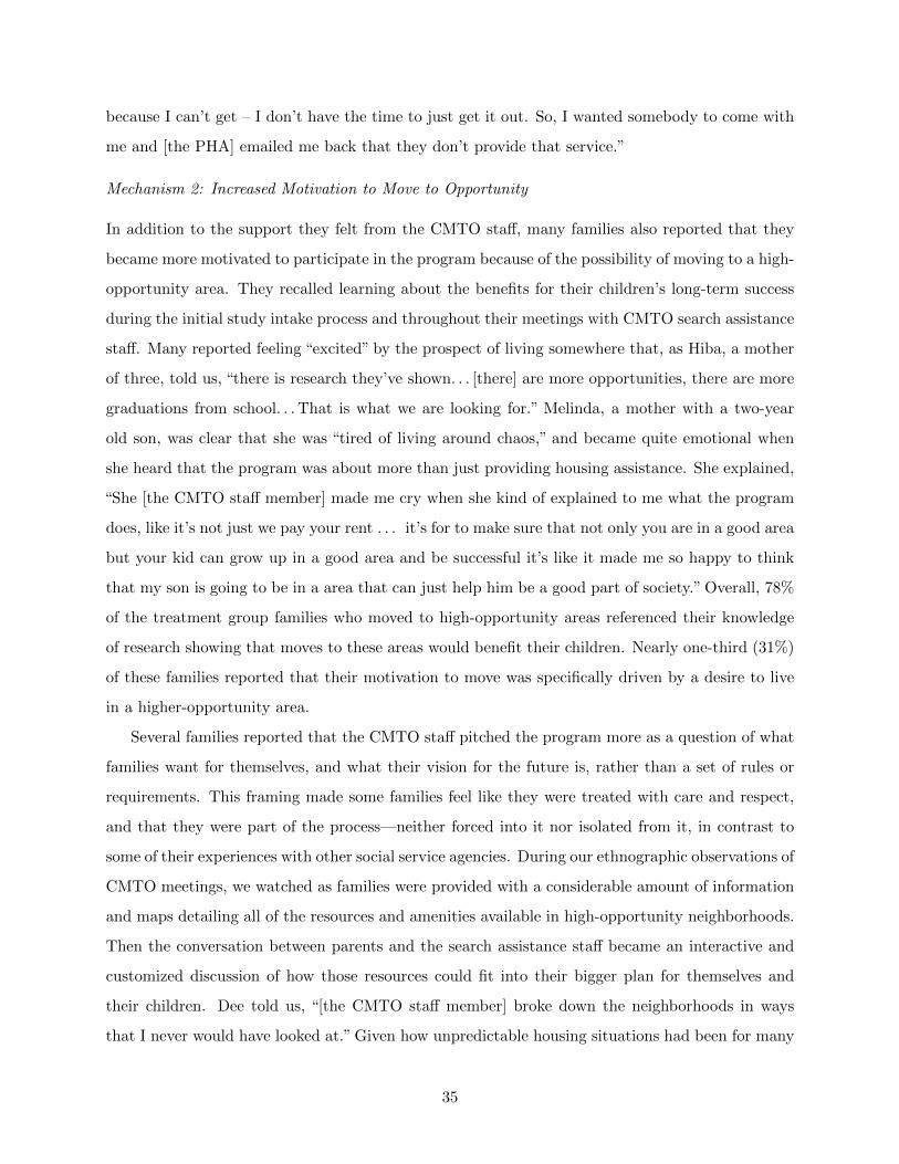
because I can’t get – I don’t have the time to just get it out. So, I wanted somebody to come with

me and [the PHA] emailed me back that they don’t provide that service.”

Mechanism 2: Increased Motivation to Move to Opportunity

In addition to the support they felt from the CMTO staff, many families also reported that they

became more motivated to participate in the program because of the possibility of moving to a high-

opportunity area. They recalled learning about the benefits for their children’s long-term success

during the initial study intake process and throughout their meetings with CMTO search assistance

staff. Many reported feeling “excited” by the prospect of living somewhere that, as Hiba, a mother

of three, told us, “there is research they’ve shown. . . [there] are more opportunities, there are more

graduations from school. . . That is what we are looking for.” Melinda, a mother with a two-year

old son, was clear that she was “tired of living around chaos,” and became quite emotional when

she heard that the program was about more than just providing housing assistance. She explained,

“She [the CMTO staff member] made me cry when she kind of explained to me what the program

does, like it’s not just we pay your rent . . . it’s for to make sure that not only you are in a good area

but your kid can grow up in a good area and be successful it’s like it made me so happy to think

that my son is going to be in a area that can just help him be a good part of society.” Overall, 78%

of the treatment group families who moved to high-opportunity areas referenced their knowledge

of research showing that moves to these areas would benefit their children. Nearly one-third (31%)

of these families reported that their motivation to move was specifically driven by a desire to live

in a higher-opportunity area.

Several families reported that the CMTO staff pitched the program more as a question of what

families want for themselves, and what their vision for the future is, rather than a set of rules or

requirements. This framing made some families feel like they were treated with care and respect,

and that they were part of the process—neither forced into it nor isolated from it, in contrast to

some of their experiences with other social service agencies. During our ethnographic observations of

CMTO meetings, we watched as families were provided with a considerable amount of information

and maps detailing all of the resources and amenities available in high-opportunity neighborhoods.

Then the conversation between parents and the search assistance staff became an interactive and

customized discussion of how those resources could fit into their bigger plan for themselves and

their children. Dee told us, “[the CMTO staff member] broke down the neighborhoods in ways

that I never would have looked at.” Given how unpredictable housing situations had been for many

35

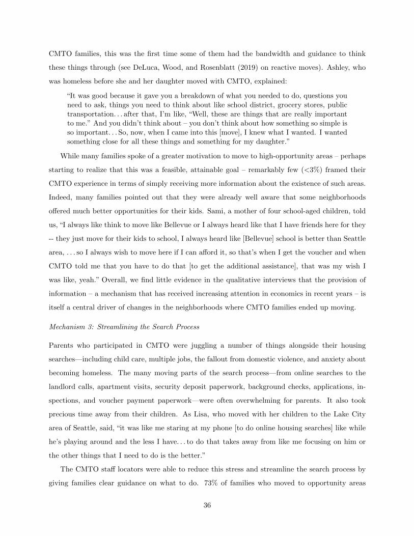
CMTO families, this was the first time some of them had the bandwidth and guidance to think

these things through (see DeLuca, Wood, and Rosenblatt (2019) on reactive moves). Ashley, who

was homeless before she and her daughter moved with CMTO, explained:

“It was good because it gave you a breakdown of what you needed to do, questions youneed to ask, things you need to think about like school district, grocery stores, publictransportation. . . after that, I’m like, “Well, these are things that are really importantto me.” And you didn’t think about – you don’t think about how something so simple isso important. . . So, now, when I came into this [move], I knew what I wanted. I wantedsomething close for all these things and something for my daughter.”

While many families spoke of a greater motivation to move to high-opportunity areas – perhaps

starting to realize that this was a feasible, attainable goal – remarkably few (<3%) framed their

CMTO experience in terms of simply receiving more information about the existence of such areas.

Indeed, many families pointed out that they were already well aware that some neighborhoods

offered much better opportunities for their kids. Sami, a mother of four school-aged children, told

us, “I always like think to move like Bellevue or I always heard like that I have friends here for they

-- they just move for their kids to school, I always heard like [Bellevue] school is better than Seattle

area, . . . so I always wish to move here if I can afford it, so that’s when I get the voucher and when

CMTO told me that you have to do that [to get the additional assistance], that was my wish I

was like, yeah.” Overall, we find little evidence in the qualitative interviews that the provision of

information – a mechanism that has received increasing attention in economics in recent years – is

itself a central driver of changes in the neighborhoods where CMTO families ended up moving.

Mechanism 3: Streamlining the Search Process

Parents who participated in CMTO were juggling a number of things alongside their housing

searches—including child care, multiple jobs, the fallout from domestic violence, and anxiety about

becoming homeless. The many moving parts of the search process—from online searches to the

landlord calls, apartment visits, security deposit paperwork, background checks, applications, in-

spections, and voucher payment paperwork—were often overwhelming for parents. It also took

precious time away from their children. As Lisa, who moved with her children to the Lake City

area of Seattle, said, “it was like me staring at my phone [to do online housing searches] like while

he’s playing around and the less I have. . . to do that takes away from like me focusing on him or

the other things that I need to do is the better.”

The CMTO staff locators were able to reduce this stress and streamline the search process by

giving families clear guidance on what to do. 73% of families who moved to opportunity areas

36

mention that their housing search and lease-up processes were made simpler, quicker and less

overwhelming by the assistance they received from CMTO staff. Some families also referred to a

“plan” that they worked on with the CMTO search assistance staff. Others mentioned doing their

“homework” to search for places, practice their landlord phone call script, and write down their

attempts to find housing in their “search log.”

The program also reduced the tax of fruitless and demoralizing housing searches by directly

providing listings of rental units that were owned by landlords and property management companies

with whom the CMTO staff had built relationships. The CMTO staff built trust with property

owners and managers and increased the information these housing providers have about families,

thus reducing the influence of “Section 8” stereotypes. Melinda explained how the list of referrals

she received from her housing locator made it easier to find the place she moved into:

“She gave me a list of apartments that CMTO worked with and I just based my searchoff of that list, so, cuz I was nervous about my credit and I just didn’t wanna go througha whole bunch of denials if, you know, they’re familiar with this program, then it’ll beeasier for me to get in. . . I don’t think I would’ve tried out here honestly without themgiving me like the areas that they feel like are more opportunities.”

Mechanism 4: Landlord Brokering

The CMTO staff played a key role in facilitating relationships between prospective tenants and

landlords, both in preparing the tenants before they met landlords and in participating in con-

versations with landlords themselves. 61% of the families interviewed reported that CMTO staff

helped negotiate directly with landlords on their behalf during some part of the process.

One key element of housing search preparation was the creation of a “rental resume,” a docu-

ment that families could use to present themselves to landlords. The essays helped families explain

the circumstances surrounding barriers to housing, like poor credit histories, evictions or unem-

ployment. Some families felt empowered by creating their rental resumes to help move beyond past

barriers and achieve their hoped-for future through opportunity moves. The resumes also allowed

the housing search assistance staff to better describe families in their conversations with prospective

landlords.

Nicole, who moved with her 5-year-old son, described in detail how the rental resume seemed to

make a big difference to the leasing company she ended up working with, despite her spotty credit

history:

“Some landlords, you know, your credit could get denied like here like mine did andthey could like you based on that [rental resume] and then, [ask] you [for] a higher

37

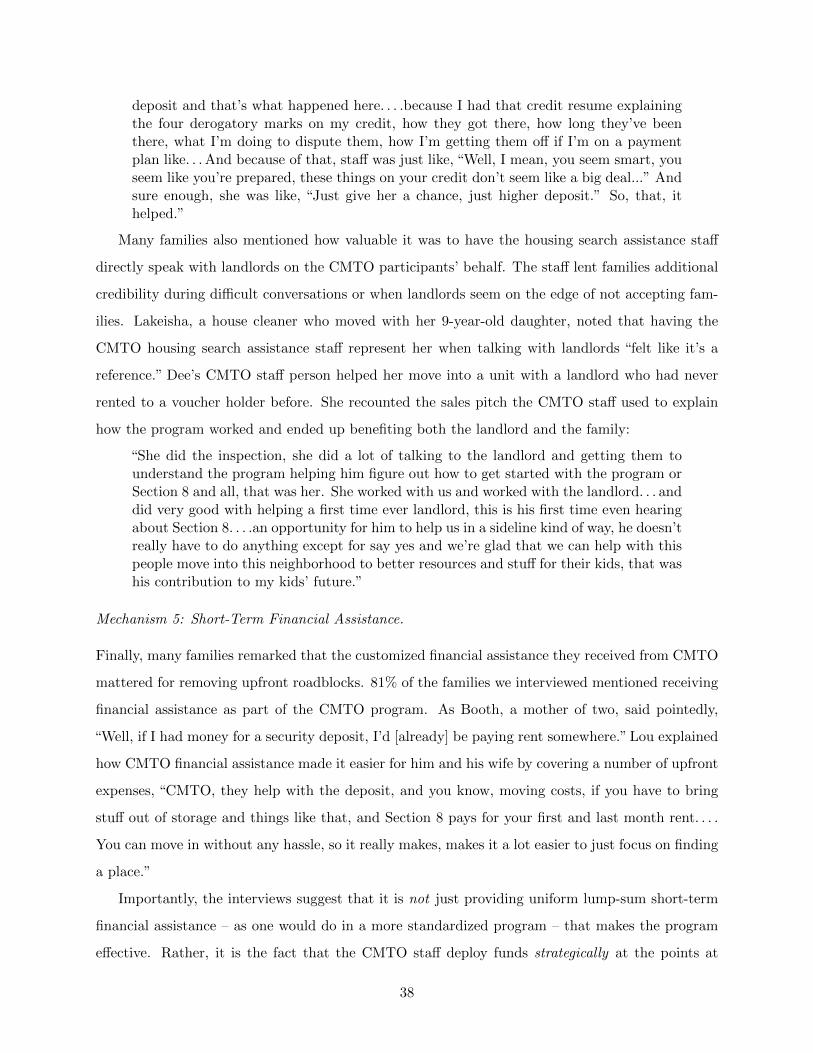
deposit and that’s what happened here. . . .because I had that credit resume explainingthe four derogatory marks on my credit, how they got there, how long they’ve beenthere, what I’m doing to dispute them, how I’m getting them off if I’m on a paymentplan like. . . And because of that, staff was just like, “Well, I mean, you seem smart, youseem like you’re prepared, these things on your credit don’t seem like a big deal...” Andsure enough, she was like, “Just give her a chance, just higher deposit.” So, that, ithelped.”

Many families also mentioned how valuable it was to have the housing search assistance staff

directly speak with landlords on the CMTO participants’ behalf. The staff lent families additional

credibility during difficult conversations or when landlords seem on the edge of not accepting fam-

ilies. Lakeisha, a house cleaner who moved with her 9-year-old daughter, noted that having the

CMTO housing search assistance staff represent her when talking with landlords “felt like it’s a

reference.” Dee’s CMTO staff person helped her move into a unit with a landlord who had never

rented to a voucher holder before. She recounted the sales pitch the CMTO staff used to explain

how the program worked and ended up benefiting both the landlord and the family:

“She did the inspection, she did a lot of talking to the landlord and getting them tounderstand the program helping him figure out how to get started with the program orSection 8 and all, that was her. She worked with us and worked with the landlord. . . anddid very good with helping a first time ever landlord, this is his first time even hearingabout Section 8. . . .an opportunity for him to help us in a sideline kind of way, he doesn’treally have to do anything except for say yes and we’re glad that we can help with thispeople move into this neighborhood to better resources and stuff for their kids, that washis contribution to my kids’ future.”

Mechanism 5: Short-Term Financial Assistance.

Finally, many families remarked that the customized financial assistance they received from CMTO

mattered for removing upfront roadblocks. 81% of the families we interviewed mentioned receiving

financial assistance as part of the CMTO program. As Booth, a mother of two, said pointedly,

“Well, if I had money for a security deposit, I’d [already] be paying rent somewhere.” Lou explained

how CMTO financial assistance made it easier for him and his wife by covering a number of upfront

expenses, “CMTO, they help with the deposit, and you know, moving costs, if you have to bring

stuff out of storage and things like that, and Section 8 pays for your first and last month rent. . . .

You can move in without any hassle, so it really makes, makes it a lot easier to just focus on finding

a place.”

Importantly, the interviews suggest that it is not just providing uniform lump-sum short-term

financial assistance – as one would do in a more standardized program – that makes the program

effective. Rather, it is the fact that the CMTO staff deploy funds strategically at the points at

38

which it is easiest to lose hope and lose landlords. Such timely financial assistance included paying

rental application fees, paying “holding” fees so families don’t lose their units while applications are

being processed, clearing up old utility bills or paying for new ones, and providing more generous

security deposits for families with a past eviction or poor credit record. For example, Stive, a father

of two, explained:

“She [the CMTO search assistance staff member] paid security deposit, I gave her theaccess to my personal page in the [website] of the home, of this apartment complex.And yes, it was really helpful it was quick, because I was so afraid [of losing the place]when I find it out that I have to make a decision about [taking the apartment], andin the same time I have to pay security deposits and a couple fees [when] I don’t haveresources.”

VI.C Customization of Services to Families’ Needs

The CMTO staff facilitated lease-ups in opportunity areas by combining several of the five ap-

proaches discussed above, depending upon each family’s specific needs. For example, the emotional

and psychological support keeps families connected to the program and optimistic about the end

result of the process, which is necessary to motivate their individual housing search efforts, and

to get them to the point where the CMTO staff can do the work of connecting with landlords in

opportunity areas and completing the lease-up process. The customization of CMTO services –

with nonprofit staff being able to flexibly respond to each family’s specific situation and needs –

appears to be crucial to its success. For instance, Jennifer, a mother of four, noted that the CMTO

staff “understood the situation that I was in” and helped her accordingly.

Although many families mentioned several of the five mechanisms described above in their

interviews, the intensity with which they used each component of the CMTO program varied

greatly. This is borne out by data on service utilization from our case management system, which

tracked the duration and nature of each of the contacts between CMTO staff and families. We

report statistics on rates of service utilization in Appendix Table 9a. CMTO treatment group

families who moved to a high-opportunity area received 7.05 hours of staff time on average, but

there was substantial heterogeneity in the utilization of these services, with an interquartile range of

about 4 hours to 9 hours. Similarly mean financial assistance for treatment group families leasing

up in opportunity areas was $1,983 dollars, with an interquartile range of $958 to $3009. 47%

of these families found the unit they moved into through a direct referral to a landlord found by

CMTO staff, but 53% identified the units they moved into on their own. Different families also

used different subsets of these services: for instance, the correlation between the number of hours

39

of staff time used and the amount of financial assistance used is 0.19 (Appendix Table 9d).

When we talked to families in the control group, we virtually never heard them discuss receiv-

ing this kind of customized assistance, although several mentioned that they wished they had it.

Christina, the mother of a six-year-old daughter, described how much she struggled to find housing

herself:

“I went through [local housing provider agency] to see if they could help me find anapartment. Nobody really helps you find an apartment. They just tell you that theylike can help you get into it or they tell you that they can help you find one but theydon’t end up doing that cuz they have a lot of people that they’re working with. . . Ifound this place [on my own]. I have sent emails back and forth begging to get inhere. . . my application was sitting downstairs approved for like two days while I’m stillin cars and outside with my daughter trying to figure it out. I could’ve been in here atan empty apartment at least with warmth. So, I ended up getting accepted for here.[Local non-profit housing provider] ended up paying for the move in fees and stuff likethat which was a blessing but I feel like maybe if they could be more personal withtheir clients that they’re accepting and taking on that I feel like that would help withthe homeless situation a lot.”

In sum, the CMTO program appears to have had large impacts through a combination of

mechanisms that addressed each family’s specific challenges, while also negotiating with landlords

who might not otherwise rent to a family with a voucher. In light of the findings on scarcity of

bandwidth in Section VI.A, one way to summarize the program’s mechanism is that it provides

emotional and other support that enables families to optimize over neighborhood choice as posited

in traditional economic models, thereby allowing them to realize their inherent preference for higher

opportunity areas (Harvey et al. 2019; DeLuca and Jang 2020). We believe that the fact that the

intervention cannot be easily codified into a standardized set of protocols applied to all families

underlies its efficacy. The customization of services may also have been beneficial in reducing

program costs, as families who did not need certain components of the services (e.g., help with

landlords or security deposit assistance) took up less resources from those parts of the program.

The general lesson may be that having a highly motivated case worker support each family in

overcoming the barriers they face can help them make much more effective use of housing assistance

programs (and perhaps other public programs more generally).

VII Alternative Policies to Increase Moves to Opportunity

In this section, we compare the impacts of the CMTO program to other, more standardized policies

that aim to help families move to higher opportunity areas: financial incentives and information

provision. We estimate the effects of financial incentives by analyzing the impacts of reforms

40

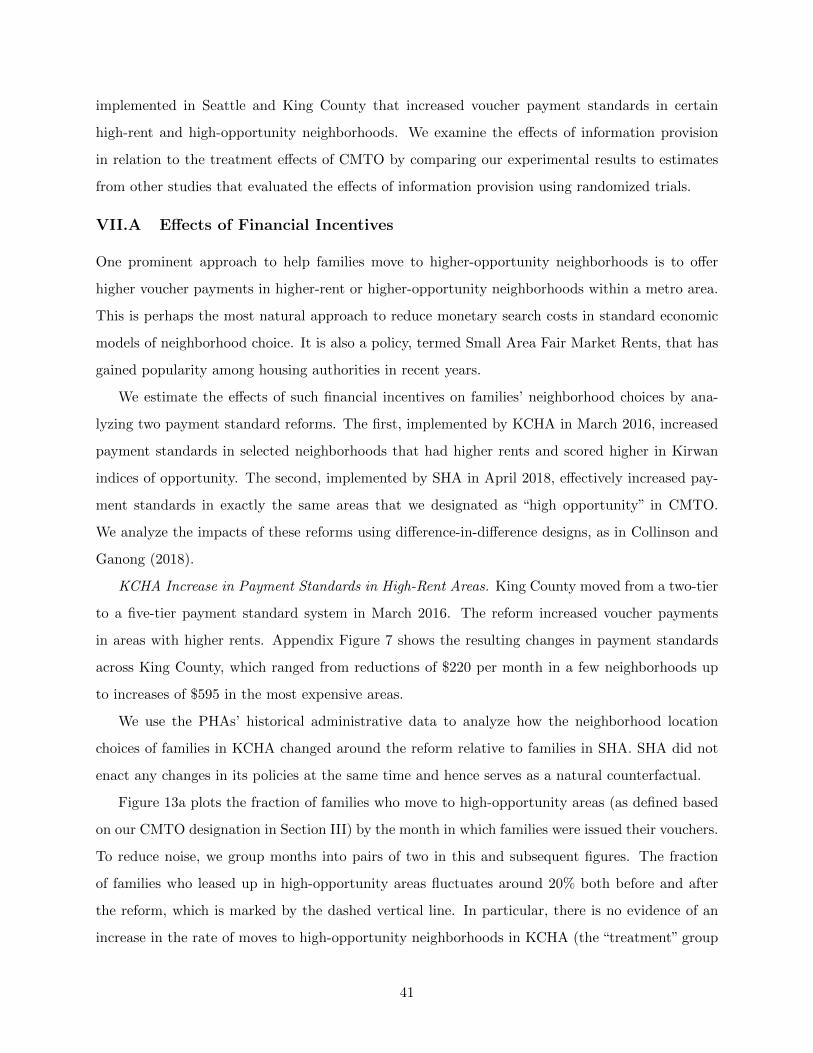
implemented in Seattle and King County that increased voucher payment standards in certain

high-rent and high-opportunity neighborhoods. We examine the effects of information provision

in relation to the treatment effects of CMTO by comparing our experimental results to estimates

from other studies that evaluated the effects of information provision using randomized trials.

VII.A Effects of Financial Incentives

One prominent approach to help families move to higher-opportunity neighborhoods is to offer

higher voucher payments in higher-rent or higher-opportunity neighborhoods within a metro area.

This is perhaps the most natural approach to reduce monetary search costs in standard economic

models of neighborhood choice. It is also a policy, termed Small Area Fair Market Rents, that has

gained popularity among housing authorities in recent years.

We estimate the effects of such financial incentives on families’ neighborhood choices by ana-

lyzing two payment standard reforms. The first, implemented by KCHA in March 2016, increased

payment standards in selected neighborhoods that had higher rents and scored higher in Kirwan

indices of opportunity. The second, implemented by SHA in April 2018, effectively increased pay-

ment standards in exactly the same areas that we designated as “high opportunity” in CMTO.

We analyze the impacts of these reforms using difference-in-difference designs, as in Collinson and

Ganong (2018).

KCHA Increase in Payment Standards in High-Rent Areas. King County moved from a two-tier

to a five-tier payment standard system in March 2016. The reform increased voucher payments

in areas with higher rents. Appendix Figure 7 shows the resulting changes in payment standards

across King County, which ranged from reductions of $220 per month in a few neighborhoods up

to increases of $595 in the most expensive areas.

We use the PHAs’ historical administrative data to analyze how the neighborhood location

choices of families in KCHA changed around the reform relative to families in SHA. SHA did not

enact any changes in its policies at the same time and hence serves as a natural counterfactual.

Figure 13a plots the fraction of families who move to high-opportunity areas (as defined based

on our CMTO designation in Section III) by the month in which families were issued their vouchers.

To reduce noise, we group months into pairs of two in this and subsequent figures. The fraction

of families who leased up in high-opportunity areas fluctuates around 20% both before and after

the reform, which is marked by the dashed vertical line. In particular, there is no evidence of an

increase in the rate of moves to high-opportunity neighborhoods in KCHA (the “treatment” group

41

for the purposes of this quasi-experiment) relative to SHA (the “control” group).

Under the identification assumption that trends in KCHA and SHA would have remained similar

absent the reform, we can estimate the causal effect of the KCHA payment standard reform on

the rate of moves to high-opportunity areas using a standard difference-in-difference regression

specification. We compare the rate of moves to high-opportunity areas in KCHA and SHA in the

eight months before vs. after the policy change by running OLS regressions of the form:

yi = α+ β1KCHAi + β2Posti + β3KCHAi × Posti + εi, (2)

where yi is an indicator for moving to a high-opportunity neighborhood, KCHAi is an indicator

for receiving a voucher from KCHA (rather than SHA), and Posti is an indicator for being issued

a voucher in or after March 2016. We estimate that the causal effect of the reform on the rate of

moves to high-opportunity areas is a statistically insignificant β3 =-3.6% (s.e. = 5.8), as shown in

Column 1 of Table 4. Controlling for family size and other covariates does not affect this estimate

significantly (Column 2).45 Hence, the KCHA reform increased the rate of opportunity moves by

at most 7.7pp at the top of the 95% confidence interval – substantially smaller than the CMTO

treatment effect of 37.9%, shown by the dashed line in Figure 13a as a reference. Indeed, only

17.5% of KCHA families with children moved to high-opportunity areas in the eight months after

the payment standard increase, far below the 53.0% rate achieved through the CMTO program in

King County.

Our analysis of the KCHA reform shows that raising payment standards in more expensive

neighborhoods – as is typically done in SAFMR policies – does not necessarily induce families to

move to higher-opportunity areas.46 One interpretation of this result is that financial incentives

have smaller impacts on neighborhood choice than the customized services offered through CMTO.

An alternative interpretation is that incentivizing families to move to more expensive neighborhoods

45. Analogous DD specifications using median rents as the dependent variable suggest that the SAFMR reforminduced families to move to more expensive areas (Columns 3 and 4 of Table 4), consistent with Collinson andGanong (2018), although the estimates are somewhat imprecise and hence not statistically significant.

46. In contrast with this finding, Collinson and Ganong (2018) find that SAFMRs induced moves to higher-qualityneighborhoods in Dallas, where quality is defined as an index of tract-level poverty rate, test scores, unemploymentrate, the share of children with single mothers, and the violent crime rate. By contrast, we find that SAFMRs in KingCounty had no impact on either an index of neighborhood quality similar to that used by Collinson and Ganong orthe Opportunity Atlas measures of upward mobility. One explanation for the different results is that the correlationbetween rents and upward mobility is 0.56 in Dallas, significantly higher than the 0.18 correlation in King County.The tighter link between rents and opportunity in Dallas might increase the impacts of SAFMRs on opportunitymoves there. That said, Collinson and Ganong kindly replicated their analysis using the Opportunity Atlas measureof upward mobility and found an impact on the mean predicted rank of children with parents at the 25th percentileof 0.86 percentiles. Although this is a significant gain, it is still considerably smaller than the impact of CMTO,supporting the view that financial incentives have much smaller effects than customized mobility services.

42

does not induce moves to opportunity because rents are not very highly correlated with upward

mobility in King County (Figure 1b). To distinguish between these explanations, we now turn to

a second quasi-experiment.

SHA Increase in Payment Standards in High-Opportunity Areas. In March 2018, SHA intro-

duced a Family Access Supplement (FAS) that effectively increased payment standards in areas

that were designated as “high opportunity” in the CMTO study. If a family moved to an opportu-

nity area and the unit rent exceeded the voucher payment standard by an amount that would cause

the household to pay more than 40% of their income, the FAS paid for the unit’s rent minus 40%

of the family’s income (subject to a maximum, which was $400 for 2 bedroom units). For families

who moved to an opportunity area, this additional rental support amounted to $144 per month on

average.

The FAS was initiated at the same time as a pilot phase of the CMTO intervention prior to the

CMTO experiment. It continued throughout the pilot and the experiment, effectively providing

families in the control group higher payments to move to high-opportunity areas than they would

have received had they gotten their vouchers before March 2018. The FAS was restricted to families

with at least one child under 18. We therefore estimate the impact of the FAS by comparing families

with children to families without children in SHA.47

Figure 13b plots the fraction of families moving to high-opportunity areas before and after the

introduction of the FAS (shown by the dashed line) for households with vs. without children.

During the CMTO pilot phase (shown in the shaded region), all families with children received

CMTO services. The fraction of families moving to high-opportunity areas trended similarly prior

to the CMTO pilot and the FAS payment standard reform. During the pilot, the rate of moves to

opportunity for those with children spiked up to 80%, while the rate of such moves for the those

without children (who were untreated) remained steady. After the pilot, the rate of opportunity

moves (based on data for the CMTO control group) fell precipitously for families with children.

Under the identification assumption that the rate of opportunity moves for families with vs.

without children would have remained similar after March 2018 in the absence of the FAS, we can

infer that the SHA reform caused a small increase in the rate of moves to high-opportunity ar-

eas. Using a standard difference-in-differences specification comparing the rate of high-opportunity

moves among families with vs. without children in SHA in the six months before March 2018 vs.

47. We do not use KCHA as a counterfactual here because KCHA itself was implementing its CMTO pilot at thesame time that SHA introduced the FAS.

43

the six months after May 2018 (after the CMTO pilot ended, using only families in the CMTO

control), we estimate that the FAS increased the rate of opportunity moves by 13.8 pp (s.e. = 5.1),

as shown in Column 5 of Table 4. This is roughly one-third the size of the CMTO treatment effect.

The FAS has a recurring monthly cost of $144 on average for families who move to high-

opportunity areas, which amounts to $12,100 over 7 years (the average period for which families

use their vouchers). This is substantially larger than the cost of CMTO mobility services, which

are about $5,010 per family that moved to a high-opportunity area. We therefore conclude that

financial incentives have significantly smaller impacts per dollar of expenditure than customized

mobility services even when targeted directly to high-opportunity areas.

Although these findings show that standardized financial incentives by themselves have lim-

ited impacts on the fraction of families who move to opportunity, there could potentially be an

interaction effect whereby the mobility services in CMTO were more effective because the housing

authorities were offering enhanced payment standards that enabled families to move to more ex-

pensive, higher-opportunity neighborhoods. While we do not have direct experimental evidence on

what the treatment effects of CMTO would be in the absence of such tiered payment standards, we

find that 34% of the treatment group families who moved to high-opportunity areas leased up units

that they would have been able to afford even in the absence of the enhanced payment standards

described above (i.e., in the absence of the FAS supplement in SHA and under the pre-March-2016

two-tier system in KCHA). This finding suggests that CMTO mobility services would have substan-

tial impacts even in the absence of differential payment standards across neighborhoods, though

further work is necessary to quantify how effective the program would be in such settings.48

VII.B Effects of Information Provision

Another alternative to customized housing search assistance is to provide information in a more

standardized manner. Bergman, Chan, and Kapor (2019) randomized the provision of information

to families about the quality of schools associated with rental units on GoSection8.com, a housing

search platform widely used by voucher holders. They find small positive impacts of this low-cost

intervention on the fraction of families who move to areas with better schools, with treatment

effects considerably smaller than those induced by CMTO. Families who received the information

treatment moved to neighborhoods with schools scoring 0.1 standard deviations (SD) better on

48. This 34% figure should be interpreted as a lower bound on the fraction of families one would be observe movingto a high-opportunity area with the CMTO treatment in the absence of the higher payment standards since manyfamilies would presumably still move to high-opportunity areas, but choose less expensive units than the ones theychose given current policies.

44

state tests on average. By contrast, the CMTO intervention induced treatment group families to

move to neighborhoods with schools scoring 0.5 SDs higher on state tests. Moreover, using data

from the Opportunity Atlas, Bergman et al. estimate that the effect of the additional information

on predicted household income rank is 16% as large as the CMTO impact on upward mobility

shown in Figure 4d.

Schwartz, Mihaly, and Gala (2017) report results from a randomized trial in Chicago in which

families receiving housing vouchers were given $500 of financial assistance and light-touch mobility

counseling services to move to a high-opportunity area (defined based on a composite index of

poverty rates, job access, and other characteristics). The counseling services offered in the Chicago

trial were largely informational and “client-led” as opposed to the more intensive counselor-led

services offered in CMTO. They find that these treatments had no impact on the rate of high-

opportunity moves: less than 12% of families moved to high-opportunity neighborhoods even with

these incentives and supports.

Supplementary evidence from our own data further supports the view that standardized infor-

mation provision is unlikely to be adequate to induce moves to opportunity. The CMTO treatment

increased the fraction of families living in high-opportunity Census tracts substantially (48 pp)

even among families who lived in high-opportunity areas at baseline (Table 2). Since these families

presumably were familiar with these neighborhoods to begin with, this finding weighs against the

view that a lack of information is the central reason families do not move to opportunity. Further-

more, 72% of families report that they feel “good” or “very good” about moving to an opportunity

neighborhood in the baseline survey, before the CMTO intervention began, again suggesting that

they do not lack information about such areas.

Together, the results in this section suggest that the mechanisms through which the CMTO

intervention works are not simply the provision of financial incentives or information about high-

opportunity areas. These findings are consistent with the qualitative evidence discussed above, and

suggest that customized support in the search process and help in engaging landlords are likely to

be pivotal elements in the program’s success.

VIII Conclusion

Low-income families tend to live in neighborhoods that offer limited prospects for upward income

mobility, amplifying the persistence of poverty across generations. This paper has shown that

this pattern of segregation is not driven by deep-rooted preferences among tenants or landlords.

45

Rather, low-income families live in such areas primarily because of barriers that prevent them from

moving to higher-opportunity neighborhoods – barriers that can be overcome through short-term

assistance in the housing search process. These findings challenge canonical economic models of

neighborhood choice in which residential sorting patterns are determined primarily by families’

preferences and call for greater modeling of the underlying structure of search costs. The findings

also advance canonical sociological models of neighborhood choice and residential mobility, in which

barriers such as discrimination have received greater emphasis (D. S. Massey and N. A. Denton

1993; Yinger 1995; South and Crowder 1997), because they reveal that some of the barriers families

face can be overcome through a modest amount of assistance in the housing search process.49

More broadly, our findings suggest that the growing economic segregation of American cities

(Reardon and Bischoff 2011) is not an inevitable consequence of preferences (either among tenants

or landlords), but rather a trend that can be addressed through modest changes in public policies.

In particular, redesigning rental assistance programs to provide customized search assistance in

addition to existing financial support could reduce segregation and thereby increase upward mobility

significantly. Such programs could have little net cost to taxpayers, as the costs of the up-front

services could be offset by the increased tax revenue paid by children who earn more when they

grow up.

Going forward, it would be useful to replicate the CMTO program implemented in Seattle and

King County in other cities to understand whether the program can be scaled nationally with the

same level of effectiveness. In parallel, recognizing that not all families can move to opportunity,

we also hope to identify place-based investments that can improve outcomes for residents of lower-

opportunity areas.

49. These conclusions are in line with Krysan and Crowder’s (2017) discussion of policies to break the cycle ofsegregation.

46

References

Acevedo-Garcia, Dolores, Nancy McArdle, Erin F. Hardy, Unda Ioana Crisan, Bethany Romano,

David Norris, Mikyung Baek, and Jason Reece. 2014.“The Child Opportunity Index: Improving

Collaboration Between Community Development And Public Health.”PMID: 25367989, Health

Affairs 33 (11): 1948–1957. doi:10.1377/hlthaff.2014.0679. eprint: https://doi.org/10.

1377/hlthaff.2014.0679. https://doi.org/10.1377/hlthaff.2014.0679.

Anderson, Elijah. 1990. Streetwise: Race, class, and change in an urban community. University of

Chicago Press.

Andrews, Isaiah, Toru Kitagawa, and Adam McCloskey. 2019. Inference on Winners. NBER Work-

ing Paper 25456. National Bureau of Economic Research, Inc, January. https://www.nber.

org/papers/w25456.

Basolo, Victoria, and Anaid Yerena. 2017. “Residential mobility of low-income, subsidized house-

holds: a synthesis of explanatory frameworks.” Housing Studies 32 (6): 841–862.

Bayer, Patrick, Fernando Ferreira, and Robert McMillan. 2007.“A Unified Framework for Measuring

Preferences for Schools and Neighborhoods.” Journal of Political Economy 115 (4): 588–638.

Becker, Howard S, Blanche Geer, Everett C Hughes, and Anselm L Strauss. 1961. Boys in white:

Student culture in medical school. New Brunswick. NJ: Transaction Books.

Bergman, Peter, Eric Chan, and Adam Kapor. 2019. “Housing Search Frictions: Evidence from

Detailed Search Data and a Field Experiment.”

Boyd, Melody, and Stefanie DeLuca. 2017.“Fieldwork with in-depth interviews: How to get strangers

in the city to tell you their stories.” Methods in social epidemiology: 239–253.

Burawoy, Michael. 1979. Manufacturing consent. Changes in the labor process under monopoly

capitalism. Chicago, University of Chicago Press.

Charles, Camille Zubrinsky. 2003. “The Dynamics of Racial Residential Segregation.” Annual Re-

view of Sociology 29:167–207.

. 2005.“Can we live together? Racial preferences and neighborhood outcomes.”The geography

of opportunity: Race and housing choice in metropolitan America 45.

Chetty, Raj, John N Friedman, Nathaniel Hendren, Maggie R Jones, and Sonya R Porter. 2018. The

Opportunity Atlas: Mapping the Childhood Roots of Social Mobility. Working Paper, Working

Paper Series 25147. National Bureau of Economic Research, October.

Chetty, Raj, and Nathaniel Hendren. 2018a. “The Impacts of Neighborhoods on Intergenerational

Mobility I: Childhood Exposure Effects.” The Quarterly Journal of Economics 133 (3): 1107–

1162.

47

Chetty, Raj, and Nathaniel Hendren. 2018b. “The Impacts of Neighborhoods on Intergenerational

Mobility II: County-Level Estimates.”The Quarterly Journal of Economics 133 (3): 1163–1228.

Chetty, Raj, Nathaniel Hendren, and Lawrence F. Katz. 2016. “The Effects of Exposure to Better

Neighborhoods on Children: New Evidence from the Moving to Opportunity Experiment.”

American Economic Review 106 (4): 855–902.

Chetty, Raj, Nathaniel Hendren, Patrick Kline, and Emanuel Saez. 2013. “The Economic Impacts

of Tax Expenditures: Evidence from Spatial Variation Across the U.S.” SOI Whitepaper.

Chyn, Eric. 2018. “Moved to opportunity: The long-run effects of public housing demolition on

children.” American Economic Review 108 (10): 3028–56.

Clark, William AV. 2008. “Reexamining the moving to opportunity study and its contribution to

changing the distribution of poverty and ethnic concentration.” Demography 45 (3): 515–535.

Clark, William AV, and Valerie Ledwith. 2006. “Mobility, housing stress, and neighborhood con-

texts: evidence from Los Angeles.” Environment and Planning A 38 (6): 1077–1093.

Collinson, Robert, Ingrid Gould Ellen, and Jens Ludwig. 2015. “Low-income housing policy.” In

Economics of Means-Tested Transfer Programs in the United States, 2:59–126. University of

Chicago Press.

Collinson, Robert, and Peter Ganong. 2018. “How Do Changes in Housing Voucher Design Affect

Rent and Neighborhood Quality?” American Economic Journal: Economic Policy 10 (2): 62–

89.

Cunningham, Mary K, and Susan J Popkin. 2002. CHAC Mobility Counseling Assessment. Final

Report. Technical report. Washington, DC: The Urban Institute.

Darrah, Jennifer, and Stefanie DeLuca. 2014. “”Living here has changed my whole perspective”:

How escaping inner-city poverty shapes neighborhood and housing choice.” Journal of Policy

Analysis and Management 33 (2): 350–384.

Davis, Morris A, Jesse Gregory, and Daniel A Hartley. 2018. “The Long Run Effects of Low Income

Housing on Neighborhood Composition.”

Davis, Morris A, Jesse Gregory, Daniel A Hartley, and Kegon Tan. 2017. “Neighborhood choices,

neighborhood effects and housing vouchers.” FRB of Chicago Working Paper No. WP-2017-2.

DeLuca, Stefanie, Susan Clampet-Lundquist, and Kathryn Edin. 2016. Coming of Age in the Other

America. Russell Sage Foundation.

DeLuca, Stefanie, and Christine Jang. Forthcoming 2020. “Decision-making in the Housing and

Neighborhood Selection Process.” City and Community.

48

DeLuca, Stefanie, and James E Rosenbaum. 2003. “If low-income blacks are given a chance to live

in white neighborhoods, will they stay? Examining mobility patterns in a quasi-experimental

program with administrative data.” Housing Policy Debate 14 (3): 305–345.

DeLuca, Stefanie, and Peter Rosenblatt. 2017. “Walking away from the wire: Housing mobility and

neighborhood opportunity in Baltimore.” Housing Policy Debate 27 (4): 519–546.

DeLuca, Stefanie, Holly Wood, and Peter Rosenblatt. 2019. “Why poor families move (and where

they go): Reactive mobility and residential decisions.” City & Community 18 (2): 556–593.

Desmond, Matthew, and Tracey Shollenberger. 2015. “Forced displacement from rental housing:

Prevalence and neighborhood consequences.” Demography 52 (5): 1751–1772.

Deutscher, Nathan. 2018.“Place, Jobs, Peers and the Importance of the Teenage Years: Exposure Ef-

fects and Intergenerational Mobility.” Australian National University, unpublished manuscript.

Edin, Kathryn, and Laura Lein. 1997. Making ends meet: How single mothers survive welfare and

low-wage work. Russell Sage Foundation.

Emerson, Michael O, Karen J Chai, and George Yancey. 2001. “Does race matter in residential

segregation? Exploring the preferences of white Americans.” American Sociological Review:

922–935.

Fahle, Erin M, Benjamin R Shear, Demetra Kalogrides, S Reardon, Richard DiSalvo, and Andrew

D Ho. 2017. “Stanford education data archive.”

Faurschou, Ebbe. 2018. “Quasi-experimental evidence of neighbourhood exposure effects in Den-

mark.” PhD diss., University of Copenhagen.

Feins, Judith, Debra McInnis, and Susan J Popkin. 1997. Counseling in the moving to opportunity

demonstration program. Technical report. Department of Housing and Urban Development.

Galiani, Sebastian, Alvin Murphy, and Juan Pantano. 2015. “Estimating neighborhood choice mod-

els: Lessons from a housing assistance experiment.”American Economic Review 105 (11): 3385–

3415.

Garboden, Philip ME, Eva Rosen, Stefanie DeLuca, and Kathryn Edin. 2018. “Taking stock: What

drives landlord participation in the housing choice voucher program.” Housing Policy Debate

28 (6): 979–1003.

Harvey, Hope, Kelley Fong, Kathryn Edin, and Stefanie DeLuca. 2019. “Forever Homes and Tem-

porary Stops: Housing Search Logics and Residential Selection.” Social Forces.

49

HUD. 2016. Establishing a More Effective Fair Market Rent System; Using Small Area Fair Market

Rents in the Housing Choice Voucher Program Instead of the Current 50th Percentile FMRs,

November. https://www.federalregister.gov/documents/2016/11/16/2016-27114/

establishing-a-more-effective-fair-market-rent-system-using-small-area-fair-

market-rents-in-the.

Kain, John F, and John M Quigley. 1975. “Racial Discrimination in Urban Housing Markets.” In

Housing markets and racial discrimination: A microeconomic analysis, 56–91. NBER.

Kennan, John, and James R Walker. 2011. “The effect of expected income on individual migration

decisions.” Econometrica 79 (1): 211–251.

Kling, Jeffrey R., Jeffrey B. Liebman, and Lawrence F. Katz. 2007. “Experimental Analysis of

Neighborhood Effects.” Econometrica 75 (1): 83-119 75 (1): 83–119.

Krysan, Maria, and Michael DM Bader. 2009. “Racial blind spots: Black-white-Latino differences

in community knowledge.” Social Problems 56 (4): 677–701.

Krysan, Maria, and Kyle Crowder. 2017. Cycle of segregation: Social processes and residential

stratification. Russell Sage Foundation.

Laliberte, Jean-William P. 2018. “Long-term Contextual Effects in Education: Schools and Neigh-

borhoods.” University of Calgary, unpublished manuscript.

Lareau, Annette, and Kimberly Goyette. 2014. Choosing homes, choosing schools. Russell Sage

Foundation.

Liebow, Elliot. 1967. Tally’s corner: A study of Negro streetcorner men. Little, Brown.

Ludwig, Jens, Greg J. Duncan, Lisa A. Gennetian, Lawrence F. Katz, Ronald C. Kessler, Jeffrey R.

Kling, and Lisa Sanbonmatsu. 2012. “Neighborhood Effects on the Long-Term Well-Being of

Low-Income Adults.” Science 337 (6101): 1505-1510.

Massey, D., and N. Denton. 1987. “Trends in the Residential Segregation of Blacks, Hispanics, and

Asians: 1970-1980.” American Sociological Review 52 (6): 802–825. http://www.jstor.org/

stable/2095836.

Massey, Douglas S, and Nancy A Denton. 1993. American Apartheid: Segregation and the Making

of the Underclass [in English]. Cambridge, Mass.: Harvard University Press. isbn: 0674018206

9780674018204 0674018214 9780674018211.

Mazzara, Alicia, and Brian Knudsen. 2019. Where Families With Children Use Housing Vouchers,

January. https://www.cbpp.org/research/housing/where-families-with-children-

use-housing-vouchers.

Metzger, Molly W. 2014. “The reconcentration of poverty: Patterns of housing voucher use, 2000

to 2008.” Housing Policy Debate 24 (3): 544–567.

50

Mogstad, Magne, Joseph P Romano, Azeem M Shaikh, and Daniel Willhelm. 2020. Inference for

Ranks with Applications to Mobility Across Neighborhoods and Academic Achievement Across

Countries. Working Paper 2020-03. Stanford University, March. https://statistics.stanf

ord.edu/sites/g/files/sbiybj6031/f/2020-03.pdf.

Mullainathan, Sendhil, and Eldar Shafir. 2013. Scarcity: Why having too little means so much.

Macmillan.

Reardon, S, and Kendra Bischoff. 2011. “Income Inequality and Income Segregation.” American

Journal of Sociology 116 (4): 1092-1153.

Rinzler, Dan, Philip Tegeler, Mary K Cunningham, and Craig Pollack. 2015. “Leveraging the power

of place: Using pay for success to support housing mobility.” Federal Reserve Bank of San

Francisco Community Development Investment Center Working Paper 2015-04.

Roback, Jennifer. 1982. “Wages, rents, and the quality of life.” Journal of Political Economy 90 (6):

1257–1278.

Rosen, Sherwin. 1979. “Wage-Based Indices of Urban Quality of Life.” In Current Issues in Urban

Economics, edited by Peter Mieszkowski and Mahlon Straszheim, 74–104. Baltimore: Johns

Hopkins Univ. Press.

Sampson, Robert J. 2012. Great American City: Chicago and the Enduring Neighborhood Effect.

University of Chicago Press.

Sanbonmatsu, Lisa, Jens Ludwig, Lawrence F. Katz, Lisa A. Gennetian, Greg J. Duncan, Ronald C.

Kessler, Emma Adam, Thomas McDade, and Stacy Tessler Lindau. 2011. Moving to Oppor-

tunity for Fair Housing Demonstration Program: Final Impacts Evaluation. Washington, DC:

U.S. Department of Housing / Urban Development, Office of Policy Development / Research.

http://www.huduser.org/publications/pdf/MTOFHD_fullreport_v2.pdf.

Sard, Barbara, Mary K Cunningham, and Robert Greenstein. 2018. Helping Young Children Move

out of Poverty by Creating a New Type of Rental Voucher. US Partnership on Mobility from

Poverty.

Schelling, Thomas C. 1971. “Dynamic models of segregation.” Journal of Mathematical Sociology 1

(2): 143–186.

Schwartz, Heather L, Kata Mihaly, and Breann Gala. 2017. “Encouraging residential moves to

opportunity neighborhoods: An experiment testing incentives offered to housing voucher re-

cipients.” Housing Policy Debate 27 (2): 230–260.

Sharkey, Patrick. 2013. Stuck in Place: Urban Neighborhoods and the End of Progress Toward Racial

Equality. University of Chicago Press.

51

South, Scott J, and Kyle D Crowder. 1997. “Escaping distressed neighborhoods: Individual, com-

munity, and metropolitan influences.” American Journal of Sociology 102 (4): 1040–1084.

Turner, Margery Austin, Rob Santos, Diane K Levy, Doug Wissoker, Claudia Aranda, and Rob

Pitingolo. 2013. Housing discrimination against racial and ethnic minorities 2012: Executive

summary. U.S. Department of Housing, Urban Development, Policy Development, and Re-

search.

Wheaton, William C. 1990. “Vacancy, search, and prices in a housing market matching model.”

Journal of Political Economy 98 (6): 1270–1292.

Yinger, John. 1995. Closed doors, opportunities lost: The continuing costs of housing discrimination.

Russell Sage Foundation.

52

Online Appendix

A Algorithm for Constructing Opportunity Maps

We defined opportunity areas through a collaborative effort between the researchers and the staff ofthe Seattle and King County housing authorities. Here, we summarize the process through whichwe arrived at the final maps shown in Figure 2a.

Constructing Predictions of Upward Mobility by Census Tract. We begin from a preliminaryversion of the measures of upward mobility later published in the Opportunity Atlas (at the time theexperiment began, the final Opportunity Atlas estimates had not yet been released). In particular,using data provided in Chetty et al. (2013), we define upward mobility as the average householdincome rank in 2015 at age 30-35 for children who grew up in the 1980-1985 birth cohorts. Toconstruct these measures, we focus on children who did not move across Census tracts before age23 during our sample window and assign these children to the childhood Census tracts in whichthey grew up. For each tract in Seattle and King County, we then regress children’s income rankson their parents’ income ranks. Finally, we construct the predicted value from the OLS regressionat the 25th percentile, which we denote by yt in tract t; yt represents a raw estimate of upwardmobility for children who grow up in tract t.

We then construct a forecast model that incorporates several additional pieces of informationto reduce sampling error in the raw estimates of upward mobility.50 To begin, we regress yt on avector of tract characteristics, Xt:

yt = βXt + εt

where Xt consists of the following variables: poverty rates in 2010; average family income at age22 for children in the 1986-93 cohorts who grew up in families with incomes at the 25th percentile(i.e., upward mobility measured at an earlier age for slightly later non-overlapping cohorts); averagecollege “quality” (the average earnings of the children who attended the college attended by thechild in question) for children in the 1986-91 cohorts who grew up in families with incomes at the25th percentile; mean 4th grade average math and reading test scores for children who received freeor reduced-price lunches averaged from 2015 to 2016; and an indicator for whether or not the tractis within the city of Seattle. We weight the regression by the precision (inverse of variance) of theraw upward mobility estimates, yt.

Next, we form the predicted values yxt = βXt for each tract and the residuals εxt = yt − yxt . Weestimate the signal to noise ratio of the residuals using the estimated standard error of yt (treatingthe covariates as known). We use the ratio of estimated signal to total variance, κt, in each tractto form a forecast of upward mobility:

yt = βXt + κtεxt

These forecasts are the best linear predictors (mean-squared-error-minimizing) of upward mobilitygiven data on Xt and yt when constraining the coefficient vector β to be constant across tracts,as discussed in Section V of Chetty and Hendren (2018b). Intuitively, they shrink yt toward the

50.This noise-reduction procedure was especially important with the preliminary Opportunity Atlas estimates because

we had smaller samples at the time; in the final Opportunity Atlas data, the reliability of the raw tract-level estimatesof upward mobility is 0.91 (Chetty et al. 2018, Table IIa), making the forecasting procedure below less importantgoing forward.

53

predicted value based on the covariates, with the optimal shrinkage rate depending upon the degreeof noise in the estimate of yt.

Defining High-Opportunity Areas. Using our predictions of upward mobility, we define opportu-nity neighborhoods as the set of tracts whose forecasted upward mobility yt falls in approximatelythe top 20% of tracts in the city of Seattle (for the Seattle Housing Authority) and the top 40%of tracts in King County excluding Seattle (for the King County Housing Authority). We usedifferent thresholds across the jurisdictions because there are more neighborhoods that have highlevels of predicted upward mobility outside the city of Seattle than within the city boundaries. Wethen consider making adjustments this initial definition to account for three issues: (1) changes inneighborhoods over time, (2) geographic discontinuities, and (3) the existence of tracts that alreadyhave large concentrations of voucher holders.

To evaluate neighborhood change, we obtain publicly available school-level test-score data forchildren in each tract for recent cohorts from the state of Washington. We evaluate trends inboth average test scores and test scores for children on free and reduced price lunch. Althoughsome rapidly gentrifying neighborhoods (particularly in central Seattle) experienced rapid growthin mean test scores overall, the average test scores conditional on free and reduced price lunch statuschanged much less. We therefore conclude that although neighborhood compositions are changingover time, there is little clear evidence that neighborhood effects on upward mobility of low-incomechildren have changed systematically even in rapidly gentrifying areas. We therefore proceed withour original forecasts, yt, without making any adjustments to account for neighborhood change.

The algorithmic definition of high-opportunity neighborhoods occasionally produces “holes”where a given tract is classified as low-opportunity while those surrounding it are classified ashigh-opportunity (or vice versa). We work with the housing authorities to fill these holes and cre-ate geographic continuity using qualitative assessments of how people perceived “neighborhoods”on the ground and how sharply upward mobility varied across the areas in question. Lastly, weexclude a few tracts that already had a large concentration of voucher holders, based on the ideathat additional services were not necessary to facilitate moves to such areas.

B Program Costs

This appendix describes how we estimate the cost of the CMTO program and compares the costof CMTO to the costs of other housing mobility programs. There are several important contextualfactors that may affect how transferable the cost estimates below are to other housing marketsand settings. In particular, both the Housing Assistance Payments (HAP) and financial assistance(e.g., security deposits) are in part driven by high housing costs in the Seattle metropolitan area.In contrast to some other mobility programs, we provided no post-move services to families inCMTO. Finally, CMTO services were implemented by a local non-profit who provided services ata regional level across both housing authorities; the availability of similar non-profits in other areasmay differ.

B.A Costs of the CMTO Program

In Panel A of Table 3, we estimate the average up-front cost of CMTO services per voucher issued at$2,661. This cost figure sums three components, detailed in Panel B and discussed in further detailbelow: financial assistance, the cost of program services, and costs associated with administeringCMTO incurred by the public housing authorities. When characterizing the services offered to theCMTO treatment group, we find the per-issuance cost to be the most natural measure of the cost ofthe program as it reflects the actual outlay of funds for each family and is not driven by outcomes

54

that may be affected by the experiment itself (e.g., lease-up rates). However, when estimating totalexpenditures for a projected number of lease-ups (and when comparing to other interventions thatreport only this metric), practitioners may find it useful to consider the per leased-up voucher cost,which divides average cost per issuance by the lease-up rate. For the CMTO treatment group, thelease-up rate was 87%, resulting in a per-lease cost of CMTO of $3,045. A third cost metric thatmay be useful is the average cost per move to a high-opportunity neighborhood. We calculate thiscost measure by inflating cost-per-lease-up by the fraction of leased-up households who moved toa high-opportunity neighborhood.51 In CMTO, 61% of treatment-group families who leased upmoved to a high-opportunity area, resulting in a cost per opportunity move of $5,006.

To put these costs into context, we calculate the average lifetime housing assistance payment(HAP) expenditure for an average control-group family ($1,422/month) over seven years (a typicalvoucher duration for families with children at KCHA and SHA historically). The up-front CMTOprogram cost of $2,661 is 2.2% of this seven-year HAP cost.

Panel B of Table 3 reports mean costs for each of the three components that are reflected inthe total cost estimates discussed above. In what follows, we explain how each of these estimatesare constructed.

Financial Assistance Costs. Using the case-management database described in Section 4, weestimate an average financial assistance payment of $1,043 (across all treatment group householdsissued vouchers). The standard deviation is $1,253 and the maximum payment is $4,630. Theseexpenses include security deposits (average $811/voucher issued), pro-rated rent ($72/voucher),renter’s insurance ($40/voucher), screening fees ($46/voucher), administrative fees ($44/voucher),holding fees ($23/voucher), and a miscellaneous category of expenses ($8/voucher). As some of thefinancial assistance components are contingent on leasing up in an opportunity area, costs for theaverage family leasing up in an opportunity area are significantly higher (approximately $1,899).

The housing authorities provide some security deposit assistance to all families issued vouchers,even those in the control group. To account for control-group security deposit usage, we estimatethe fraction of the control group that uses security deposit assistance by PHA (73% for KCHA and9% for SHA) along with the average security deposit expense by PHA. We estimate that the PHAsspend an average of $274 on security-deposit assistance per voucher issued to control group families– a cost that would have been paid even in the absence of the CMTO program. Therefore, whencalculating the incremental CMTO program costs, we subtract $274 from the mean gross financialassistance of $1,043.

Program Service Costs. We estimate program services costs per issuance to be $1,500. We arriveat this estimate by calculating the (fixed) annual cost to administer the program and dividing bythe number of vouchers we estimate to be a feasible annual load for that staffing level (264).We estimate the feasible annual load based on the PHAs’ estimation that the program staff wereoperating at steady-state peak capacity from September to November 2018. Their workload duringthese months reflected an average of 22 issuances per month in the months prior, leading to anannual load of 264 issuances per year.

The fixed program costs include salary and benefits for four full-time staffers, half of onefull-time manager, and one full-time administrative assistant, as well as various costs incurredby the program contractors: mileage and training costs ($2,000/month), materials and supplies($1,000/month), overhead such as utilities ($2,500/month), interpreter costs ($600/month), andother miscellaneous costs ($1,000/month) including cell phones, postage, and insurance. The total

51. Note that this approach does not use average costs conditional on moving to an opportunity neighborhoodbecause some service costs are incurred for all families issued vouchers, regardless of whether they ultimately moveto opportunity or not.

55

annual cost is $396,092, which we divide by 264 families to arrive at a per-family cost of $1,500.52

PHA Administrative Costs. We estimate the marginal costs for administration of the CMTOprogram per issuance to be $392. This category consists of salary and benefits for two PHAproject managers spending 50% of their time managing CMTO service implementation divided by264 annual voucher issuances. Although many other PHA staff worked on CMTO (including anestimated 5% of a senior manager’s time), we follow standard capital budgeting practices by notincluding their time as a CMTO cost because these PHA labor costs would likely have been incurredby the PHAs anyway even without the CMTO project. We exclude start-up costs (PHA staffdevelopment time, piloting, grant writing time, etc.) from PHA administration costs to estimatethe cost of administering a similar program going forward.

Housing Assistance Payment Costs. Since SHA and KCHA offer families tiered payment stan-dards based on neighborhood rental costs and many high-opportunity areas fall in higher tiers, theCMTO program increases the annual voucher payments made by the housing authorities by inducingmore families to move to high-opportunity areas. In Panel C of Table 3, we estimate this incre-mental cost as the difference between average treatment-group HAP expenditures ($1,641/month)and average control-group HAP expenditures ($1,422/month) among households who leased up.This results in a monthly difference of $219 additional HAP expenditure on the treatment groupover that of the control group ($2,626/year). We also report the incremental HAP cost relative tothe control group mean in percentage terms (15.4%), a measure that may be more transferable tolower-cost housing markets than Seattle.

B.B Comparison with Costs of Other Mobility Programs

Appendix Table 1 compares the cost of the CMTO program with the costs of other mobilityprograms. Overall, the cost of the CMTO program is similar to that of other mobility programs(many of which either required moves to high-opportunity neighborhoods or had much smallerimpacts on the fraction of families moving to opportunity). Below, we provide details on oursources of these estimates.

Feins, McInnis, and Popkin (1997) estimate the average cost of the counseling provided to theoriginal MTO experimental group per opportunity move to be $3,077. Assuming their estimatesare in 1997 dollars, adjusting for inflation with the CPI implies an MTO program cost of $4,814 in2018 dollars. Cunningham and Popkin (2002) evaluate the Housing Opportunity Program (HOP), amobility program funded by the Chicago Public Housing Authority. While Cunningham and Popkin(2002) do not provide cost estimates, Schwartz, Mihaly, and Gala (2017) report a nominal cost peropportunity move for HOP of $3,528 ($4,925 in 2018 dollars, assuming the original estimates arein 2002 dollars).

Rinzler et al. (2015) use cost data from the Baltimore Housing Mobility Program (BHMP) tomodel costs per opportunity move for a hypothetical housing mobility pay-for-success program of$3,235 in 2015 dollars ($3,427 in 2018 dollars). Program costs as defined in their model consist ofmobility program services, including counseling, housing search assistance, and landlord engage-ment. BHMP resulted from a court order desegregating Baltimore public housing and has severalprogrammatic differences from CMTO, such as not offering financial assistance but offering post-move support and requiring families to move to an opportunity neighborhood. Administrative costsfor administering the HCV program are not included in cost estimates. Costs estimates are calcu-

52. Some of the staff time was spent on research-specific asks, such as entering data into the MIS system. We havebeen conservative and included this time in our cost estimates, noting that a similar program without a researchcomponent would probably still have an administrative burden and possibly face other costs the staff did not happento incur, such as paid family leave, etc.

56

lated as BHMP’s total expenditure divided by their total number of lease-ups. One complicationin comparing this estimate to CMTO’s cost per lease-up is that differences in cost per lease couldbe driven by differences in lease-up rates.

Schwartz, Mihaly, and Gala (2017) evaluate a mobility program by the Chicago Regional Hous-ing Choice Initiative intended to provide light-touch counseling (and no financial assistance) usinga randomized controlled trial. In 2017 dollars, they estimate a counseling cost per opportunitymove of $2,869 ($2,939 in 2018 dollars).

Sard, Cunningham, and Greenstein (2018) propose a hypothetical HCV program that wouldinclude mobility services and a home-visiting program. The mobility services would include housingsearch assistance, credit repair, opportunity area education, and landlord-tenant mediation. Theyestimate a cost of $4,500 per issuance for such a program.

C Qualitative Study: Methods

This appendix provides further information on the methods used in the qualitative component ofthe study, described in Section VI.

Sample Definition. To create the sample for the qualitative interviews, we stratified by housingauthority (SHA, KCHA), treatment status (treatment, control), and lease up status (leased up, stillsearching as of March 2019). If the participant had not yet received a voucher or received a voucherbut was still searching for housing, we categorized them as “still searching.” We then randomlyselected participants from each stratum. Appendix Table 2 shows the number and percentage ofparticipants we selected from each category.

The sampling frame heavily weighted treatment group participants and participants who werestill searching for housing to ensure that we would be able to collect data about the housingsearch process. In all, we sampled 149 treatment households (67% of the treatment group) and 53control households (25% of the control group). Of these targeted families, 80% responded and weresuccessfully interviewed.

Recruitment. The qualitative research team was led by Stefanie DeLuca and comprised fivegraduate students and nine undergraduate students from Johns Hopkins University. Many of thestudents had previous qualitative research experience, and several had experience working on hous-ing mobility programs specifically. Eight graduate students from the University of Washington werealso hired to help with data collection. We also employed a local research firm, MEF Associates,to assist with ongoing data collection. In all, 30 people conducted interviews since the project’sbeginning.

The majority of interview respondents were recruited through phone calls, although some re-sponded to recruitment letters we sent through mail and email. Once we made contact, most people(91%) agreed to an interview immediately or agreed to schedule one at a more convenient time. Thebiggest barrier to recruitment was disconnected phone numbers and incorrect addresses, reflectingthe financial and housing precarity of program participants.

Our sample included some families with limited English proficiency, reflecting the diversityof program participants. To address language barriers, families chose one of three translationoptions to complete an interview, whichever they felt most comfortable with: a neighbor, friend,or family member; a third-party in-person language interpretation service; or a third-party phoneinterpretation service.

Most interviews were conducted in respondents’ homes. If the respondent was not comfortablemeeting with our team at home, interviews were conducted at other locations they chose, such aslocal libraries or McDonald’s restaurants. The semi-structured interviews lasted anywhere between

57

one and four hours, with most interviews lasting approximately two hours. Respondents were askedabout their personal life – residential history, children’s schools, employment and education history,and health – as well as their experiences working with the PHAs and (if in the treatment group)the CMTO program. All interviews were recorded and transcribed. The respondents were paid $50for their time.

Narrative Interviewing. Our methods are derived in part from a long tradition in the socialsciences, especially the work of urban sociologists who developed methods of observing social life andthe ways individuals make meaning of their everyday routines (Anderson 1990, Becker et al. 1961,Burawoy 1979, Edin and Lein 1997, Liebow 1967). Specifically, we used narrative interviewingtechniques, a semi-structured approach to interviewing that uses open-ended questions to allow awide range of responses to emerge, with targeted follow-up questions to ensure all interviews coveredthe same material (see DeLuca, Clampet-Lundquist, and Edin (2016) and Boyd and DeLuca (2017)for more on this method). These interviews create a natural, in-depth conversation, rather than aclinical series of questions and short answers.

Interviews are conducted without copies of the interview guide visible. Interviewers insteadmemorize a detailed interview protocol (with a shorthand notecard nearby for review of interviewtopics if needed), and the interviews are recorded. This allows the interviewers to focus on therespondent, making eye contact and not causing distraction by flipping through paper and writingnotes. The approach communicates to respondents that we are focused entirely on hearing theirstory and perspective, rather than on simply going through a list of specific questions by rote.Previous work has shown that more detailed stories and unexpected answers are more likely toemerge from this approach, especially issues unanticipated by the researchers (in sharp contrast toforced choice response survey questions).

We start our interviews with a broad question: “Tell me the story of your life.” This gives therespondents the sense that we are interested in the whole story of who they are. Further, theopening directive signals to them that we want them to talk—a lot—and that this is not a survey.Rather than merely documenting the events of our research participants’ lives, the interviewingapproach provides a setting in which respondents reveal how they see things, what they feel isimportant, how they make decisions, how they have made sense of their past and imagine theirfuture. Respondents can then answer in their own words, without worrying about giving a “wrong”answer or saying too much. The protocol not only enriches the study findings by allowing for abroad range of answers, but it also reduces stress and the chances that respondents will feel coercedto say particular things.

In-depth interviewing can be especially effective for creating rapport and developing trust forstigmatized groups, such as low-income families receiving housing vouchers. By conducting in-terviews with empathy and non-leading, non-judgmental questions, respondents are often put atease, and may feel less scrutinized. If respondents have some control over the way they can answerquestions, and feel that the interviewer is truly interested in them and lets them speak at length,they may feel comfortable to open up more candidly.

Analysis. The research team used themes from previous research, fieldnotes, and transcriptsof the interviews to create a codebook for the data set. These included codes for the five themesidentified in the paper, such as whether respondents mentioned feeling supported by CMTO staff,whether CMTO staff worked with landlords on respondents’ behalf, and whether respondents men-tioned receiving financial assistance for their move. Descriptions of the codes for the five mechanismsare as follows:

Mechanism #1 – Communication and Emotional Support. This code covers the experiences thattreatment respondents have with the CMTO staff that foster a sense of psychological or emotionalsupport, often as a result of what they describe as frequent and encouraging communication and

58

check-ins from the staff. These communications foster a sense that the staff are accessible, responsiveand able to help when and how respondents need to be helped so that they can find housing. Thiscode also describes instances in which families report that the services CMTO provided for themgave them a sense of emotional support, “boost” of confidence, happiness, relief, reduced stress(the last component overlaps at time with Mechanisms 3-5). Segments include instances whenfamilies tell us that they feel like someone has “your back,” that they aren’t doing this alone, thatsomeone can vouch for them, and that their housing search and lease-up process would not havebeen possible without the CMTO staff’s help. Some of this includes reports that CMTO staffhad catered to families’ individual needs, and that CMTO staff asked them what they “wanted”what “their vision” was for their family. For some respondents, this includes the process of creatinga rental resume to feel confident and better positioned to communicate with landlords, and forothers this includes mentions of how well the CMTO staff explained everything so that they couldunderstand the process and feel capable of searching in opportunity areas. In sum, this code reflectsthe work that CMTO staff do that keeps families feeling optimistic about their chances of leasingup, and prevents families from dropping out of the CMTO program when things get difficult ortake longer than expected.

Mechanism #2 - OA Motivation. This code covers specific language that respondents use todescribe their personal desire to move to and live in an opportunity area, and excitement about thefact that the CMTO program is focused on helping families live in higher opportunity neighbor-hoods. This code is more specific than just mentions of opportunity areas, and includes respondents’discussing the benefits of living in an opportunity area as an important part of their residentialdecision-making and housing search processes.

Mechanism #3 - Streamlining. This code covers any discussion of how the CMTO staff stream-lined the search process for respondents to make finding a home with the voucher easier, especiallyat difficult points in the housing search and lease-up process. This code may include segments onhow respondents had very little “bandwidth” to do the kind of housing search they would have likedand that CMTO made doing this search possible. In these cases, not having enough “bandwidth”means that because there are so many things to attend to and not enough time, money or support,it is very difficult to focus on the housing search, applications and other paperwork, or contactinglandlords (because parents are searching for work, juggling child care, going to work, coping withhealth problems, transportation issues, etc.) This code includes concrete actions that CMTO stafftook that simplified/reduced the overwhelming aspects of the process of getting housing and caninclude housing unit referrals, neighborhood tours, and discussion of advice/guidance that CMTOstaff provided on how to search for housing (that then actually made their searches more effective).This code also includes discussions of how CMTO staff accelerated the process for landlords as wellby expediting inspections, filling out paperwork, calling landlords for unit visits, signing onto thetenant portal for an apartment complex on behalf of a tenant. This code might include respondentsexpressing sentiments such as: “I just handed it over to them after I said yes/landlord said yes andthey did everything else!” (This code can overlap with Mechanisms #4 and #5).

Mechanism #4 - Brokering. This code covers respondents’ reports of CMTO program staffserving as a broker between them and landlords/property managers during the housing search,application, or lease up process. Examples of this include CMTO staff communicating directlywith landlords and other institutional representatives and/or customizing the financial assistancefor each family’s circumstances based specifically on their communication with landlords to getthem moved in (examples include utility bills, rental insurance, bigger security deposits for thosewith eviction/credit issues, holding fees, etc.) It also includes CMTO staff talking on behalf ofrespondents to landlords during a point in the process that can sometimes be demoralizing and/ora point of ‘exit’ for landlords (when landlords waver about renting to a family with a history of poor

59

credit). Families might mention that the staff “vouched” for them or served as actual references.This code also includes people talking about finding their own units, but then CMTO staff steppingin and taking care of the next steps to make it happen on the landlord or property managers’ side(some of this overlaps with Mechanism #3, to the extent that activities that streamline also makelandlords happier and more likely to agree to rent the unit to the CMTO family).

Mechanism #5 - Short-Term Financial Assistance. This code covers any description of thefinancial assistance given by CMTO staff that helps respondents move into their units. This as-sistance may be used for security deposits, application/holding fees, moving costs, previous rentbalances, or renter’s insurance. The code includes not only what the financial assistance was usedfor, but also when, and why it worked in that instance (likely to overlap with Mechanisms #3 and#4), to indicate how it was strategically deployed by CMTO staff.

A team of coders then used this codebook to identify the prevalence of the five themes describedabove in individual interviews with treatment group families who had moved to high-opportunityareas. This team consisted of 13 members, 9 from Johns Hopkins University who did the initialcoding and 4 from the University of Washington who also coded the same interviews so that we couldestimate inter-coder reliability. Two groups of coders analyzed treatment cases for the prevalence ofthe five mechanisms as well as other general aspects of voucher moves (e.g. satisfaction). Incidentsof discrepancy between the coders’ judgments – which occurred in fewer than 25% of the cases –resulted in another review of the transcript and consultation with DeLuca to make a determinationas to whether a mechanism or mechanisms were indeed present or absent for particular respondentsand/or whether the code definitions themselves needed to be clarified or refined.

Ethnographic Observations. Although we focus in Section VI on information obtained directlyfrom our family interviews, our fieldwork also included other elements of observation that supportour conclusions. Every time we interviewed families, we spent hours in their homes, talking toother household members and friends as they came and went, playing with children, meeting neigh-bors, and watching neighborhood activities. During recruiting, we drove repeatedly up and downneighborhood streets, knocking on doors, and eating at local fast-food places during breaks. Wegave people rides so that they could errands, dropped people off at the social service agencies sothey could apply for utility assistance, and we took them to lunch or dinner, sometimes with otherfamily members. In other words, the interviews are part of a larger set of fieldwork practices, andwe took detailed notes on all of those as well.

Researchers digitally recorded initial impressions of the interviews immediately after the in-terviews occurred, and wrote fieldnotes for each interview. Fieldnotes describe everything thathappened during an interview visit, including: the setting (usually the housing unit and neigh-borhood blocks surrounding the house); what participants were like (e.g., attire, demeanor); inter-actions with other family members; any other information that was not recorded (warm-up andexiting conversations); and conversations that took place over the course of the interview itself. Thepost-interview fieldnotes also provide a summary of the interview, with a focus on central researchquestions.

Analyses in the paper are also informed by the following ethnographic data: three in-personobservations of families with CMTO staff at their initial one on one meetings; attendance at twoCMTO staff meetings; four informational meetings with all of the CMTO family and housing searchassistance team members (two by phone and two in person); four in-person meetings with CMTOstudy intake staff at both SHA and KCHA; one informational meeting with staff from the KCHAvoucher program; and over two years of weekly phone meetings with PHA and CMTO researchpartners, MDRC implementation researchers, and J-PAL staff.

60

D Economic Model of Neighborhood Choice

In this appendix, we derive the bounds on willingness to pay discussed in Section V.F in a canonicalmodel of neighborhood choice with heterogeneous preferences.

Consider a frictionless discrete choice framework in which family i chooses neighborhood typej ∈ {H,L} corresponding to high-opportunity and low-opportunity neighborhoods, respectively,to maximize their indirect utility of living in neighborhood j. The indirect utility of living inneighborhood j for family i is

uij = εij − Pj (3)

where εij is the idiosyncratic preference that household i has for neighborhood j and Pj is the costof living in neighborhood j. We normalize the coefficient on costs to one so that preferences ε areinterpretable in dollar terms.

Families choose the neighborhood type that maximizes their indirect utility and therefore moveto an opportunity neighborhood whenever

uiH > uiL (4)

εiH − εiL︸ ︷︷ ︸marginal benefit of H

> P︸︷︷︸marginal cost of H

(5)

where P = PH−PL denotes the marginal cost of moving to neighborhood H. Absent any additionalresources, the share of families moving to an opportunity neighborhood sH is

sH = Pr(j∗ = H) = Pr(εiH − εiL > P ). (6)

In this framework, the fact that 17.6% of families in the control group who lease up move tohigh-opportunity areas implies that sH = 0.176. That is, 82.4% of families have utility of livingin the high-opportunity neighborhood that is less than the cost of living in a high-opportunityneighborhood, i.e. have a net willingness-to-pay for low-opportunity areas that is positive: WTPi =εiL − εiH + P > 0.

Now consider the CMTO treatment group. For this group, the indirect utility of moving toneighborhood j is

uTij = δiSj − Pj + εij , (7)

where Sj is a variable representing the cost of the moving assistance services offered by the publichousing authority for households moving to neighborhood j, including security-deposits and searchassistance services. In the CMTO experiment, SL = 0 and SH = $2,660. The coefficient δigoverns the translation of the dollar value of these services to utility. In an environment withno frictions where these services can be purchased in the market for their average cost, we wouldexpect δi ≤ 1: families should value the services at most at their marginal cost, as they would havealready purchased them otherwise.

Treatment-group families choose to move to a high-opportunity neighborhood when

uTiH > uTiL (8)

εiH − εiL > P − δiSH (9)

and hence the share of treatment-group families that lease up who move to an opportunity neigh-

61

borhood issTH = Pr(εiH − εiL > P − δiSH). (10)

For the CMTO treatment group, sTH = 0.607, meaning that 60.7% of families preferred high-opportunity neighborhoods after they were provided with the services targeted at high-opportunityareas. Given δi ≤ 1, we can infer these 60.7% of families have a net willingness to pay (WTP) forlow-opportunity areas that is less than $2,660, i.e., WTPi = εiL − εiH + P < $2,660.53

Putting together these two bounds, we infer that

Pr(WTPi ∈ [0, SH ]) = Pr(εiH − εiL − P ∈ [−SH , 0]) > sTH − sH = 0.431, (11)

if δi ≤ 1. That is, the frictionless model implies that 43.1% of families have net WTP for a low-opportunity area between $0 and $2,660, i.e., a large mass of families are close to indifferent betweenhigh- and low-opportunity neighborhoods as shown in Figure 12.

In an environment where families face frictions in housing search or other constraints (e.g.,a lack of liquidity to pay for services up front), the value of the CMTO services δi could begreater than one. In this setting, choices can no longer be directly translated into preferences(WTP). In particular, some families may have very high WTP for high-opportunity areas yet areprevented from moving to such areas (absent CMTO-type services) due to frictions in the housingsearch process. As discussed in the text, we believe that such a model is more likely to match ourexperimental results, and hence view unpacking and modeling the structure of these search frictionsas a valuable direction for further work.

53. Of course, not everyone in the treatment group received exactly $2,660 in services. Appendix B discussesheterogeneity in services take-up and notes that the maximum cost of financial services taken up was $4,630. Aconservative upper bound for the cost of CMTO services (replacing $1,043 with $4,630 in Table 3) would thereforebe $6248. However, we focus on the average cost of around $2,660 as it better represents the overall expense requiredto support the treatment effects we see here.

62

Pooled

Mean(1)

Mean(2)

SD(3)

N(4)

Mean(5)

SD(6)

N(7)

A. Head of Household Demographics

Age (years) 34.2 34.2 8.9 208 34.2 7.6 222 0.962Annual Household Income ($) 19667 19517 12433 207 19806 13348 222 0.886% Speak English (w/o Translator) 81.6 80.3 39.9 208 82.9 37.8 222 0.512% Born Outside the U.S. 35.0 34.3 47.6 207 35.6 48.0 222 0.750% Black Non-Hispanic 49.3 49.8 50.1 205 48.9 50.1 219 0.908% White Non-Hispanic 24.5 22.9 42.1 205 26.0 44.0 219 0.475% Hispanic 8.5 9.3 29.1 205 7.8 26.8 219 0.618% Asian Non-Hispanic 6.6 6.3 24.4 205 6.8 25.3 219 0.856% Female Head of Household 79.8 75.7 43.0 202 83.6 37.1 214 0.048**% Married Head of Household 12.0 11.9 32.4 202 12.1 32.7 214 0.790% Less than High School Grad 21.6 27.8 44.9 205 15.8 36.6 221 0.004***% High School Degree 31.9 33.2 47.2 205 30.8 46.3 221 0.528% Attended Some College 41.5 32.7 47.0 205 49.8 50.1 221 0.000***% BA or more 4.9 6.3 24.4 205 3.6 18.7 221 0.186% Homeless 13.3 14.5 35.3 207 12.2 32.8 222 0.494% Currently Working 56.4 59.9 49.1 207 53.2 50.0 222 0.146% Works Full-Time (Over 35 Hours/Week) 28.2 30.4 46.1 207 26.1 44.0 222 0.282% Commute > 30 min to Work 34.2 34.7 47.8 124 33.6 47.4 116 0.830% with Car and Driver's License 63.8 59.9 49.1 207 67.4 47.0 221 0.104

Number of Children 2.2 2.2 1.4 208 2.2 1.4 222 0.756Children's Average Age 6.6 6.6 4.0 200 6.7 3.8 217 0.793

B. Neighborhood-Related Questions% Starting in High-Opportunity Tract 12.5 12.2 32.8 164 12.7 33.4 173 0.887

% Satisfied with Current Neighborhood 50.9 47.9 50.1 194 53.6 50.0 207 0.261% Would Leave Neighborhood if Got Voucher 53.5 57.5 49.6 193 49.8 50.1 207 0.133% Feel They Could Find Place in New Neighborhood 54.6 57.3 49.6 185 52.0 50.1 198 0.310% Could Pay for a Move 28.7 32.4 46.9 207 25.2 43.5 222 0.116% Good with Moving to Racially Diff Neighborhood 78.7 83.5 37.2 206 74.2 43.8 221 0.017**% Good with Moving to Specific Neighborhood in Opportunity Area

71.8 72.5 44.8 207 71.2 45.4 222 0.699

% Considering Different School for Any Child 58.6 61.4 48.8 158 56.1 49.8 173 0.367% Unsatisfied with Any Child's Current School 15.1 16.5 37.2 158 13.9 34.7 173 0.536% Primary Motivation to Move is Schools 42.7 43.0 49.6 207 42.3 49.5 222 0.890% Primary Motivation to Move is Safety 21.7 20.3 40.3 207 23.0 42.2 222 0.476% Primary Motivation to Move is Bigger/Better Home 15.6 15.0 35.8 207 16.2 36.9 222 0.726

C. Characteristics of Origin Neighborhood (Census Tract)Predicted Mean Household Income Rank (p=25) 43.9 44.0 4.1 205 43.7 4.2 219 0.477Incarceration Rate (p=25) 2.1 2.1 1.4 205 2.2 1.4 219 0.282Teen Birth Rate (Women; p=25) 23.1 23.2 8.2 205 23.1 7.8 219 0.922% in Poverty (2016 ACS) 16.6 15.9 10.2 205 17.2 9.8 219 0.161% Black (ACS 2013-2017) 11.5 11.6 11.0 205 11.5 10.1 219 0.932% Low-Inc. 3rd Graders Proficient in Math (2015) 41.3 41.6 11.5 201 41.0 11.9 214 0.569% in Extreme Poverty (Rate > 40%) Tract (2016 ACS) 2.6 2.9 16.9 205 2.3 15.0 219 0.736

F-Test F-Statistic P-Value N1.182 0.216 430

Table 1

Summary Statistics and Balance Tests for Households in Experimental Sample

Notes: This table presents baseline summary statistics for the 430 households who were issued a voucher in the CMTO experiment. We present means for the fullsample and means, standard deviations, and counts for the treatment and control groups separately. In Column 8, we show the p-value for a test of the differencebetween treatment and control group means, estimated by regressing the relevant outcome variable on the treatment group indicator and an indicator for being in theSeattle or King County housing authority (since randomization was within PHA). The outcomes in Panels A and B come from the baseline survey administered aspart of this study, complemented with administrative data from the PHAs at the time of voucher issuance (in particular, annual household income, race and ethnicity,head of household marital status and gender come from PHA administrative data); see Appendix Table 10 for definitions of these variables. The first three variablesof Panel C show Census tract-level measures of mean household income rank, incarceration rates and teen birth rates for children whose parents were at the 25thpercentile of the national household income distribution drawn from the Opportunity Atlas (Chetty, Friedman, Hendren, Jones, and Porter 2018). The remaining rowsof Panel C are obtained from publicly available ACS data and the Stanford Education Data Archive (for the math proficiency variable). The number of observationsvaries across outcomes because of non-response. We report an omnibus test of balance by regressing treatment status on all baseline variables in the table,controlling for PHA, and compute the F-statistic from a test of the variables' joint significance. To preserve the full sample in that regression, we replace missingvalues in each variable with a constant and add an indicator variable for an outcome being missing. The resulting F-statistic and p-value are shown at the bottom ofthe table. All regressions use robust standard errors. *** p<0.01, ** p<0.05, * p<0.1

P-Value of T-C

Difference(8)

Control Treatment

Control Mean

Treatment Mean

Treatment Effect

SE N

(1) (2) (3) (4) (5)

A. Pooled and by Housing Authority

All Families 15.1 53.0 37.9 4.2 427 0.000 ***All Families (Controls) 15.1 52.8 37.7 4.5 427 0.000 ***Seattle Housing Authority 11.9 53.0 41.1 6.0 201 0.000 ***King County Housing Authority 18.3 53.3 35.0 5.9 226 0.000 ***

B. By Head of Household Demographic Characteristics

Black Non-Hispanic 10.9 47.6 36.7 5.8 208 0.000 ***White Non-Hispanic 19.6 62.3 42.7 9.0 103 0.000 ***Other Race/Ethnicity 19.6 56.0 36.4 8.6 111 0.000 ***Born Outside the U.S. 12.7 50.4 37.7 6.7 150 0.000 ***Born in the U.S. 16.5 55.8 39.2 5.3 276 0.000 ***English Isn't Primary Language 12.8 56.8 44.0 9.5 80 0.000 ***English Is Primary Language 15.8 52.4 36.6 4.7 346 0.000 ***20 Years or More in Seattle/King County 15.1 51.4 36.3 6.5 183 0.000 ***Less Than 20 Years in Seattle/King County 15.3 54.3 39.1 5.6 243 0.000 ***Started in High Opportunity Tract 25.0 72.6 47.6 13.5 42 0.000 ***Didn't Start in High Opportunity Tract 12.7 45.7 33.0 4.9 293 0.000 ***Income ≤ $19,000 (Sample Median) 16.8 53.4 36.6 6.0 219 0.000 ***Income > $19,000 (Sample Median) 13.6 52.8 39.2 6.0 207 0.000 ***No College 9.8 53.2 43.5 5.7 226 0.000 ***Some College or More 24.1 52.4 28.3 6.7 197 0.000 ***Currently Working 12.9 45.1 32.2 5.6 242 0.000 ***Currently Not Working 18.8 61.5 42.8 6.5 184 0.000 ***Uses Child Care 18.8 44.8 26.0 6.2 211 0.000 ***Doesn't Use Childcare 11.7 60.9 49.2 5.6 215 0.000 ***

C. By Perceptions About Moving at Baseline

Feels Good About Moving to an Opportunity Area 17.6 53.1 35.5 5.1 306 0.000 ***Doesn't Feel Good About Moving to an Opportunity Area 8.9 53.4 44.5 7.4 120 0.000 ***Satisfied With Current Neighborhood 14.1 55.1 41.0 5.9 203 0.000 ***Unsatisfied/Indifferent With Current Neighborhood 17.2 50.8 33.6 6.4 195 0.000 ***Sure Wants to Leave Current Neighborhood 17.6 56.5 38.9 6.1 211 0.000 ***Sure Wants to Stay in Current Neighborhood or Indifferent 13.4 48.6 35.2 6.2 186 0.000 ***Feels Good About Moving to Racially Different Neighborhood 14.8 54.7 39.9 4.8 333 0.000 ***Feels Bad/Indifferent About Moving to Racially Different Neighborhood 17.6 49.0 31.3 9.5 91 0.001 ***Sure Could Pay for Moving Expenses 14.9 63.1 48.1 7.7 123 0.000 ***Not Sure Could Pay for a Moving Expenses 15.3 50.1 34.8 5.0 303 0.000 ***Sure Could Find a New Place 16.3 51.5 35.1 6.2 207 0.000 ***Not Sure Could Find a New Place 16.7 54.6 37.9 6.7 173 0.000 ***

D. By Children Characteristics

Mean Children Age at or Above Median (6.3 years) 15.2 51.9 36.7 6.1 207 0.000 ***Mean Children Age Below Median (6.3 years) 15.3 52.6 37.3 6.0 207 0.000 ***More than 2 Children 13.4 44.2 30.7 7.1 137 0.000 ***2 Children or Fewer 15.9 58.4 42.5 5.1 290 0.000 ***Considering Different Schools 12.6 52.5 39.9 6.1 192 0.000 ***Not Considering Different Schools 16.4 52.5 36.1 7.6 137 0.000 ***

Table 2

Notes: This table reports treatment effects by subgroup, estimated using a regression of an indicator for leasing up in a high-opportunity area on the treatmentgroup indicator and a PHA fixed effect. In row 2, we additionally control for the baseline characteristics shown in Table 1. We exclude 3 households whosevoucher was transferred to a different PHA in this table. See Appendix Table 10 for definitions of the variables used to construct the subgroups. All regressions userobust standard errors. *** p<0.01, ** p<0.05, * p<0.1

Heterogeneity of Treatment Effects on Fraction who Move to High-Opportunity Areas

Share Moving to High-Opportunity Area (%), Unconditional on Lease-Up

P-Value

(6)

Average CostA. Total Costs

Cost of CMTO services per issuance $2,661 Cost of CMTO services per family leased $3,045 Cost of CMTO services per opportunity move $5,006 Cost of CMTO services per family issued / 7-year HAP costs per leased family 2.2%

B. Costs by Service Category

Cost of CMTO financial assistance per issuance $1,043 Cost of CMTO program services per issuance $1,500 Cost of PHA CMTO administration per issuance $392 Cost savings of PHA services paid by CMTO ($274)

C. Housing Assistance Payment (HAP) CostsIncremental HAP cost per lease per year $2,626 Incremental HAP / average HAP costs per leased family 15.4%

Creating Moves to Opportunity Program Costs

Notes: This table reports average cost metrics for the CMTO program. Panel A reports four measures of average total CMTOservice costs: per voucher issued, per family leased up, per opportunity move completed, and per family issued as apercentage of 7-year housing assistance payment (HAP) voucher costs for one family. The last measure is defined as thecost of CMTO services per issuance divided by the average HAP cost for the control group over seven years (a conservativeestimate of the average voucher duration for families with children) in KCHA and SHA. Panel B reports average costs bycategory. Financial assistance costs include security deposits, adminstrative fees, holding fees, pro-rated rent, renter’sinsurance, and screening fees. Program services include costs paid to the Navigator service providers, which include costsfor staff, management, administrative assistance, mileage, overhead, and materials. PHA administration costs per issuanceconsist of a project manager at each PHA spending 50% time managing CMTO service implementation. In Panel A, Cost ofCMTO services per issuance consists of all CMTO programmatic costs listed in Panel B, excluding the average control groupsecurity deposit assistance of $274 that would have been provided by the PHAs regardless of CMTO, as part of existing PHApolicy. Panel C reports the incremental HAP expenditure for the treatment group relative to the control group per family thatleased up, driven by the fact that treatment group families leased units in more expensive areas on average, which had higherHAP payments because of the tiered payment standards used in KCHA and SHA. The last row shows incremental HAPexpenditure as a share of the average HAP cost per family leased in the control group.

Table 3

Reform:

Outcome:(1) (2) (3) (4) (5) (6) (7) (8)

DD Estimate -3.59 -4.70 55.92 70.52 13.79*** 13.82*** -22.31 -11.84(5.75) (6.21) (49.23) (52.05) (5.11) (5.26) (74.14) (76.50)

Controls (Fixed Effects):Number of Children X X X XMonth Voucher Issued X X X X

Sample

Observations 533 528 325 323 534 534 414 414

Table 4Impacts of Financial Incentives: Difference-in-Difference Estimates Based on Payment Standard Reforms

KCHA 5 Tier Voucher Payment Standard Reform SHA Family Access Supplement

% Moving to High Opportunity

Median 2 BR Rent in Destination Tract ($)

Median 2 BR Rent in Destination Tract ($)

% Moving to High Opportunity

Notes: This table shows difference-in-difference estimates of the effects of changes in payment standards on the rate at which families move tohigher-opportunity or more expensive neighborhoods using the OLS regression specification in equation (2). Columns 1-4 estimate the effects ofKCHA's 5-tier voucher payment standard introduced in March 2016, which increased payment standards in more expensive neighborhoods. Wetreat KCHA as the "treatment" group and SHA as the "control" group and use data on households with children who were issued a voucher in eitherKCHA or SHA between July 2015 and November 2016 to estimate these specifications. Columns 5-8 estimate the effects of SHA's Family AccessSupplement (FAS), which provided higher payments for families with children moving to areas designated as "high opportunity" in CMTO and wasintroduced in February 2018. These specifications use data on households in SHA with and without children who were issued a voucher betweenAugust 2017 and October 2018, excluding those issued a voucher between February and April 2018, which is when the CMTO pilot took place (seeFigure 11 and Section 7a for details). The dependent variable in Columns 1-2 and 5-6 is an indicator for moving to a "high opportunity"neighborhood, as defined in Figure 2 in the CMTO experiment. The dependent variable in Columns 3-4 and 7-8 is the median rent for two-bedroomunits (based on the 2011-2015 American Community Survey) in the tract where households leased up, restricting the sample to households wholeased up before their voucher expired. The odd numbered columns show the raw difference-in-difference estimates using the specification inequation (2), without any additional controls. The even numbered columns add a set of indicator variables for the number of children in thehousehold and the month in which the voucher was issued. Robust standard errors are reported in parentheses. *** p<0.01, ** p<0.05, * p<0.1

KCHA and SHA Voucher Recipients with Children All SHA Voucher Recipients

Program Cost MetricEstimated

Cost Source

1. Creating Moves to Opportunity Cost per family issued $2,661 Table 32. Creating Moves to Opportunity Cost per opportunity move $5,006 Table 33. Moving to Opportunity Cost per opportunity move $4,814 Feins et al. (1997)4. Housing Opportunity Program Cost per opportunity move $4,925 Schwartz et al. (2017)6. Baltimore Housing Mobility Program Cost per opportunity move $3,427 Rinzler et al. (2015)7. Chicago Regional Housing Choice Initiative

Cost per opportunity move $2,939 Schwartz et al. (2017)

8. Hypothetical Mobility Program Cost per family issued $4,500 Sard, Cunningham, and Greenstein (2018)

Notes: This table reports cost metrics for CMTO and other mobility programs. Costs in rows 3 and 4 and rows 6 and 7 havebeen adjusted for inflation to 2018 dollars using the CPI. See Appendix B for details on how these costs were computed.

Appendix Table 1Costs of CMTO vs. Other Mobility Programs

Treatment

(1)

Control

(2)

Total N

(3)

N / Target Sample Size(4)

N / Number Contacted

(5)A. Sampling TargetsStill Searching (as of April 2019) 71 (100%) 24 (25%) 95Leased up 78 (50%) 29 (20%) 107Total Targeted 149 (67%) 53 (25%) 202

B. RecruitmentInterviewed 119 42 161 80% 85%Refusals 13 4 17 8% 9%Contact, No Interview Yet 9 2 11 5%No Contact/Bad Contact Info 8 5 13 6%

C. Response Rate by Treatment Status

N Interviewed / Target Sample Size 80% 79%

Appendix Table 2Qualitative Study Sampling and Response Rates

Notes: This table shows the sampling scheme and response rates for the qualitative study sample. Panel A shows the number andpercentage of participants who were randomly targeted for participation in the qualitative study from each group, based on theirtreatment status and lease-up status as of April 15, 2019 for households in the Seattle Housing Authority and April 23, 2019 in theKing County Housing Authority. Panel B shows the number of households who we were able to successfully interview within thisgroup; the number who refused; and the number whom we attempted to contact but were not yet able to interview or rearch. Column 4shows the number of households in each of these categories as a share of all households targeted, and Column 5 shows householdinterviews and refusals as a share of households with whom we had some contact. Panel C shows the percentage of householdsinterviewed as a share of the number of households targeted by treatment group.

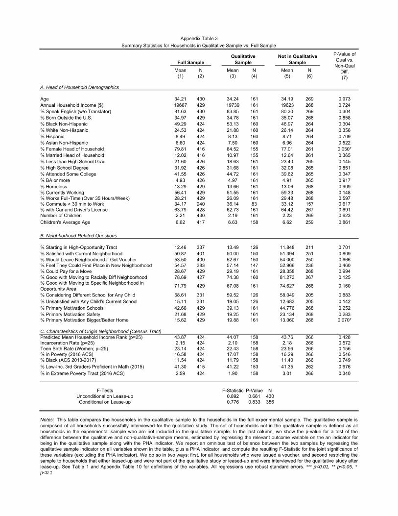
Mean(1)

N(2)

Mean(3)

N(4)

Mean(5)

N(6)

A. Head of Household Demographics

Age 34.21 430 34.24 161 34.19 269 0.973Annual Household Income ($) 19667 429 19739 161 19623 268 0.724% Speak English (w/o Translator) 81.63 430 83.85 161 80.30 269 0.304% Born Outside the U.S. 34.97 429 34.78 161 35.07 268 0.858% Black Non-Hispanic 49.29 424 53.13 160 46.97 264 0.304% White Non-Hispanic 24.53 424 21.88 160 26.14 264 0.356% Hispanic 8.49 424 8.13 160 8.71 264 0.709% Asian Non-Hispanic 6.60 424 7.50 160 6.06 264 0.522% Female Head of Household 79.81 416 84.52 155 77.01 261 0.050*% Married Head of Household 12.02 416 10.97 155 12.64 261 0.365% Less than High School Grad 21.60 426 18.63 161 23.40 265 0.145% High School Degree 31.92 426 31.68 161 32.08 265 0.851% Attended Some College 41.55 426 44.72 161 39.62 265 0.347% BA or more 4.93 426 4.97 161 4.91 265 0.917% Homeless 13.29 429 13.66 161 13.06 268 0.909% Currently Working 56.41 429 51.55 161 59.33 268 0.148% Works Full-Time (Over 35 Hours/Week) 28.21 429 26.09 161 29.48 268 0.597% Commute > 30 min to Work 34.17 240 36.14 83 33.12 157 0.617% with Car and Driver's License 63.79 428 62.73 161 64.42 267 0.691Number of Children 2.21 430 2.19 161 2.23 269 0.623

Children's Average Age 6.62 417 6.63 158 6.62 259 0.861

B. Neighborhood-Related Questions

% Starting in High-Opportunity Tract 12.46 337 13.49 126 11.848 211 0.701% Satisfied with Current Neighborhood 50.87 401 50.00 150 51.394 251 0.809% Would Leave Neighborhood if Got Voucher 53.50 400 52.67 150 54.000 250 0.666% Feel They Could Find Place in New Neighborhood 54.57 383 57.14 147 52.966 236 0.460% Could Pay for a Move 28.67 429 29.19 161 28.358 268 0.994% Good with Moving to Racially Diff Neighborhood 78.69 427 74.38 160 81.273 267 0.125% Good with Moving to Specific Neighborhood in Opportunity Area

71.79 429 67.08 161 74.627 268 0.160

% Considering Different School for Any Child 58.61 331 59.52 126 58.049 205 0.883% Unsatisfied with Any Child's Current School 15.11 331 19.05 126 12.683 205 0.142% Primary Motivation Schools 42.66 429 39.13 161 44.776 268 0.252% Primary Motivation Safety 21.68 429 19.25 161 23.134 268 0.283% Primary Motivation Bigger/Better Home 15.62 429 19.88 161 13.060 268 0.070*

C. Characteristics of Origin Neighborhood (Census Tract) Predicted Mean Household Income Rank (p=25) 43.87 424 44.07 158 43.76 266 0.428Incarceration Rate (p=25) 2.15 424 2.10 158 2.18 266 0.572Teen Birth Rate (Women; p=25) 23.14 424 22.43 158 23.56 266 0.156% in Poverty (2016 ACS) 16.58 424 17.07 158 16.29 266 0.546% Black (ACS 2013-2017) 11.54 424 11.79 158 11.40 266 0.749% Low-Inc. 3rd Graders Proficient in Math (2015) 41.30 415 41.22 153 41.35 262 0.976

% in Extreme Poverty Tract (2016 ACS) 2.59 424 1.90 158 3.01 266 0.340

F-Tests F-Statistic P-Value NUnconditional on Lease-up 0.892 0.661 430Conditional on Lease-up 0.776 0.833 356

Notes: This table compares the households in the qualitative sample to the households in the full experimental sample. The qualitative sample iscomposed of all households successfully interviewed for the qualitative study. The set of households not in the qualitative sample is defined as allhouseholds in the experimental sample who are not included in the qualitative sample. In the last column, we show the p-value for a test of thedifference between the qualitative and non-qualitative-sample means, estimated by regressing the relevant outcome variable on the an indicator forbeing in the qualitative sample along with the PHA indicator. We report an omnibus test of balance between the two samples by regressing thequalitative sample indicator on all variables shown in the table, plus a PHA indicator, and compute the resulting F-Statistic for the joint significance ofthese variables (excluding the PHA indicator). We do so in two ways: first, for all households who were issued a voucher, and second restricting thesample to households that either leased-up and were not part of the qualitative study or leased-up and were interviewed for the qualitative study afterlease-up. See Table 1 and Appendix Table 10 for definitions of the variables. All regressions use robust standard errors. *** p<0.01, ** p<0.05, *p<0.1

Appendix Table 3

Summary Statistics for Households in Qualitative Sample vs. Full Sample

Qualitative Sample

Not in Qualitative SampleFull Sample

P-Value of Qual vs.

Non-Qual Diff.(7)

Mean(1)

N(2)

Mean(3)

N(4)

A. Head of Household Demographics

Age 32.24 42 34.94 119 0.031**Annual Household Income ($) 19047.62 42 19983.19 119 0.782% Speak English (w/o Translator) 83.33 42 84.03 119 0.898% Born Outside the U.S. 33.33 42 35.29 119 0.831% Black Non-Hispanic 57.14 42 51.69 118 0.603% White Non-Hispanic 19.05 42 22.88 118 0.568% Hispanic 9.52 42 7.63 118 0.753% Asian Non-Hispanic 2.38 42 9.32 118 0.069*% Female Head of Household 92.68 41 81.58 114 0.041**% Married Head of Household 9.76 41 11.40 114 0.615% Less than High School Grad 26.19 42 15.97 119 0.243% High School Degree 30.95 42 31.93 119 0.987% Attended Some College 38.10 42 47.06 119 0.303% BA or more 4.76 42 5.04 119 0.953% Homeless 19.05 42 11.76 119 0.332% Currently Working 54.76 42 50.42 119 0.565% Works Full-Time (Over 35 Hours/Week) 28.57 42 25.21 119 0.573% Commute > 30 min to Work 26.09 23 40.00 60 0.328% with Car and Driver's License 52.38 42 66.39 119 0.126Number of Children 2.10 42 2.22 119 0.533Children's Average Age 5.24 42 7.13 116 0.003***

B. Neighborhood-Related Questions

% Starting in High-Opportunity Tract 12.12 33 13.98 93 0.780% Satisfied with Current Neighborhood 46.15 39 51.35 111 0.647% Would Leave Neighborhood if Got Voucher 56.41 39 51.35 111 0.662% Feel They Could Find Place in New Neighborhood 62.50 40 55.14 107 0.458% Could Pay for a Move 33.33 42 27.73 119 0.599% Good with Moving to Racially Diff Neighborhood 83.33 42 71.19 118 0.052*% Good with Moving to Specific Neighborhood in Opportunity Area 66.67 42 67.23 119 0.967% Considering Different School for Any Child 70.00 30 56.25 96 0.169% Unsatisfied with Any Child's Current School 20.00 30 18.75 96 0.888% Primary Motivation Schools 35.71 42 40.34 119 0.603% Primary Motivation Safety 16.67 42 20.17 119 0.541% Primary Motivation Bigger/Better Home 19.05 42 20.17 119 0.897

C. Characteristics of Origin Neighborhood (Census Tract)

Predicted Mean Household Income Rank (p=25) 44.50 41 43.92 117 0.425Incarceration Rate (p=25) 1.92 41 2.16 117 0.320Teen Birth Rate (Women; p=25) 21.34 41 22.81 117 0.337% in Poverty (2016 ACS) 15.75 41 17.53 117 0.302% Black (ACS 2013-2017) 11.37 41 11.94 117 0.722% Low-Inc. 3rd Graders Proficient in Math (2015) 41.99 39 40.96 114 0.624% in Extreme Poverty Tract (2016 ACS) 4.88 41 0.85 117 0.269

F-Tests F-Statistic P-Value NUnconditional on Lease-up 0.854 0.708 161Conditional on Lease-up 0.739 0.850 130

Appendix Table 4

P-Value of T-C

Difference(8)

Summary Statistics for Households in the Qualitative Sample

Control Treatment

Notes: This table replicates the summary statistics in Table 1, but restricts the sample to families who participated in the qualitative survey definedin Appendix Table 3. In addition to the F-Statistic of joint significance using all families who participated in the qualitative study, we show a secondF-Statisctic restricting the sample to households who leased-up and were interviewed after lease-up if they participated in the qualitative study. Allregressions use robust standard errors. See Table 1 for further details. *** p<0.01, ** p<0.05, * p<0.1

(1) Average Upward Mobility (in ranks) in control group destinations

(2) [Translated to 2015 USD] $35,955

(3) Treatment effect (TOT) on Tract-Level Upward Mobility (in ranks)

(4) Estimated causal effect of move from birth [ = 62% of (3)]

(5) Expected Upward Mobility (in ranks) for treated [ = (1) + (4) ]

(6) [Translated to 2015 USD] $38,955

(7) Causal effect of CMTO on yearly income at age 34 (2015 USD) [ = (6) - (2) ]

(8) Avg family income at age 34 (2015 USD, from ACS)

(9) Undiscounted income over the lifecycle from ACS, assuming 1% income growth (2015 USD)

(10) Impact as % of avg family income in ACS [ = (7) / (8) ]

(11) Causal treatment effect on undiscounted lifetime income (USD) [ = (10) * (9) ]

(12) Avg undiscounted income over the lifecycle for low-income children in Seattle area (2015 USD)

(13) Impact as % of avg low-income lifetime earnings in Seattle area [ = (11) / (12) ]

(14) Discounted income over the lifecycle from ACS, 1% income growth (2015 USD)

(15) Causal treatment effect on discounted lifetime income (USD) [ = (10) * (14) ]

$1,825,930

$85,394

Notes: This table outlines the steps we use to translate our estimated treatment effects into lifetime earnings effects for thechildren whose families moved to high-opportunity neighborhoods as a result of CMTO. We estimate the impact on incomes fora child that moved to a high-opportunity neighborhood at birth. Row (1) presents the average level of upward mobility in thedestination tracts to which families in the control group moved using data from the Opportunity Atlas (i.e. the family income rankat age 34 of children in the 1978-83 birth cohorts, based on their childhood neighborhood, for families at the 25th percentile ofthe parental income distribution). Row (2) translates this level into 2015 USD by mapping this percentile to dollars using thenational income distribution for 31-37 year olds in 2014-2015. Row (3) presents the treatment effect of CMTO on upwardmobility for those who moved to an opportunity neighborhood (TOT). Row (4) multiplies this effect by 62%, based on theestimate from Chetty et al. (2018) that children who move at birth to a neighborhood with 1 rank higher upward mobility grow upto have an income rank that is 0.62 units higher. Row (5) presents the sum of this effect and the control group mean. Row (6)translates this into 2015 USD using the same approach as in Row (2). Row (7) computes the difference in expected incomelevels between the treated and untreated groups. Row (8) reports the mean family income (individual income plus spousalincome for married couples, to match our measure of family income in the Opportunity Atlas) from the 2015 ACS at age 34.Row (9) presents the undiscounted sum of mean family income in the 2015 ACS, summing across all ages and assuming 1%wage growth from birth. Row (10) computes the percentage impact on incomes by dividing (7) by (8). Row (11) computes theimpact on lifetime undiscounted income assuming the percentage impact on income over the life cycle is constant. Row (12)reports an estimate of the undiscounted mean family income over the lifecycle for children born to parents in the 25th percentileof the national income distribution who grew up in a low-opportunity area in Seattle and King County. We estimate this value bymutiplying the mean income for children growing up in low-income (25th percentile) families in low-opportunity areas in Seattleand King County by row (9) divided by row (8). Row (13) reports the earnings gain from moving to a high-opportunity area as apercentage of mean income for children growing up in low-income families in low-opportunity areas in Seattle and King Countyby dividing (11) by (12). Rows (14) and (15) compute the impact on discounted lifetime income. Row (14) reports mean lifetimeincome in the ACS discounted over the life cycle at 2%, assuming 1% income growth from birth. Row (15) reports the impact ondiscounted lifetime income, again assuming the percentage impact over the life cycle is constant.

47.17

$3,001

$64,160

4.68%

$4,585,149

$214,436

$2,539,340

8.44%

2.64

4.25

Appendix Table 5Calculation of Lifetime Earnings Impact of CMTO

44.53

Control Mean

Treatment Mean

Treatment Effect

SE N P-Value

(1) (2) (3) (4) (5) (6)

A. Pooled and by Housing Authority

All Families 85.9 87.3 1.5 3.3 427 0.662All Families (Controls) 85.9 87.0 1.1 3.4 427 0.739Seattle Housing Authority 85.1 86.0 0.9 5.0 201 0.864King County Housing Authority 86.5 88.5 2.0 4.4 226 0.655

B. By Head of Household Demographic Characteristics

Black Non-Hispanic 87.1 90.3 3.2 4.5 208 0.479White Non-Hispanic 84.8 85.4 0.6 7.0 103 0.927Other Race/Ethnicity 85.7 84.2 -1.6 6.9 111 0.823Born Outside the U.S. 85.9 89.2 3.3 5.4 150 0.538Born in the U.S. 85.7 87.0 1.3 4.2 276 0.758English Isn't Primary Language 87.2 92.9 5.8 6.9 80 0.403English Is Primary Language 85.5 86.0 0.6 3.8 346 0.87620 years or more in Seattle/King County 88.4 86.3 -2.0 4.9 183 0.678Less than 20 years in Seattle/King County 83.9 88.0 4.1 4.5 243 0.363Started in High Opportunity Tract 95.0 95.5 0.5 6.8 42 0.946Didn't Start in High Opportunity Tract 85.9 86.1 0.2 4.1 293 0.969Income ≤ $19,000 (sample median) 85.1 86.0 0.8 4.8 219 0.865Income > $19,000 (sample median) 87.4 89.3 1.9 4.5 207 0.664No College 85.4 87.5 2.1 4.6 226 0.651Some College or More 86.1 86.9 0.8 4.9 197 0.874Currently Working 87.9 87.2 -0.7 4.3 242 0.864Currently Not Working 82.5 87.5 5.0 5.4 184 0.354Uses Child Care 86.1 85.2 -0.9 4.9 211 0.853Doesn't Use Childcare 85.4 88.2 2.8 4.7 215 0.555

C. By Perceptions About Moving at Baseline

Feels Good About Moving to an Opportunity Area 86.5 91.1 4.6 3.6 306 0.197Doesn't Feel Good About Moving to an Opportunity Area 83.9 78.2 -5.7 7.2 120 0.426Satisfied With Current Neighborhood 85.9 87.5 1.6 4.8 203 0.739Unsatisfied/Indifferent With Current Neighborhood 87.9 86.7 -1.2 4.9 195 0.807Sure Wants to Leave Current Neighborhood 88.0 87.5 -0.4 4.6 211 0.927Sure Wants to Stay in Current Neighborhood or Indifferent 86.6 86.2 -0.3 5.0 186 0.944Feels Good About Moving to Racially Different Neighborhood 87.6 87.1 -0.4 3.7 333 0.907Feels Bad/Indifferent About Moving to Racially Different Neighborhood 76.5 87.5 11.0 8.7 91 0.205Sure Could Pay for Moving Expenses 82.1 85.8 3.8 6.7 123 0.577Not Sure Could Pay for a Moving Expenses 87.6 87.9 0.3 3.8 303 0.935Sure Could Find a New Place 85.6 89.2 3.7 4.6 207 0.425Not Sure Could Find a New Place 87.2 86.3 -0.9 5.2 173 0.866

D. By Children's Characteristics

Mean Children Age at or Above Median (6.3 years) 81.8 86.0 4.2 5.1 207 0.410Mean Children Age Below Median (6.3 years) 89.8 88.0 -1.7 4.5 207 0.697More than 2 Children 88.1 84.8 -3.3 6.0 137 0.5872 Children or Less 84.8 88.9 4.1 4.1 290 0.311Considering Different Schools 83.2 84.6 1.4 5.4 192 0.792Not Considering Different Schools 86.9 84.9 -2.0 5.9 137 0.741

Lease-up Rates (%)

Appendix Table 6Heterogeneity of Treatment Effects on Lease-up Rates

Notes: This table replicates Table 2 using an indicator for leasing up anywhere using one's voucher as the outcome instead of leasingup in a high-opportunity area. See Table 2 for details. *** p<0.01, ** p<0.05, * p<0.1

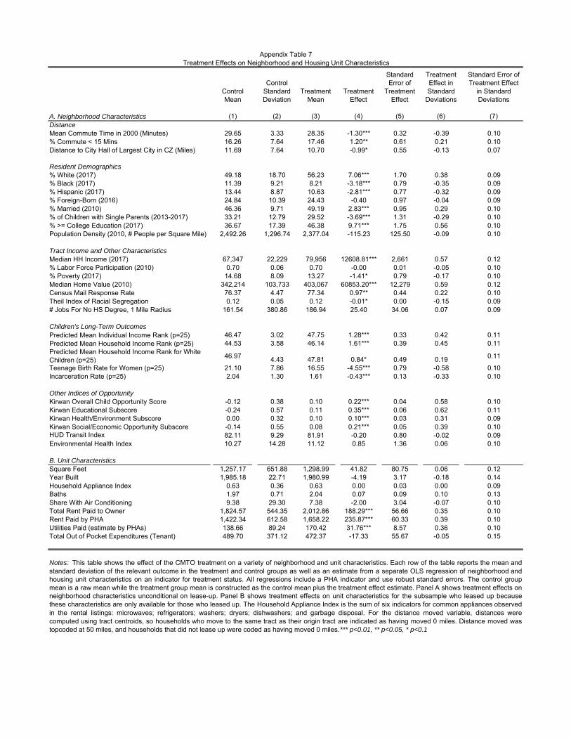
A. Neighborhood Characteristics

Control Mean

(1)

Control Standard Deviation

(2)

Treatment Mean

(3)

Treatment Effect

(4)

Standard Error of

Treatment Effect

(5)

Treatment Effect in Standard

Deviations

(6)

Standard Error of Treatment Effect

in Standard Deviations

(7)DistanceMean Commute Time in 2000 (Minutes) 29.65 3.33 28.35 -1.30*** 0.32 -0.39 0.10% Commute < 15 Mins 16.26 7.64 17.46 1.20** 0.61 0.21 0.10Distance to City Hall of Largest City in CZ (Miles) 11.69 7.64 10.70 -0.99* 0.55 -0.13 0.07

Resident Demographics% White (2017) 49.18 18.70 56.23 7.06*** 1.70 0.38 0.09% Black (2017) 11.39 9.21 8.21 -3.18*** 0.79 -0.35 0.09% Hispanic (2017) 13.44 8.87 10.63 -2.81*** 0.77 -0.32 0.09% Foreign-Born (2016) 24.84 10.39 24.43 -0.40 0.97 -0.04 0.09% Married (2010) 46.36 9.71 49.19 2.83*** 0.95 0.29 0.10% of Children with Single Parents (2013-2017) 33.21 12.79 29.52 -3.69*** 1.31 -0.29 0.10% >= College Education (2017) 36.67 17.39 46.38 9.71*** 1.75 0.56 0.10Population Density (2010, # People per Square Mile) 2,492.26 1,296.74 2,377.04 -115.23 125.50 -0.09 0.10

Tract Income and Other CharacteristicsMedian HH Income (2017) 67,347 22,229 79,956 12608.81*** 2,661 0.57 0.12% Labor Force Participation (2010) 0.70 0.06 0.70 -0.00 0.01 -0.05 0.10% Poverty (2017) 14.68 8.09 13.27 -1.41* 0.79 -0.17 0.10Median Home Value (2010) 342,214 103,733 403,067 60853.20*** 12,279 0.59 0.12Census Mail Response Rate 76.37 4.47 77.34 0.97** 0.44 0.22 0.10Theil Index of Racial Segregation 0.12 0.05 0.12 -0.01* 0.00 -0.15 0.09# Jobs For No HS Degree, 1 Mile Radius 161.54 380.86 186.94 25.40 34.06 0.07 0.09

Children's Long-Term OutcomesPredicted Mean Individual Income Rank (p=25) 46.47 3.02 47.75 1.28*** 0.33 0.42 0.11Predicted Mean Household Income Rank (p=25) 44.53 3.58 46.14 1.61*** 0.39 0.45 0.11Predicted Mean Household Income Rank for White Children (p=25)

46.97 4.43 47.81 0.84* 0.49 0.19 0.11

Teenage Birth Rate for Women (p=25) 21.10 7.86 16.55 -4.55*** 0.79 -0.58 0.10Incarceration Rate (p=25) 2.04 1.30 1.61 -0.43*** 0.13 -0.33 0.10

Other Indices of OpportunityKirwan Overall Child Opportunity Score -0.12 0.38 0.10 0.22*** 0.04 0.58 0.10Kirwan Educational Subscore -0.24 0.57 0.11 0.35*** 0.06 0.62 0.11Kirwan Health/Environment Subscore 0.00 0.32 0.10 0.10*** 0.03 0.31 0.09Kirwan Social/Economic Opportunity Subscore -0.14 0.55 0.08 0.21*** 0.05 0.39 0.10HUD Transit Index 82.11 9.29 81.91 -0.20 0.80 -0.02 0.09Environmental Health Index 10.27 14.28 11.12 0.85 1.36 0.06 0.10

B. Unit CharacteristicsSquare Feet 1,257.17 651.88 1,298.99 41.82 80.75 0.06 0.12Year Built 1,985.18 22.71 1,980.99 -4.19 3.17 -0.18 0.14Household Appliance Index 0.63 0.36 0.63 0.00 0.03 0.00 0.09Baths 1.97 0.71 2.04 0.07 0.09 0.10 0.13Share With Air Conditioning 9.38 29.30 7.38 -2.00 3.04 -0.07 0.10Total Rent Paid to Owner 1,824.57 544.35 2,012.86 188.29*** 56.66 0.35 0.10Rent Paid by PHA 1,422.34 612.58 1,658.22 235.87*** 60.33 0.39 0.10Utilities Paid (estimate by PHAs) 138.66 89.24 170.42 31.76*** 8.57 0.36 0.10Total Out of Pocket Expenditures (Tenant) 489.70 371.12 472.37 -17.33 55.67 -0.05 0.15

Notes: This table shows the effect of the CMTO treatment on a variety of neighborhood and unit characteristics. Each row of the table reports the mean andstandard deviation of the relevant outcome in the treatment and control groups as well as an estimate from a separate OLS regression of neighborhood andhousing unit characteristics on an indicator for treatment status. All regressions include a PHA indicator and use robust standard errors. The control groupmean is a raw mean while the treatment group mean is constructed as the control mean plus the treatment effect estimate. Panel A shows treatment effects onneighborhood characteristics unconditional on lease-up. Panel B shows treatment effects on unit characteristics for the subsample who leased up becausethese characteristics are only available for those who leased up. The Household Appliance Index is the sum of six indicators for common appliances observedin the rental listings: microwaves; refrigerators; washers; dryers; dishwashers; and garbage disposal. For the distance moved variable, distances werecomputed using tract centroids, so households who move to the same tract as their origin tract are indicated as having moved 0 miles. Distance moved wastopcoded at 50 miles, and households that did not lease up were coded as having moved 0 miles. *** p<0.01, ** p<0.05, * p<0.1

Appendix Table 7Treatment Effects on Neighborhood and Housing Unit Characteristics

All Tracts(1)

Non-High-Opportunity

Tracts(2)

High-Opportunity

Tracts (3)

Z-Score for(4)-(3)

(5)DistanceMean Commute Time in 2000 (Minutes) 29.01 29.62 26.86 27.08 0.05% Commute < 15 Mins 17.47 17.14 18.65 18.12 -0.08Distance to City Hall of Largest City in CZ (Miles) 11.84 12.21 10.51 9.53 -0.14

Resident Demographics% White (2017) 53.81 51.16 63.17 63.01 -0.01% Black (2017) 9.11 10.74 3.35 4.48 0.13% Hispanic (2017) 12.78 14.36 7.20 7.28 0.01% Foreign-Born (2016) 24.19 23.99 24.90 23.82 -0.09% Married (2010) 50.24 48.29 57.14 53.48 -0.34% of Children with Single Parents (2013-2017) 29.61 32.60 19.05 22.57 0.25% >= College Education (2017) 39.33 34.21 57.46 58.80 0.07Population Density (2010, # People per Square Mile) 2174.42 2255.41 1887.98 2081.69 0.12

Tract Income and Other CharacteristicsMedian HH Income (2017) 75,986.53 68,269.98 103,276.59 98,259.67 -0.17% Labor Force Participation (2010) 69.80 69.82 69.76 70.35 0.10% Poverty (2017) 13.00 14.32 8.35 9.97 0.19Median Home Value (2010) 366,668.91 334,382.78 481,908.56 479,475.22 -0.02Census Mail Response Rate 77.29 76.57 79.84 78.47 -0.25Theil Index of Racial Segregation 0.13 0.14 0.12 0.11 -0.20# Jobs For No HS Degree, 1 Mile Radius 189.62 199.07 156.21 170.26 0.04

Children's Long-Term OutcomesPredicted Mean Individual Income Rank (p=25) 46.73 45.70 50.37 49.74 -0.16Predicted Mean Household Income Rank (p=25) 45.50 44.16 50.27 48.54 -0.37

Teenage Birth Rate for Women (p=25) 19.67 22.06 11.25 10.79 -0.06

Incarceration Rate (p=25) 1.92 2.11 1.28 1.20 -0.05

Other Indices of OpportunityKirwan Child Opportunity Index - Overall Score -0.04 -0.15 0.34 0.37 0.06Kirwan Child Opportunity Index - Educational Subscore -0.13 -0.31 0.51 0.54 0.04Kirwan Child Opportunity Index - Health/Environment Subscore 0.05 0.02 0.16 0.20 0.16Kirwan Child Opportunity Index - Social/Economic Subscore -0.05 -0.17 0.35 0.36 0.02HUD Transit Index 79.56 79.72 78.99 81.00 0.18Environmental Health Index 13.22 12.50 15.53 14.21 -0.07

Notes: This table shows neighborhood characteristics for different groups of Census tracts. The first three columns show means (weighted by the numberof people in the 2000 Decennial Census with below median income) for all tracts, low-opportunity tracts, and high-opportunity tracts, respectively. Thefourth column shows means for high-opportunity tracts to which CMTO participants moved, weighted by the number of CMTO participants who moved toeach tract. The final column shows the Z-score of the difference between the weighted average for all high opportunity tracts and the weighted average ofhigh opportunity tracts to which CMTO families moved. Data on commute times come from the 2000 Decennial Census (mean commute time) and fromthe 2012-2016 ACS (% commute time < 15 min), resident demographics and tract income from the ACS; children's long-term outcomes from theOpportunity Atlas; and other indices of opportunity from The Kirwan Child Opportunity Index constructed by The Kirwan Institute for the Study of Race andEthnicity and from HUD's Affirmatively Furthering Fair Housing Data and Mapping Tool (AFFH-T).

Appendix Table 8

Neighborhood Characteristics of High vs. Low Opportunity Areas

Tract Means, Weighted by Num. of. Children in Below Median Income Families

High-Opportunity Tracts Moved Into

By CMTO Participants

(4)

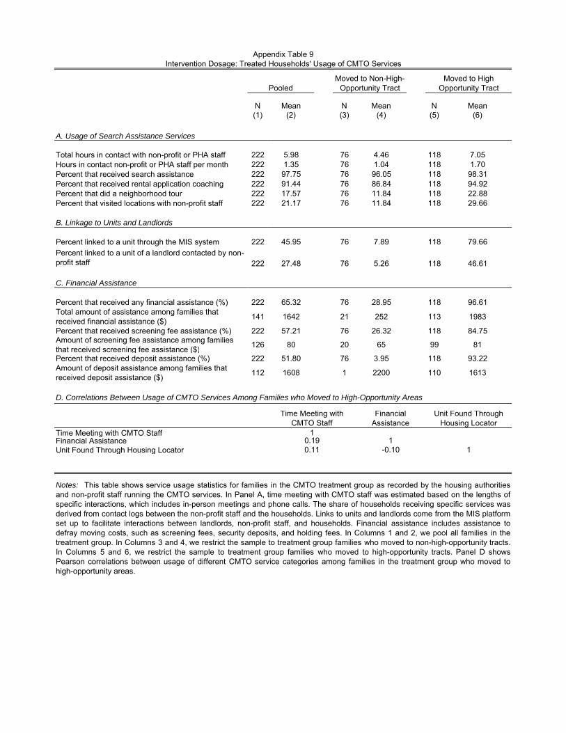
N Mean N Mean N Mean(1) (2) (3) (4) (5) (6)

A. Usage of Search Assistance Services

Total hours in contact with non-profit or PHA staff 222 5.98 76 4.46 118 7.05Hours in contact non-profit or PHA staff per month 222 1.35 76 1.04 118 1.70Percent that received search assistance 222 97.75 76 96.05 118 98.31Percent that received rental application coaching 222 91.44 76 86.84 118 94.92Percent that did a neighborhood tour 222 17.57 76 11.84 118 22.88Percent that visited locations with non-profit staff 222 21.17 76 11.84 118 29.66

B. Linkage to Units and Landlords

Percent linked to a unit through the MIS system 222 45.95 76 7.89 118 79.66

Percent linked to a unit of a landlord contacted by non-profit staff 222 27.48 76 5.26 118 46.61

C. Financial Assistance

Percent that received any financial assistance (%) 222 65.32 76 28.95 118 96.61Total amount of assistance among families that received financial assistance ($)

141 1642 21 252 113 1983

Percent that received screening fee assistance (%) 222 57.21 76 26.32 118 84.75Amount of screening fee assistance among families that received screening fee assistance ($)

126 80 20 65 99 81

Percent that received deposit assistance (%) 222 51.80 76 3.95 118 93.22Amount of deposit assistance among families that received deposit assistance ($)

112 1608 1 2200 110 1613

D. Correlations Between Usage of CMTO Services Among Families who Moved to High-Opportunity Areas

Time Meeting with CMTO StaffFinancial AssistanceUnit Found Through Housing Locator

Notes: This table shows service usage statistics for families in the CMTO treatment group as recorded by the housing authoritiesand non-profit staff running the CMTO services. In Panel A, time meeting with CMTO staff was estimated based on the lengths ofspecific interactions, which includes in-person meetings and phone calls. The share of households receiving specific services wasderived from contact logs between the non-profit staff and the households. Links to units and landlords come from the MIS platformset up to facilitate interactions between landlords, non-profit staff, and households. Financial assistance includes assistance todefray moving costs, such as screening fees, security deposits, and holding fees. In Columns 1 and 2, we pool all families in thetreatment group. In Columns 3 and 4, we restrict the sample to treatment group families who moved to non-high-opportunity tracts.In Columns 5 and 6, we restrict the sample to treatment group families who moved to high-opportunity tracts. Panel D showsPearson correlations between usage of different CMTO service categories among families in the treatment group who moved tohigh-opportunity areas.

Financial Assistance

1-0.10

Time Meeting with CMTO Staff

10.190.11

Unit Found Through Housing Locator

1

PooledMoved to Non-High-

Opportunity TractMoved to High

Opportunity Tract

Appendix Table 9Intervention Dosage: Treated Households' Usage of CMTO Services

Survey Instrument Reference Variable Coding Details

% Speak EnglishQ7. Is an interpreter or translation service being used for survey administration?

% Born Outside the U.S. Q10. In what country were you born?

% Less than High School GradQ22. What is the highest level of education that you have completed?

= Grade 9 or less OR Grade 10 or grade 11 OR Attended grade 12 but did not receive high school diploma or GED certificate

% High School DegreeQ22. What is the highest level of education that you have completed?

= GED certificate OR High school diploma

% Attended Some CollegeQ22. What is the highest level of education that you have completed?

= Some college or Associate’s or two-year degree

% BA or moreQ22. What is the highest level of education that you have completed?

= Four-year college degree or higher

% Homeless Q14. Where do you currently live? = Homeless or in a group shelter

% Currently Working Q15. Are you currently working for pay?

% Commute > 30 min to Work Q17. How long does it take you to get to your job?= 31 to 45 minutes OR 46 minutes to one hour OR More than one hour

% with Car and Driver's LicenseQ19. Do you have a valid driver’s license? AND Q20. Do you have access to a car that runs?

% Satisfied with Current NeighborhoodQ32. Which of the following statements best describes how satisfied you are with your current neighborhood?

= Very satisfied OR Somewhat satisfied

% Would Leave Neighborhood if Got Voucher

Q33. Which of the following statements best describes how you feel about staying in your current neighborhood if you receive a voucher?

= Somewhat sure I want to move to a different neighborhood OR Very sure I want to move to a different neighborhood

% Feel They Could Find Place in New Neighborhood

Q47: How sure are you that you could find a home in a new neighborhood in [Seattle/King County]?

= Very sure OR Fairly sure

% Could Pay for a MoveQ50. How sure are you that you will be able to pay for any moving expenses?

= Very sure OR Fairly sure

% Good with moving to Racially Diff Neighborhood

Q43. How would you feel about moving to a neighborhood where almost all of the other residents are of a different race or ethnicity than your own?

= Very good OR Good

% Good with Moving to Specific Neighborhood in Opportunity Area

Q36. If a home or apartment were to be available, how would you feel about moving to ___? Would you feel… AND Q39. How would you feel about moving to ___? AND Q42. How would you feel about moving to neighborhoods ___?

= Very good OR Good [in at least one of the questions]

Number of Children Remind me how many children do you have?Children's Average Age Q53. What is the child’s age?

% Considering Different School for Any Child

Q58. Are you currently considering transferring him/her to a different school (or Pre-K/Pre-school program)?

= Yes [for at least one child]

% Unsatisfied with Any Child's Current School

Q57. How satisfied are you with his/her current school (or Pre-K/Pre-school program)?

= Somewhat unsatisfied OR Very unsatisfied [for at least one child]

20 years or more in Seattle/King CountyQ13. How long have you lived in the Seattle or King County area in your lifetime?

Uses Child CareQ27. What types of child care do you use for your child or children? (Check all that apply)

Feels Good About Moving to an Opportunity Area

see % Good with Moving to Specific Neighborhood in Opportunity Area

Sure Wants to Leave Current Neighborhood

see % Would Leave Neighborhood if Got Voucher

Sure Could Find a New Place see % Feel They Could Find Place in New Neighborhood

% Black / Hispanic / Latino / White3k. Use code or codes at bottom of page that the family says best indicates each household member’s race. Select as many codes as appropriate

Income < $19,000 19h:The total dollar amounts listed in column 19f. Note: 19f is income minus exclusions

Notes: This table presents definitions of the variables, which come from the baseline survey and from PHA administrative data (HUD form 50058).The baseline questionnaire can be found here.

A. Baseline Variables

B. Public Housing Authority Data

Appendix Table 10Baseline Survey Questions and Coding of Variables

FIGURE 1: The Geography and Price of Opportunity in Seattle

A. Upward Mobility by Census Tract in Seattle and King County

25 most common tracts where voucher holders leased units before the CMTO experiment

> 57 ($51k)

48 ($40k)

< 36 ($27k)

Mean Household Income Rank in Adulthood

This map must be printed in color to be interpretable

B. Upward Mobility vs. Median Rent, by Tract

West KentFederal Way

Newport

Woodinville

$21K 30

$31K 40

$42K 50

$56K 60

Mea

n H

ouse

hold

Inco

me

Ran

ks o

f Chi

ldre

nw

ith L

ow-In

com

e (2

5th

Perc

enct

ile) P

aren

ts

$500 $1,000 $1,500 $2,000 $2,500 Median 2-Bedroom Rent in 2015

Notes: The map in Panel A shows the Opportunity Atlas estimates of upward mobility, defined as the mean predictedhousehold income rank in 2014-15 for children whose parents were at the 25th percentile of the national household incomedistribution (an income of $27,000) for children in the 1978-1983 birth cohorts. This measure is estimated separately in eachtract as described in Chetty, Friedman, Hendren, Jones, and Porter (2018). To facilitate interpretation of the percentile ranks,we also show the dollar value corresponding to each percentile shown in the legend based on the income distribution of childrenin the 1978-83 birth cohorts. Green dots show the 25 most common tracts where families with children leased units usinga Housing Choice Voucher administered by the King County or Seattle housing authorities in 2015-2017, before the CMTOexperiment (based on voucher household shares of the total tract population in 2010). Panel B presents a scatter plot ofupward mobility in each tract vs. median rent for two-bedroom, renter-occupied units surveyed in the 2011-2015 AmericanCommunity Survey. The inner numbers on the vertical axis show the Opportunity Atlas estimates of mean household incomeranks depicted in Panel A, while the outer numbers on the vertical axis convert those ranks to 2015 dollars based on theincome distribution for children in the 1978-83 birth cohorts. The darker points show 18 of the 25 tracts highlighted in PanelA, which include Federal Way and West Kent (seven of the 25 most common tracts are not shown due to missing rental data).The black best-fit line is estimated using a regression of upward mobility on median rent for two-bedroom homes, weighted bythe number of children growing up in households below the 50th percentile of the national income distribution in each tract.Woodinville and Newport, denoted by hollow points, are examples of tracts with rents comparable to Federal Way and WestKent but offer much better prospects for upward mobility for children.

FIGURE 2: Definition of High-Opportunity NeighborhoodsA. CMTO High-Opportunity Neighborhoods

High-Opportunity Area

Seattle City Boundary

Capitol Hill

West Seattle

RainierValley

Des Moines

Magnolia

Northeast Seattle

NewportCougar

Mountain

Lea Hill, Auburn

East Hill

Inglewood

Bellevue

Issaquah

Lake City

Kent

TukwilaBurien

Redmond

Cottage Lake

Shoreline

Federal Way

Ballard

B. Comparing Alternative Measures of Opportunity

Kirwan Child Opportunity IndexOpportunity Atlas Upward Mobility

Population-Weighted Correlation Across Tracts: 0.30

> 57 ($51k)

48($40k)

< 36 ($27k)

> 0.80 SD 0.35 SD< 0.53 SD

These maps must be printed in color to be interpretable

Notes: Panel A shows the tracts designated as high-opportunity areas in the CMTO experiment, which are shown in bluecross-hatch. Panel B compares upward mobility as defined in the Opportunity Atlas (replicating Panel A of Figure 1) tothe Kirwan Child Opportunity Index. The Kirwan Child Opportunity Index is constructed by The Kirwan Institute for theStudy of Race and Ethnicity and combines 19 components measured between 2007 and 2013 from three subject domains(Educational Opportunity, Health and Environmental Opportunity, and Social and Economic Opportunity), into a singleindex. The population-weighted correlation between the two measures across tracts in King County is 0.30.

FIGURE 3: CMTO Program Structure

A. Key Elements of the Intervention

I N C R E A S E D L A N D L O R D

E N G A G E M E N T

S H O R T - T E R M F I N A N C I A L

A S S I S TA N C E

C U S T O M I Z E DS E A R C H

A S S I S TA N C E

• High-opportunity area education to increase families’ knowledge about high-opportunity areas.

• Rental application coaching to increase families’ competitiveness for rental units by addressing credit history and preparing a narrative.

• Housing locator services to help families identify suitable units in high-opportunity areas.

• Cultivate relationships with landlords in designated high-opportunity areas to create housing opportunities for CMTO families.

• Expedite lease-up processes by completing PHA required documents and conducting housing inspections more quickly.

• Insurance fund to mitigate risks of property damage.

• Grants to defray move-in expenses, such as application fees and security deposits (on average $1,000).

B. Intervention Process Timeline

Family ContactedNotified of selection

from waitlist

Intake Appointment

ConsentRandomizationBaseline survey

Nonprofit Staff Meet with Families and Landlords

Unit SelectedFamily approved by

landlord for unit

Lease UpReceive paperwork and

financial assistance (e.g. assistance for deposit)

Lease Signed

Voucher Issued

Rental application coachingOpportunity area education

Visiting locations

Search assistanceLandlord recruitment

Linking families to units

PHA Nonprofit Family Milestone

Notes: Panel A of this figure describes the key components of the CMTO intervention. Panel B presents a stylized timelineof the treatment intervention from the perspective of a family in the treatment group.

FIGURE 4: CMTO Treatment Effects on Neighborhood Choice

A. Fraction Who Lease Units in High-Opportunity Areas

15.1%

53.0%

Historical meanrate: 11.6%

010

2030

4050

60

Shar

e of

Hou

seho

lds

Who

Hav

e M

oved

to H

igh

Opp

ortu

nity

Are

as

Control TreatmentDifference: 37.9 pp SE: (4.2)

B. Fraction who Leased Up Before Voucher Expiration

85.9% 87.4%

020

4060

8010

0

Shar

e of

Hou

seho

lds

Who

Hav

e M

oved

Control TreatmentDifference: 1.5 pp SE: (3.3)

C. Fraction Who Lease Units in High-Opportunity Areas, Conditionalon Leasing Up Somewhere

17.6%

60.7%

020

4060

Shar

e of

Hou

seho

lds

Who

Hav

e M

oved

to H

igh

Opp

ortu

nity

Are

as, G

iven

The

y M

oved

Control TreatmentDifference: 43.1 pp SE: (4.6)

D. Upward Mobility in Destination Tract

44.5

46.140

4244

4648

50

Mea

n H

ouse

hold

Inco

me

Ran

k (p

=25)

in N

eigh

borh

ood

Control TreatmentDifference: 1.6 ranks SE: (0.4)

Notes: This figure shows the treatment effects of the CMTO program on families’ neighborhood choices. Panel A presents thetreatment effect on the fraction who lease up a unit in a high-opportunity tract, as defined in Figure 2. The dashed line inPanel A shows the fraction of voucher recipients who leased units in high-opportunity areas between 2015 and 2017. Panel Bpresents the treatment effect on leasing up in any area prior to voucher expiration. Panel C presents the treatment effect onleasing up in a high-opportunity area conditional on leasing up somewhere. Panel D presents the treatment effect on upwardmobility in the destination, as measured in the Opportunity Atlas, unconditional on lease-up (assigning upward mobility in theorigin tract to households who did not lease up). In all panels, the control mean is calculated as the mean within householdsin the control group. Treatment effects, reported below each panel, are estimated using an OLS regression of the outcome on atreatment indicator and an indicator for being in KCHA/SHA (since randomization occurred within each housing authority).The treatment mean plotted is calculated as the control mean plus the estimated treatment effect. Standard errors reportedare robust standard errors. Panels A, B, and D use the full sample, excluding three households whose voucher was transferredto a different public housing authority (other than KCHA/SHA). Panel C further restricts the sample to the 370 householdswho leased up somewhere using their voucher before it expired. All panels focus on the outcome of the first lease-up aftervoucher issuance.

FIGURE 5: Map of Destination Tracts for Voucher Recipients

High-Opportunity Area

West Seattle

RainierValley

Des Moines

MagnoliaNortheast Seattle

NewportCougar

Mountain

Lea Hill, Auburn

East Hill

Inglewood

Bellevue

Issaquah

Lake City

Kent

TukwilaBurien

Control

CMTOTreatment

Federal Way

Capitol Hill

Ballard

Notes: This figure presents a map of the destination tracts for families in the CMTO treatment and the control groups whomoved using their vouchers. High-opportunity areas are highlighted in blue cross-hatch. We focus on the destination tract ofthe first lease-up after voucher issuance. We exclude 5 households whose vouchers were transferred to different public housingauthorities (3 households) or who used their vouchers to lease up units outside of King County (2 households). To protectconfidentiality, we add a small amount of random noise to the destination tract centroids shown in the maps.

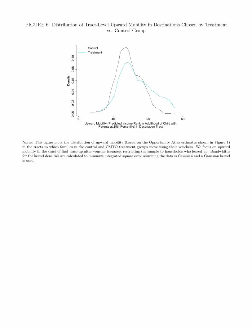
FIGURE 6: Distribution of Tract-Level Upward Mobility in Destinations Chosen by Treatmentvs. Control Group

0.00

0.02

0.04

0.06

0.08

0.10

Den

sity

30 40 50 60Upward Mobility (Predicted Income Rank in Adulthood of Child with

Parents at 25th Percentile) in Destination Tract

ControlTreatment

Notes: This figure plots the distribution of upward mobility (based on the Opportunity Atlas estimates shown in Figure 1)in the tracts to which families in the control and CMTO treatment groups move using their vouchers. We focus on upwardmobility in the tract of first lease-up after voucher issuance, restricting the sample to households who leased up. Bandwidthsfor the kernel densities are calculated to minimize integrated square error assuming the data is Gaussian and a Gaussian kernelis used.

FIGURE 7: Heterogeneity in Treatment Effects

A. Treatment Effects by Race and Ethnicity

Diff. = 36.7 Diff. = 42.7 Diff. = 36.4(5.8) (9.0) (8.6)

10.9%

47.6%

19.6%

62.3%

19.6%

56.0%0

2040

6080

Perc

ent o

f Hou

seho

lds

Who

Mov

edto

Hig

h O

ppor

tuni

ty A

reas

ControlBlack Non-Hispanic

Treatment ControlWhite Non-Hispanic

Treatment ControlOther Race/Ethnicity

Treatment

B. Treatment Effects by Income

Diff. = 36.6 Diff. = 39.2(6.0) (6.0)

16.8%

53.4%

13.6%

52.8%

010

2030

4050

6070

Perc

ent o

f Hou

seho

lds

Who

Mov

edto

Hig

h O

ppor

tuni

ty A

reas

ControlIncome < $19,000

Treatment ControlIncome > $19,000

Treatment

Notes: This figure presents estimates of treatment effects on the share of households moving to high-opportunity areas byrace/ethnicity (Panel A) and baseline income level (Panel B) of the voucher recipient. Treatment and control means areestimated separately within each subgroup following exactly the same method used to construct the pooled estimates reportedin Panel A of Figure 4; see notes to that figure for further details. Panel A uses the 98% of participants who report their raceand Panel B uses the 99% who report their income. The cutoff used in Panel B ($19,000) to divide the two groups correspondsto the median income of the participants in the experiment.

FIGURE 8: Treatment Effects on Neighborhood and Unit Quality

A. Distance Moved

10.511.4

05

1015

Mea

n D

ista

nce

in M

iles

Betw

een

Orig

in a

nd D

estin

atio

n Tr

act C

ente

rs

Control TreatmentDifference: 0.9 miles SE: (1.2)

B. Unit Size

1257.2 1299.0

050

010

0015

00

Squa

re F

eet o

f Hom

e

Control TreatmentDifference: 41.8 sq. feet SE: (80.8)

C. Total Rent Paid to Owner

$1,824.57

$2,012.86

1000

1400

1800

2200

Mon

thly

Ren

t ($)

Control TreatmentDifference: $188.29 SE: (56.7)

Notes: This figure shows treatment effects on the distance moved, square footage of the unit families lease, and the total rentpaid to the property owner for the unit. Distance is calculated as the distance between the centroid of the tract in which thevoucher recipient lived at baseline and the centroid of the tract to which they moved. We topcode distance at 50 miles toreduce the influence of outliers. Treatment and control means are estimated among the subsample of households who leasedup following exactly the same method used to construct the pooled estimates reported in Panel C of Figure 4; see notes tothat figure for further details.

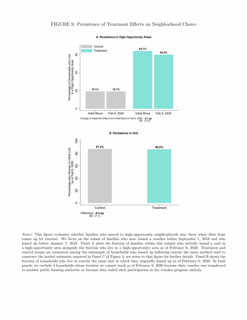
FIGURE 9: Persistence of Treatment Effects on Neighborhood Choice

A. Persistence in High-Opportunity Areas

19.1%

64.1%

19.1%

60.0%

020

4060

Perc

enta

ge o

f Hou

seho

lds

who

Liv

ein

a H

igh

Opp

ortu

nity

Are

a

Initial Move Feb 6, 2020 Initial Move Feb 6, 2020

ControlTreatment

Change in Treatment Effect from Initial Move to Feb 6, 2020: -4.1 pp SE: (13.3)

B. Persistence in Unit

87.2% 86.8%

020

4060

8010

0

Perc

enta

ge w

ho R

emai

n in

Initi

al U

nit

as o

f Feb

6, 2

020

Control TreatmentDifference: -0.4 pp SE: (7.1)

Notes: This figure evaluates whether families who moved to high-opportunity neighborhoods stay there when their leasecomes up for renewal. We focus on the subset of families who were issued a voucher before September 1, 2018 and wholeased up before January 7, 2019. Panel A plots the fraction of families within this sample who initially leased a unit ina high-opportunity area alongside the fraction who live in a high-opportunity area as of February 6, 2020. Treatment andcontrol means are estimated among the subsample of households who leased up following exactly the same method used toconstruct the pooled estimates reported in Panel C of Figure 4; see notes to that figure for further details. Panel B shows thefraction of households who live in exactly the same unit in which they originally leased up as of February 6, 2020. In bothpanels, we exclude 4 households whose location we cannot track as of February 6, 2020 because their voucher was transferredto another public housing authority or because they ended their participation in the voucher program entirely.

FIGURE 10: Treatment Effects on Post-Move Neighborhood Satisfaction

A. Satisfaction with New Neighborhood

45.5%

64.2%

020

4060

80

Shar

e Ve

ry S

atis

fied

with

New

Nei

ghbo

rhoo

d

Control TreatmentDifference: 18.7 pp SE: (10.1)

B. Certainty About Wanting to Stay in New Neighborhood

30.3%

47.7%

020

4060

Shar

e Ve

ry S

ure

They

Will

Stay

in N

ew N

eigh

borh

ood

Control TreatmentDifference: 17.4 pp SE: (9.8)

Notes: This figure shows treatment effects using data from a follow-up qualitative survey administered to a random sampleof CMTO participants. Panel A shows treatment effects on measures of neighborhood satisfaction. Participants were asked,“Which of the following statements best describes how satisfied you are with your current neighborhood? 1. Very Satisfied -2. Somewhat satisfied - 3. In the middle - 4. Somewhat dissatisfied - 5. Very dissatisfied - 6. (No Answer).” Panel B presentsmeasures of the certainty with which participants want to stay in their new neighborhood. Participants were asked, “Whichof the following statements best describes how you feel about staying in your current neighborhood? - 1. Very sure I want tostay - 2. Somewhat sure I want to stay - 3. In the middle - 4. Somewhat sure I want to move to a different neighborhood- 5. Very sure I want to move to a different neighborhood - 6. (No Answer).” The outcomes in each panel are the fractionof respondents who give an answer of “1” to the relevant question. Treatment and control means are estimated among thesubsample of households who leased up and were surveyed post-lease-up, following exactly the same method used to constructthe pooled estimates reported in Panel C of Figure 4; see notes to that figure for further details. For the full distribution ofresponses to these two questions, see Appendix Figure 6.

FIGURE 11: Neighborhood Satisfaction in Low vs. High-Opportunity Areas

A. Satisfaction with New Neighborhood

29.2%

88.9%

42.9%

73.1%

n = 24

n = 9

n = 28

n = 67

Diff. = 59.7 Diff. = 30.3(17.0) (10.4)

020

4060

8010

0

Perc

enta

ge V

ery

Satis

fied

with

New

Nei

ghbo

rhoo

d

Moved toNon-Opp. Area

Moved toOpp. Area

Moved toNon-Opp. Area

Moved toOpp. Area

ControlTreatment

B. Certainty about Wanting to Stay in New Neighborhood

16.7%

66.7%

32.1%

53.7%

n = 24

n = 9

n = 28

n = 67Diff. = 50.0 Diff. = 21.6

(16.2) (11.1)

020

4060

80

Perc

enta

ge V

ery

Sure

The

y W

illSt

ay in

New

Nei

ghbo

rhoo

d

Moved toNon-Opp. Area

Moved toOpp. Area

Moved toNon-Opp. Area

Moved toOpp. Area

ControlTreatment

C. Satisfaction with Baseline Neighborhood

26.1% 25.0%21.9% 22.4%

n = 134 n = 32n = 73 n = 107

Diff. = -1.1 Diff. = 0.5(8.7) (6.3)

020

4060

8010

0

Perc

enta

ge V

ery

Satis

fied

with

Nei

ghbo

rhoo

d at

Bas

elin

e

Moved toNon-Opp. Area

Moved toOpp. Area

Moved toNon-Opp. Area

Moved toOpp. Area

ControlTreatment

D. Certainty about Wanting to Stay in Baseline Neighborhood

20.1%15.6%

21.9% 19.6%n = 134

n = 32

n = 73n = 107

Diff. = -4.5 Diff. = -2.3(7.8) (6.2)

020

4060

80

Perc

enta

ge V

ery

Sure

The

y W

illSt

ay in

Nei

ghbo

rhoo

d at

Bas

elin

e

Moved toNon-Opp. Area

Moved toOpp. Area

Moved toNon-Opp. Area

Moved toOpp. Area

ControlTreatment

Notes: Panels A and B of this figure present the same measures of neighborhood satisfaction and certainty about wantingto stay as in Figure 10, further disaggregating treatment and control group differences by whether families moved to high-opportunity areas or not. We construct these figures by plotting raw shares for each group: control group households thatmoved to an area not designated as high-opportunity, control group households that moved to a high-opportunity area,treatment group households who moved to an area not designated as high-opportunity, and treatment group households thatmoved to a high-opportunity area. The differences in the outcomes between households who moved to high-opportunity areasvs. those who did not are estimated by running separate regressions by treatment group on an indicator for having moved toa high-opportunity area. Panels C and D replicate Panels A and B, but use data from responses to the same questions askedin the baseline survey with reference to the neighborhoods where families were living at the point of voucher application (incontrast with Panels A and B, which use responses given after lease-up using their voucher).

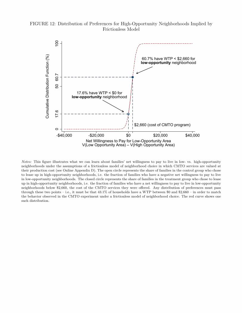
FIGURE 12: Distribution of Preferences for High-Opportunity Neighborhoods Implied byFrictionless Model

$2,660 (cost of CMTO program)

60.7% have WTP < $2,660 forlow-opportunity neighborhood

17.6% have WTP < $0 forlow-opportunity neighborhood

017

.650

60.7

100

Cum

ulat

ive

Dis

tribu

tion

Func

tion

(%)

-$40,000 -$20,000 $0 $20,000 $40,000Net Willingness to Pay for Low-Opportunity Area

V(Low Opportunity Area) – V(High Opportunity Area)

Notes: This figure illustrates what we can learn about families’ net willingness to pay to live in low- vs. high-opportunityneighborhoods under the assumptions of a frictionless model of neighborhood choice in which CMTO services are valued attheir production cost (see Online Appendix D). The open circle represents the share of families in the control group who choseto lease up in high-opportunity neighborhoods, i.e. the fraction of families who have a negative net willingness to pay to livein low-opportunity neighborhoods. The closed circle represents the share of families in the treatment group who chose to leaseup in high-opportunity neighborhoods, i.e. the fraction of families who have a net willingness to pay to live in low-opportunityneighborhoods below $2,660, the cost of the CMTO services they were offered. Any distribution of preferences must passthrough these two points – i.e., it must be that 43.1% of households have a WTP between $0 and $2,660 – in order to matchthe behavior observed in the CMTO experiment under a frictionless model of neighborhood choice. The red curve shows onesuch distribution.

FIGURE 13: Effects of Voucher Payment Standards on Moving to Opportunity:Quasi-Experimental Estimates

A. KCHA 5-Tier Payment Standard Reform

5 Tier Reformin KCHA

010

2030

4050

6070

Perc

ent o

f Hou

seho

lds

Who

Mov

edto

Hig

h O

ppor

tuni

ty A

reas

Aug/Sep2015

Oct/Nov2015

Dec/Jan2015/16

Feb/Mar2016

Apr/May2016

Jun/Jul2016

Aug/Sep2016

Oct/Nov2016

Date of Voucher IssuanceEffect of 5-Tier Reform: -3.59 ranks

(5.75)

KCHA

SHA

If voucher holders from KCHA had received CMTO treatment in March 2016

38 pp

B. SHA Family Access Supplement for High-Opportunity Areas

SupplementIntroduced

010

2030

4050

6070

80

Perc

ent o

f Hou

seho

lds

Who

Mov

edto

Hig

h O

ppor

tuni

ty A

reas

Aug/Sep2017

Oct/Nov2017

Dec/Jan2017/18

Feb/Mar/Apr2018

May/Jun2018

Jul/Aug2018

Sep/Oct2018

Date of Voucher Issuance

HHs w/ Kids

HHs w/out Kids

Effect of Family Access Supplement: 13.79 pp(5.11)

CMTO Pilot

Notes: This figure plots the share of households who move to high-opportunity areas around the introduction of two paymentstandard reforms, in two-month units. In Panel A, we analyze the introduction of a 5-Tier Voucher Payment Standard systemin March 2016 by the King County Housing Authority, which increased payment standards in more expensive neighborhoods.We plot the fraction of voucher recipients with children who choose to lease up in high-opportunity areas (as defined in theCMTO experiment in Figure 2) in both KCHA and SHA around this reform. We also report a difference-in-difference estimateof the treatment effect, estimated using the specification in Section VII.A. As a benchmark, we show the effect of the CMTOintervention on the same scale using the dashed line in the figure. This line is constructed by adding the treatment effect ofCMTO on moving to high-opportunity areas shown in Figure 4a to the grey series after March 2016. In Panel B, we analyzethe introduction of the Family Access Supplement (FAS) in SHA in February 2018, which increased payment standards inhigh-opportunity areas as defined exactly in the CMTO experiment. The FAS was implemented at the same time as the startof the CMTO pilot, which was conducted from Februrary-April 2018, shown by the shaded region in the figure, and continuedafter the pilot ended. The FAS was only available to families with children; we therefore use families without children withinSHA as a comparison group to evaluate the impacts of this reform. We again plot the fraction of voucher recipients in eachgroup who choose to lease up in high-opportunity areas around this reform and report a difference-in-difference estimate ofthe reform’s impact (excluding the CMTO pilot period) using the specification in Section VII.A.

APPENDIX FIGURE 1: Causal Effects of Moving to a Better Neighborhood by Age at Move:Evidence from Prior Research

A. United States

Source: Chetty, Friedman, Hendren, Jones, Porter (2018)

B. Australia

Source: Deutscher (2018)

C. Montreal, Canada

Source: Laliberté (2018)

E. MTO: Baltimore, Boston, Chicago, LA, NYC

Source: Chetty, Hendren, Katz (AER 2016)

F. Chicago Public Housing Demolitions

Source: Chyn (AER 2018)

D. Denmark

Source: Faurschou (2018)

Notes: This figure reproduces estimates from a recent set of papers estimating the the causal effects of the neighborhoodin which a child grows up on his or her outcomes in adulthood. Each panel depicts the causal effect of moving to an areawith better observed outcomes, by the age at which children make that move. Panels A-D all use variants of the moversresearch design developed in Chetty and Hendren (2018) to estimate childhood exposure effects. Panel A presents tract-levelestimates of exposure effects on income in the U.S. from Chetty, Friedman, Hendren, Jones and Porter (2018). Panel Bpresents estimates of exposure effects on income in Australia from Deutscher (2018). Panel C presents estimates of exposureeffects on university enrollment in Montreal, Canada from Laliberte (2018). Panel D presents exposure effect estimates onincome in Denmark from Faurschou (2018). Panel E shows treatment effects on income in adulthood by age at move fromthe Moving to Opportunity experiment studied in Chetty, Hendren and Katz (2016). Panel F shows Chyn’s (2018) estimatesof the effect of moving to a better neighborhood on income in adulthood by age at move, exploiting the demolition of publichousing projects as a quasi-experiment.

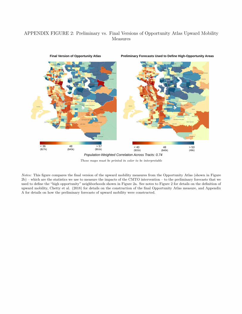
APPENDIX FIGURE 2: Preliminary vs. Final Versions of Opportunity Atlas Upward MobilityMeasures

Preliminary Forecasts Used to Define High-Opportunity AreasFinal Version of Opportunity Atlas

Population-Weighted Correlation Across Tracts: 0.74

> 57 ($51k)

48($40k)

< 36 ($27k)

> 53 (46k)

48($40k)

< 40($31k)

These maps must be printed in color to be interpretable

Notes: This figure compares the final version of the upward mobility measures from the Opportunity Atlas (shown in Figure2b) – which are the statistics we use to measure the impacts of the CMTO intervention – to the preliminary forecasts that weused to define the “high opportunity” neighborhoods shown in Figure 2a. See notes to Figure 2 for details on the definition ofupward mobility, Chetty et al. (2018) for details on the construction of the final Opportunity Atlas measure, and AppendixA for details on how the preliminary forecasts of upward mobility were constructed.

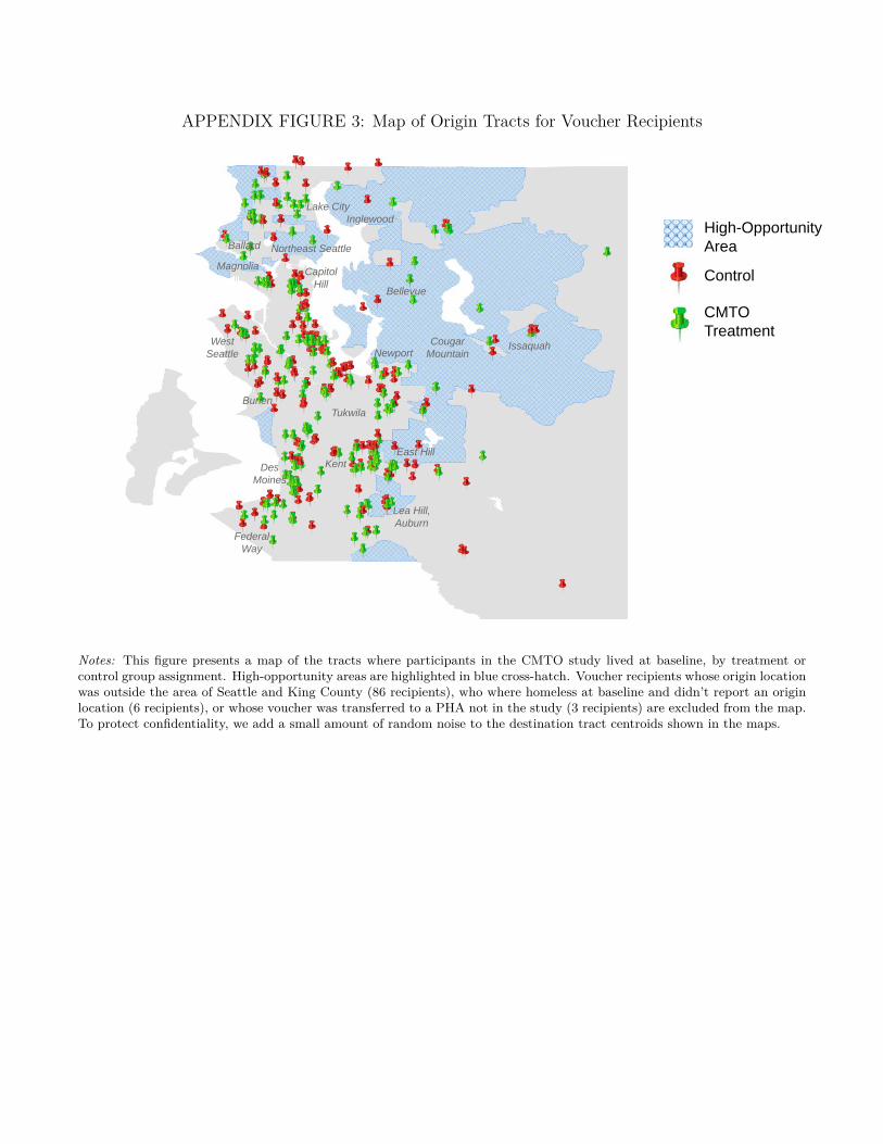
APPENDIX FIGURE 3: Map of Origin Tracts for Voucher Recipients

High-Opportunity Area

West Seattle

Des Moines

Magnolia

Northeast Seattle

NewportCougar

Mountain

Lea Hill, Auburn

East Hill

Inglewood

Issaquah

Lake City

Kent

TukwilaBurien

BellevueControl

CMTOTreatment

Federal Way

Capitol Hill

Ballard

Notes: This figure presents a map of the tracts where participants in the CMTO study lived at baseline, by treatment orcontrol group assignment. High-opportunity areas are highlighted in blue cross-hatch. Voucher recipients whose origin locationwas outside the area of Seattle and King County (86 recipients), who where homeless at baseline and didn’t report an originlocation (6 recipients), or whose voucher was transferred to a PHA not in the study (3 recipients) are excluded from the map.To protect confidentiality, we add a small amount of random noise to the destination tract centroids shown in the maps.

APPENDIX FIGURE 4: Predicted Treatment Effects on Other Long-Term Outcomes

A. Teenage Birth Rates of Children from Low-Income Families

21.1%

16.5%

010

2030

Mea

n Te

en B

irth

Rat

e W

hen

Pare

nts

at p

=25

in T

ract

(%)

Control TreatmentDifference: -4.6 pp SE: (0.8)

B. Incarceration Rates of Children from Low-Income Families

2.0%

1.6%

01

23

Mea

n In

carc

erat

ion

Rat

e W

hen

Pare

nts

at p

=25

in T

ract

(%)

Control TreatmentDifference: -0.4 pp SE: (0.1)

Notes: These figures replicate Panel D of Figure 4, plotting the predicted effects of CMTO on other long-term outcomes basedon the destination tract to which families moved. Importantly, as in Figure 4d, these are not outcomes of CMTO participantsthemselves. Rather, they are outcomes of children in the 1978-83 birth cohorts who grew up in households with family incomeat the 25th percentile of the national income distribution in the destination neighborhoods to which CMTO participantsmoved. Panel A presents the predicted effect on the tract-level teenage birth rates for women, drawing on data from theOpportunity Atlas. Panel B presents the predicted effect on incarceration rates (on April 1, 2010) for children who grew upin the tract. We construct these in exactly the same way as Panel D of Figure 4, simply changing the outcome variable; seenotes to that figure for details.

APPENDIX FIGURE 5: Unconditional Short-Run Persistence of Treatment Effects onNeighborhood Choice

16.9%

56.9%

16.9%

55.8%

020

4060

Perc

enta

ge o

f Hou

seho

lds

who

Liv

ein

a H

igh

Opp

ortu

nity

Are

a

Feb 6, 2019 Feb 6, 2020 Feb 6, 2019 Feb 6, 2020

ControlTreatment

Change in Treatment Effect from Feb 6, 2019 to 2020: -1.1 pp SE: (11.9)

Notes: This figure replicates Panel A of Figure 9, but does not condition on families leasing up a unit. See notes to that figurefor details.

APPENDIX FIGURE 6: Treatment Effects on Post-Move Neighborhood Satisfaction

A. Satisfaction with New Neighborhood

0.0%3.0% 3.0%

21.2%

27.3%

45.5%

2.1% 2.1%

7.2%

13.4% 12.4%

62.9%

n = 0n = 1 n = 1

n = 7

n = 9

n = 15

n = 2 n = 2

n = 7

n = 13 n = 12

n = 61

020

4060

Nei

ghbo

rhoo

d Sa

tisfa

ctio

n

NoAnswer

VeryDissatisfied

SomewhatDissatisfied

NeitherSatisfied norUnsatisfied

SomewhatSatisfied

VerySatisfied

ControlTreatment

Difference in % Very Satisfied: 17.3pp SE: (10.1)

B. Certainty about Wanting to Stay in New Neighborhood

0.0%

24.2%

12.1% 12.1%

21.2%

30.3%

2.1%6.2%

12.4%16.5% 16.5%

46.4%

n = 0

n = 8

n = 4 n = 4

n = 7

n = 10

n = 2

n = 6

n = 12

n = 16 n = 16

n = 45

020

4060

Cer

tain

ty A

bout

Wan

ting

to S

tay

or L

eave

NoAnswer

Very SureWants to

Move

SomewhatSure

Wants toMove

In the Middle SomewhatSure

Wants toStay

Very SureWants to

Stay

ControlTreatment

Difference in % Very Sure Want to Stay: 16.3pp SE: (9.7)

Notes: This figure uses data from a follow-up qualitative survey administered to a random sample of CMTO participants.Panel A shows the distribution of neighborhood satisfaction in the treatment and control groups. Participants were asked,“Which of the following statements best describes how satisfied you are with your current neighborhood? 1. Very Satisfied -2. Somewhat satisfied - 3. In the middle - 4. Somewhat dissatisfied - 5. Very dissatisfied - 6. (No Answer).” Panel B presentsmeasures of the certainty with which participants want to stay in their new neighborhood. Participants were asked, “Whichof the following statements best describes how you feel about staying in your current neighborhood? - 1. Very sure I want tostay - 2. Somewhat sure I want to stay - 3. In the middle - 4. Somewhat sure I want to move to a different neighborhood - 5.Very sure I want to move to a different neighborhood - 6. (No Answer).” The sample consists of all households who leased-upand were surveyed after lease-up.

APPENDIX FIGURE 7: Changes to King County Housing Authority Payment Standards inMarch 2016

> $400

$250

< $150

Increase in Max Rent

for 2BR Apt.

Notes: This figure maps the changes in payment standards implemented in March 2016 by KCHA. The map plots the changesin the maximum monthly rent for a two-bedroom apartment that could be paid for using a housing voucher from KCHA,comparing maximum rents in the pre-period (January 2015 to February 2016) to the post-period (March 2016 to December2017). Darker areas experienced larger increases in maximum rent allowances.