
Creating a Pseudo-CT from MRI for MRI-only based …€¦ · This is due to the fact that MRI...
101
-
Upload
phungkhanh -
Category
Documents
-
view
214 -
download
0
Transcript of Creating a Pseudo-CT from MRI for MRI-only based …€¦ · This is due to the fact that MRI...

Creating a Pseudo-CT from MRIfor MRI-only based Radiation
Therapy Planning
Daniel Andreasen
Kongens Lyngby 2013
IMM-MSc-2013-10

Technical University of Denmark
Informatics and Mathematical Modelling
Building 321, DK-2800 Kongens Lyngby, Denmark
Phone +45 45253351, Fax +45 45882673
www.imm.dtu.dk IMM-MSc-2013-10

Summary (English)
Background: In the planning process of external radiation therapy, CT is usedas the main imaging modality. The advantage of using CT is that the voxelintensity values are directly related to electron density which is needed for dosecalculations. Furthermore, CT provides an accurate geometrical representationof bone needed for constructing digitally reconstructed radiographs. In recentyears, interest in replacing CT with MRI in the treatment planning processhas emerged. This is due to the fact that MRI provides a superior soft tissuecontrast; a desirable property that could increase the accuracy of target andrisk volume delineation. The challenge in replacing CT with MRI is that theMRI intensity values are not related to electron densities and conventional MRIsequences cannot obtain signal from bone.
The purpose of this project was to investigate the use of Gaussian MixtureRegression (GMR) and Random Forest regression (RaFR) for creating a pseudo-CT image from MRI images. Creating a pseudo-CT from MRI would eliminatethe need for a real CT scan and thus facilitate an MRI-only work �ow in theradiation therapy planning process. The use of GMR for pseudo-CT creation haspreviously been reported so the reproducibility of these results was investigated.dUTE and mDixon MRI image sets as well as Local Binary Pattern (LBP)feature images were investigated as input to the regression models.
Materials and methods: Head scans of three patients �xated for whole brainradiation therapy were acquired on a 1 T open MRI scanner with �ex coils.dUTE and mDixon image sets were obtained. CT head scans were also acquiredusing a standard protocol. A registration of the CT and MRI image sets wascarried out and LBP feature images were derived from the dUTE image sets.

ii
All RaFR and GMR models were trained with the dUTE image sets as basicinput. Some of the models were trained with an additional mDixon or LBPinput in order to investigate if these inputs could improve the quality of thepredicted pseudo-CT. More speci�cally, the impact of adding the LBP inputwas investigated using RaFR and the impact of adding an mDixon input wasinvestigated using both RaFR and GMR. A study of the optimal tree depthfor RaFR was also carried out. The quality of the resulting pseudo-CTs wasquanti�ed in terms of the prediction deviation, the geometrical accuracy of boneand the dosimetric accuracy.
Results: In the LBP input study, the results indicated that using LBPs couldimprove the quality of the pseudo-CT.
In the mDixon input study, the results suggested that both RaFR and GMRmodels were improved when adding the mDixon input. The improvement wasmainly observed in terms of smaller prediction deviations in the bone region ofthe pseudo-CTs and a greater geometrical accuracy. When comparing RaFRand GMR, it was found that using RaFR produced pseudo-CTs with the small-est prediction deviations and greatest geometrical accuracy. In terms of thedosimetric accuracy, the di�erence was less clear.
Conclusion: The use of GMR and RaFR for creating a pseudo-CT imagefrom MRI images was investigated. The reproducibility of previously reportedresults using GMR was demonstrated. Furthermore, the impact of adding LBPand mDixon inputs to the regression models was demonstrated and showed thatan improvement of the pseudo-CT could be obtained. The results serves as amotivation for further studies using more data and improved feature images.

Summary (Danish)
Baggrund: I planlægningen af ekstern stråleterapi anvendes CT som den pri-mære skanningsmodalitet. Fordelen ved at anvende CT er, at voxel-intensitetsværdierer direkte relateret til elektrontætheden af vævet, der afbildes. Dette er nød-vendigt for at kunne udføre dosisberegninger. Desuden giver CT en nøjagtiggeometrisk repræsentation af knogle, som er nødvendig for at generere digitaltrekonstruerede røntgenbilleder a�edt fra CT. I de seneste år er interessen for aterstatte CT med MRI i planlægningsprocessen opstået. Dette skyldes det fak-tum, at MRI er CT overlegen, når det kommer til bløddelskontrast; en vigtigegenskab, der kan øge indtegningsnøjagtigheden af tumorvolumener og risiko-organer. Udfordringen i at erstatte CT med MRI er, at MRI intensitetsværdierikke er direkte relateret til elektrontæthed samt at konventionelle MRI sekvenserikke kan opnå signal fra knogle.
Formålet med dette projekt var at undersøge brugen af Gaussian Mixture Re-gression (GMR) og Random Forest regression (RaFR) for at skabe et pseudo-CTbillede ud fra MRI-billeder. Dannelsen af et pseudo-CT fra MRI kan potentielteliminere behovet for en CT-scanning og dermed muliggøre et work �ow base-ret udelukkende på MRI. Anvendelsen af GMR til at generere pseudo-CTer ertidligere blevet rapporteret, så et mål med projektet var at undersøge repro-ducerbarheden af resultaterne. dUTE og mDixon MRI skanninger samt LocalBinary Pattern (LBP) featurebilleder blev undersøgt som input til regressions-modellerne.
Materialer og metoder: Tre patienter som skulle modtage helhjerne stråle-behandling blev skannet på en 1 T åben MRI-skanner med �ex-spoler. dUTE ogmDixon billedsæt blev optaget. En CT skanning af hovedet blev også optaget

iv
ved hjælp af standardprotokol. CT- og MRI-billedsæt blev indbyrdes registre-ret og LBP featurebilleder blev a�edt fra dUTE billedsættene. Alle RaFR ogGMR modeller blev trænet med dUTE billedsæt som grundlæggende input.Nogle af modellerne blev trænet med et yderligere mDixon eller LBP input medhenblik på at undersøge om disse billedsæt kunne forbedre kvaliteten af pseudo-CTerne. Speci�kt blev virkningen af at tilføje LBP input undersøgt for RaFRog virkningen af at tilføje mDixon input undersøgt for både RaFR og GMR. Enundersøgelse af den optimale tree depth for RaFR blev også udført. Kvaliteten afde resulterende pseudo-CTs blev kvanti�ceret ved hjælp af den gennemsnitligeafvigelse mellem pseudo-CT og reference CT, den geometriske nøjagtighed afknogle i pseudo-CTet samt den dosimetriske nøjagtighed når pseudo-CTet blevbrugt til at beregne dosefordelinger.
Resultater: I undersøgelsen af LBP input viste resultaterne, at anvendelsen afLBP kunne forbedre kvaliteten af pseudo-CTet.
I undersøgelsen af mDixon input viste resultaterne, at både RaFR og GMRmodellerne blev forbedret ved brug af mDixon input. Forbedringerne gav sighovedsagligt til udtryk i mindre afvigelser i knogleregionen af pseudo-CTernesamt ved større geometrisk nøjagtighed. Ved sammenligning af RaFR og GMRfandtes det, at pseudo-CTer genereret med RaFR havde de mindste gennem-snitlige afvigelser samt største geometriske nøjagtighed. Med hensyn til dendosimetriske nøjagtighed var forskellen mellem GMR og RaFR ikke tydelig.
Konklusion: Anvendelsen af GMR og RaFR for at generere pseudo-CT-billederfra MRI-billeder blev undersøgt. Reproducerbarheden af tidligere rapporterederesultater ved anvendelse af GMR blev demonstreret. Endvidere blev virkningenaf at tilføje LBP og mDixon input til regressionsmodellerne undersøgt. Det blevvist, at en forbedring af pseudo-CTet derved kunne opnås. Resultaterne tjenersom en motivation for at udføre yderligere undersøgelser med mere data ogforbedrede featurebilleder.

Preface
This thesis was prepared at the department of Informatics and MathematicalModelling at the Technical University of Denmark and at the department ofOncology at Copenhagen University Hospital, Herlev. The work corresponds to30 ECTS points and it was done in partial ful�lment of the requirements foracquiring an M.Sc. in Medicine and Technology at the Technical University ofDenmark and the University of Copenhagen.
SupervisorsJens M. Edmund, Ph.D., DABRDepartment of Oncology (R)Copenhagen University Hospital, Herlev
Koen Van Leemput, Ph.D.Department of Informatics and Mathematical ModellingTechnical University of Denmark
Lyngby, 01-March-2013
Daniel Andreasen

vi

Acknowledgements
First of all, I would like to thank the Department of Oncology at Herlev Hospitalfor making this project possible and allowing me to work in an exciting clinicalenvironment. It has given me great insight and I have felt very privileged. Iwould like to thank Rasmus H. Hansen, who set up the MRI scanner for thespecial sequences used in my project, and Jon Andersen, who was in charge ofrecruiting patients. Without their help, much of this project would not havebeen possible.
Also, a great thanks to both of my supervisors, Jens M. Edmund and Koen VanLeemput for their guidance, enthusiasm and great help with this project.
Finally, I would like to thank my friends and family for their support and feed-back throughout the project. A special thanks to my girlfriend, Minna, whosesupport and faith in me has been invaluable in stressful times.

viii

Acronyms and symbols
Acronyms
CART Classi�cation and Regression TreeCNR Contrast-to-Noise RatioCT Computed Tomography
DRR Digitally Reconstructed RadiographdUTE di�erence UTE (dual echo UTE)DVH Dose-Volume Histogram
EM Expectation Maximization
FOV Field of View
GMM Gaussian Mixture ModelGMR Gaussian Mixture RegressionGTV Gross Tumour VolumeGy gray
HU Houns�eld unit
ICRU The International Commission on RadiationUnits & Measurements
LBP Local Binary PatternLINAC Linear accelerator

x Acronyms
MAPD Mean Absolute Prediction DeviationmDixon multi-echo DixonMPD Mean Prediction DeviationMRI Magnetic Resonance ImagingMSPD Mean Squared Prediction DeviationMU Monitor Unit - a standardized measure of ma-
chine output for a LINAC
OR Organ at Risk
pCT pseudo-CTpdf Probability Density FunctionPET Positron Emission TomographyPRV Planning Risk VolumePTV Planning Target Volume
RaF Random ForestRaFR Random Forest RegressionRF Radio FrequencyRT Radiation Therapy
SNR Signal-to-Noise Ratiostd Standard Deviation
T Tesla
UTE Ultra Short Echo Time

xi
List of symbols
α Flip angleβ Split parameters of a node in a decision treedTE Time interval between echo acquisitions in the
multi-echo Dixon sequenceF Magnitude of the magnetization of fatφ Multivariate Gaussian Probability density func-
tionπj Prior weight in a Gaussian Mixture ModelT1 Longitudinal magnetization relaxation time
constantT2 Transversal magnetization relaxation time con-
stantT ∗2 Time constant of the free induction decayTAQ Acquisition timeTE Echo timeΘ Phase angleθ Parameters of a Gaussian Mixture Modelϕ Error phase due to �eld inhomogeneitiesϕ0 Error phase due to MRI system �awsW Magnitude of the magnetization of water

xii

Contents
Summary (English) i
Summary (Danish) iii
Preface v
Acknowledgements vii
Acronyms and symbols ixAcronyms . . . . . . . . . . . . . . . . . . . . . . . . . . . . . . . . . . ixList of symbols . . . . . . . . . . . . . . . . . . . . . . . . . . . . . . . xi
1 Introduction and Background 11.1 MRI-only Radiation Therapy Planning . . . . . . . . . . . . . . . 2
1.1.1 dUTE Imaging . . . . . . . . . . . . . . . . . . . . . . . . 21.1.2 Dixon Imaging . . . . . . . . . . . . . . . . . . . . . . . . 31.1.3 Estimating CT from MRI . . . . . . . . . . . . . . . . . . 3
1.2 Random Forest Regression . . . . . . . . . . . . . . . . . . . . . . 41.3 Objectives . . . . . . . . . . . . . . . . . . . . . . . . . . . . . . . 5
2 Theory 72.1 dUTE MRI Sequence . . . . . . . . . . . . . . . . . . . . . . . . . 7
2.1.1 Parameters . . . . . . . . . . . . . . . . . . . . . . . . . . 82.1.2 dUTE Artefacts . . . . . . . . . . . . . . . . . . . . . . . 9
2.2 Dixon MRI Sequence . . . . . . . . . . . . . . . . . . . . . . . . . 112.3 Registration Method . . . . . . . . . . . . . . . . . . . . . . . . . 132.4 Gaussian Mixture Regression . . . . . . . . . . . . . . . . . . . . 15
2.4.1 Gaussian Mixture Model . . . . . . . . . . . . . . . . . . . 152.4.2 Regression using a Gaussian Mixture Model . . . . . . . . 16

xiv CONTENTS
2.4.3 Impact of Changing the Number of Components . . . . . 18
2.5 Random Forest Regression . . . . . . . . . . . . . . . . . . . . . . 20
2.5.1 Decision Trees . . . . . . . . . . . . . . . . . . . . . . . . 20
2.5.2 Random Forests . . . . . . . . . . . . . . . . . . . . . . . 22
2.5.3 E�ect of Forest Size . . . . . . . . . . . . . . . . . . . . . 23
2.5.4 E�ect of Tree Depth . . . . . . . . . . . . . . . . . . . . . 24
2.6 Local Binary Pattern Feature Representation . . . . . . . . . . . 25
2.7 Evaluation of Results . . . . . . . . . . . . . . . . . . . . . . . . . 27
2.7.1 Prediction Deviation . . . . . . . . . . . . . . . . . . . . . 27
2.7.2 Geometric Evaluation . . . . . . . . . . . . . . . . . . . . 28
2.7.3 Dosimetric Evaluation . . . . . . . . . . . . . . . . . . . . 28
3 Methods and Procedures 31
3.1 Data Acquisition and Preprocessing . . . . . . . . . . . . . . . . 31
3.1.1 Scanner Set-up . . . . . . . . . . . . . . . . . . . . . . . . 31
3.1.2 Registration . . . . . . . . . . . . . . . . . . . . . . . . . . 32
3.1.3 Local Binary Pattern-like Feature Extraction . . . . . . . 32
3.1.4 Filtering . . . . . . . . . . . . . . . . . . . . . . . . . . . . 33
3.1.5 Air Mask . . . . . . . . . . . . . . . . . . . . . . . . . . . 34
3.1.6 De�ning the Input/Output Data for the Models . . . . . 35
3.2 Gaussian Mixture Regression . . . . . . . . . . . . . . . . . . . . 35
3.2.1 mDixon Input Study . . . . . . . . . . . . . . . . . . . . . 36
3.3 Random Forest Regression . . . . . . . . . . . . . . . . . . . . . . 36
3.3.1 Model Optimization Study . . . . . . . . . . . . . . . . . 36
3.3.2 LBP Input Study . . . . . . . . . . . . . . . . . . . . . . . 37
3.3.3 mDixon Input Study . . . . . . . . . . . . . . . . . . . . . 37
3.4 Post-processing . . . . . . . . . . . . . . . . . . . . . . . . . . . . 37
3.4.1 Prediction Deviation . . . . . . . . . . . . . . . . . . . . . 37
3.4.2 Geometric Evaluation . . . . . . . . . . . . . . . . . . . . 38
3.4.3 Dose Plan and DVHs . . . . . . . . . . . . . . . . . . . . 38
4 Results 39
4.1 Random Forest Model Optimization . . . . . . . . . . . . . . . . 39
4.2 Random Forest LBP Input . . . . . . . . . . . . . . . . . . . . . 41
4.3 mDixon Input Study . . . . . . . . . . . . . . . . . . . . . . . . . 42
4.3.1 Prediction Deviations . . . . . . . . . . . . . . . . . . . . 42
4.3.2 Geometric Evaluation . . . . . . . . . . . . . . . . . . . . 44
4.3.3 Dosimetric Evaluation . . . . . . . . . . . . . . . . . . . . 46
4.3.4 Comparing GMR and RaF . . . . . . . . . . . . . . . . . 49

CONTENTS xv
5 Discussion 535.1 Random Forest Model Optimization Study . . . . . . . . . . . . 535.2 Random Forest Local Binary Pattern Input Study . . . . . . . . 545.3 mDixon Input Study . . . . . . . . . . . . . . . . . . . . . . . . . 56
5.3.1 Gaussian Mixture Regression . . . . . . . . . . . . . . . . 565.3.2 Random Forest Regression . . . . . . . . . . . . . . . . . 585.3.3 Comparing GMR and RaFR . . . . . . . . . . . . . . . . 585.3.4 General Comments on the pCTs . . . . . . . . . . . . . . 60
5.4 Evaluation Methods . . . . . . . . . . . . . . . . . . . . . . . . . 615.4.1 Prediction Deviation Method . . . . . . . . . . . . . . . . 615.4.2 Geometric Evaluation Method . . . . . . . . . . . . . . . 615.4.3 Dosimetric Evaluation Method . . . . . . . . . . . . . . . 62
5.5 Future Work . . . . . . . . . . . . . . . . . . . . . . . . . . . . . 62
6 Conclusion 65
A Abstract Accepted for ESTRO Forum 2013 69
Bibliography 79

xvi CONTENTS

Chapter 1
Introduction andBackground
Despite the growing interest in using magnetic resonance imaging (MRI) in theplanning process of external radiation therapy (RT), Computed Tomography(CT) remains the golden standard. This is due to the fact that a planning CTscan provides electron density information which is critical to the calculation ofthe 3D dose distribution in the irradiated tissues. Furthermore, the CT providesan accurate geometrical representation of bone, which is needed for constructinga digitally reconstructed radiograph (DRR); a 2D planar reference image createdfrom the CT image set. This is used in combination with traditional X-rayimages taken at the linear accelerator (LINAC) to verify proper patient setupwith respect to the isocenter of the LINAC [1].
In conventional external RT planning, CT is the only imaging modality used. Aconsequence of this is that delineation of e.g. the tumour volume and potentialorgans at risk (ORs) must be done on the CT image sets. In 2006, Khoo andJoon outlined the advantages of introducing MRI in the planning process [2].Their main point was that MRI contributes with an increased soft tissue con-trast, yielding a better characterization of tissues, which in CT appear verysimilar. Kristensen et al. later showed that delineating structures on MRI im-ages leads to more accurate volume de�nitions [3]. For this reason, an MRI/CTwork �ow has become common practice at Herlev Hospital where structures are

2 Introduction and Background
delineated on MRI image sets and then transferred to the CT image sets fordose plan calculation. The transfer of delineations is carried out using a rigidregistration between the MRI and CT image sets.
Aside from requiring an extra scan of the patient, the MRI/CT work �ow hassome disadvantages. Nyholm et al. estimated that systematic spatial uncertain-ties of 2 mm are introduced with the rigid registration between MRI and CT [4].The term systematic refers to the fact that the same error is repeated over andover, as opposed to the random errors introduced with e.g. a less than perfectpatient alignment with respect to the LINAC. The systematic errors may inother words cause a constant partial miss of the tumour volume and potentiallyresult in an increased dose to organs at risk (ORs).
1.1 MRI-only Radiation Therapy Planning
With the advances of MRI in RT treatment planning and with the introduc-tion of PET/MRI systems, the interest and research in entirely replacing CTwith MRI has increased [5�7]. This would eliminate the registration inducedsystematic errors and reduce the amount of scanning sessions needed. The ap-proach has been to generate an estimate of CT images from MRI images, a socalled pseudo-CT (pCT) which could then be used for dose calculation in RTtreatment planning and for attenuation correction in PET/MRI. The challengeis that there is no direct relation between MRI intensity and electron density.Furthermore, conventional MRI cannot depict cortical bone very well becausethe bone signal is lost before the readout begins. This is due to the short T2 ofcortical bone.
1.1.1 dUTE Imaging
In 2003, Robson et al. described the basic ultra short echo time (UTE) MRIsequence and its ability to acquire signal from bone and ligaments [8]. Theso-called di�erence UTE (dUTE) sequence was also introduced as a means ofenhancing the visibility of short T2 components. This was achieved by acquir-ing a gradient echo shortly after the �rst acquisition and then subtracting thetwo image sets to isolate the short T2 components. Several authors have laterused the dUTE sequence for pCT estimation or attenuation correction [5,9�11].At Herlev Hospital, Kjer investigated the dUTE sequence and found optimalacquisition parameters for the 1 Tesla (T) open MRI scanner on site [12]. With

1.1 MRI-only Radiation Therapy Planning 3
regard to these parameters, it should be noted that at the stated optimal sec-ond echo time of the dUTE, phase cancellation artefacts may occur due to thechemical shift between water and fat. This in turn may cause non-bone tissueto appear as bone (see Section 2.1 for more details).
1.1.2 Dixon Imaging
In the �eld of PET/MRI some of the same challenges are present as in MRI-onlyRT treatment planning. Here, attenuation maps for attenuation correction needto be derived. This was previously obtained from CT using its direct correlationwith electron density. Because it has been found important to account foradipose tissue in whole-body MRI-based attenuation correction, the Dixon MRIsequence has been investigated for its possible use in generating attenuationmaps [9,13,14]. This sequence provides water-only and fat-only image sets andfor this reason is appropriate for segmenting water and fat in MRI images.
1.1.3 Estimating CT from MRI
Di�erent approaches have been used to generate pCTs. One is an atlas-basedestimation. With this method, an atlas of many co-registered MRI and CTimage sets is made. To estimate a pCT for a new patient, the MRI atlas canbe deformed to �t the new patient's MRI. The same deformation can thenbe applied to the CT atlas to obtain an estimate of the pCT. A variation ofthe standard atlas-based method was done by Hofmann et al. [15]. They usedpatches in T1 weighted images and the spatial position from an atlas as featuresto train a regression model used to predict the pCT. The fact that no specialMRI sequences, such as the dUTE, was needed to generate the pCT seems to bethe main strength of this atlas-based method. In general however, atlas-basedmethods are known to su�er from inaccuracies when the inter-patient variabilityis large [16].
Another approach has been to do a voxel-wise segmentation of the MRI. Herea characterization of each voxel in the MRI is done in order estimate a pCT.A common characteristic of the voxel-wise methods seems to be the need forspecial MRI sequences like the dUTE or Dixon in order to compensate for thepreviously mentioned shortcomings of conventional MRI.In the �eld of PET/MRI Martinez-Möller et al. used thresholds to segmentDixon MRI images into air/lung/fat/soft tissue classes which were then assigned
4 Introduction and Background
bulk attenuation factors. They did not take bone into account [13]. Berker etal. used a combined dUTE/Dixon sequence to obtain an air/bone/fat/soft tis-sue segmentation, again using thresholds [9]. Both Martinez-Möller et al. andBerker et al. reported improvements in segmentation accuracy when using theDixon sequence. They quanti�ed the accuracy of their methods by looking atthe agreement with CT attenuation correction and not at the similarity betweenthe pCT and real CT, which makes it hard to compare their method with others'.
Instead of segmenting the MRI images into di�erent tissue classes, Johanssonet al. tried to predict the CT image by using a Gaussian mixture regression(GMR) method. Data was collected from 5 patients who were CT scanned (oneimage set) and MRI scanned on a 1.5 T scanner with two dUTE sequences atdi�erent �ip angles and one T2 weighted sequence (5 image sets in total). Eachof the 5 MRI image sets were �ltered using a mean �lter and a standard devia-tion (std) �lter to create 10 more image sets (5 mean �ltered and 5 std �ltered).An air mask was used to reduce the data amount and the regression model wasthen estimated using k-means and expectation maximization (EM) algorithmsto estimate the mixing proportions, mean values and covariance matrices. ThepCT was compared to the actual CT image using the mean absolute predictiondeviation (MAPD) inside the air mask. It was found to be 137 HU on averagefor all �ve patients with a variation from 117 to 176 HU for individual patients.The method showed very promising results and was able to distinguish bonefrom air. The largest di�erences between pCT and CT were seen at bone/tissueand air/tissue interfaces (paranasal sinuses). This was attributed to suscepti-bility e�ects causing a very short T ∗2 . In a later publication, Johansson et al.
explored the voxel-wise uncertainty of the model and used the mean predictiondeviation (MPD) and MAPD to determine if model reduction was possible [16].Here, they found that the T2 weighted image set was redundant in their model.
1.2 Random Forest Regression
Random Forest regression (RaFR) has to the knowledge of the author not beenused for predicting pCTs from MRI prior to this project. However, it has beenused to predict organ bounding boxes in both MRI Dixon and CT image setswith promising results [17,18]. To predict organ bounding boxes in Dixon MRIimage sets, Pauly et al. used a local binary pattern-like feature in order todescribe each pixel by its neighbourhood appearance [17]. The regression taskwas a bit di�erent from that of predicting a pCT since they were not trying topredict a CT value but a distance to a bounding box for every MRI voxel.

1.3 Objectives 5
1.3 Objectives
Inspired by the approach of Johansson et al., a regression approach was takenon in this project in order to �nd a mapping of MRI intensity values into CTdensities. More speci�cally, the Gaussian mixture regression model was usedin order to test its robustness and the reproducibility of results in a di�erentclinical set up. Motivated by the promising results of Pauly et al. RandomForest regression was studied as a method for predicting pCTs. Also, the use ofLocal Binary Pattern (LBP) as input to RaFR was studied.
Building on the prior experiences with voxel-wise methods, it was expected thatspecial MRI sequences would be needed to generate a pCT. For this reasonthe dUTE acquisition method was adopted. The data was collected using thescanner-speci�c dUTE acquisition parameters reported by Kjer. From the modelreduction study by Johansson et al., the method of using two di�erent �ip anglesfor the dUTE and adding �ltered images to the regression models showed toimprove the prediction accuracy. These methods were also adopted.
As mentioned, phase cancellation artefacts in water/fat containing voxels weresuspected to be present in the dUTE image sets; an issue speci�c for the 1 Tscanner at Herlev Hospital. Based on the experience that the Dixon sequencecan help in distinguishing water and fat it was investigated whether the sequencecould improve the regression models used.
With this established, the main objectives of the project can be summarized asfollows:
1. Investigate the use of Gaussian mixture regression for pCT generation.
2. Investigate the use of RaFR for pCT generation. This includes looking intooptimizing the model parameters and using a Local Binary Pattern-likefeature.
3. Investigate the impact of using a Dixon sequence in both models.
4. Compare the performance of Gaussian mixture regression versus that ofRandom Forest regression for pCT generation.
5. Quantify the di�erences between the reference CT and the pCT in mea-sures relevant for radiation therapy.

6 Introduction and Background

Chapter 2
Theory
2.1 dUTE MRI Sequence
Conventional MRI sequences are able to begin the readout of signal at a min-imum TE of about 8-10 ms [8]. This makes them inappropriate for detectionof signal from tissues that lose their transversal magnetization faster than this.Tissues such as cortical bone, periosteum and ligaments which have a T2 in therange 0.05-10 ms thus appear with a similar intensity as air in conventional MRIimages.
The ultra short echo time (UTE) MRI pulse sequence is optimized to detect sig-nal from tissues with a short T2. This means that an unconventional acquisitionapproach has been taken in order to minimize the time from excitation to read-out and to maximize the amount of signal coming from short T2 components inthis time frame. Because the image acquired with a UTE sequence shows highsignal intensities from both tissues with a short and a long T2, it is common torecord a second (or dual) echo shortly after the �rst. This technique is referredto as the di�erence UTE (dUTE) technique. In the resultant second image setthe tissues with short T2 will have lost a signi�cant amount of signal comparedto the long T2 tissues. The second image can thus be subtracted from the �rstto identify/isolate the short T2 components (see Figure 2.1).

8 Theory
Figure 2.1: Dual echo UTE images. Left: Image acquired at TE = 0.09 ms.Right: Image acquired at TE = 3.5 ms. As can be seen signalhas been lost from short T2 components in the second echo image.
Below, the UTE deviations from conventional MRI sequences will be outlined.It should be noted that these parameter deviations are related to the acquisitionof the �rst echo of the dUTE sequence, since this is recorded with an ultra shortecho time. The second echo is a conventional gradient echo.
2.1.1 Parameters
In general, 3 parameters are important when acquiring signal from short T2 com-ponents. These are the RF pulse duration, the echo time TE and the acquisitiontime TAQ.
RF pulse duration. In conventional MRI imaging the duration of the ex-citation RF pulse is not a concern since the T2 of the tissues being imaged islonger than the pulse duration. However, when dealing with tissues with a shortT2, loss of signal during the RF pulse becomes a problem [19]. To maximizethe transversal component of the magnetization in short T2 components, shortRF pulses are used which ensures the least amount of T2 relaxation during ex-citation. A consequence of this is that the �ip angle becomes lower than theconventional 90◦ (typically 40-70◦ less). It is important to note, that this lower�ip angle actually produces more signal from short T2 components, contrary towhat one might intuitively think.In a 3D UTE sequence a single RF pulse of short duration is used, where after3D radial readout gradients are used to traverse k-space.

2.1 dUTE MRI Sequence 9
Echo time. To get the most amount of signal from short T2 components theoptimal TE would ideally be 0 ms. This is not possible because the MRI coilsused for both excitation and signal acquisition need a little time to switch fromtransmit to receive mode. This is a physical limitation that depends on thescanner hardware used and in practice the shortest possible TE is used.
Acquisition time. With conventional MRI sequences k-space is traversed in alinear rectangular manner. To save time, sampling in UTE imaging is done in anon-linear fashion and simultaneous with the ramp up of the readout gradient,which leads to a radial (or centre-out) sampling. This in turn means that k-spacebecomes oversampled close to the centre and thus low spatial frequencies havea higher signal-to-noise ratio (SNR) than high ones [19]. TAQ is the samplingduration and this must be short enough for the short T2 tissues to not losesignal before the end of acquisition. On the other hand, some time is needed totraverse a certain distance from the centre of k-space in order to capture highspatial frequency components. In practice, a compromise must be made thatmaximizes signal and minimizes blurring, which means a TAQ of approximatelythe T2 of the tissue being imaged [19].
2.1.2 dUTE Artefacts
Because of the ultra short echo time, it is actually the free induction decay thatis measured during the readout of the �rst echo (which is thus not an echo inthe traditional sense). This means that it is impossible to distinguish betweenrelaxation due to T2 e�ects and relaxation due to T ∗2 e�ects. However, for fastrelaxing components, it is reasonable to assume that T2 ≈ T ∗2 [20]. This maynot hold at tissue interfaces where susceptibility e�ects cause de-phasing withinvoxels due to �eld inhomogeneities. This yields signal intensity artefacts becausetissue with an otherwise long T2 loses signal rapidly due to a short T ∗2 inducedby the �eld inhomogeneity.
Concerning the second echo acquisition, another artefact worth noting is thechemical shift or phase cancellation artefact. Because hydrogen bound in waterhas a slightly di�erent resonance frequency than that of hydrogen in fat, thesignal from these will at certain times after excitation periodically be in or outof phase. At out of phase times, less or no signal will be present in voxelscontaining a mixture of water and fat. Since the phase cancellation is timedependent, the severity of the artefact depends on the chosen TE . The chemicalshift (or di�erence in resonance frequencies) is measured in parts per million(ppm) and for water and fat it is 3.4 ppm. At 1 T, water has a resonancefrequency of 42 MHz, which in turn means that water and fat will be in phaseat a frequency of 3.4 ppm · 42 MHz = 142.8 Hz. This corresponds to every

10 Theory
7 ms. The �rst time after excitation when water and fat are out of phase isthus 3.5 ms. As mentioned, Kjer previously investigated the optimal acquisitionparameters for the dUTE sequence at the MRI scanner at Herlev Hospital. Hefound that a TE of 3.5 ms was close to the optimal echo time for the second echoin the dUTE sequence in terms of contrast-to-noise ratio (CNR) of the dUTEimage sets [12]. The dUTE image sets recorded on the 1 T scanner are thussusceptible to phase cancellation artefacts.

2.2 Dixon MRI Sequence 11
2.2 Dixon MRI Sequence
The Dixon technique was invented by W.T. Dixon in 1984 [21]. In short, thetechnique facilitates separating the signal originating from water and fat in MRIimages, which makes it possible to make water-only and fat-only images. Therationale is that, in many standard MRI sequences, fat appears hyper-intense,thus covering signal from other contents. This means that water-containingstructures of interest or contrast agents may be hard to discern in high-fatregions [22]. Also, the chemical shift artefact between water and fat may causephase cancellation or spatial shifts which is undesirable.In its original form, the Dixon technique is relatively simple. It is based on therecording of two images, one where water and fat are in phase (Θ = 0◦) andone were they are 180◦ out-of-phase (Θ = 180◦), a so-called 2-point method(because of the number of images recorded). By representing the MRI data asa complex signal it can be described using its magnitude and phase. If it isassumed that the imaged object only consists of water and fat, the signal canbe described as [23]:
S(x, y) = [W (x, y) + F (x, y) · eiΘ] · eiϕ(x,y) · eiϕ0(x,y)
where x and y are spatial coordinates, W and F are the magnitudes of themagnetizations of water and fat, Θ is the phase angle between water and fat,ϕ is an error phase due to �eld inhomogeneities and ϕ0 is an error phase dueto various minor system �aws. Disregarding the �eld inhomogeneity and thespatial coordinates the two signals acquired at Θ = 0◦ and Θ = 180◦ can bewritten as [23]:
S0 = (W + F ) · eiϕ0 (2.1)
S180 = (W − F ) · eiϕ0 (2.2)
Which can be rewritten to:
W =|S0 + S180|
2(2.3)
F =|S0 − S180|
2(2.4)
This is the basic principle behind Dixon's technique. In reality, however, �eldinhomogeneities are present (along with noise and artefacts) and equations 2.3and 2.4 are not su�cient to provide a good separation. Consequently there is aneed to estimate ϕ in order to use the Dixon technique for water/fat separation.It turns out that this estimation is not straightforward. If φ is taken intoaccount, Equation 2.2 becomes [23]:
S180 = (W − F ) · eiϕeiϕ0 (2.5)

12 Theory
and φ can then be estimated as:
ϕ =arctan
((S180 · S∗0 )2
)2
(2.6)
The challenge here lies in the fact that the arctan operation limits the phaseestimation to be in the interval [−π, π], i.e. the phase is wrapped. If the actualphase is above or below the aforementioned interval a multiple of 2π will beadded or subtracted to the estimated value to make it �t in the interval. Theconsequence of phase wrapping is that water voxels may be misinterpreted asfat voxels and vice versa. Di�erent approaches have been taken to compensatefor the phase wrapping using both 1-point, 2-point or 3-point recordings andwith di�erent phase recovering algorithms, but it is beyond the scope of thisreport to go in to details with these.
Figure 2.2: Dixon water and fat separated images. Left: Image with a ma-jority of water containing components. Right: Image with a ma-jority of fat containing components.
As with most MRI sequences, the scan time of the Dixon sequence should beminimized to reduce motion artefacts and patient discomfort. Most of the Dixonsequences require the acquisition of more than one image and as such theyare more susceptible to motion artefacts. A way to reduce scan time is byusing multiple readouts per excitation, the so called multi-echo Dixon (mDixon)technique [24]. In this way data can be sampled for both images in one excitationincreasing the e�ciency. See Figure 2.2 for an example of Dixon water and fatimages.

2.3 Registration Method 13
2.3 Registration Method
The CT and MRI images are recorded on two di�erent scanning facilities and asa result, these image sets are often of di�erent resolution and spatially unaligned.Training a regression model on unaligned data makes little sense and the needto ensure that one voxel in the MRI corresponds to the same voxel in the CT isthus evident. Below follows a description of the alignment method used in thisproject.
A rigid registration involves positioning the MRI and CT in the same frame ofreference and then translate and/or rotate one of the images until the desiredcorrespondence with the other (stationary) image is achieved. An assumption isthat little or no anatomical di�erences exist from one image to the other. Thisis often assumed for an intra-patient registration of scans done at approximatelythe same instance in time.
The mutual information method provides a tool for registering multi-modalityimage sets [25]. To arrive at the de�nition of mutual information, a descriptionof the joint histogram of grey-values is needed.
The joint histogram is a 2D representation of the combination of grey-valuesfor all corresponding voxels in two image sets. The appearance of the jointhistogram is thus determined by the alignment of the two image sets. If they areperfectly registered, there is an overlap between all air voxels in the two imagesets. This will show as a clearly de�ned cluster in the joint histogram becausemany air-air voxel combinations are counted. Similar clusters will appear foroverlapping tissue voxels. If the two images are not aligned, the joint histogramwill conversely show a large dispersion because many di�erent combinations ofgrey-values appear.
The entropy can measure the dispersion of a probability distribution. By nor-malizing the joint histogram with the total amount of observations, the jointprobability density function (pdf) of grey-values can be estimated. The entropyof the joint probability density function (pdf) is now de�ned as [26]:
H(A,B) = −∑a,b
pdf(a, b) log pdf(a, b) (2.7)
where A is the image set being transformed, B is the stationary image setand pdf(a, b) is the joint probability of observing the overlapping grey-values aand b in image A and B, respectively. The joint entropy is calculated for theoverlapping region of the two image sets and by measuring the dispersion of thejoint pdf it can be used to determine the degree of alignment between the imagesets. A low entropy means a low degree of dispersion.

14 Theory
Equation 2.7 provides a means of registering images but it is not always robust.One may encounter situations where the overlapping regions show a low entropyeven though they are not spatially correlated. To avoid this, the marginalentropies of grey-values in image set A and B (in the overlapping region) canbe taken into account. This yields the mutual information, I [26]:
I(A,B) = H(A) +H(B)−H(A,B) (2.8)
where the marginal entropies are calculated as
H(A) = −∑a
pdf(a) log pdf(a)
andH(B) = −
∑b
pdf(b) log pdf(b)
with the marginal densities calculated from the joint pdf as pdf(a) =∑b pdf(a, b)
and pdf(b) =∑a pdf(a, b).
The registration strategy then involves �nding the transformation parameterswhich maximize the mutual information. Typically a crude alignment of the im-age sets is done �rst, for instance by aligning the centroids, then an optimizationalgorithm is used to maximize the mutual information.
As the transformation parameters are continuous in nature the transformedimage coordinates will almost inevitably fall in between voxel coordinates, whichmeans an interpolation of the transformed image to the new voxel coordinatesis necessary.

2.4 Gaussian Mixture Regression 15
2.4 Gaussian Mixture Regression
This section describes the theory behind regression using a Gaussian mixturemodel (GMM).
2.4.1 Gaussian Mixture Model
The foundation for doing Gaussian mixture regression (GMR) is to model thejoint density of the input/output (X/Y) space by a weighted sum of K multi-variate Gaussian probability density functions (pdfs) [27]:
fX,Y (x, y) =
K∑j=1
πjφ(x, y;µj ,Σj) (2.9)
here, πj is a prior weight subject to the constraint∑Kj=1 πj = 1 and φ is a
multivariate Gaussian pdf with mean µj =
[µjXµjY
]and covariance matrix Σj =[
ΣjXX ΣjXYΣjY X ΣjY Y
]. By de�nition Σj is symmetric so ΣjXY = ΣjY X . Equation
2.9 is called a Gaussian mixture model (GMM). Each Gaussian, or component,in the model is sought to explain the distribution of a sub-population in thedata.
In the context of this project, the input, X, consists the MRI image sets andthe output, Y , is the corresponding CT image set. x and y are spatially cor-responding voxel intensity values in the MRI and CT image sets, respectively.Equation 2.9 is then used to model the joint distribution of voxel intensities inthe image sets. The assumption is that, even though there are variations in theappearance of the same tissue type from one MRI scan to another, the intensi-ties will still centre around a mean value. This in turn means that, even thoughthere is no direct relation between an MRI and a CT intensity value, their jointdistribution will still consist of a discrete amount of tissue clusters [5].
The parameters θj = (πj , µj ,Σj) of each Gaussian in the Gaussian mixturemodel (GMM) are often not known in advance and need to be estimated from thedata at hand. A common way of doing this is by maximizing the log likelihoodfunction which explains the probability of the data given the parameters [28]:
θ = argmaxθ
(p(X,Y |θ)) (2.10)

16 Theory
where X,Y denotes the data. The expectation maximization (EM) algorithmcan be used to achieve this. This optimization method iteratively estimates themaximum likelihood parameters from an initial guess of the parameter values.It is beyond the scope of this report to go into the details on how the expecta-tion maximization (EM) algorithm optimizes the log likelihood, but two thingsshould be noted about the method. Firstly, the EM algorithm cannot determinethe number of components to use. This means that, for a good estimation ofthe GMM, one needs a prior knowledge as to the number of components or sub-populations that exist in the data. Furthermore, the EM method may convergeto a local (and not global) maximum of the log likelihood function depending onthe initial starting point. Hence, the initial parameter guess is quite importantas it may a�ect which optimum is found. In order to come up with a quali�edinitial guess on the composition of the components in the GMM, a k-meansclustering algorithm can be applied to the data to make a rough estimation ofθ. This does not solve all problems because the k-means clustering algorithmalso needs to be provided with initial values of the centres of the clusters (so-called seeds). In this project, the seeds were chosen as K random samples fromthe training data. This has the consequence that the result from the k-meansclustering (and thus the initial parameters for the EM algorithm) may vary eachtime a model is trained even if the same training data is used.
2.4.2 Regression using a Gaussian Mixture Model
Gaussian mixture regression (GMR) consists of a training phase and a testphase. When a decision has been made as to the number of components touse in the GMM, the training phase is, as described in the previous sections,composed of estimating the parameters of the GMM using the EM algorithm.Once the GMM has been estimated, it can be used for regression. This is the testphase, which means the GMM is used on previously unseen input data, to makea prediction on the appearance of the output. In relation to this project, theinput test data would be the MRI image sets of a new patient and the predictedoutput would be the pseudo-CT (pCT). To make predictions, the expected valueof Y given an observed value of X = x should be found. From the de�nition ofjoint density, each Gaussian in Equation 2.9 can be partitioned as the productof the conditional density of Y and the marginal density of X of each Gaussian:
φ(x, y;µj ,Σj) = φ(y|x;mj(x), σ2j )φ(x;µjX ,ΣjXX), j ∈ 1, 2, ...,K (2.11)
wheremj(x) = µjY + ΣjY XΣ−1
jXX(x− µjX) (2.12)
σ2j = ΣjY Y − ΣjY XΣ−1
jXXΣjXY (2.13)
2.4 Gaussian Mixture Regression 17
are the conditional mean function and variance of Y. Inserting the result ofEquation 2.11 into Equation 2.9 yields:
fX,Y (x, y) =
K∑j=1
πjφ(y|x;mj(x), σ2j )φ(x;µjX ,ΣjXX) (2.14)
The conditional density of Y|X is now de�ned as:
fY |X(y|x) =fX,Y (x, y)
fX(x)(2.15)
Where
fX(x) =
∫fY,X(y, x) dy =
K∑j=1
πjφ(x;µjX ,ΣjXX) (2.16)
is the marginal density of X. Inserting the de�nitions of fX,Y (x, y) and fX(x)into Equation 2.15 �nally yields:
fY |X(y|x) =
K∑j=1
πjφ(y;mj(x), σ2j )φ(x;µjX ,ΣjXX)∑K
j=1 πjφ(x;µjX ,ΣjXX)(2.17)
This can also be expressed as:
fY |X(y|x) =
K∑j=1
wj(x)φ(y;mj(x), σ2j ) (2.18)
with the mixing weight:
wj(x) =πjφ(x;µjX ,ΣjXX)∑Kj=1 πjφ(x;µjX ,ΣjXX)
(2.19)
The expected value of Y for a given X = x can now be found as the conditionalmean function of Equation 2.18:
E[Y |X = x] = m(x) =
K∑j=1
wj(x)mj(x) (2.20)
Equation 2.20 is the regression function in a GMR model and as can be seen,once the GMM has been established all the parameters needed for regression isactually contained in Equation 2.9. In other words, the crucial part of doingGMR lies in estimating a proper GMM. A simple example of GMR illustratingthe steps involved can be seen in Figure 2.3.

18 Theory
Figure 2.3: Illustration of GMR using simple univariate input and output.Left: Data generated by adding Gaussian noise to three linearfunctions. Middle: A GMM consisting of K = 3 componentsis estimated using the EM algorithm with k-means initialisation,mean values are marked as red dots. Right: GMR estimates theexpected value of y given 400 values of x in the interval [−10, 170],marked in green.
2.4.3 Impact of Changing the Number of Components
Once the k-means algorithm is used with random seeds to make the initialparameter guess for the EM algorithm, the only parameter to tweak in GMRis the number of components to use in the GMM. As mentioned, ideally, oneshould have a prior knowledge as to the number of sub-populations in the datain order to estimate a model that explains the data well. In the example inFigure 2.3 it was known a priori that the regression problem consisted of threelinear functions and for this reason it made sense to use three components tomodel it. In Figure 2.4, the impact of varying the number of components isillustrated. As can be seen, using too many components leads to over-�tting thedata, which is undesirable if noise is present. On the other hand, using too fewcomponents leads to a higher degree of smoothing of the data, which may meanthat important variations are missed. With real-world multidimensional datait can be quite hard to know how many components should be used. A wayto �nd the optimal number of components is to set up a measure of regressionaccuracy, evaluate di�erent models and choose the one that performs the best.The mean squared prediction deviation (MSPD) is a measure which has beenused before [29]. To be able to evaluate the performance, one needs to havea ground truth to compare the predictions against. This means that trainingmust be done on one part of the data at hand and testing on another. A modelis then estimated using the training data which is then used to predict theresponse on the test data. The mean squared error can then be calculated andused to quantify the quality of the model. Formally the mean squared prediction

2.4 Gaussian Mixture Regression 19
deviation (MSPD) can be written as:
MSPD =
∑Ni=1(yi − yi)2
N(2.21)
where N is the data size, yi is the i'th true output value of the test data and yiis the i'th predicted value when applying the regression model on the test data.
Figure 2.4: Illustration of GMR using a di�erent number of components. Datais the same as in Figure 2.3. Left: The GMM has been estimatedusing 25 components. Right: The GMM has been estimated using2 components.

20 Theory
2.5 Random Forest Regression
The concept of Random Forests (RaFs) is as an extension to the classi�cationand regression tree (CART) methodology introduced by Breiman et al. in 1984[30]. It basically consists of using an ensemble of weak classi�ers or predictors forclassi�cation or regression. Using an ensemble shows to improve the accuracy ofclassi�cation or prediction compared to using a single classi�er or predictor [31].
In this section the use of a Random Forest (RaF) for regression will be describedand illustrated. Examples in this section have been generated by our own RaFimplementation based on a paper by Criminisi et al. [32]. It should be noted,however, that the method used for producing the pCTs later in this report wasbased on Breiman's RaF as implemented in the Statistics toolbox of MatlabR2012a [31]. Our own implementation provided greater parameter �exibilitythan the Matlab version, and hence, was a good tool for illustrating simpleRaFR. It did, however, prove to be inferior in robustness when handling largeamounts of data which is why it was not used for the actual pCT predictions.Some minor di�erences exist between the method by Breiman (who uses theCART methodology for tree training) and the one by Criminisi et al.. Thesewill also be outlined below.
2.5.1 Decision Trees
The decision tree is the basic building block of a random forest. The mainprinciple consists of pushing data through so-called nodes and at each node doa binary test on the data in order to split it in two. The process is repeatedon the split data to do another split and this continues until a stop criterion ismet. When sketched, the resulting structure of the nodes resembles that of atree and, to keep with this analogy, the last nodes of the tree are similarly calledleaf nodes, see Figure 2.5. When using decision trees for regression (called aregression tree), a prediction is made at each leaf node as to what the value ofthe output variable should be given the input data that reached the node.
2.5.1.1 Constructing a Regression Tree
In order to create a regression tree, training data is used to estimate the optimalsplit parameters of the binary decision functions at each node. Criminisi et al.uses a continuous formulation of information gain as a measure of the split

2.5 Random Forest Regression 21
Figure 2.5: Illustration of a regression tree. t1 is the root node. t2-t3 are theinternal nodes of the tree. t4-t7 are the so-called leaf nodes.
quality:
Ij =∑xj∈Sj
log(σy(xj))−∑
i∈{L,R}
∑xj∈Si
j
log(σy(xj))
(2.22)
where x and y is the input and output training data, Sj denotes the set ofdata reaching node j, σy is the conditional variance of y given xj found from alinear least squares model �t to yj . S
ij , i ∈ L,R denotes the set of training data
reaching the left (L) and right (R) node below node j. To put it simply, bymaximizing Equation 2.22, one �nds the split which minimizes the uncertaintyat all training points of a linear �t. Breiman's measure of split quality is theleast absolute deviation:
LAD(d) =1
Nj
∑xj∈Sj
|y(xj)− d(xj)| (2.23)
where Nj is the size of the data at node j, d(xj) is the predicted value of theoutput at input xj and y(xj) is the actual value. It turns out that the predictorthat minimizes the LAD is the median of y(xj), denoted υ(y(xj))). To put itin a similar form as Equation 2.22, the LAD measure for a split of node j intoit's left and right nodes can be written as:
Ij =∑xj∈Sj
|y(xj)−υ(y(xj))|−∑xj∈SL
j
|y(xj)−υ(y(xj))|−∑xj∈SR
j
|y(xj)−υ(y(xj))|
(2.24)Maximizing Equation 2.24 corresponds to �nding the optimal split of node jby minimizing the sum of the absolute deviations from the left and right nodemedians.
22 Theory
Now that a measure of the optimal split has been established, one needs todecide the structure of the binary decision function. The function takes theform:
h(u, βj) ∈ {0, 1} (2.25)
where u is a vector of the input variables (or features) and βj are the splitparameters at node j. The split is achieved by choosing one or more of theinput variables and then choosing a threshold on the value of those variables (ora linear combination thereof) to decide which data goes left and right.
The training of the regression tree is now straightforward. At each node, Equa-tion 2.22 or 2.24 is maximized with respect to βj to �nd the thresholds andfeatures that best split the data. This can be done either by an exhaustivesearch or by a specialized update algorithm [31]. The found parameters aresaved at each node. Growing of the tree stops when a pre-speci�ed minimumamount of data reaches a node, when all output training data that reaches anode has the same value or the tree reaches a pre-speci�ed depth (number ofnode levels). At the leaf nodes Criminisi et al. save the parameters of a leastsquares linear regression model �tted to the data at each node. Breiman savesthe median of the output training data at each leaf.
2.5.1.2 Prediction
Once the tree has been constructed, making predictions on test data is doneby sending the data through the nodes and splitting it using the learned splitparameters. Once the leaf nodes are reached, a prediction can be made. UsingBreiman's method the predicted value is the stored leaf node medians whereasCriminisi et al. apply the linear regression model to the data. In other words,using Breiman's method the prediction is a constant at each leaf node whereasit is a function of the input test data in Criminisi et al.'s method.
2.5.2 Random Forests
Random Forest regression (RaFR) is an ensemble method. It consists of train-ing a number of regression trees, each randomly di�erent from each other, andthen using the average of all tree outputs as the forest output. Each tree shouldbe a weak predictor of the output, which means that they should not be fullyoptimized as described in Section 2.5.1.1. Instead randomness is induced whentraining each tree to ensure de-correlation between the outputs of each tree.This can be done by either training each tree on a random subset of the train-ing data, called bagging (short for bootstrap aggregating), or by only letting a

2.5 Random Forest Regression 23
random subset of split parameters be available at each node, called random nodeoptimization. A combination of the two can also be used. In Figure 2.6, a simplecase of regression using a random forest is visualized. In the left panel, arti�cialdata has been generated by adding Gaussian noise to three linear functions. Inthe middle panel, the predictions of 200 randomly di�erent regression trees areshown. In the right panel, the �nal prediction of the random forest is shown.A maximum tree depth of 3 was used, meaning that the largest tree could con-sist of a root node, two internal nodes and 4 leaf nodes. If less than 5 datapoints reached a node it was declared a leaf node. Random node optimizationwas used, meaning that at each node 10 randomly chosen splits where madeavailable.
0 50 100 150-40
-20
0
20
40
60
80
100
120
140
x
y
0 50 100 150-40
-20
0
20
40
60
80
100
120
140
x
y
0 50 100 150-40
-20
0
20
40
60
80
100
120
140
x
y
Figure 2.6: Illustration of regression using a random forest. Left: Arti�cialdata. Middle: Predictions of 200 random regression trees shownin red. Right: The �nal prediction of the random forest shownin green.
2.5.3 E�ect of Forest Size
In general, the larger an ensemble of trees, the better predictions. The predictionaccuracy will, however, converge towards a constant as the number of treesare increased. Adding more trees hereafter, will only increase the predictionaccuracy very little. An advantage of random forests is that increasing thenumber of trees does not lead to over-�tting. It will, however, increase thecomputation time and in practice the number of trees is chosen as a compromisebetween prediction accuracy and computation time.

24 Theory
2.5.4 E�ect of Tree Depth
Tree depth is a measure of how many splits are made before tree growing stops.As mentioned, there are di�erent ways of deciding when to stop growing a tree.One way is to specify the minimum amount of data that should be in each leaf.Another way is to simply specify the tree depth explicitly.
Whereas increasing the forest size does not lead to over-�tting, increasing thetree depth does. In a way, the e�ect of the tree depth can be compared to thatof the number of Gaussians used in GMR. Having a deep tree may cause anover-partitioning of the data. This means that regression will be performed onsmall clusters which makes it sensitive to variations in the data that may just bedue to noise. In Figure 2.7 the e�ect of di�erent tree depths is visualized. To theleft regression using an over-�tting forest is shown and to the right regressionby an under-�tting forest is illustrated. Again 200 trees were used with randomnode optimization and the constraint to the tree depth, that if less than 10 datapoints reached a node it was declared a leaf node.
0 50 100 150-40
-20
0
20
40
60
80
100
120
140
x
y
0 50 100 150-40
-20
0
20
40
60
80
100
120
140
x
y
Figure 2.7: Illustration of the impact of tree depth on the regression. Thesame data as in Figure 2.6 has been used. Left: A forest with amaximum tree depth of 6 has been used. Right: A forest with amaximum tree depth of 2 has been used.
As with the number of components in a GMR model, the MSPD measure (Equa-tion 2.21) can be used to �nd the optimal tree depth. When bagging is usedto induce tree randomness, the data that is not used at each tree (so-calledout-of-bag data), can be used to calculate the MSPD.

2.6 Local Binary Pattern Feature Representation 25
2.6 Local Binary Pattern Feature Representation
Because MRI intensity values can vary from scan to scan even for the sametissues, it makes sense to try and �nd a representation of the MRI images thatis invariant to the scaling of the grey-values (grey-scale invariance). A way ofachieving this is to cast the MRI images into a feature space where each voxelis characterized by the appearance of its neighbourhood.
The Local Binary Pattern (LBP) is a tool for describing 2D textural informationin images in a grey-scale invariant way [33, 34]. It consists of comparing eachpixel to the pixels in a circular neighbourhood around it. Let gc denote thepixel intensity of a center pixel and gp the pixel intensity of the pth pixel in thecircular neighbourhood around the center pixel, then a comparison can be doneusing the binary decision function, s:
s(gp − gc) =
{1, gp − gc ≥ 00, gp − gc < 0
(2.26)
The center pixel can now be described by the binary number resulting from thecomparisons with its P neighbouring pixels. Typically interpolation is used toaccount for the fact that the neighbouring pixels may not lie exactly on thecircumference of the circle. The binary number can be converted to a decimalnumber, which then encapsulates the information about the neighbourhood ofthe center pixel. This is the LBP of that pixel [34]:
LBP (gc) =
P−1∑p=0
s(gp − gc)2p (2.27)
where P denotes the number of pixels in the circular neighbourhood. P can bevaried as well as the radius, R, of the circle de�ning which neighbours to use.Using multiple values of P and R, one can achieve a description of each pixeland its neighbourhood at multiple spatial scales. In Figure 2.8, the generationof a LBP is visualized. In the left grid, the center pixel value gc and its 8circular neighbours g0-g7 are shown. In the middle grid, the value of the centerpixel (50) is shown in the centre and the value of its 8 circular neighbours areshown around it (assume an interpolation has been done to �nd the value ofthe surrounding pixels). In the right grid, the result of the evaluation with thebinary decision function is shown. Because 85 > 50 a value of 1 is assigned tothe top left neighbour pixel. 42 < 50, so a value of 0 is assigned to the topcentre pixel and so on. Finally the binary number is converted to a decimalnumber using Equation 2.27.

26 Theory
Figure 2.8: Illustration of LBP. The values gc and g0-g7 are the center andneighbourhood pixel values, respectively, shown in the left grid. Inthe middle grid example values of the center and neighbourhoodpixels are shown. Here gc = 50, g0 = 85, g1 = 42, g2 = 96 etc. Inthe right grid, a binary decision function is used to assign valuesof 1 or 0 to the neighbourhood pixels and the resulting binarynumber is converted to a decimal number, yielding the LBP.

2.7 Evaluation of Results 27
2.7 Evaluation of Results
There are a number of di�erent ways to quantify the quality of the predictedpCTs. In this report, three methods have been chosen. These will be describedin the following sections.
2.7.1 Prediction Deviation
From a model optimization/selection point of view a natural choice is to lookat voxel-wise deviations from the desired output. The mean squared predictiondeviation has already been introduced as a tool for model optimization. Whencalculated on the entire image, this measure is well suited for screening of suit-able models. To look at an overall estimate of error, however, is not alwaysinformative, since deviations are expected to vary throughout di�erent intensityranges. For instance, it might be more interesting to look at the deviation in thebone intensity range, since this is where MRI is known to be inferior to CT. Also,when adding MRI sequences such as the Dixon, it may be interesting to look atthe deviations in speci�c intensity ranges, to investigate in what situations (ifany) the sequence may provide valuable information for the regression models.For these reasons it makes sense to calculate prediction deviations in bins, soas to quantify the error in smaller ranges. This can be achieved by sorting theCT values (measured in Houns�eld unit (HU)) in ascending order, keep track ofwhich pCT voxels correspond to which CT values and then calculate the errorin bins of 20 HU.
Due to the square operation in the MSPD it is quite sensitive to outliers. A mea-sure which is less sensitive is the mean absolute prediction deviation (MAPD):
MAPD =
∑Ni=1 |yi − yi|
N(2.28)
where N is the data size, yi is the i'th true output value of the test data and yiis the i'th predicted value when applying the regression model on the test data.The MAPD measures absolute error and thus cannot tell whether the error isattributed to an over- or underestimation of the real value. One may also beinterested in looking at whether the model continuously over-/underestimatesor if the error is more random in nature. For this the mean prediction deviation(MPD) can be used:
MPD =
∑Ni=1 yi − yiN
(2.29)

28 Theory
2.7.2 Geometric Evaluation
Because correct bone information is crucial for generating DRRs, other thanlooking at the voxel-wise deviations in the bone intensity range, a geometricalevaluation can be made to measure how well the pCT catches the bone volumecompared to the real CT. For this purpose the Dice similarity measure can beused [35]:
DICE =2(A ∩B)
A+B(2.30)
Where A is the volume of bone in the pCT and B is the true volume of bonein the real CT. A complete overlap of the two volumes will result in a Dicecoe�cient of 1, whereas no overlap will result in a coe�cient of 0. This methodrequires that the bone volumes in the pCT and real CT are known. A CTbone segmentation can be done using thresholds and the volumes can then becalculated using the known voxel resolution. Along with the Dice coe�cient onemay report the percentage of falsely classi�ed bone and missed bone in the pCTto give a more thorough picture of the geometrical accuracy. These measurescan be de�ned as follows:
Miss% =B − (A ∩B)
B· 100% (2.31)
False% =A− (A ∩B)
A· 100% (2.32)
2.7.3 Dosimetric Evaluation
The pCT is supposed to be used instead of CT for dose planning in radiationtherapy. For that reason, it is sensible to compare a pCT dose plan with a CTdose plan in terms of the estimated delivered dose to organ at risks (ORs) andtumour volumes. A 3D dose plan contains a large amount of dosimetric dataand as such it can be hard to compare one against another. The dose-volumehistogram (DVH) provides a clinically well established tool for condensing thedata and making it easier to interpret and compare [1]. Once a dose plan hasbeen made, an organ can be divided in a dose grid of e.g. 144 5×5×5 mm voxels.The di�erential DVH is then constructed by counting the number of voxels thatfalls into given dose bins, see Figure 2.9, left. A cumulative variation of theDVH can be constructed by letting each bin represent a percentage of volumethat receives a dose equal to or greater than a given dose, illustrated in Figure2.9, right.
A strategy for making a dosimetric evaluation of the pCT is then be to makea dose plan in a standard way. At Herlev Hospital, this involves delineating

2.7 Evaluation of Results 29
0 1 2 3 4 5 6 7 8 90
10
20
30
40
50
60
Dose [Gy]
Fre
quen
cy
0 1 2 3 4 5 6 7 8 90
10
20
30
40
50
60
70
80
90
100
Vol
ume
[%]
Dose [Gy]
Figure 2.9: Illustrative example of dose-volume histograms. Left: Di�eren-tial DVH. One voxel received between 0 and 1 Gy and 54 voxelsreceived between 7 and 8 Gy. Right: Cumulative DVH. 100 %of the volume received 0 Gy or more and 35 % received 7 Gy ormore.
structures on a T1 weighted MRI image set, transferring the structures to theCT, optimize the plan and calculate the absorbed dose. The optimized plan isthen transferred to the pCT and the absorbed dose recalculated using the sameradiation intensities. The DVHs can then be compared to investigate if the pCToverestimates or underestimates the delivered dose in relevant volumes such asthe planning target volume (PTV) and planning risk volumes (PRVs). Besidesvisually comparing the DVHs, speci�c points on the DVH can be used to quan-tify the performance of the pCT. Four DVH points have been chosen in this re-port. These are D98%, Dmedian, D2% and Dmean; the absorbed dose received by98 %, 50 %, 2 % of the volume and the mean absorbed dose, respectively. D98%,Dmedian and D2% are values relevant to the planning target volume (PTV) andD2% and Dmean are values relevant to the planning risk volume (PRV). Thesevalues were chosen in accordance with recommendations by The InternationalCommission on Radiation Units & Measurements (ICRU) [36].

30 Theory

Chapter 3
Methods and Procedures
3.1 Data Acquisition and Preprocessing
During the project, 3 patients receiving palliative cranial radiation therapy werescanned with the dUTE and multi-echo Dixon (mDixon) sequence along witha standard T1 weighted sequence and CT. Prior to participating, written con-sent was obtained from the patients. After acquiring the data, all scans wereanonymized using Conquest Dicom Server software. From here on the patientswere named h01, h02 and h03 for easy distinction.
3.1.1 Scanner Set-up
Appropriate patient �xation devices were used for all scans. All CT images wereacquired on a Philips Brilliance Big Bore CT using standard settings. All MRIimages were acquired on a Philips Panorama 1 Tesla open MRI-scanner using aFlex-coil. Two dUTE acquisitions were made. One with a �ip angle of α= 10◦
and one with a �ip angle of α= 25◦. The mDixon sequence recorded in-phase,out-of-phase, water-only and fat-only image sets. The water-only and fat-onlyimage sets were used in this project. The parameters for both the dUTE and

32 Methods and Procedures
mDixon sequence are summarized in Table 3.1 along with image informationabout all acquired images.
TE1
[ms]TE2
[ms]TR[ms]
dTE[ms]
Voxel resolution[mm3]
FOV[mm]
dUTE 0.09 3.5 7.1 - 1× 1× 1 256mDixon 6.9 - 16 3.5 1× 1× 1.5 250.5CT - - - - 0.6× 0.6× 2 220
Table 3.1: Acquisition parameters and image information. TE1is the �rst echo
time of the dUTE and mDixon sequences. TE2is the second echo
time of the dUTE sequence. TR is the repetition time. dTE isthe time interval between echo acquisitions in the multi-echo Dixonsequence. FOV is the �eld of view.
3.1.2 Registration
All MRI images were acquired at the same set-up and were thus internallyregistered. The CT images were rigidly co-registered with the MRI imagesusing the in-built mutual information algorithm of 3D Slicer (www.slicer.org).An initial geometrical alignment was done prior to applying the algorithm. 50bins were used to construct the joint histogram and linear interpolation wasapplied to the transformed image. The result was visually inspected to ensurethat the registration had worked appropriately. All images were then re-slicedto the resolution of the dUTE images and cropped to the smallest �eld of view(FOV).
Due to a large artefact in the MRI image sets of patient h02 (probably suscep-tibility artefact due to dental �llings), most of the bottom part of the head (jawregion) was cropped on all images for this patient. This was done as to notcorrupt the training data of the models.
3.1.3 Local Binary Pattern-like Feature Extraction
Inspired by the approach by Pauly et al., who used an LBP-like feature for pre-dicting organ bounding boxes in Dixon MRI image sets [17], a similar 3D versionof LBPs was implemented for this project. The 3D version of LBP di�ered fromthe 2D version in a number of ways. First of all the the neighbourhood voxelswas not de�ned by a circular (2D) neighbourhood but by a spherical (3D) one.This meant that 26 neighbouring voxels were used to create each LBP value.

3.1 Data Acquisition and Preprocessing 33
Also, instead of doing a voxel by voxel neighbourhood comparison, mean valuesof cuboidal regions were compared. This meant that for each center voxel, themean value of a cube centred on that voxel was computed and compared to themean values of cubes centred on the spherical neighbourhood voxels. In Figure3.1, this is visualized for a 2D example. For fast calculation of the cube meanvalues, integral volume processing was implemented [37]. The 26 digit binarynumber, resulting from the mean value comparisons, was then converted to adecimal number in the same way as in the 2D method.
Figure 3.1: Example of the modi�ed LBP implementation. To calculate theLBP in a voxel, the mean value of the voxel intensities in the redbox centred on that voxel is compared to mean values of the voxelintensities in the green boxes centred on neighbouring voxels. Notethat this is a 2D simpli�cation. In the actual implementation theboxes are 3D cubes and the neighbourhood is de�ned by a sphere,not a circle.
The 3D LBP was implemented to use 3 di�erent spatial scales. This was achievedby using a cube size of 3× 3× 3 mm and a sphere radius of 3 mm for the �rstscale and then adding 2 and 4 mm to those values for the second and third scale,respectively. The result of LBP feature extraction from one image set was thus3 new image sets each consisting of the LBPs at a given scale. In Figure 3.2,the LBP feature images corresponding to the image in Figure 3.1 can be seen.
3.1.4 Filtering
Following the approach of Johansson et al. [5], �ltered counterparts of all MRIimages were created. Each image was mean �ltered by assigning each voxela value corresponding to the mean value of the voxels in a 26 voxel cuboidalneighbourhood around that voxel. Standard deviation �ltering was achieved in
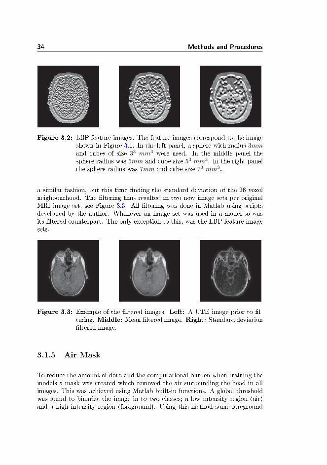
34 Methods and Procedures
Figure 3.2: LBP feature images. The feature images correspond to the imageshown in Figure 3.1. In the left panel, a sphere with radius 3mmand cubes of size 33 mm3 were used. In the middle panel thesphere radius was 5mm and cube size 53 mm3. In the right panelthe sphere radius was 7mm and cube size 73 mm3.
a similar fashion, but this time �nding the standard deviation of the 26 voxelneighbourhood. The �ltering thus resulted in two new image sets per originalMRI image set, see Figure 3.3. All �ltering was done in Matlab using scriptsdeveloped by the author. Whenever an image set was used in a model so wasits �ltered counterpart. The only exception to this, was the LBP feature imagesets.
Figure 3.3: Example of the �ltered images. Left: A UTE image prior to �l-tering. Middle: Mean �ltered image. Right: Standard deviation�ltered image.
3.1.5 Air Mask
To reduce the amount of data and the computational burden when training themodels a mask was created which removed the air surrounding the head in allimages. This was achieved using Matlab built-in functions. A global thresholdwas found to binarize the image in to two classes; a low intensity region (air)and a high intensity region (foreground). Using this method some foreground

3.2 Gaussian Mixture Regression 35
areas were classi�ed as air, so morphological operations were applied to removethese spots. Lastly, connected component analysis was used to determine whichregion was foreground and which was air. The air mask was derived from themean �ltered version of echo 1 of the high angle dUTE image and applied toall corresponding image sets. The result was visually inspected to ensure thatno important structures were removed. An example of the air mask is shown inFigure 3.4.
Figure 3.4: Example of the air mask. The green area is the air mask andeverything outside this area is excluded from the images.
3.1.6 De�ning the Input/Output Data for the Models
Once the pre-processing was done, the training data for the models was de�ned.Models with dUTE only, with dUTE+mDixon and with dUTE+LBP input wereto be trained. The dUTE only model consisted of 12 input variables, namelya dUTE acquisition at 10◦ (2 image sets), a dUTE acquisition at 25◦ (2 imagesets) and their �ltered images (8 image sets). The dUTE+mDixon model hadin addition to the aforementioned images, an mDixon water and an mDixon fatimage set and their �ltered versions as input thus yielding 18 input variablesin total. The model with dUTE+LBP consisted of the same input variables asthe dUTE only model but with the addition of 3 LBP image sets per originaldUTE image set. This resulted in a total of 24 input variables.
The output variable was in all cases the CT image set.
3.2 Gaussian Mixture Regression
AMatlab implementation of Gaussian mixture regression, [38], was used through-out this project. The implementation utilized the built-in k-means function ofthe Matlab Statistics toolbox to give an initial estimate of the component mean

36 Methods and Procedures
values and covariance matrices for the EM algorithm. Initial seeds for the k-means algorithm were chosen at random. EM was stopped when the increase inlog likelihood was smaller than 10−10.
3.2.1 mDixon Input Study
To evaluate the impact of using mDixon images as an additional input for theGMR model, dUTE only and dUTE+mDixon models were trained for compar-ison. A leave-one-out approach was taken. This meant that each model wastrained on data from two patients and then applied to the third to predict apCT. In this way three pCTs were predicted from dUTE+mDixon models andthree from dUTE only models. Following the method of Johansson et al., [5,16],20 components were used for estimating all GMMs.
3.3 Random Forest Regression
The Matlab built-in implementation called TreeBagger, was used for RaFR.With the parameter settings used in this project, TreeBagger is identical toBreiman's version of the Random Forest framework as described earlier. Forrandomization of the individual trees, a combination of bootstrap aggregating(bagging) and random node optimization was used. This meant that only afraction of the total training data was used to train each tree and that only onethird of the input variables were chosen at random at each node to determinethe best split.
3.3.1 Model Optimization Study
In this study the optimal tree depth for pCT generation was investigated. Inthe Matlab RaF implementation, the tree depth was controlled implicitly by theminimum leaf size parameter. This parameter controlled the minimum amountof data that should be in a node before it was declared a leaf. As such, the userhad no direct control over the tree depth. The Matlab implementation provideda method for estimating the optimal minimum leaf size. This consisted of storingwhich data was out-of-bag (i.e. the data not used to train each tree) for eachtree and then using this as test data to make an estimate of the predictionerror. Using this method, 5 regression forests each with 25 trees were trainedon one patient (h01) and the out-of-bag data was used to calculate the MSPD

3.4 Post-processing 37
as a function of the number of trees. The input variables were dUTE+mDixonimage sets. The minimum leaf size was set to 5, 10, 20, 50 or 100 in the forestsfor comparison.
3.3.2 LBP Input Study
In this study the e�ect of using the 3D LBP feature image sets as an input tothe RaFR model was investigated. Three RaFs were trained on data from onepatient (h01) using 25 trees in each forest and a leaf size of 10. One forest hadthe dUTE image sets as input, one had the dUTE image sets along with theircorresponding LBP feature image sets as input and one had the dUTE+mDixonimage sets as input. The models were tested on data from another patient (h03)to predict the pCTs.
3.3.3 mDixon Input Study
As in the mDixon input study of the GMR model the impact of using mDixonimages in the RaFRmodel was evaluated by training dUTE only and dUTE+mDixonmodels for comparison. Again a leave-one-out approach was used to estimatethree pCTs using mDixon images and three without them. A forest consistingof 80 trees with a minimum a leaf size of 10 was used.
3.4 Post-processing
3.4.1 Prediction Deviation
For the mDixon input studies and LBP input study, the MAPD and MPDin bins of 20 HU were calculated to quantify the prediction errors made inspeci�c intensity ranges of the real CT image set when using the additionalinput and when not using the additional input. Furthermore the MAPD forthe entire image sets and for the voxels inside the air mask was calculated inorder to be able to compare the overall accuracy of the di�erent models. Thesecomputations were all carried out in Matlab.
38 Methods and Procedures
3.4.2 Geometric Evaluation
The results from the mDixon input studies were evaluated geometrically usingthe Dice coe�cient and the Miss% and False%. These values were computedby importing the pCTs and real CTs into Varian Eclipse Treatment PlanningSystem software. Here, the bone voxels in the image sets were automaticallysegmented. The software provided tools for �nding the intersection between thebone regions of the pCT and the real CT, as well as for measuring the volume ofthese regions. These quantities were used to calculate the Dice coe�cient andMiss% and False% as described earlier.
3.4.3 Dose Plan and DVHs
For the mDixon input studies, a dosimetric evaluation of the pCTs of patienth03 was performed. The cerebrum, eyes and Hippocampus were automaticallysegmented on the T1 weighted image set. A Volumetric Modulated Arc Therapy(VMAT) dose plan was set up and optimized in Varian Eclipse Treatment Plan-ning System following the standard clinical procedure at Herlev. The cerebrumwas the planning target volume (PTV) and the eyes and Hippocampus wereplanning risk volumes (PRVs). 30 Gy was to be delivered in 10 fractions using 2arcs with an output of 286 and 285 Monitor Units (MU), respectively. The sim-ulated delivered dose was calculated using the CT (considered the true delivereddose) and pCTs and DVHs of the PTV and PRVs were made. D98%, Dmedian,D2% and Dmean DVH points were noted. The dose plan was pre-clinical, in thesense that no oncologist veri�ed the dose distributions or the appearance of theautomatically segmented structures.

Chapter 4
Results
The results are presented in 3 sections. One with the result of the RaF modeloptimization, one which focuses on the impact of using the LBP feature in RaFRand one which focuses on the impact of the mDixon input for both GMR andRaFR.
4.1 Random Forest Model Optimization
In Figure 4.1 the MSPD has been plotted as a function of the number of treesin a forest. 5 forests were trained with di�erent terminal leaf size. This studywas carried out to decide which leaf size should be used in the later studies. Nomarked di�erence was observed at 25 trees, when using a leaf size of 5 or 10,so 10 was chosen because shallower trees should be faster to train than deeperones. It is seen that as the number of trees increases, the MSPD decreases andconverges towards a constant value.

40 Results
0 5 10 15 20 250.1
0.2
0.3
0.4
0.5
0.6
0.7
0.8
0.9
1
Number of Trees
norm
aliz
ed M
SP
D
5102050100
Figure 4.1: The mean squared prediction deviation as function of the numberof trees in the forest for �ve forests with leaf sizes of 5, 10, 20, 50or 100.

4.2 Random Forest LBP Input 41
4.2 Random Forest LBP Input
In Figure 4.2 the MAPD and MPD have been plotted as a function of the realCT value (calculated in bins of 20 HU) for comparison of a model with dUTEonly input and one with dUTE+LBP input. It is observed, that in the airregion (-1000 HU), the MAPD is lowest for dUTE+mDixon and highest fordUTE+LBP. In the range −700-−100 HU the MAPD is lowest for dUTE+LBPand highest for dUTE+mDixon. In the range 500-1500 HU the MAPD is lowestfor dUTE+mDixon and highest for dUTE only. It is observed from the MPD,that the di�erences in MAPD are mainly due to systematic errors, i.e. a con-sistent overestimation of air and underestimation of bone ( in the 700+ HUrange). In table 4.1, the MAPDs are shown for the three pCTs. It is observedthat the error is lowest for dUTE+mDixon and highest for dUTE+LBP whenlooking at the entire image sets. When only looking in the region inside the airmask, the error is still lowest for dUTE+mDixon but highest for dUTE only. Itis observed that including the air region increases the MAPD for dUTE+LBPand decreases it for dUTE+mDixon and dUTE only.
-1000 -500 0 500 1000 15000
100
200
300
400
500
600
700
800
900
1000
Real CT Number [HU]
Mea
n ab
solu
te p
redi
ctio
n de
viat
ion
[HU
]
dUTE onlydUTE+LBPdUTE+mDixon
-1000 -500 0 500 1000 1500-1000
-800
-600
-400
-200
0
200
Real CT Number [HU]
Mea
n pr
edic
tion
devi
atio
n [H
U]
dUTE onlydUTE+LBPdUTE+mDixon
Figure 4.2: The MAPD (left) and MPD (right) as a function of the real CTvalue (calculated in bins of 20 HU) for models using dUTE only,dUTE+LBP and dUTE+mDixon input.
dUTE only dUTE+LBP dUTE+mDixonMAPD, entire image 121.7 HU 184.3 HU 81.1 HUMAPD, inside air mask 145.9 HU 133.0 HU 122.6 HU
Table 4.1: The mean absolute prediction deviation for the entire image setsand inside the air mask for models using dUTE only, dUTE+LBPand dUTE+mDixon input.

42 Results
4.3 mDixon Input Study
The results of the mDixon input variable studies for both models have beencollected in this section.
4.3.1 Prediction Deviations
In Figure 4.3 the MAPD and MPD have been plotted as a function of the realCT value (calculated in bins of 20 HU) for the three patients. In the top panels(4.3a) the results for GMR with and without mDixon are shown and in thebottom panels (4.3b) the same are shown for RaFR.
Looking at the top panels (GMR), similar patterns are observed both with andwithout the mDixon: the absolute error is observed to be low when predict-ing CT values around −1000 HU and 0 HU. Looking at the impact of usingdUTE+mDixon, for two patients the MAPD is observed to be lower in the 500-1000 HU range for the dUTE+mDixon pCTs compared to the dUTE only. Inthe 1000-1500 range the opposite is the case. The MPD, which as mentioned canquantify the systematic errors, reveals that the absolute error seen in the rangesfrom −1000 HU to −100 HU and 250-1500 HU is mainly due to a consistentunderestimation of the real CT value.
Looking at the bottom panels (RaFR), a lower MAPD is observed for thedUTE+mDixon compared to the UTE only in the 500-1500 HU range. Lookingat the MPD, it is observed that the systematic error is also lower (closer to 0)for the UTE+mDixon compared to the UTE only in the 500-1500 HU range.
In Table 4.2, the mean absolute prediction deviation is shown for all predictedpCTs using RaFR and GMR with dUTE+mDixon or dUTE only as inputs.Results calculated for the entire image sets (top half) and inside the region ofthe air mask (bottom half) are shown. When looking at the entire image set,on average GMR with dUTE only has the lowest overall absolute error followedby RaFR with dUTE+mDixon. It is seen that RaFR with dUTE+mDixon hasthe lowest standard deviation. Looking at the the region inside the air mask,on average, RaFR with dUTE+mDixon has the lowest error, followed by GMRwith dUTE+mDixon, RaFR with dUTE only and GMR with dUTE only.

4.3 mDixon Input Study 43
-1000 -500 0 500 1000 15000
100
200
300
400
500
600
700
800
900
1000
Real CT Number [HU]
Mea
n ab
solu
te p
redi
ctio
n de
viat
ion
[HU
]
dUTE+mDixondUTE Only
-1000 -500 0 500 1000 1500-1000
-800
-600
-400
-200
0
200
Real CT Number [HU]
Mea
n pr
edic
tion
devi
atio
n [H
U]
dUTE+mDixondUTE Only
(a) GMR
-1000 -500 0 500 1000 15000
100
200
300
400
500
600
700
800
900
1000
Real CT Number [HU]
Mea
n ab
solu
te p
redi
ctio
n de
viat
ion
[HU
]
dUTE+mDixondUTE Only
-1000 -500 0 500 1000 1500-1000
-800
-600
-400
-200
0
200
Real CT Number [HU]
Mea
n pr
edic
tion
devi
atio
n [H
U]
dUTE+mDixondUTE Only
(b) RaFR
Figure 4.3: The MAPD (left) and MPD (right) as a function of the real CTvalue (calculated in bins of 20 HU) for the pCTs for the threepatients. The top panels are for GMR and the bottom panels arefor RaFR.

44 Results
Entire image setGMRdUTE+mDixon
GMRdUTE only
RaFRdUTE+mDixon
RaFRdUTE only
MAPD, h01 68.7 HU 67.9 HU 70.0 HU 69.5 HUMAPD, h02 75.0 HU 73.4 HU 70.0 HU 88.2 HUMAPD, h03 70.3 HU 65.6 HU 69.3 HU 78.7 HUMean value 71.3(±2.65)HU 69.0(±3.25)HU 69.8(±0.32)HU 78.8(±7.62)HU
Inside air maskGMRdUTE+mDixon
GMRdUTE only
RaFRdUTE+mDixon
RaFRdUTE only
MAPD, h01 127.3 HU 133.4 HU 112.2 HU 125.6 HUMAPD, h02 128.1 HU 142.1 HU 112.8 HU 137.6 HUMAPD, h03 128.1 HU 139.3 HU 113.2 HU 134.5 HUMean value 127.8(±0.4)HU 138.3(±3.6)HU 112.7(±0.4)HU 132.6(±5.1)HU
Table 4.2: The mean absolute prediction deviation (MAPD) calculated foreach predicted pCT using the di�erent regression models. Also themean MAPD for each method with one standard deviation con�-dence interval is shown. Values calculated for the entire image setsand for voxels inside the air mask are shown.
4.3.2 Geometric Evaluation
In Table 4.3 theMiss%, False% and Dice score for the individual patients alongwith the average when using GMR and RaFR is shown. It is observed that thegeneral tendency for the individual patients is a lowerMiss% and False% and ahigher Dice score when using dUTE+mDixon compared to dUTE only. This isthe case for both GMR and RaFR and is further con�rmed by the mean valuescomputed over all three patients. It is also observed that on average, the pCTspredicted using RaFR with dUTE+mDixon input have the lowest Miss% andFalse% and highest Dice score. This is also the method that shows the loweststandard deviation. On average GMR using dUTE only produces the highestMiss% and False% and lowest Dice score.

4.3 mDixon Input Study 45
GMRdUTE + mDixon dUTE only
h01, Miss% 18.3% 26.0%h02, Miss% 16.7% 17.4%h03, Miss% 23.4% 27.3%h01, False% 31.5% 31.1%h02, False% 26.2% 33.4%h03, False% 29.0% 30.8%h01, Dice 0.75 0.71h02, Dice 0.78 0.74h03, Dice 0.74 0.71Mean Miss% 19.5%(±3.48%) 23.6%(±5.44%)Mean False% 28.9%(±2.63%) 31.7%(±1.42%)Mean Dice 0.76(±0.38) 0.72(±0.02)
RaFRdUTE + mDixon dUTE only
h01, Miss% 20.3% 25.8%h02, Miss% 13.9% 16.1%h03, Miss% 17.5% 24.9%h01, False% 22.1% 26.8%h02, False% 22.4% 30.2%h03, False% 22.3% 28.7%h01, Dice 0.79 0.74h02, Dice 0.82 0.76h03, Dice 0.80 0.74Mean Miss% 17.2%(±3.22%) 22.0%(±5.14%)Mean False% 22.3%(±0.15%) 28.6%(±1.75%)Mean Dice 0.80(±0.01) 0.75(±0.01)
Table 4.3: Bone miss percentage, false bone percentage and Dice score forGMR and RaFR with and without mDixon input for the threepatients. The values below the dashed lines are the mean valuescalculated over all three patients with one standard deviation con-�dence limits in parentheses.
46 Results
4.3.3 Dosimetric Evaluation
The dosimetric evaluation was performed for patient h03. In Figure 4.4, thedose-volume histograms of the planning target volume (PTV) and planning riskvolumes (PRVs) (eyes and Hippocampus) for CT and pCT based dose calcu-lations are shown. From a visual inspection, it is observed that the largestdi�erences are present in the eye volume for both RaFR and GMR. It is hardto see if there are any di�erences between using dUTE+mDixon or dUTE only.
In Table 4.4, the DVH points, D98%, Dmedian, D2% and Dmean, are shownfor the three volumes of Figure 4.4 along with the percent deviation betweenthe points estimated from the pCT based doses and the CT based doses. It isobserved that all deviations are smaller than 2 %. When a deviation is observedin the PTV it is due to an underestimation of the true dose at D98% and dueto an overestimation at Dmedian and D2%. For the eyes and Hippocampus, thedeviation in Dmean is due to an underestimation of the true dose and in D2% itis due to an overestimation.

4.3 mDixon Input Study 47
0 5 10 15 20 25 300
10
20
30
40
50
60
70
80
90
100
Rat
io o
f tot
al s
truc
ture
vol
ume
[%]
Absolute Dose [Gy]
PTVEyesHippocampusCT dosedUTE+mDixon dosedUTE only dose
(a) Comparison of GMR models.
0 5 10 15 20 25 300
10
20
30
40
50
60
70
80
90
100
Rat
io o
f tot
al s
truc
ture
vol
ume
[%]
Absolute Dose [Gy]
PTVEyesHippocampusCT dosedUTE+mDixon dosedUTE only dose
(b) Comparison of RaFR models.
Figure 4.4: Dose-volume histograms. The cerebrum was the planning targetvolume (blue) and the eyes (red) and hippocampus (green) werethe planning risk volumes. The CT calculated dose is markedwith triangles for comparison with the dose calculated based onpCTs from models using dUTE+mDixon (squares) and dUTE only(circles).
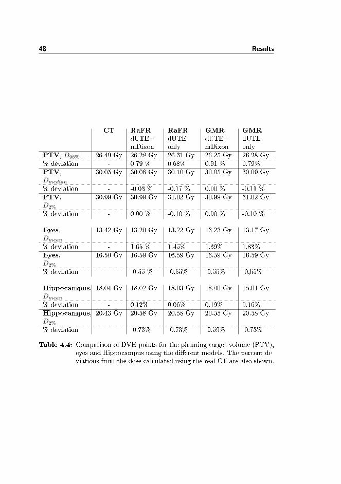
48 Results
CT RaFRdUTE+mDixon
RaFRdUTEonly
GMRdUTE+mDixon
GMRdUTEonly
PTV, D98% 26.49 Gy 26.28 Gy 26.31 Gy 26.25 Gy 26.28 Gy% deviation - 0.79 % 0.68% 0.91 % 0.79%PTV,Dmedian
30.05 Gy 30.06 Gy 30.10 Gy 30.05 Gy 30.09 Gy
% deviation - -0.03 % -0.17 % 0.00 % -0.11 %PTV,D2%
30.99 Gy 30.99 Gy 31.02 Gy 30.99 Gy 31.02 Gy
% deviation - 0.00 % -0.10 % 0.00 % -0.10 %
Eyes,Dmean
13.42 Gy 13.20 Gy 13.22 Gy 13.23 Gy 13.17 Gy
% deviation - 1.65 % 1.45% 1.39% 1.83%Eyes,D2%
16.50 Gy 16.59 Gy 16.59 Gy 16.59 Gy 16.59 Gy
% deviation - -0.55 % -0.55% -0.55% -0,55%
Hippocampus,Dmean
18.04 Gy 18.02 Gy 18.03 Gy 18.00 Gy 18.01 Gy
% deviation - 0.12% 0.06% 0.19% 0.16%Hippocampus,D2%
20.43 Gy 20.58 Gy 20.58 Gy 20.55 Gy 20.58 Gy
% deviation - -0.73% -0.73% -0.59% -0.73%
Table 4.4: Comparison of DVH points for the planning target volume (PTV),eyes and Hippocampus using the di�erent models. The percent de-viations from the dose calculated using the real CT are also shown.

4.3 mDixon Input Study 49
4.3.4 Comparing GMR and RaF
In Figure 4.5a the MAPD and MPD have been plotted as a function of thereal CT value (calculated in bins of 20 HU) for RaFR and GMR both usingdUTE+mDixon input. It is observed that the MAPD is lower for RaFR forhigh density CT values (1000-1500 HU). Also the MPD is closer to 0 in thatrange for RaFR. It is seen that in the range from approximately -700 HU to-400 HU the MPD is closer to zero for GMR. In Figure 4.5b the same is shownas in Figure 4.5a, but for models with dUTE only. Here, it is observed that theMAPD is lower for two of the patients for CT values of 1000+ HU using GMR.
In Figure 4.6, the pCTs and real CT from patient h03 are shown for three axialslices through the head. It is observed that noise is present in the air region ofthe pCTs predicted using dUTE+mDixon. A few di�erences between the pCTsand the real CT should be noted. First of all, the �xation device seen in thereal CT is not present in the pCTs. Secondly, the streak artefact due to dental�llings seen in the real CT is not present in the pCTs (although the tooth fromwhich it originates has a di�erent intensity than the rest of the teeth). In themiddle row of Figure 4.6, it is seen that to various degrees, the pCTs su�er fromerrors in the nasal region, the paranasal sinuses and in the ear region.

50 Results
-1000 -500 0 500 1000 15000
100
200
300
400
500
600
700
800
900
1000
Real CT Number [HU]
Mea
n ab
solu
te p
redi
ctio
n de
viat
ion
[HU
]
GMRRaFR
-1000 -500 0 500 1000 1500-1000
-800
-600
-400
-200
0
200
Real CT Number [HU]
Mea
n pr
edic
tion
devi
atio
n [H
U]
GMRRaFR
(a) With mDixon input.
-1000 -500 0 500 1000 15000
100
200
300
400
500
600
700
800
900
1000
Real CT Number [HU]
Mea
n ab
solu
te p
redi
ctio
n de
viat
ion
[HU
]
GMRRaFR
-1000 -500 0 500 1000 1500-1000
-800
-600
-400
-200
0
200
Real CT Number [HU]
Mea
n pr
edic
tion
devi
atio
n [H
U]
GMRRaFR
(b) Without mDixon input.
Figure 4.5: Comparison of RaFR and GMR, with and without mDixon input.The MAPD (left) and MPD (right) plotted as a function of thereal CT value (calculated in bins of 20 HU).

4.3 mDixon Input Study 51
(a)RealCT
(b)pCT,RaFR
dUTE+mDixon
(c)pCT,RaFR
dUTEonly
(d)pCT,GMR
dUTE+mDixon
-100
0
-500
0500
1000
1500
-100
0
-500
0500
1000
1500
HU
-100
0
-500
0500
1000
1500
(e)pCT,GMR
dUTEonly
Figure
4.6:ColumnwisevisualcomparisonofthepCTsandtherealCTfrompatienth03.Thetoprowshow
saninferior
(low
er)axialsliceofthehead.Themiddlerowshow
samedialaxialslice.
Thebottomrowshow
sasuperior
(upper)axialslice.

52 Results

Chapter 5
Discussion
5.1 Random Forest Model Optimization Study
The purpose of this study was to �nd a suitable tree depth for pCT predictionusing RaFR. As mentioned, this involved looking at the minimum leaf size. Themean squared prediction deviation (MSPD) as a function of the number of treeswas shown in Figure 4.1 for forests with a minimum leaf size of 5, 10, 20, 50 or100 data points. It was observed that using 5 or 10 data points produced thelowest MSPD using 25 trees, so 10 was chosen as the optimal minimum leaf sizedue to the theoretically faster training and testing using shallow trees comparedto deep ones. Figure 4.1 also serves to demonstrate one of the properties of theRaF framework: as the number of trees increases the prediction error decreasestowards a constant value. The out-of-bag data for each tree was sampled withreplacement so as the number of trees increased, the number of weak predictionsmade with the same input data also increased. Therefore, what is shown is thatas the number of weak predictions increases the �nal prediction error decreases.The optimization study was meant as a preliminary study to �nd an estimateof the optimal tree depth before training the �nal models. The training wasperformed on data from one patient and with 25 trees in each forest. Thismay pose a problem to the generalisability of the results, i.e. the data fromone patient may not be representative of the entire population of data and thetrend in the MSPD curves may change for forests of more than 25 trees. This, of

54 Discussion
course, should be considered before drawing any �nal conclusions on the optimalminimum leaf size. A more thorough study, using data from more patients anda forest size closer to the one used for actual pCT prediction could be carriedout in the future.
5.2 Random Forest Local Binary Pattern Input
Study
This study was carried out in order to investigate if the LBP feature imagesets could improve the prediction accuracy of RaFR. It was observed in Figure4.2 that in the air region (-1000 HU), the model with LBP feature image setshad a larger MAPD and MPD compared to models with dUTE+mDixon anddUTE only input. This can probably be explained by the air mask used to limitthe training data amount prior to training the models. Because the LBP of avoxel contains information about the neighbourhood of that voxel, air voxelsclose to the head have a di�erent LBP value than those far from the head thatare surrounded only by other air voxels. When the air mask was applied tothe training data, it essentially removed all the air voxels that were spatiallyfar from the head. Because the training data lacked these voxels, the resultingmodel was not trained to handle their LBP value, resulting in prediction errorsin those voxels. The error is clearly seen in Figure 5.1, where a dark �halo� ofcorrectly predicted air values surround the head but further away, the air voxelsare overestimated. A solution to this problem could be to assign a bulk intensityvalue of -1000 HU to all pCT voxels outside the air mask.In Figure 4.2, it was seen that in the range from approximately−700 HU to−100HU, the model with dUTE+LBP input had the lowest MAPD. In theory, lungtissue is the only tissue type in this Houns�eld range, so voxels of this intensityshould not be present in the head region of the body. From inspection of the realCTs used in this project, it was found that voxels of these intensities were placedin transition regions going from air to tissue. Instead of a sharp transition, asmooth gradient was observed, which lead to intensity values between -1000HU and -100 HU. These regions of smooth transitions were observed along allsuch edges, meaning on the entire periphery of the head and in the air cavitiesinside the head. It was investigated whether the smoothing artefact was dueto the interpolation done when registering and reslicing the CT image sets tothe dUTE image sets. This was not the case, since it was also present in theunprocessed CT images. It was thus assumed that the artefact was introducedin the CT acquisition phase. From the error curves in Figure 4.2, it seems thatthe model with the LBP feature is better able to mimic this property of the realCT compared to the models without it.

5.2 Random Forest Local Binary Pattern Input Study 55
HU-1000
-500
0
500
1000
1500
Figure 5.1: Example of air mask related prediction error when using LBP fea-ture image sets. The shown pCT was predicted using dUTE+LBPinput. As can be seen, the value of the air voxels far from the headis overestimated.
The three models showed similar error-wise behaviour in the soft tissue region(-100 HU to 500 HU), with the exception that the model with dUTE only inputhad larger errors in the 500 HU area.
When looking at the error in the bone range (500+ HU), the model withdUTE+LBP input had a performance between that of the models with dUTEonly input (worst) and dUTE+mDixon input (best). It was closest to thedUTE+mDixon curve in the range from 500 HU to 1000 HU and the dUTEonly curve from 1000 HU to 1500 HU. From this, it seems that adding the LBPfeature input improves the prediction accuracy in the bone region compared tousing dUTE only.
Due to the prediction errors made outside the air mask when using the dUTE+LBPinput, the MAPDs shown in Table 4.1 were calculated both for the entire pCTand for the voxels inside the air mask. When looking at the entire image sets, therelatively large error observed for the model with dUTE+LBP input is mainlycaused by all the air voxels far from the head which were overestimated. Whenlooking at the head region only (inside the air mask), it was seen that the modelwith dUTE+LBP input performs better than the one with dUTE only inputand worse than the model with dUTE+mDixon input. This con�rms what wasobserved in the error curves of Figure 4.2.
Summary: It seems to be possible to get better predictions when using theLBP feature image sets as an additional input compared to using dUTE only

56 Discussion
input. This may be attributed to the neighbourhood information that theseimage sets contain. Still, using the dUTE+mDixon input resulted in betteroverall predictions than using the dUTE+LBP input. An advantage of the LBPfeature image sets is that they are derived directly from the dUTE images, so noadditional scans are needed. A reduction in scan time is thus obtained comparedto using the mDixon input. Given this fact and the results shown, the methodlooks promising although further studies using more data and a larger forestshould be carried out.
5.3 mDixon Input Study
The RaFR LBP input study already suggested that using the mDixon inputproduced better predictions compared to using dUTE only input. In this studya more thorough investigation of the mDixon input was carried out using moredata and a larger forest. Furthermore, the use of GMR for pCT prediction usingboth dUTE+mDixon and dUTE only input was investigated. All resulting pCTswere evaluated thoroughly using both the prediction deviation, Dice score anddosimetric deviation.
5.3.1 Gaussian Mixture Regression
The piecewise deviations of the pCTs from the real CT value was shown inFigure 4.3a for GMR using dUTE+mDixon and dUTE only input. From theMAPD and MPD error curves it was hard to determine whether the GMRmodel was improved when using the mDixon input. In one region (500-1000HU) the predictions were better (for two patients) but in another they wereworse (1000-1500 HU).
When looking at the MAPDs in Table 4.2, the di�erence between using mDixonor not for the entire image sets seems relatively small. When looking in thecon�ned region of the air mask, however, the di�erence is larger and consistentlyin favour of using the mDixon input. From visual inspection of the pCTs, itwas noticed that when using the mDixon input, predictions in the surroundingair region was more a�ected by errors than when using dUTE only input (seeFigure 4.6). It was also observed that the mDixon image sets themselves were,in general, more in�uenced by noise in air voxels than the dUTE image sets (thenoise in the air voxels can be seen in Figure 2.2). This may be attributed tothe post-processing done to these image sets in order to derive the water-onlyand fat-only image sets. The noise may be the reason that the models with

5.3 mDixon Input Study 57
mDixon input do not show smaller errors than models with dUTE only inputwhen looking at the entire image sets. Again, one could consider assigning abulk value of -1000 HU to all pCT voxels outside the air mask.
As mentioned in the introduction, the GMR model has previously been usedby Johansson et al. to predict pCTs [5, 16]. One of the goals of this projectwas to investigate the robustness of the model and the ability to reproduce theresults in a di�erent clinical set-up (e.g. using a 1 T MRI scanner instead of a1.5 T MRI scanner). Johansson et al. reported an average MAPD inside the airmask of 137 HU with a minimum of 117 HU and maximum of 176 HU for theindividual patients. Their study included 5 patients and used dUTE input aswell as an additional T2 weighted MRI image set (which was later found to beredundant). In the present study, the average MAPD inside the air mask wasfound to be 138.3 HU for dUTE only input, which is close to what Johansson et
al. reported. Johansson et al. also did a piecewise evaluation of the error usingthe MAPD and MPD calculated in bins of 20 HU. However, they calculatedthe error curves as a function of the predicted CT value and not the real CTvalue (as done in this report) so a direct comparison was not possible. Still, theoverall MAPD results were comparable and also from a visual inspection theresults obtained in this project look similar to those reported by Johansson et
al. The di�erence in clinical set-up thus seems to not a�ect the accuracy of thepredicted pCTs as long as the GMR model is trained on data from the speci�cclinical set-up that it should be used in.
The geometrical evaluation showed a tendency in favour of using the mDixoninput. Referring to Table 4.3, the boneMiss% for each patient pCT was consis-tently lower for models using the mDixon input compared to models with dUTEonly input. Except for the pCT of patient h01, the same was the case for thebone False%. Furthermore, the Dice coe�cient was higher for all pCTs whenusing mDixon input, suggesting a better geometrical accuracy of bone in theseimage sets. This in turn should lead to DRRs more similar to those generatedwith the real CT.
Looking at the DVHs in Figure 4.4a, it was clear that the largest dosimetricdeviation was present in the eyes. It was not possible to visually distinguish theDVHs originating from the model with dUTE+mDixon input and the modelwith dUTE only input. Looking at the DVH points in Table 4.4, the visuallylarge deviations observed for the eye volume was con�rmed by > 1% deviationsin Dmean for that volume for both models with and without mDixon input.Inspection of the pCTs of patient h03 revealed that parts of both eyes weregiven a bone density value, so this may be the reason for the deviations. Ingeneral, all deviations were < 2% and the di�erence between using mDixoninput and dUTE only input was not obvious.

58 Discussion
Summary: The reproducibility of results when using a GMR model with dUTEinput was demonstrated in this study. From the results obtained, there wasan indication that the addition of the mDixon input could improve both theprediction accuracy and the geometric accuracy. The dosimetric accuracy waswithin 2 % for models both with and without mDixon input.
5.3.2 Random Forest Regression
Looking at the MAPD and MPD curves in Figure 4.3b, it was seen that usingthe mDixon input improved the prediction accuracy for CT values above 500HU. In Table 4.2, the MAPDs for both the entire image sets and for voxelsinside the air mask were lower when using the mDixon input. The di�erencewas more distinct when looking inside the air mask. As was the case for GMR,the pCTs predicted with RaFR using mDixon input had more noise in the airregion which may be what caused this behaviour.
The geometric evaluation showed the same tendency as the prediction devia-tions. Using the mDixon input resulted in consistently lower bone miss volumesand false bone volumes and a higher Dice score compared to not using it.
As with GMR, the DVHs showed the largest deviations in the eye volume, whichwas con�rmed by the Dmean DVH points in Table 4.4. Again, the pCTs revealedthat some voxels in the eyes were given a bone density value, which may be thereason for the deviations. It was hard to spot a clear tendency from the DVHpoints in favour of using mDixon input. The deviations were < 1.7% for allDVH points.
Summary: The impact of using mDixon image sets as an additional inputto a RaFR model was demonstrated. It was found that using mDixon inputimproved the prediction accuracy and geometric accuracy of the models. It wasnot possible to conclude whether the dosimetric accuracy was improved whenadding mDixon input.
5.3.3 Comparing GMR and RaFR
In Figure 4.5a, the MAPD and MPD curves were shown for GMR and RaFRmodels with mDixon input. For high density values, the RaFR model had thelowest MAPD. In Figure 4.5b, the same curves were shown for models withdUTE only input with an indication that the GMR model performed better inthe high density region.

5.3 mDixon Input Study 59
Looking at the MAPD inside the air mask in Table 4.2, RaFR using mDixoninput consistently produced the lowest error. On average, the next best modelwas GMR with mDixon input followed by RaFR with dUTE only input andlastly GMR with dUTE only input.
From a geometrical viewpoint, RaFR with dUTE+mDixon input produced thebest results. The worst results were obtained with GMR using dUTE onlyinput. Which one of GMR with dUTE+mDixon input and RaFR with dUTEonly input performed the best was not clear.
Looking at the DVHs and DVH points, it was hard to decide which modelto prefer. The largest deviation from the CT based dose was 1.83 % and thedi�erence in the individual deviations was a maximum of 0.38 percentage points.It should be investigated whether these numbers are signi�cant. For the eyevolume all pCTs showed the largest dosimetric deviation from the real CT. Asalready touched upon, prediction errors were present in the eyes causing somevoxels to appear as bone. This is probably what caused the dose distributionto appear less homogeneous in this volume.
When looking at prediction deviations in the air mask and the geometricalaccuracy, the results were mostly in favour of using RaFR with mDixon inputcompared to any GMR model and RaFR with dUTE only input. This meansthat the pCTs produced with this model would probably produce the mostsatisfactory DRRs. The next best models were GMR with dUTE+mDixon inputand RaFR with dUTE only input. Because the dosimetric evaluation was lessconclusive, the question arises whether the improvement in geometrical accuracyis worth the extra scan time that the mDixon sequence requires (approximately2.5 minutes). It could be that the geometrical accuracy of one of the dUTE onlymodels is su�cient for creating usable DRRs. The RaFR model with dUTE onlyinput had an almost similar Dice score to the GMR model with dUTE+mDixonso it may be worth investigating if this model produces su�cient pCTs for RTplanning.
Another thing to take into account is the time e�ciency of the two regressionimplementations. On a Linux node with 2×2.66 GHz quad-core processors and24 GB memory, the current implementations of GMR and RaFR used on average50 hours to train a model using dUTE+mDixon data from two patients. Whenusing dUTE only data the time was reduced to approximately 35 hours. Topredict a new pCT took approximately 20 minutes for GMR and 5 hours forRaFR. These numbers speak in favour of using GMR.
It should also be noted that it was not investigated whether 20 components usedin the GMM was the optimal number suited for the task. The 20 componentswere chosen based on what Johansson et al. used in their study. It may be

60 Discussion
the case that when adding the mDixon input, more components are needed tomodel the joint distribution of MRI and CT intensities. A di�erent number ofcomponents could potentially improve the prediction performance of GMR.
5.3.4 General Comments on the pCTs
In Figure 4.6, axial slices of all the predicted pCTs and the real CT for patienth03 were shown. As already mentioned, the pCTs predicted with models usingmDixon input showed errors in the air region surrounding the head. This is mostclearly observed in the inferior axial slices shown in the top row of Figure 4.6.Another interesting thing to note in this row is that the streak artefact presentin the real CT is not predicted in the pCTs. This could be seen as an advantagebecause it would mean that such artefacts would not be present in the DRRsgenerated from pCTs. It should be noted that streak artefacts were present inall the CTs used in this project. Except for patient h02, these were not removedfrom the training data. Optimally, the models should be trained on imageswithout such artefacts, because they would then be better representations ofthe general appearance of a CT image. The pCTs were compared to the realCT when calculating the piecewise deviations. This included the region wherestreak artefacts were present and this could be the reason that for high densityvalues in the real CT the pCT has a large MAPD and MPD.
From inspection of the pCTs, it was observed that the regions with the largestvisual deviations from the real CT were found near the nose, ears and para-nasal sinuses. These are all regions with air-tissue interfaces so a reasonableexplanation could be that susceptibility artefacts in the MRI image sets arecausing this.
Using dUTE+mDixon input produced the lowest overall error inside the airmask for both GMR and RaFR, so it seemed that the mDixon image sets in-cluded some information that was not captured by the dUTE image sets. Aspreviously mentioned, the reason for using the mDixon water and fat imagesets, was to compensate for water/fat phase cancellation artefacts in the dUTEimage sets recorded on a 1 T scanner. These artefacts could cause non-bonevoxels to appear as bone. In other words the mDixon input should improve theprediction accuracy of non-bone voxels. The largest di�erence in the MAPDand MPD curves was observed in the bone region of the real CT which was notas expected. No reasonable explanation to this behaviour was found during thisproject.

5.4 Evaluation Methods 61
5.4 Evaluation Methods
In this section some of the limitations of the evaluation methods will be outlined.For all methods used in this report, one limitation is that the spatial informationis lost. This means that the methods cannot reveal in what spatial region ofthe image set an error is present. This information would be useful since itmay show in what regions the input MRI image sets lack information or arein�uenced by artefacts. From visual inspection of the pCTs, it seems that errorsare made in the paranasal sinuses, nose and ear regions. None of the evaluationmethods can back this up. The idea of calculating the MAPD for local regionswas carried out to some extend by using the air mask as a region, but it maybe useful to look into calculating errors in smaller regions in order to quantifythe local errors better. This could also be done for the geometric evaluation.A subtraction of the reference CT and pCT could also serve to show in whichspatial regions the errors are most profound.
5.4.1 Prediction Deviation Method
The MAPD and MPD computed in bins of 20 HU provide a tool for quanti-fying the errors made in speci�c voxel intensity ranges of the real CT. Takingadvantage of the Houns�eld scale, it is thus possible to quantify the errors madein speci�c tissues. To calculate the error at -500 HU, all voxels in the real CTwith an intensity of -510 HU to -490 HU along with the spatially correspondingvoxels in the pCT are used. This fact must be kept in mind when inspecting theMAPD and MPD curves, because, depending on the the number of voxels in abin, the error may be calculated based on 1 voxel or thousands of voxels. If it iscalculated based on a proportionally small number of voxels, a seemingly largeerror in a speci�c range may not a�ect the overall image much. This propertyof the error curves does not mean that they cannot be used to compare andelucidate the models' performance in the di�erent tissue regions, it means thatthey may not provide a measure of the overall prediction accuracy. To quantifythe overall prediction accuracy of the models, the MAPDs based on the entireimage set and on the region within the air mask have been calculated.
5.4.2 Geometric Evaluation Method
Even though all images were co-registered prior to training the models, the reg-istration was lost when the pCTs were imported into Varian Eclipse TreatmentPlanning System for geometric evaluation. For this reason a new registration

62 Discussion
had to be made. The geometrical agreement, as measured by the Dice coe�-cient, may include registration errors since it is a measure of the overlap betweenregions, which is a�ected by the registration. However, the same registrationwas applied to all pCTs belonging to a given patient, so if a registration errorwas present, the same error would be incorporated into all Dice scores of thesame patient. This means that the intra-patient Dice scores should be compa-rable, but one should keep in mind that when comparing inter-patient scoresthe di�erence may be attributed to di�erent quality of the registration.
5.4.3 Dosimetric Evaluation Method
The main limitation when using dose-volume histograms (DVHs) and DVHpoints for dosimetric evaluation is that even though each DVH is con�ned tospeci�c regions (PTV or PRVs), the spatial information within these regions islost. This means that if the simulated dose distributions in each volume aresimilar using CT and pCT, spatially local deviations in the estimated delivereddose may still exist. Comparing isodose contours in the CT and pCT couldprovide a spatial evaluation of the dosimetric deviations.
5.5 Future Work
One thing that can a�ect the quality of the pCT is the amount of data usedto train the regression models. The assumption when estimating the modelparameters from training data is that the data is representative of all futureinputs and outputs. If this is not the case, i.e. the training data representsa rarely observed case of all possible inputs and outputs, the resulting modelwill not be able to make good predictions on future inputs. Artefacts in theMRI and CT image sets, such as those originating from dental �llings, areexamples of patient speci�c deviations from the general appearance of inputand output data. Using data from many patients to train the models increasesthe probability that the majority of the training data is representative of futureinputs and outputs and should in turn lead to better predictions.In this report, the LBP input study was carried out by using data from onepatient and then predicting the pCT of another. The results presented in themDixon input studies were based on data from three patients using a leave-one-out approach. Adding more patient data to all these studies could improve theoverall predictions and may help to determine whether the observed trends areconsistent.

5.5 Future Work 63
When doing regression using GMR, it is possible to get an estimate of theconditional variance of the predictions. This is also possible for RaFR, if usingthe method of Criminisi et al. The variance could be used to show in whichregions of the pCT the predictions have a large uncertainty and in which they donot. Along the same line, Johansson et al. suggested that the expected absolutedeviation could be incorporated into the absorbed dose calculated using thepCT [16]. This would then give an estimate of the uncertainty of the calculateddose, which could be useful as a quality assurance measure. In this project, theconditional variance of the predictions was not investigated, so this is somethingto look into in the future.
A number of improvements could be made to the LBP implementation used inthis project. The LBP approach was inspired by the work by Pauly et al. whoused a 3-scale 3D LBP-like feature derived from Dixon MRI image sets to pre-dict organ bounding boxes [17]. In their description of the feature extraction,no details as to the radius of the spheres de�ning the neighbourhood or thesize of the 3D cubes was found. These two parameters are of vital importanceto the appearance of the resulting feature images, since they de�ne the scaleof the neighbourhood that is captured. In this project, it was not investigatedwhether the three scales used for feature extraction were the optimal for cap-turing textural information in the MRI image sets. Furthermore, because theLBP contains neighbourhood information, the rotation of the image sets a�ectsthe result. The current implementation is not rotation invariant, so this couldbe included to improve the robustness.
From an time-e�ciency point of view, especially the RaFR implementation hasroom for improvements. The built in Matlab implementation was run in serial,meaning that one tree was trained at a time. The RaF framework is an obviouscandidate for parallel computing because each tree is independent from theothers. This could improve the speed of both training and predicting. It wasnot possible to get the built in Matlab implementation to run in parallel, butour own implementation, used to generate the examples in Section 2.5, wassuccessfully run in parallel with marked improvements in speed as a result.
Finally, a clinical validation of the pCTs could be carried out in the future.This would include investigating if the geometrical accuracy is good enoughto generate satisfactory DRRs for patient alignment and investigating if thedosimetric deviations are signi�cant compared to a CT based plan.

64 Discussion

Chapter 6
Conclusion
In this project, Gaussian mixture regression (GMR) and Random Forest re-gression (RaFR) were investigated as a tool for obtaining pseudo-CTs (pCTs)from MRI image sets to use in MRI-only radiation therapy planning. dUTEand mDixon MRI image sets were investigated as input to both models andfor RaFR a Local Binary Pattern (LBP) feature input was investigated. Theresults were evaluated in terms of the voxel-wise deviations described by themean absolute prediction deviation (MAPD) and mean prediction deviation(MPD). A geometrical evaluation of bone in the pCTs was carried out using theDice coe�cient and the missed bone and false bone percentages. Furthermore,a dosimetric evaluation was carried out by comparing dose-volume histograms(DVHs) and DVH points based on pCT and CT dose calculations.
Gaussian Mixture Regression
GMR is a promising approach to generating pCTs. In this project the repro-ducibility of previously reported results was demonstrated in terms of a similaraverage MAPD. A new approach of adding mDixon image sets to the inputof the model showed to improve the prediction accuracy and geometrical ac-curacy of the predicted pCTs compared to using only dUTE image input. Anaverage Dice score of 0.76 for dUTE+mDixon models and 0.72 for dUTE only

66 Conclusion
models was obtained. In terms of the dosimetric accuracy, it was found thatthe absorbed dose calculations based on GMR pCTs had deviations of < 2% inclinically relevant DVH points compared to dose calculations based on CT. Noclear dosimetric di�erence was observed between adding the mDixon input andnot adding it.
Random Forest Regression
RaFR is another promising method which has not been used to generate pCTsprior to this project. For the implementation of RaFR used in this project, itwas found that using a minimum leaf size of 10 as stopping criteria for treegrowing resulted in the smallest mean squared prediction deviation (MSPD).It was investigated whether adding an LBP feature image as input could im-prove the pCTs. It was found that a dUTE+LBP input improved the predictionaccuracy compared to using only dUTE input. The results were based on a rela-tively small amount of data so further studies should be carried out. The impactof adding mDixon input was also investigated for RaFR. Here it was found thatusing dUTE+mDixon input improved the prediction accuracy and geometricalaccuracy of the pCT compared to using only dUTE input. An average Dicescore of 0.80 for dUTE+mDixon models and 0.75 for dUTE only models wasobtained. The dosimetric deviations between absorbed dose calculations basedon RaFR pCTs and real CT were found to be < 1.7% in clinically relevant DVHpoints.
Comparison of Gaussian Mixture Regression and RandomForest Regression
The RaFRmodel with dUTE+mDixon input produced the best pCTs in terms ofprediction accuracy and geometrical accuracy. The next best models were GMRwith dUTE+mDixon input and RaFR with dUTE only input. The extra scantime required with the mDixon input and the time e�ciency of the GMR andRaFR implementations should also be considered, before drawing conclusionsas to which model is preferred.
Future Work
The results presented in this report showed the potential of using GMR andRaFR for predicting pCTs. A number of things could be investigated in the

67
future. First of all, studies using more data could be done in order to verifythe trends observed in this report. An investigation of the signi�cance of thegeometric and dosimetric deviations could be carried out. This would also helpin determining if the improvement in geometrical accuracy observed with themDixon input is worth the extra scan time.
The LBP input study showed promising results but further investigation isneeded. Using feature images with neighbourhood information could prove tomake additional non-conventional MRI sequences like the mDixon redundant.

68 Conclusion

Appendix A
Abstract Accepted forESTRO Forum 2013

The impact of a Dixon sequence in creating a pseudo CT scan from MR
images using a Gaussian mixture regression model D. Andreasen1, J.L. Andersen2, R.H. Hansen3, K. Van Leemput1, J.M. Edmund2
1Technical University of Denmark, Department of Informatics and Mathematical Modelling, Lyngby, Denmark.
2 Copenhagen University Hospital, Herlev, Department of Oncology, Herlev, Denmark.
3Copenhagen University Hospital, Herlev, Department of Radiology, Herlev, Denmark
Purpose: For RT based on MRI only, a promising approach is to obtain a substitute CT scan from the MR
images (a so-called pseudo CT, pCT) using a Gaussian mixture regression (GMR) model. The GMR model has
previously been investigated on 3T MR images using a dual ultra-short echo time (dUTE) sequence and was
shown to give sufficient information for training the GMR model. The dUTE sequence provides contrast
between bone and tissue using dual echo times but at 1 T, chemical shift artifacts at the second echo time
may cause voxels containing water and fat to behave like bone. The multiecho-Dixon (mDixon) MR
sequence provides contrast between water and fat which could potentially remove this problem and
provide valuable information for the GMR model. In this study, we investigate the robustness of the GMR
model on predicting pCT scans from dUTE MR images of a 1 T scanner and how adding an mDixon sequence
affects the generated pCT.
Methods: Head scans of 2 patients fixated for whole brain RT were acquired on a 1 T open MR scanner with
flex coils. dUTE sequences were obtained at flip angles 10 and 25 degrees, respectively. Echo- and
repetition times TE1/TE2/TR were 0.09/3.5 /7.1 ms with a voxel resolution of 1x1x1 mm and a 256 mm
FOV. The mDixon was acquired with TE1/dTE/TR equal to 6.9/3.5/16 ms, a voxel resolution of 1x1x1.5 mm
and a 250.5 mm FOV. CT head scans were acquired with a voxel resolution of 0.6x0.6x2 mm and a 220 mm
FOV. The CT was registered to the high angle TE1 UTE using a mutual information algorithm and all MR
scans were internally registered. All scan were resliced to the dUTE resolution and cropped to the smallest
FOV. The MR images were low- and high-pass filtered creating two new images per filtered image. The MR
images, their filtered counterparts and the CT image were considered as random variables and the voxel
intensities a sample from their underlying distribution. A GMR model was initialized with 20 centers using
k-means clustering and an EM algorithm was used to train the model on the data from one of the patients.
The model was then applied on the other patient to generate the pCT. A model using only the dUTE images
and one adding the mDixon images were trained. A comparison using the real CT to calculate the mean
absolute prediction error (MAPD) of the pCT in bins of 20 HU was carried out.
Results: The pCTs of one patient using the extended model is shown in the figure. Qualitatively (upper
images) and quantitatively (lower graph), the results are similar to those previously reported for 3T using
dUTE only. A reduction in MAPD can be observed in the bone region (>500 HU) by adding mDixon to the
model.

Conclusion: The robustness of a GMR model on 1T MR images was demonstrated. The model was further
expanded with an mDixon sequence which reduced the prediction error of predicted CT values >500 HU.
Although a study based on larger amounts of data should be carried out, there is an indication that the
mDixon sequence improves CT prediction from dUTE MR images.

72 Abstract Accepted for ESTRO Forum 2013

List of Figures
2.1 Dual echo UTE images. Left: Image acquired at TE = 0.09 ms.Right: Image acquired at TE = 3.5 ms. As can be seen signalhas been lost from short T2 components in the second echo image. 8
2.2 Dixon water and fat separated images. Left: Image with a ma-jority of water containing components. Right: Image with amajority of fat containing components. . . . . . . . . . . . . . . . 12
2.3 Illustration of GMR using simple univariate input and output.Left: Data generated by adding Gaussian noise to three linearfunctions. Middle: A GMM consisting of K = 3 componentsis estimated using the EM algorithm with k-means initialisation,mean values are marked as red dots. Right: GMR estimates theexpected value of y given 400 values of x in the interval [−10, 170],marked in green. . . . . . . . . . . . . . . . . . . . . . . . . . . . 18
2.4 Illustration of GMR using a di�erent number of components.Data is the same as in Figure 2.3. Left: The GMM has beenestimated using 25 components. Right: The GMM has beenestimated using 2 components. . . . . . . . . . . . . . . . . . . . 19
2.5 Illustration of a regression tree. t1 is the root node. t2-t3 are theinternal nodes of the tree. t4-t7 are the so-called leaf nodes. . . . 21

74 LIST OF FIGURES
2.6 Illustration of regression using a random forest. Left: Arti�cialdata. Middle: Predictions of 200 random regression trees shownin red. Right: The �nal prediction of the random forest shownin green. . . . . . . . . . . . . . . . . . . . . . . . . . . . . . . . . 23
2.7 Illustration of the impact of tree depth on the regression. Thesame data as in Figure 2.6 has been used. Left: A forest with amaximum tree depth of 6 has been used. Right: A forest with amaximum tree depth of 2 has been used. . . . . . . . . . . . . . . 24
2.8 Illustration of LBP. The values gc and g0-g7 are the center andneighbourhood pixel values, respectively, shown in the left grid.In the middle grid example values of the center and neighbour-hood pixels are shown. Here gc = 50, g0 = 85, g1 = 42, g2 = 96etc. In the right grid, a binary decision function is used to assignvalues of 1 or 0 to the neighbourhood pixels and the resultingbinary number is converted to a decimal number, yielding the LBP. 26
2.9 Illustrative example of dose-volume histograms. Left: Di�eren-tial DVH. One voxel received between 0 and 1 Gy and 54 voxelsreceived between 7 and 8 Gy. Right: Cumulative DVH. 100 %of the volume received 0 Gy or more and 35 % received 7 Gy ormore. . . . . . . . . . . . . . . . . . . . . . . . . . . . . . . . . . 29
3.1 Example of the modi�ed LBP implementation. To calculate theLBP in a voxel, the mean value of the voxel intensities in thered box centred on that voxel is compared to mean values ofthe voxel intensities in the green boxes centred on neighbouringvoxels. Note that this is a 2D simpli�cation. In the actual im-plementation the boxes are 3D cubes and the neighbourhood isde�ned by a sphere, not a circle. . . . . . . . . . . . . . . . . . . 33
3.2 LBP feature images. The feature images correspond to the imageshown in Figure 3.1. In the left panel, a sphere with radius 3mmand cubes of size 33 mm3 were used. In the middle panel thesphere radius was 5mm and cube size 53 mm3. In the right panelthe sphere radius was 7mm and cube size 73 mm3. . . . . . . . 34
3.3 Example of the �ltered images. Left: A UTE image prior to�ltering. Middle: Mean �ltered image. Right: Standard devi-ation �ltered image. . . . . . . . . . . . . . . . . . . . . . . . . . 34

LIST OF FIGURES 75
3.4 Example of the air mask. The green area is the air mask andeverything outside this area is excluded from the images. . . . . . 35
4.1 The mean squared prediction deviation as function of the numberof trees in the forest for �ve forests with leaf sizes of 5, 10, 20, 50or 100. . . . . . . . . . . . . . . . . . . . . . . . . . . . . . . . . . 40
4.2 The MAPD (left) and MPD (right) as a function of the real CTvalue (calculated in bins of 20 HU) for models using dUTE only,dUTE+LBP and dUTE+mDixon input. . . . . . . . . . . . . . . 41
4.3 The MAPD (left) and MPD (right) as a function of the real CTvalue (calculated in bins of 20 HU) for the pCTs for the threepatients. The top panels are for GMR and the bottom panels arefor RaFR. . . . . . . . . . . . . . . . . . . . . . . . . . . . . . . . 43
4.4 Dose-volume histograms. The cerebrum was the planning targetvolume (blue) and the eyes (red) and hippocampus (green) werethe planning risk volumes. The CT calculated dose is markedwith triangles for comparison with the dose calculated based onpCTs from models using dUTE+mDixon (squares) and dUTEonly (circles). . . . . . . . . . . . . . . . . . . . . . . . . . . . . . 47
4.5 Comparison of RaFR and GMR, with and without mDixon input.The MAPD (left) and MPD (right) plotted as a function of thereal CT value (calculated in bins of 20 HU). . . . . . . . . . . . . 50
4.6 Columnwise visual comparison of the pCTs and the real CT frompatient h03. The top row shows an inferior (lower) axial slice ofthe head. The middle row shows a medial axial slice. The bottomrow shows a superior (upper) axial slice. . . . . . . . . . . . . . 51
5.1 Example of air mask related prediction error when using LBP fea-ture image sets. The shown pCT was predicted using dUTE+LBPinput. As can be seen, the value of the air voxels far from thehead is overestimated. . . . . . . . . . . . . . . . . . . . . . . . . 55

76 LIST OF FIGURES

List of Tables
3.1 Acquisition parameters and image information. TE1is the �rst
echo time of the dUTE and mDixon sequences. TE2 is the secondecho time of the dUTE sequence. TR is the repetition time. dTEis the time interval between echo acquisitions in the multi-echoDixon sequence. FOV is the �eld of view. . . . . . . . . . . . . . 32
4.1 The mean absolute prediction deviation for the entire image setsand inside the air mask for models using dUTE only, dUTE+LBPand dUTE+mDixon input. . . . . . . . . . . . . . . . . . . . . . 41
4.2 The mean absolute prediction deviation (MAPD) calculated foreach predicted pCT using the di�erent regression models. Alsothe mean MAPD for each method with one standard deviationcon�dence interval is shown. Values calculated for the entire im-age sets and for voxels inside the air mask are shown. . . . . . . 44
4.3 Bone miss percentage, false bone percentage and Dice score forGMR and RaFR with and without mDixon input for the threepatients. The values below the dashed lines are the mean valuescalculated over all three patients with one standard deviationcon�dence limits in parentheses. . . . . . . . . . . . . . . . . . . 45

78 LIST OF TABLES
4.4 Comparison of DVH points for the planning target volume (PTV),eyes and Hippocampus using the di�erent models. The percentdeviations from the dose calculated using the real CT are alsoshown. . . . . . . . . . . . . . . . . . . . . . . . . . . . . . . . . . 48

Bibliography
[1] J. Purdy, J. Michalski, J. Bradley, S. Vijayakumar, C. Perez, and S. Levitt,�Three-dimensional treatment planning and conformal therapy,� in Tech-
nical Basis of Radiation Therapy (S. Levitt and J. Purdy, eds.), MedicalRadiology, pp. 179�202, Springer Berlin Heidelberg, 2006.
[2] V. S. Khoo and D. L. Joon, �New Developments in MRI for Target VolumeDelineation in Radiotherapy,� The British Journal of Radiology, vol. 79,pp. S2�S15, 2006.
[3] B. H. Kristensen, F. J. Laursen, V. Logager, P. F. Geertsen, and A. Krarup-Hansen, �Dosimetric and geometric evaluation of an open low-�eld magneticresonance simulator for radiotherapy treatment planning of brain tumours,�RADIOTHERAPY AND ONCOLOGY, vol. 87, pp. 100�109, APR 2008.
[4] T. Nyholm, M. Nyberg, M. Karlsson, and M. Karlsson, �Systematisationof spatial uncertainties for comparison between a mr and a ct-based ra-diotherapy work�ow for prostate treatments,� Radiation Oncology, vol. 4,no. 1, p. 54, 2009.
[5] A. Johansson, M. Karlsson, and T. Nyholm, �CT Substitute Derived fromMR Sequences with Ultrashort Echo Time,� Medical Physics, vol. 38, no. 5,pp. 2708�2714, 2011.
[6] T. Boettger, T. Nyholm, M. Karlsson, C. Nunna, and J. C. Celia, �Radia-tion Therapy Planning and Simulation with Magnetic Resonance Images,�Proc. of SPIE, 2008.

80 BIBLIOGRAPHY
[7] V. Keereman, P. Mollet, Y. Berker, V. Schulz, and S. Vandenberghe, �Chal-lenges and Current Methods for Attenuation Correction in PET/MR,�Magn Reson Mater Phy, 2012.
[8] M. D. Robson, P. D. Gatehouse, M. Bydder, and G. M. Bydder, �MagneticResonance: An Introduction to Ultrashort TE (UTE) Imaging,� Journal ofComputer Assisted Tomography, vol. 27, no. 6, pp. 825�846, 2003.
[9] Y. Berker, J. Franke, A. Salomon, M. Palmowski, H. C. Donker,Y. Temur, F. M. Mottaghy, C. Kuhl, D. Izquierdo-Garcia, Z. A. Fayad,F. Kiessling, and V. Schulz, �MRI-Based Attenuation Correction for Hy-brid PET/MRI Systems: A 4-Class Tissue Segmentation Technique Usinga Combined Ultrashort-Echo-Time/Dixon MRI Sequence,� Journal of Nu-clear Medicine, vol. 53, no. 5, pp. 796�804, 2012.
[10] V. Keereman, Y. Fierens, T. Broux, Y. D. Deene, M. Lonneux, and S. Van-denberghe, �MRI-Based Attenuation Correction for PET/MRI Using Ul-trashort Echo Time Sequences,� J Nucl Med, vol. 51, pp. 812�818, 2010.
[11] C. Catana, A. van der Kouwe, T. Benner, C. J. Michel, M. Hamm,M. Fenche, B. Fischl, B. Rosen, M. Schmand, and A. G. Sorensen, �To-ward Implementing an MRI-Based PET Attenuation-Correction Methodfor Neurologic Studies on the MR-PET Brain Prototype,� J Nucl Med,vol. 51, 2010.
[12] H. M. Kjer, �MRI in Radiation Therapy Planning: The Use of UltrashortEcho Time Imaging,� Master's thesis, DTU, 2012.
[13] A. Martinez-Möller, M. Souvatzoglou, G. Delso, R. A. Bundschuh,C. Chefd'hotel, S. I. Ziegler, N. Navab, M. Schwaiger, and S. G. Nekolla,�Tissue Classi�cation as a Potential Approach for Attenuation Correctionin Whole-Body PET/MRI: Evaluation with PET/CT Data,� J Nucl Med,vol. 50, pp. 520�526, 2009.
[14] M. Eiber, A. Martinez-Möller, M. Souvatzoglou, K. Holzapfel, A. Pick-hard, D. Lö�elbein, I. Santi, E. J. Rummeny, S. Ziegler, M. Schwaiger,S. G. Nekolla, and A. J. Beer, �Value of a Dixon-based MR/PET attenua-tion correction sequence for the localization and evaluation of PET-positivelesions,� Eur J Nucl Med Mol Imaging, vol. 38, pp. 1691�-1701, 2011.
[15] M. Hofmann, F. Steinke, V. Scheel, G. Charpiat, J. Farquhar, P. Ascho�,M. Brady, B. Schölkopf, and B. J. Pichler, �MRI-Based Attenuation Correc-tion for PET/MRI: A Novel Approach Combining Pattern Recognition andAtlas Registration,� Journal of Nuclear Medicine, vol. 49, pp. 1875�1883,2008.

BIBLIOGRAPHY 81
[16] A. Johansson, M. Karlsson, J. Yu, T. Asklund, and T. Nyholm, �Voxel-wiseuncertainty in CT substitute derived from MRI,� Med. Phys., vol. 39, no. 6,pp. 3283�3290, 2012.
[17] O. Pauly, B. Glocker, A. Criminisi, D. Mateus, A. Möller, S. Nekolla, andN. Navab, �Fast multiple organ detection and localization in whole-bodymr dixon sequences,� in Medical Image Computing and Computer-Assisted
Intervention � MICCAI 2011 (G. Fichtinger, A. Martel, and T. Peters,eds.), vol. 6893 of Lecture Notes in Computer Science, pp. 239�247, SpringerBerlin Heidelberg, 2011.
[18] A. Criminisi, J. Shotton, D. Robertson, and E. Konukoglu, �Regressionforests for e�cient anatomy detection and localization in ct studies,� inMedical Computer Vision. Recognition Techniques and Applications in
Medical Imaging (B. Menze, G. Langs, Z. Tu, and A. Criminisi, eds.),vol. 6533 of Lecture Notes in Computer Science, pp. 106�117, SpringerBerlin Heidelberg, 2011.
[19] D. J. Tyler, M. D. Robson, R. M. Henkelman, I. R. Young, and G. M. Byd-der, �Magnetic Resonance Imaging With Ultrashort TE (UTE) PULSE Se-quences: Technical Considerations,� Journal of Magnetic Resonance Imag-
ing, vol. 25, pp. 279�289, 2007.
[20] J. Rahmer, P. Börnert, J. Groen, and C. Bos, �Three-Dimensional Ra-dial Ultrashort Echo-Time Imaging with T2 Adapted Sampling,� Magnetic
Resonance in Medicine, vol. 55, pp. 1075�1082, 2006.
[21] W. T. Dixon, �Simple proton spectroscopic imaging.,� Radiology, vol. 153,no. 1, pp. 189�194, 1984.
[22] E. Delfault, J. Beltran, G. Johnson, J. Rousseau, X. Marchandise, andA. Cotten, �Fat Suppresion in MR Imaging: Techniques and Pitfalls,� Ra-dioGraphics, 1999.
[23] J. Ma, �Dixon Techniques for Water and Fat Imaging,� Journal of Magnetic
Resonance Imaging, vol. 28, pp. 543�558, 2008.
[24] T. Perkins, J. Van Tilburg, G. Herigault, H. Eggers, A. Duijndam, G. Beck,and S. Hussain, �Preliminary Clinical Experience with a Multiecho 2-PointDIXON (mDIXON) Sequence at 3T as an E�cient Alternative for Boththe SAR-intensive Acquired In- and Out-of-Phase Chemical Shift Imagingas well as for 3D Fat-suppressed T1-weighted Sequences used for DynamicGadolinium-enhanced Imaging,� Proc. Intl. Soc. Mag. Reson. Med., vol. 18,p. 556, 2010.

82 BIBLIOGRAPHY
[25] A. Collignon, F. Maes, D. Delaere, D. Vandermeulen, P. Suetens, andG. Merchal, �Automated multi-modality image registration based on infor-mation theory,� Information Processing in Medical Imaging, vol. 3, pp. 263�274, 1995.
[26] J. Pluim, J. Maintz, and M. Viergever, �Mutual-information-based regis-tration of medical images: a survey,� Medical Imaging, IEEE Transactions
on, vol. 22, pp. 986 �1004, aug. 2003.
[27] D. Cohn, Z. Ghahramani, and M. Jordan, �Active Learning with StatisticalModels,� Journal of Arti�cial Intelligence Research, vol. 4, pp. 129�145,1996.
[28] K. Van Leemput and R. Larsen, 02505 Course Note Medical Image Anal-
ysis. DTU Informatics, 2011.
[29] H. Sung, Gaussian Mixture Regression and Classi�cation. PhD thesis, RiceUniversity, 2004.
[30] L. Breiman, J. H. Friedman, R. A. Olshen, and C. J. Stone, Classi�ccationand Regression Trees. Wadsworth, 1984.
[31] L. Breiman, �Random Forests,� Machine Learning, 2001.
[32] A. Criminisi, J. Shotton, and E. Konukoglu, �Decision Forests: A Uni-�ed Framework for Classi�cation, Regression, Density Estimation, Mani-fold Learning and Semi-Supervised Learning,� Foundations and Trends in
Computer Graphics and Vision, vol. 7, no. 2�3, pp. 81�227, 2011.
[33] T. Ojala, M. Pietikainen, and D. Harwood, �A comparative study of texturemeasures with classi�cation based on feature distributions,� PATTERN
RECOGNITION, vol. 29, pp. 51�59, JAN 1996.
[34] T. Ojala, M. Pietikainen, and T. Maenpaa, �Multiresolution gray-scale androtation invariant texture classi�cation with local binary patterns,� PatternAnalysis and Machine Intelligence, IEEE Transactions on, vol. 24, pp. 971�987, jul 2002.
[35] J. A. Dowling, J. Lambert, J. Parker, O. Salvado, J. Fripp, A. Capp,C. Wratten, J. W. Denham, and P. B. Greer, �An Atlas-Based ElectronDensity Mapping Method for Magnetic Resonance Imaging (MRI)-AloneTreatment Planning and Adaptive MRI-Based Prostate Radiation Ther-apy,� Int J Radiation Oncol Biol Phys, vol. 83, no. 1, pp. e5�e11, 2012.
[36] �3. special considerations regarding absorbed-dose and dose�volume pre-scribing and reporting in imrt,� Journal of the ICRU, vol. 10, no. 1, pp. 27�40, 2010.

BIBLIOGRAPHY 83
[37] A. S. Glassner, ed., Graphics Gems. Academic Press, 1990.
[38] S. Calinon, F. Guenter, and A. Billard, �On Learning, Representing andGeneralizing a Task in a Humanoid Robot,� IEEE Transactions on Sys-
tems, Man and Cybernetics, Part B, vol. 37, no. 2, pp. 286�298, 2007.
[39] M. Hofmann, B. Pichler, B. Schölkopf, and T. Beyer, �Towards Quan-titative PET/MRI: a Review of MR-based Attenuation Correction Tech-niques,� Eur J Nucl Med Mol Imaging, vol. 36, pp. 93�104, 2009.