Crack propagation through disordered materials as a...

Crack propagation through disordered materials as a depinning transition: A criticaltest of the theory

Laurent Ponson1, ∗ and Nadjime Pindra1, 2

1Institut Jean le Rond d’Alembert (UMR 7190), CNRS - Universite Pierre et Marie Curie, 75005 Paris2Departement de mathematiques, Universite de Lome, 1515 Lome, Togo

The dynamics of a planar crack propagating within a brittle disordered material is investigatednumerically. The fracture front evolution is described as the depinning of an elastic line in a randomfield of toughness. The relevance of this approach is critically tested through the comparison of theroughness front properties, the statistics of avalanches and the local crack velocity distribution withexperimental results. Our simulations capture the main features of the fracture front evolution asmeasured experimentally. However, some experimental observations like the velocity distribution arenot consistent with the behavior of an elastic line close to the depinning transition. This discrepancysuggests the presence of another failure mechanism not included in our model of brittle failure.

PACS numbers:

I. INTRODUCTION

Understanding the failure properties of heterogeneousmaterials has driven a large research effort these lastdecades. The motivation is twofold: (i) First, describ-ing the role of material microstructure on the behaviorof cracks is a prerequisite to make reliable predictions onthe resistance and lifetime of solids. In this respect, thisresearch can find direct application for the design of ma-terials with improved fracture performance [1–3]. Classi-cal concepts of fracture mechanics that describe failure asthe propagation of a crack through a homogeneous elas-tic media miss several aspects of the failure of materials,like e.g. the intermittent dynamics of cracks [4, 5] orthe scale invariant roughening of fracture surfaces [6–8].Predicting the overall toughness of a heterogeneous mate-rial remains also a challenge. Recently, many progresseswere addressed by describing the onset of failure as a de-pinning transition [9–13]. Here, we thoroughly test thisapproach through a systematic comparison of the modelprediction with experimental data. (ii) Second, crackpropagation in disordered materials has been shown toexhibit puzzling scaling laws with universal features. Asconjectured by Bouchaud et al. [6], this suggests thata unified theoretical framework based on critical transi-tion theory may capture the failure properties of a largerange of materials with disordered microstructures. Italso suggests that fracturing materials could be used asa model system to investigate dynamic phase transitioninvolved in a myriad of other phenomena like the wet-ting of liquids on heterogeneous substrates [14], the mo-tion of magnetic domain walls [15] or the dynamics of adislocation [16] that are dominated by the motion of aninterface or a defect line. Proposed in the 90’s [17–19],this connection with this family of critical phenomenahas been recently made more quantitative, and various

∗Electronic address: [email protected]

aspects of the intermittent dynamics of cracks [9, 20],their scale invariant roughness [21] but also their averagedynamics [22, 23] could be explained by describing theonset of material failure as a depinning transition. Inthis theoretical framework, the crack front is describedas an elastic line that can propagate through the randomarrangement of heterogeneities when the external driv-ing exceeds some critical threshold. The next step alongthis line of research is to establish a clear separation be-tween properties reminiscent of a depinning transitionand non-universal features specific to the loading con-ditions or the material investigated. The identificationof the conditions under which criticality does emerge infracture problems is also an open question.

Motivated by these challenges, we proceed here to asystematic comparison of the predictions of the depin-ning model with the experimental data available. Thegoal is to reveal to which extent depinning concepts arerelevant to describe the behavior of cracks in disorderedmaterials. We are interested to test the relevance of thisapproach to capture not only the scaling properties ofcracks, but also some other aspects of their complex dy-namics by including in the theory the effect of the loadingconditions, the geometry of the specimen and the failureproperties of the fracturing material. This test of themodel will be performed through the comparison of thetheory with characteristic features of the dynamics of in-terfacial cracks recently evidenced by Tallakstad et al.in a series of experiments [24]. We will show that themodel proposed captures most but not all the statisticalproperties of the crack front. This discrepancy betweentheory and experiment will prove to be enlightening, as itwill reveal physical ingredients not included in the orig-inal model that will be discussed in the final part of thepaper.

The focus of our work will be mainly on the dynam-ics of planar cracks. In materials with a random mi-crostructure, cracks under slow external driving displaya jerky dynamics with sudden jumps spanning over abroad range of length scales. Such a complex motion,also referred to as crackling noise [25], is reminiscent

2

of a dynamic phase transition and has been observedin various systems involving the motion of elastic inter-faces in media with random impurities, defects or hetero-geneities [26, 27]. These features have been investigatedindirectly in experimental fracturing systems through theacoustic emission accompanying failure [22, 28, 29], eventhough a quantitative link between acoustic bursts andsudden crack motions is still missing. More recently,this intermittent dynamic could be studied in great de-tails using a high speed and high resolution camera thatcan track a crack front propagating through a weakheterogeneous plane betweeen two transparent Plexiglasplates [4, 30]. As a result, the statistics of the local frontvelocity could be characterized extensively as a functionof the average crack speed [24], and in this work, we in-tend to compare these statistical features with the modelpredictions.

Contrary to previous studies that focused only on thescaling properties of cracks [9, 31], our approach is de-signed to also capture non-universal features by takinginto account the finite distance to the critical point thatcorresponds to a vanishing crack speed, as in many prac-tical situations, the front moves at slow, however fi-nite speed. The evolution law for the crack used hereis derived rigorously from continuum fracture mechan-ics [11, 32], so it takes into account the loading conditionsand the geometry of the fracture test actually used in theexperiments. Thus, we expect our approach to capturethe value of the exponents involved in the scaling laws,but also more subtle features like the influence of the av-erage crack growth velocity, the value of the thresholdsand constants involved in the scaling laws, or the statis-tics of local crack growth velocity.

In Section II, we describe the model used in our studyand the numerical approach for the resolution of theequation of motion of the crack. In part III, we presentthe predictions of our model and confront them with theexperimental observations of Refs. [21, 24, 30]. The lastsection IV is a discussion of the success and limitations ofthe depinning theory for describing material failure andthe possible improvements of the current model.

II. MODEL AND METHOD

A. Evolution equation of the crack front

The geometry of the fracture test investigated in thisstudy is inspired by the experiment setup of Refs. [21,24, 30] that is presented schematically in Fig. 1(a). Aninterfacial crack of length c(z, t) propagates between twoelastic plates that are separated at a constant openingrate vext = dδ/dt. We assume here that all the charac-teristic length scales of the sample (crack length, platethickness...) are much larger than both the perturba-tions along the crack front and the characteristic size ofthe heterogeneities. Another important assumption isthat all the dissipative processes located near the crack

10!1

100

101

102

103

10!2

10!7

10!6

10!5

10!4

10!3

10!2

10!1

100

! "

10!2

100

10210

!5

10!3

10!1

w/!w"

P(w

/!w")

Pinning Depinning

(b)

P(v

/!v

")

v/!v"

Depinning regimeFit: !d # 2.5

µPinningregime

(a)

x(m

m)

z (mm)0 0.5 1 1.5 2

1

0.5

0

xy z

(a)

(b)

(c)

Deciphering the avalanche dynamics of cracks in disordered materials

Nadjime Pindra and Laurent Ponson1, 2

1CNRS, Institut Jean le Rond d’Alembert, UMR 7190, F-75005 Paris, France2UPMC Universite Paris 06, Institut Jean le Rond d’Alembert, UMR 7190, F-75005 Paris, France

PACS numbers: 62.20.Mk

I. INTRODUCTION

(a)

(b)

⇠

f(z, t)

1 vm


A. Equation of motion of the crack





I. INTRODUCTION

(a)

(b)

⇠

f(z, t)

vext

vm

1 vm







I. INTRODUCTION

(a)

(b)

⇠

f(z, t)

vext

vm

x

z

f(z, t)

x 1 vm







I. INTRODUCTION

(a)

(b)

⇠

f(z, t)

vext

vm

x

z

f(z, t)

x 1 vm







I. INTRODUCTION

(a)

(b)

⇠

f(z, t)

vext

vm

x

z

f(z, t)

x 1 vm







I. INTRODUCTION

(a)

(b)

⇠

f(z, t)

vext

vm

x

z

f(z, t)

x 1 vm







I. INTRODUCTION

(a)

(b)

⇠

f(z, t)

vext

vm

x

z

y

f(z, t)

x 1 vm







I. INTRODUCTION

(a)

c0

⇠

f(z, t)

vext

c0

vm

x

z

y

f(z, t)

x 1 vm







I. INTRODUCTION

(a)

c0

⇠

f(z, t)

vext

c0

vm

x

z

y

f(z, t)

x 1 vm







I. INTRODUCTION

(a)

c0

⇠

f(z, t)

�

vext

c0

vm

x

z

y

f(z, t)

x 1 vm







I. INTRODUCTION

1 vm

�c(z, t)

c(z, t)







I. INTRODUCTION

1 vm

�c(z, t)

c(z, t)







I. INTRODUCTION

(a)

(b)

⇠

f(z, t)

1 vm



FIG. 1: Geometry of the fracturing system: (a) Sketch of theexperimental fracture test where an interfacial crack is madepropagate at the weak interface between two elastic plates;(b) Schematic view of the heterogeneous interface where thecrack front deforms under the effect of heterogeneities.

tip (for example bond breaking, plasticity, microcrack-ing) are confined in a zone much smaller than the typicalheterogeneity size. Then, the problem of planar crackpropagation within a 3D brittle solid can be reduced to a2D problem where an interface, the crack front, is drivenwithin a plane with heterogeneous fracture properties, asrepresented schematically in Fig. 1(b) [11, 18, 32, 33].The equation of motion of the interface can be obtainedin three steps [9, 11, 32]:

• The field of driving force along the crack front, i.e.the elastic energy release rate G(z, t), is written asa function of the front configuration c(z, t).

• The material disorder is described through a ran-dom field of fracture energy Gc(x, z) that is drawnfrom a statistical distribution.

• These two previous expressions are used into a ki-netic law where the local crack speed increases lin-

early with the net driving force,∂c

∂t∼ G(z, t) −

Gc(z, x = c(z, t)).

We now provide the detailed derivation of each of thesesteps before specializing the derived evolution equationto the fracture experiment investigated in Fig. 1(a).

1. Elastic energy release rate

Material heterogeneities distort the crack line, result-ing in a heterogeneous distribution of driving force. To

3

calculate this distribution from the geometrical pertur-bations of the front, consider first a reference straightconfiguration c(z, t) = c0 that corresponds to the homo-geneous distribution of elastic energy release rate G(c0, δ)at the imposed displacement δ. While keeping δ constant,then perturb the crack front within the average crackplane, assuming an infinitely large homogeneous elasticsolid under tensile loading conditions. At first order inthe front perturbation δc(z) = c(z, t) − c0, the elasticenergy release rate follows [32]

G(z, t) = G(c0, δ) +∂G

∂c

∣∣∣∣c0,δ

δc(z, t)

+G(c0, δ)

πPV

∫ +∞

−∞

δc(z)− δc(z)(z − z)2 dz

(1)

where the Principal Value (PV) ensures the convergenceof the integral. We now take care of the driving imposedto the crack in the experiment of Fig. 1(a). As the dis-placement δ of the lower plate is increased, the drivingG(c0, δ) increases too. As a result, the three terms onthe right hand side of Eq. (1) must be updated. How-ever, two of them are already linear in the front pertur-bation, so we only need to update the first one that isthe only one to bring a first order contribution. Limitingthis analysis to short propagation distance, the openingdisplacement δ = δ0 + v0t can be expressed as the sumof the initial opening with a small variation vext t � δ0that increases linearly with time where vext is the openingrate imposed by the test machine (see Fig. 1(a)). This

leads to G(c0, δ) = G(c0, δ0)+∂G

∂δ

∣∣∣∣c0,δ0

v0t while the two

other terms depending on δ in Eq. (1) are replaced by∂G/∂c|c0,δ0 and G(c0, δ0).

For a stable fracture test geometry, i.e. when the ex-ternal driving G(c0, δ) decreases with the crack length,∂G/∂c|c0,δ0 is negative. Introducing the structural

length L = − G(c0, δ0)

∂G/∂c|c0,δ0and the normalized variations

of the driving force

g(z, t) =G(z, t)−G(c0, δ0)

G(c0, δ0), (2)

Eq. (1) can be rewritten as

g(z, t) =vmt− δc(z, t)

L +PV

π

∫ +∞

−∞

δc(z, t)− δc(z, t)(z − z)2 dz.

(3)We have introduced here the velocity vm =

−∂G/∂δ|c0,δ0∂G/∂c|c0,δ0

vext imposed by the loading machine

to the crack. For the fracture test of Fig. 1(a), the

unperturbed driving force follows G(δ, c) =Eh3δ2

3c4[34]

where E is the Young’s modulus of the material and hthe lower plate’s thickness. This leads to L = c0/4 andvm = c0/(2δ0) vext.

Equation (3) calls for a few comments. The constantopening rate imposed to the fracturing specimen consid-ered in Fig. 1 turns out to be equivalent to pull on thecrack line with an array of springs of effective stiffness1/L driven at the velocity vm. Thus, this amounts toconsider that the crack line is trapped in a potential wellmoving at some constant velocity, as classically consid-ered in disorder elastic interface problems [35, 36]. Thenon-local term in (3) describes the interactions along thefront. This effective line elasticity will compete with theeffect of the disorder, as it tends to straighten the crackfront.

2. Fracture energy

We now turn to the description of the material frac-ture properties in our model. We start by remindingthe experimental procedure followed for preparing thespecimen shown in Fig. 1(a). Before sintering both Plex-iglas plates together through a heat treatment, one ofthe surface is sandblasted so that the interface is het-erogeneously consolidated. This introduces variations inthe fracture properties that we describe through a spa-tially varying field of fracture energy Gc(x, y). We thenassume that this field is characterized by a correlationlength ξ that corresponds to the typical heterogeneitysize possibly related to the bead diameter used for thesandblasting [21]. The strength of each heterogeneity issubsequently drawn in a Gaussian distribution of averagevalue 〈Gc〉 and standard deviation δGc, and introduce thenormalized variations of the toughness field

gc(z, x) =Gc(z, x)− 〈Gc〉

〈Gc〉. (4)

In the remainder of the study, we keep σ =δGc

〈Gc〉,

the relative fracture energy fluctuations, equal to one.This ensures that the front is within the so-called strongpinning regime and that its evolution gives rise to anintermittent dynamics that is the main focus of thiswork. With this parameter value, the Larkin lengthLLarkin ' ξ/σ2 [13, 37, 38], that gives the extent of thesmallest avalanches, is of the same order than the het-erogeneity size ξ that is also the smallest physical lengthscale in our model. Note that an estimation of the exper-imental value σexp is possible from the geometry of thecrack line. Indeed, its height-height correlation functionis expected to follow δzf(δz) ' σ2ζξ1−ζδzζ [13], leadingto ∆zf(ξ)/ξ ' σ2ζ where ζth ' 0.39 is the roughnessexponent (see Sec. III A). From the experimental dataof Santucci et al. [21] who measured ζexp ' 0.35, oneobtains a smaller value σexp ' 1/2, however sufficientlyclose to unity to allow a proper comparison between simu-lations and experiments as both are in the strong pinningregime.

4

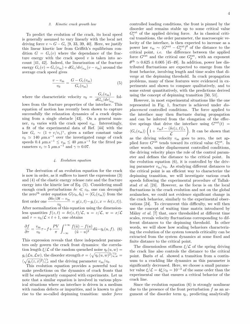
3. Kinetic crack growth law

To predict the evolution of the crack, its local speedis generally assumed to vary linearly with the local netdriving force v ∼ G−Gc [9, 33, 39, 40]. Here, we justifythis linear kinetic law from Griffith’s equilibrium con-dition G = Gc(v) where the dependance of the frac-ture energy with the crack speed v is taken into ac-count [41, 42]. Indeed, the linearization of the fractureenergy Gc(v) = Gc(vm) + dGc/dv|vm(v− vm) around theaverage crack speed gives

v − vmv0

=G−Gc(vm)

Gc(vm)(5)

where the characteristic velocity v0 =Gc(vm)

dGc/dv|vmfol-

lows from the fracture properties of the interface. Thisequation of motion has recently been shown to capturesuccessfully the relaxation dynamics of a crack depin-ning from a single obstacle [43]. On a general man-ner, v0 varies with the crack speed vm. Interestingly,a fit of the experimental data of Ref. [44] with thelaw Gc ∼ (1 + v/vc)

γ , gives a rather constant valuev0 ' 140 µm.s−1 over the investigated range of crackspeeds 0.4 µm.s−1 ≤ vm ≤ 40 µm.s−1 for the fitted pa-rameters vc ' 5 µm.s−1 and γ ' 0.07.

4. Evolution equation

The derivation of an evolution equation for the crackis now in order, as it suffices to insert the expressions (3)and (4) of the elastic energy release rate and the fractureenergy into the kinetic law of Eq. (5). Considering smallenough crack perturbations δc � c0, one can decouplethe zeroth order equation G(c0, δ0) = 〈Gc(vm)〉 from the

first order one∂δc/∂t− vm

v0= g(z, t)−gc(z, x = δc(z, t)).

After normalization of this equation using the dimension-less quantities f(z, t) = δc(z, t)/L, u = z/L, w = x/Land τ = v0/L × t+ 1, one obtains

∂f

∂τ=vmv0τ−f+

PV

π

∫ +∞

−∞

f(u)− f(u)

(u− u)2du−ηc(u, f). (6)

This expression reveals that three independent parame-ters only govern the crack front dynamics: the correla-tion length ξ/L of the random quenched noise ηc(u,w) =

gc(Lu,Lw), the disorder strength σ = 〈√ηc(u,w)2〉1/2u,w =

〈√gc(z, x)2〉1/2z,x and the driving parameter vm/v0.

This evolution equation provides a powerful tool tomake predictions on the dynamics of crack fronts thatwill be subsequently compared with experiments. Let usnote that a similar equation is involved in various phys-ical situations where an interface is driven in a mediumwith random defects or impurities, and is known to giverise to the so-called depinning transition: under force

controlled loading conditions, the front is pinned by thedisorder and remains stable up to some critical valueGext

c of the applied driving force. As in classical criti-cal transitions, the order parameter, the macroscopic ve-locity of the interface, is then expected to increase as apower law vm ∼ (Gext − Gext

c )θ of the distance to thecritical point, i.e. the difference between the appliedforce Gext and the critical one Gext

p , with an exponent

θth ' 0.625 ± 0.005 [45–49]. In addition, power law dis-tributed fluctuations are expected to emerge from thefront behavior, involving length and time scales that di-verge at the depinning threshold. In crack propagationproblems, many of these features were evidenced in ex-periments and shown to compare qualitatively, and tosome extent quantitatively, with the predictions derivedusing the concept of depinning transition [50, 51].

However, in most experimental situations like the onerepresented in Fig. 1, fracture is achieved under dis-placement controlled conditions. The force applied tothe interface may then fluctuate during propagationand can be inferred from the elongation of the effec-tive springs that drive the interface using Gext(t) =

〈Gc(vm)〉(

1 +vmt− 〈δc(z, t)〉z

L

). It can be shown that

as the driving velocity vm goes to zero, the net ap-plied force Gext tends toward its critical value Gext

c . Inother words, under displacement controlled conditions,the driving velocity plays the role of the control param-eter and defines the distance to the critical point. Inthe evolution equation (6), it is controlled by the driv-ing parameter vm/v0. As studying different distances tothe critical point is an efficient way to characterize thedepinning transition, we will investigate various crackspeeds following the experimental procedure of Tallak-stad et al. [24]. However, as the focus is on the localfluctuations in the crack evolution and not on the globalavalanches, we could not evidence significant change inthe crack behavior, similarly to the experimental obser-vations [24]. To circumvent this difficulty, we will thenuse the concept of waiting time matrix introduced byMaløy et al. [7] that, once thresholded at different timescales, reveals velocity fluctuations corresponding to dif-ferent distances to the depinning threshold. In otherwords, we will show how scaling behaviors characteriz-ing the evolution of the system towards criticality can beextracted from the system dynamics at some fixed andfinite distance to the critical point.

The dimensionless stiffness ξ/L of the spring drivingthe crack line also controls the distance to the criticalpoint. Bares et al. showed a transition from a contin-uum to a crackling like dynamics as this parameter issignificantly decreased. Here, we choose a small parame-ter value ξ/L = 4ξ/c0 = 10−3 of the same order than theexperimental one that ensures a critical behavior of thecrack line.

Since the evolution equation (6) is strongly nonlineardue to the presence of the front perturbation f as an ar-gument of the disorder term ηc, predicting analytically

5

the detailed statistical properties of the crack dynamicsremains a very challenging task (see for example Ref. [52]for a review of the appropriate analytical methods basedon the Functional Renormalization Group (FRG) the-ory). In addition, analycal treatments provide only ap-proximated solutions, strictly valid at the critical dimen-sion dc, where d is the interface dimension with dc = 2and d = 1 for crack propagation problems. As a result,we choose to solve the evolution equation (6) numericallyfollowing the procedure described in the next section, andto compare our results with the FRG predictions andother numerical findings when possible.

B. Numerical resolution of the evolution equation

To predict the crack line dynamics, we focus on thedimensionless evolution equation (6) and follow the nu-merical procedure used by Bonamy et al. [9]. The crackfront position is discretized over Nz points with posi-tion ui = ui/L = Lz/L × i/Nz for 1 ≤ i ≤ Nz whereLz = Nz × ξ is the front length along the z-axis. Asa result, at a given time τ , the front configuration isdescribed by the Nz values {f1(τ), f2(τ), . . . , fNz(τ)}.We impose periodic boundary conditions along thez-axis, so that a front of 2Nz points with fbc ={fNz/2+1, . . . , fNz

, f1, . . . , fNz, f1, . . . , fNz/2} is actually

considered for the sake of the numerical calculation. Us-ing this discretization, the evolution equation leads to Nz

linear equations:

fi(τ+δτ) = fi(τ)+δτ×[Gi(f1(τ)...fNz(τ))−ηc(ui, fi(τ))]

(7)with 1 ≤ i ≤ Nz where the unknown are the

f1≤i≤Nz’s and the driving force is given by Gi =

vmv0τ −

fi(τ) +PV

π

∫ fi(τ)+Lz/L

fi(τ)−Lz/L

fbc(u, τ)− fi(τ)

(u− ui)2du. This ex-

plicit scheme allows for the rapid calculation of the frontposition at time τ+δτ from its position at time τ , so thatlarge systems of size Nz = 5000 could be investigated.

The disordered field ηc(ui, wi) that describes the lo-cal resistance to failure is discretized on a square grid(1 : Nz)× (1 : Nz) where the elementary steps are of sizeξ/L. The value of ηc in each node is drawn from a Gaus-sian distribution with unit standard deviation and zeromean value. The value of the toughness at the actual lo-cation of the front {ui, wi = f(ui, τ)} is extrapolated fromthe toughness value of the two neighboring nodes of sameabscissa ui. The physical discretization step along thefront direction is kept equal to the heterogeneity size ξ.This choice is motivated by our interest in the propertiesof the front at scales larger than the disorder correlationlength ξ. At smaller scales, the front dynamics might begoverned by failure processes like e.g. microcracking thatare not taken into account in our model. The effect ofsuch a damage percolation process on the crack dynamicshas recently been studied through an alternative compu-tational fracture model [53] and the comparison of their

results with our predictions will be used in the discussionsection to interpret the experimental observations.

The crack evolution is calculated incrementally bystarting from a straight crack front at time τ = 0 andthen computing f(τ + δτ) from the geometry f(τ) ofthe front at time τ using Eq. (7). We can then comeback to the quantities of interest in physical units likethe crack length δc or the time t by multiplication by thenormalization constants ξ and L/v0. The front positionis calculated over a large number of time steps, typicallya million, that corresponds to a propagation distanceLx = Nx ξ of about Nx = 100 ξ heterogeneity sizes. Thisdistance is several times larger than the one crossed bythe crack during the experiments of Tallakstad et al. [24],as we want to ensure an accurate determination of thecrack statistical features through a large sampling. How-ever, the propagation distance δc(z, τ+δτ)−δc(z, τ)� ξbetween each time step remains small for any position z,ensuring the convergence of our numerical scheme. Forthe post-analysis, only 10% of the computed profiles arekept. This corresponds to about Nt ' 10000 crack po-sitions that are separated by the time step ∆τ . ∆τ issmall enough to ensure that the front spent at least onetime step on each pixel of the grid. This choice takesinspiration from the experimental procedure where theacquisition rate of the camera is set so that the waitingtime matrix that counts the time spent by the front inevery pixel does not contain any zeros. Finally, the tran-sient regime where the front geometry keeps memory ofthe initial straight condition is systematically removedfor the post-treatment. This zone extends over a fewtenths of heterogeneity size in the propagation direction.

For each numerical simulation, we extract three quan-tities that will be used later for the statistical character-ization of the front dynamics:

• The spatio-temporal evolution of the front is storedin the matrix (fi(τj))1≤i≤Nz,1≤j≤Nt

.

• The local velocity of the crack front is stored inthe matrix

(vfronti,j

)1≤i≤Nz,1≤j≤Nt−1

where vfronti,j =

v0fi(τj + ∆τ)− fi(τj)

∆τ. The driving velocity sets

the average front velocity 〈vfronti,j 〉i,j = vm.

• The time spent by the front in each pixel (zi,xi) of the grid is stored in the so-called waitingtime matrix (wi,j)1≤i≤Nz,1≤j≤Nx

. This quantity

has been introduced in Ref. [30] to characterize theavalanche dynamics of the crack front. From it,we define the velocity matrix (vi,j)1≤i≤Nz,1≤j≤Nx

where vi,j = 1/wi,j . This quantity is different fromthe front velocity vfronti,j introduced previously, eventhought a relationship can be established betweentheir probability density function [24].

Following the experimental procedure, we performedsimulations at four different imposed velocities ranging in5×10−4 ≤ vm/v0 ≤ 2.5×10−2. The relevant parameters

6

vm/v0 ∆τ ∆x/ξ Nt Lx/ξ

5.0× 10−4 1.0× 10−2 5× 10−3 20 000 100

2.5× 10−3 3.2× 10−3 8× 10−3 10 000 80

5.0× 10−3 1.6× 10−3 8× 10−3 10 000 80

2.5× 10−2 3.2× 10−4 8× 10−3 10 000 80

TABLE I: Numerical parameters and loading conditions usedfor each simulation: imposed driving velocity vm normalizedby the characteristic velocity introduced in Sec. II A 3, timestep ∆τ between two successive recorded front positions, aver-age distance ∆x crossed during the time step ∆τ , total num-ber Nt of recorded profiles and distance Lx crossed duringthe whole simulation expressed in heterogeneity size ξ. Forall the simulations, the structural length L = 1000 ξ and thedisorder strength σ = 1 are kept the same.

corresponding to each velocity are listed in Table I. Thisrange corresponds about to the smallest crack speeds in-vestigated by Tallakstad et al. [24], as the experimentalrange is 2 × 10−4 . vm/v0 . 1 where the character-istic velocity v0 ' 140 µm.s−1 has been estimated inSec. II A 3. In particular, it includes the specific exper-iment used to investigate the local avalanche statisticsthat corresponds to vm ' 1 × 10−2 v0 [24] and that wewill use in the following.

III. STATISTICAL CHARACTERIZATION OFTHE CRACK EVOLUTION

In this section, we compare the statistical propertiesof the crack front predicted by the depinning model withthe experimental observations. We first study the geo-metrical properties of the crack front through the scal-ing properties of its roughness. Then, we move to thedynamical properties and investigate the correlations be-tween local front velocities, the size distribution of localavalanches and finally the crack speed distribution.

A. Height correlations

Spatial variations of the local resistance result in geo-metrical perturbations of the crack front that we studyhere. The computed crack evolution provides the dimen-sionless front fluctuations δf(u, τ) = f(u, τ) − vm/v0 τwith respect to the mean drift, and hence the physicalfluctuations δc(z, t) = f(z, t)− vm t, from which we com-pute the auto-correlation functions

10−1 100 101 102 10310−1

100

101

!x/"

!xc/

"

100 101 102 103 104

100

101

!zc/

"

!z/"

FIG. 2: Correlation functions of the geometrical pertur-bations of the crack front for the driving velocity vm =5.0 × 10−4 v0. We observe a self-affine behavior both alongthe crack front direction (in inset) and the propagation di-rection (main panel) with exponents ζ ' 0.38 ± 0.02 andβ ' 0.45± 0.05, respectively.

{∆zf(δz) = 〈[δc(z + δz, t)− δc(z, t)]2〉1/2z,t∆xf(δx) = 〈[δc(z, t+ δx/vm)− δc(z, t)]2〉1/2z,t

(8)

These correlations are investigated in Fig. 2 along thecrack front and the propagation direction. We observepower law behaviors

{∆zf(δz) ∝ δzζ∆xf(δx) ∝ δxβ (9)

with exponents ζ = 0.38 ± 0.02 and β = 0.45 ± 0.05.This result is consistent with the theoretical and numer-ical predictions for an elastic line with long-range elas-ticity driven in a disordered medium both for the rough-ness exponent ζth ' 0.388 [18, 54–57] and the so-calledgrowth exponent βth ' 0.495 [49, 54, 55]. The value ofthe roughness exponent is also consistent with the exper-imental value ζexp ' 0.35± 0.05 measured at large scalesfrom images of the crack front as it propagates betweenthe two Plexiglas plates [21].

The growth exponent, classically measured from thetransient roughening of the interface from an initialstraight front condition [58], can also be measured inthe stationary regime by computing the auto-correlationfunction of Eq. (8) in the propagation direction [8, 59].In our simulations, we use the smallest driving velocityvm = 5× 10−4 v0 that turned out to give a reliable mea-surement β ' 0.45. It is found to take a larger value thanthe roughness exponent, in agreement with the theoreti-cal predictions of depinning model and the experimentalvalues βexp ' 0.5− 0.55 [4, 24].

7

B. Velocity correlations

In the strong pinning regime, the motion of the crackis characterized by an alternation of stick periods dur-ing which the front is at rest with slip periods calledavalanches corresponding to the rapid advance of someregions of the front [4, 9, 31]. The spatial structure of atypical avalanche as obtained in the crack growth simu-lation of Laurson et al. [31] is shown in Fig. 3. A strikingfeature is that the region crossed by the crack during anavalanche is not compact, but instead composed of sev-eral clusters. This complex morphology results from thelong-range elasticity of the crack line described by theintegral term in the expression (1) of the elastic energyrelease rate: an advance of the crack somewhere alongthe front results in a redistribution of the driving forcein an extended region. This may trigger the detachmentof some parts of the crack line that are not in the closevicinity of the initiation zone of the avalanche.

x/!

z/!

30

15

000 300 600

!av

"x

FIG. 3: Spatial structure of a typical avalanche as observedduring the simulation of the propagation of a crack in a dis-ordered material for a vanishing front velocity vm → 0 (Cour-tesy of Laurson et al. [31]). ξav and ` represent the lateral sizealong z of the avalanche and its largest cluster, respectively.Their corresponding depth along the propagation directionare noted ξav,x and `x.

The correlations between the local crack speed at dif-ferent times may provide insights on this process, as weexpect velocities corresponding to the same avalanche tobe correlated. As a result, we seek in this paragraph tocharacterize the temporal correlation of the velocity fluc-tuations defined as δvfront(z, t) = vfront(z, t) − vm thatwe compare subsequently with the experimental obser-vations. Our approach consists in exploring how the ve-locity fluctuation at time t correlates with the velocityfluctuation at time t+ δt for a fixed position z along thefront. The correlation function

C(δt) =〈δvfront(z, t+ δt)× δvfront(z, t)〉z,t

〈δvfront(z, t)2〉z,t. (10)

is thus computed for the four velocities vm investigatedand represented in Fig. 4. They all show an exponentialdecay with a characteristic time δt? that decrease withvm, as shown in inset. We observe in fact that δt? isinversely proportional to vm, and hence

C(δt) ' e−δt/δt∗ with δt? ' l0vm

(11)

where l0 ≈ 0.2 ξ. This behavior is in excellent agreementwith the experimental observations of Ref. [24] where asimilar variation of the velocity correlation function withl0 ≈ 0.1× ξ were reported.

How to interpret this remarkable property? As re-minded in Sec. II A 4, the driving velocity controls thedistance to the critical point in the depinning transi-tion. Therefore, as vm decreases, the size and durationof the largest avalanches increase, and in particular theirdepth ξav,x. To relate ξav,x to vm, we predict first the

scaling of the avalanche lateral extent ξav ∼ v−ν/θm us-

ing the definition of the velocity exponent θ remindedin Sec. II A 4 and the correlation length exponent ν thatdescribes the divergence ξav = (Gexp − Gext

c )−ν of theavalanche size close to the depinning threshold. The

avalanche depth ξav,x ∼ ξζav ∼ v−ζ ν/θm then follows us-

ing the roughness exponent ζ that characterizes not onlythe crack roughness (see Sec. III A), but also the as-pect ratio of avalanches [58]. We can then determine

the time δt? = ξav,x/v0 ∼ v−ζ ν/θm required to the front

to cross the largest cluster that corresponds to the cor-relation time of the velocity fluctuations. The predictedexponent takes the simplified form ζ ν/θ = β/(1 − β)after using the scaling relation θ = ν(z − ζ) [60] thatinvolves the dynamic exponent z = ζ/β. It takes avalue βth/(1 − βth) ' 0.98 ± 0.02 close to unity usingthe numerically determined value of the growth exponentβth ' 0.495± 0.005 [49].

Two important assumptions have been made here.First, the depth of the largest cluster has been approxi-mated by the depth of the total avalanche. According tothe numerical observation of Fig. 3, this looks like a fairassumption that relies on the anisotropic spatial struc-ture of the avalanches that extend along the front direc-tion rather than along the propagation direction. Second,we have assumed that the velocity during the propaga-tion of the crack over one cluster is set by the velocityv0, as observed during the depinning from a single ob-stacle [43]. This must not be confused with the typicalcrack velocity ξav,x/ξ

z ∼ vm during the whole avalanchethat scales linearly with the average speed.

This last observation has an interesting consequence,as the macroscopic distance crossed by the crack over thecharacteristic time scale δt? follows δx? = vm δt

? ' l0that is very small compared to the heterogeneity size ξ(see Eq. (11)). This implies that the local front velocitiesalong the propagation direction are essentially uncorre-lated if one investigate two successive positions separatedof at least δx? ' l0 � ξ. As noticed by Tallakstad etal. [24], this implies that the height fluctuations of thefront along the propagation direction follow a randomwalk with exponent β = 1/2. This provides a simple in-terpretation of the numerically determined value of thegrowth exponent β ' 0.495 ± 0.005 [49]. Note that thisproperty is specific to long-range elasticity, as short rangedepinning models exhibit a divergence of the characteris-tic distance δx? in the limit of small driving velocity, and

8

so non-trivial values of the growth exponent β 6= 1/2.

0 200 400 600 800 10000

0.1

0.2

0.3

0.4

0.5

0.6

0.7

0.8

0.9

1

!t ! v0/"

C(!t)

vr/v0 = 5.0 ! 10"4

vr/v0 = 2.5 ! 10"3

vr/v0 = 5.0 ! 10"3

vr/v0 = 2.5 ! 10"2

10−4 10−3 10−2 10−1

101

102

103

vm/v0!t!

!v0/"

FIG. 4: Correlations between the velocity fluctuations at timet and at time t + δt for a fixed position z along the front,as defined in Eq. (10). It shows an exponential decay over acharacteristic time δ? that is represented in inset as a functionof the driving velocity vm.

To summarize, the divergence of the characteristic timeδt? ∼ 1/vm emerging from the velocity fluctuations inour simulations and in the experiments of Tallakstad etal. [24] is signature that the crack is brought closer tothe critical depinning transition as the driving velocityvanishes.

C. Statistics of pinning and depinning clusters

We now go further in the characterization of theavalanche dynamics of the fracture front by exploringthe size distribution of the depinning clusters shown inFig. 3. Inspired by Tallakstad et al. [24], we also studythe size distribution of pinning clusters that reflect thepinned configurations of the front during the stick phases.To study both type of clusters, we apply the procedureproposed by Maløy et al. [30]: We start from the waitingtime matrix defined in Sec. II B that provides the timespent by the crack front on each pixel of the grid. Theinversion of each individual element of this matrix givesthe so-called velocity matrix V that is then thresholdedfollowing the procedure

• depinning regime

V thresd =

{1 if vi,j ≥ C vm0 if vi,j < C vm

• pinning regime

V thresp =

{1 if vi,j ≤ vm/C0 if vi,j > vm/C

This procedure reveals both pinning and depinning clus-ters. Typical thresholded velocity matrices correspond-ing to vm = 5× 10−4v0 are represented in Fig. 5 in bothregimes. The white regions, representing about 35% ofthe total area, correspond to unity while black ones cor-respond to zero. These maps ave been obtained using athreshold value C = 0.6 for depinning and C = 10 forpinning. Note that both figures correspond to the samefractured area of 40 ξ×1000 ξ that represents only a por-tion of the total domain 100 ξ×5000 ξ actually computedand used for the following post-analysis. These clustermaps look qualitatively similar to the experimental onesshown in Fig. 9 of Ref. [24]. Note however two impor-tant differences: The computed maps are about ten timeslarger than the experiment ones after normalizing thedistances by the heterogeneity size ξ. Note also that thespatial resolution of the experimental maps is about tentimes smaller than ξ, while the computed map is resolveduntil ξ. This may explain why the depinning clusters looksomehow bigger in the experiments. We now proceed toa quantitative comparison between the experimental andcomputed cluster maps.

We focus in the following on the slowest driving veloc-ity vm = 5× 10−4v0. The depinning clusters are definedfrom the depinning cluster map from the domains of con-nected pixels for which the local velocity is greater thanthe threshold Cvm. They can be clearly identified onthe depinning threshold velocity matrix of Fig. 5. Simi-larly, the pinning clusters are defined from the domainsof connected pixels for which the local velocity is lowerthan the threshold vm/C. Each of these clusters is char-acterized by several quantities: their width `z along thecrack front direction, their depth `x along the propaga-tion direction and their size S corresponding to the totalarea of the cluster. The statistical distribution of thesequantities is now used to quantify the intermittent crackdynamics and compare the simulation results with theexperiments.

Figure 6 shows the size distribution of pinning anddepinning clusters for different values of the threshold C.We describe their variations with a power law with anexponential cut-off P (Sd) ∼ Sγdd e−Sd/S

?d with S?d ∼ C−σd

P (Sp) ∼ Sγpp e−Sp/S?p with S?p ∼ C−σp .

(12)

in both regimes and determine the values of the expo-nents γ and σ by optimizing the collapse of distributionswith different C values on a same master curve. Thisprocedure gives the exponents γd = 1.55 ± 0.05 for thedepinning clusters and γp = 1.65 ± 0.10 for the pinningclusters. The behavior of Eq. (12) and the value of theseexponents are compatible with the experiments whereγexpd ' γexpp ' 1.56 ± 0.04 were measured [24]. It is alsoconsistent with the results of Laurson et al. [31] who mea-sured γd = 1.53±0.05 through an independent numericalapproach. Finally, it is compatible with the theoreticalprediction γthd ' 1.56 obtained from the scaling relation

9

x/!

x/!

z/!

z/!

Depinning clusters

Pinning clusters

FIG. 5: Representation of the threshold velocity matrices V thresd and V thres

p . For the depinning case, relatively large areasrepresented in white correspond to rapid advances of the front, while for the pinning case, the rather thin lines corresponds tofront position at arrest for some time.

γthd = 2τ − 1 [31] using the global avalanche exponentτ th = 2− 1/(1− ζth) ' 1.28 [35, 61].

Interestingly, the exponents σd = 3.8 ± 0.2 and σp =1.3 ± 0.1 predicted by our simulations that characterizethe variations of the cut-off sizes S?d and S?p with thethreshold C do not match the experimental values σd =1.77± 0.16 and σexp

p = 2.81± 0.23.To confirm this discrepancy, we propose to determine

the predicted values of σd and σp through an indepen-dent method that will also shed light on their physicalsignificance. We follow the idea of [24], and compute inFig. 7 the number of depinning and pinning clusters asa function of the threshold C. They show the followingbehaviors Nd ∼ Cχd with χd ' 1.7± 0.2

Np ∼ Cχp ∼ N0 with χp ' 0.

(13)

We compute then the total area covered by the depinningand pinning clusters as a function of the threshold C. Asshown in Fig. 8, they vary as Ad ∼ − log(C)

Ap ∼ C−κp with κp = 0.42± 0.03

(14)

The logarithmic variations of Ad with C indicates anexponent value κd = 0 if one seeks to characterize thescaling relation Ad ∼ C−κd . The ratio of the area coveredby the clusters over their total number gives the averagecluster size

〈Sd〉 = Nd/Ad and 〈Sp〉 = Np/Ap. (15)

The latter can be related to the threshold C fromthe integrals 〈Sd〉 =

∫∞0Sd P (Sd) dSd and 〈Sp〉 =∫∞

0Sp P (Sp) dSp of the cluster size distributions of

Eq. (12). This gives the following scaling relations 〈Sd〉 = (S?d)2−γd ∼ C−σd(2−γd)

〈Sp〉 =(S?p)2−γp ∼ C−σp(2−γp).

(16)

We can now introduce the scaling laws (13), (14) and (16)in Eq. (15) to relate these exponents together through κd = σd(2− γd)− χd

κp = σp(2− γp)− χp.

(17)

These expressions simplify to σd = χd/(2− γd)

σp = κp/(2− γp)

(18)

after taking into account that both κd and χp are equalto zero. These last relations provide independent esti-mates of the exponents σd ' 3.8 and σp ' 1.2 that are ingood agreement with their estimation made in Fig. 6 fromthe collapse of the cluster size distributions computed atdifferent threshold values. And at the same time, it con-firms the gap between the numerically determined andexperimentally measured value of both exponents.

Before getting to the origin of this discrepancy, weprovide some insights on the physical meaning of theexponent σd and a possible interpretation of its valueas measured in our simulations. Consider the size S∗avof the largest avalanches as we drive the crack at fi-nite but small velocity vm. It follows S∗av ∼ ξ1+ζ whereξ is the correlation length along the crack line. Since

the correlation length diverges as ξ ∼ v−ν/θm when the

driving velocity vanishes, the typical size of the largestavalanches digerges too, following the scaling behavior

S?av ∼ v−σav

dm ∼ v

−(1+ζ) ν/θm . From the relations be-

tween critical exponents already used in Sec. III B, oneobtains σav

r = (1/ζ + 1)/(1/β − 1) that simplifies toσavd = 1 + 1/ζ ' 3.58 ± 0.02 after using β = 1/2 de-

termined previously and the value of the roughness ex-ponent ζ ' 0.388 [57]. This value is surprisingly closeof the exponent σd ' 3.8 that characterizes the varia-tions of cut-off cluster size when the velocity matrix isthresholded at different levels C vm.

10

10−1 100 101 102 10310−8

10−6

10−4

10−2

100

102

Sd C!d

P/C

!d"d

C = 0.4

C = 0.6

C = 0.8

C = 1.0

C = 1.2

C = 1.4

Fit: "d = 1.55

103 104 105 10610−12

10−10

10−8

10−6

10−4

Sp C!p

P/C

!p"p

C = 20

C = 30

C = 40

C = 50

C = 60

C = 80

C = 100

C = 120

Fit: "p = 1.65

FIG. 6: Normalized distributions of sizes of depinning clusters(upper panel) and pinning clusters (lower panel) for variousvalues of the threshold C. Both families of distributions arewell described by the power law behavior of Eq. (12) withexponents γd = 1.55 ± 0.05 and γp = 1.65 ± 0.10 that arecompatible with the experimental findings [24]. On the con-trary, the scaling of the cut-offs S∗

d ∼ C−σd and S∗p ∼ C−σp

lead to σd = 3.8 ± 0.2 and σp = 1.3 ± 0.1, in disagreementwith the values measured experimentally.

This observation calls for the following comment: inour analysis, we considered a fixed velocity vm of thefront, and characterized the distribution of depinningclusters defined from the regions where the local veloc-ity was larger than vthres = C vm. We observed that thesmaller the threshold, the larger the size of the depin-ning clusters, and we could evidence the following scal-ing S?d ∼ v−σd

thres. We believe that this procedure revealsthe depinning clusters as they would be observed if thedriving velocity was actually equal to vthres. From thispostulate, σd and σav

d are then the very same exponentas they both characterize the divergence of the size of thelargest depinning cluster or avalanche when the drivingvelocity goes to zero. Note that we need to assume herethat the largest avalanche size S∗av is proportional to thelargest cluster size S∗d. This was indeed observed by Laur-son et al. [31] who found Sd ∼ Sav for the largest events.

10−2 10−1 100 101 102101

102

103

104

105

C

Ncluster

Fit: !d = 1.7

Depinning clusters

Pinning clusters

Fit: !p = 0

FIG. 7: Variations of the number of depinning and pinningclusters with the threshold C.

100 101 102

10−1

100

C

Ap

10−1 100 1010

0.20.40.60.81

Ad

C

Fit: ! d = 0

Depinn ingc lusters

Pinning clusters

Fit: !p = 0.42

FIG. 8: Area covered by the pinning and the depinnning clus-ters on the activity maps of Fig. 5 normalized by the total areacrossed by the crack.

Overall, our result suggests an interesting method forthe analysis of depinning transition: scaling relations de-picting the divergence of quantities of interest with thedistance to the critical point can be determined with-out performing several experiments or simulations at dif-ferent driving velocities. Indeed, they can be achievedfrom a single study performed at some fixed velocity vmthrough the thresholding of the obtained velocity field atdifferent levels vthres = C vm and the scaling behavior interms of vthres.

D. Distribution of crack velocities

We now move to the study of the distribution p(v) oflocal crack speeds. We consider the velocity values storedin the velocity matrix V and compute their probabilitydensity function that is shown in Fig. 9. It shows two

11

10−2 10−1 100 101100

101

102

v/vm

p

Pinning regime

Fit: !p = 1.6

Depinning regime

Fit: !d = 2.0

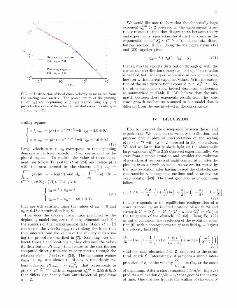
FIG. 9: Distribution of local crack velocity as measured fromthe waiting time matrix. The power law fit of the pinning(v � vm) and depinning (v & vm) regime using Eq. (19)provides the value of the velocity distribution exponents ηp =1.6 and ηp = 2.0.

scaling regimes v & vm ⇒ p(v) ∼ v−(ηd−1) with ηd = 2.0± 0.1

v � vm ⇒ p(v) ∼ v−(ηp−1) with ηp = 1.6± 0.1.(19)

Large velocities v > vm correspond to the depinningdomains while lower speeds v < vm correspond to thepinned regions. To confirm the value of these expo-nent, we follow Tallakstad et al. [24] and relate p(v)with the area covered by the clusters using Ad =∫ vmax

Cvm

p(v)dv ∼ − log(C) and Ap =

∫ vm/C

0

p(v)dv ∼

C−κp (see Eqs. (14)). This gives ηd = 2 + κd = 2

ηp = 2− κp ' 1.58± 0.03

(20)

that are well satisfied using the values of κd = 0 andκp ' 0.42 determined in Fig. 8.

How does the velocity distribution predicted by thedepinning model compare to the experimental one? Forthe analysis of their experimental data, Maløy et al. [7]considered the velocity vfront(z, t) along the front thatthey inferred from the values of the velocity matrix us-ing the procedure described in [7]. Sampling over dif-ferent times t and locations z, they obtained the veloc-ity distribution P (vfront) that relates to the distributioncomputed directly from the velocity matrix through therelation p(v) = P (v) v/vm [24]. The depinning regimevfront > vm was shown to display a remarkably ro-

bust behavior P (vfront) ∼ v−ηexpd

front that corresponds to

p(v) ∼ v−(ηexpd −1) with an exponent ηexpd = 2.55 ± 0.15

that differs significanly from our theoretical predictionηd = 2.

We would like now to show that the abnormally largeexponent ηexpd > 2 observed in the experiments is ac-tually related to the other disagreement between theoryand experiments reported in this study that concerns theexponential cut-off S?d ∼ C−σd of the cluster size distri-bution (see Sec. III C). Using the scaling relations (17)and (20) together gives

ηd = 2 + σd(2− γd)− χd (21)

that relates the velocity distribution through ηd with thecluster size distribution through σd and γd. This relationis verified both for experiments and in our simulations,however with different exponent values. With the excep-tion of the size distribution exponent σd ' σexp

d ' 1.55,the other exponents show indeed significant differencesas summarized in Table II. We believe that the mis-match between these exponents results from the basiccrack growth mechanism assumed in our model that isdifferent from the one involved in the experiments.

IV. DISCUSSION

How to interpret the discrepancy between theory andexperiment? We focus on the velocity distribution, andpropose first a physical interpretation of the scalingp(v) ∼ v−ηd with ηd = 2 observed in the simulations.We will see later that it sheds light on the abnormallylarge exponent ηexpd ' 2.55 observed experimentally. Westart from a simple situation and consider the evolutionof a crack as it recovers a straight configuration after de-pinning from a single obstacle. As we are interested bythe front evolution after having passed the obstacle, onecan consider a homogenous medium and so achieve anexact solution [43]. The front geometry prior depinningfollows

c(z, t < 0) =C d

π

[(1 +

z

d

)ln∣∣∣1 +

z

d

∣∣∣+(

1− z

d

)ln∣∣∣1− z

d

∣∣∣](22)

that corresponds to the equilibrium configuration of acrack trapped by an isolated obstacle of width 2d andstrength C = (GOc − 〈Gc〉)/〈Gc〉 where GOc > 〈Gc〉 isthe toughness of the obstacle [62, 63]. Using Eq. (22)as initial condition, the resolution of the evolution equa-tion (6) with a homogeneous toughness field ηc = 0 givesthe velocity field [43]

∂c

∂t= Cv0

[1− 1

π

(arctan

(v0 t

d+ z

)+ arctan

(v0 t

d− z

))](23)

valid for small obstacles d � L compared to the struc-tural length L. Interestingly, it provides a simple inter-

pretation of v0 as the velocity∂c

∂t

∣∣∣∣z,0

= Cv0 at the onset

of depinning. After a short transient t� d/v0, Eq. (23)predicts a relaxation ∂c/∂t ∼ 1/t that goes as the inverseof time. One deduces from it the scaling of the velocity

12

Depinning γd σd χd κd ηd

Sim. 1.55± 0.05 3.8± 0.2 1.7± 0.2 0 2.0± 0.1

Exp. 1.56± 0.04 1.77± 0.16 0.28 0.5 2.55± 0.15

Pinning γp σp χp κp ηp

Sim. 1.65± 0.10 1.3± 0.1 0 0.42± 0.03 1.60± 0.05

Exp. 1.56± 0.04 2.81± 0.23 ø ø ø

TABLE II: Critical exponents measured numerically in both the depinning and pinning regime, and their comparison with theexperimental values of Refs. [4, 24].

distribution p(v) ∼ 1/v2 during one avalanche resultingfrom the depinning of the front from a single obstacle.Depinning clusters observed during the evolution of thecrack through disordered interfaces result from the de-pinning from several obstacles. However, our simulationsshow that the scaling of the velocity distribution remainsunaffected and also follows P (v) ∼ 1/v2, irrespective ofthe cluster size and the number of obstacles involved inthe depinning process (see Fig. 9). This provides inter-pretation for the statistics P (v) ∼ 1/v2 observed in oursimulations in the depinning regime: It reflects the frontrelaxation between two pinned configurations.

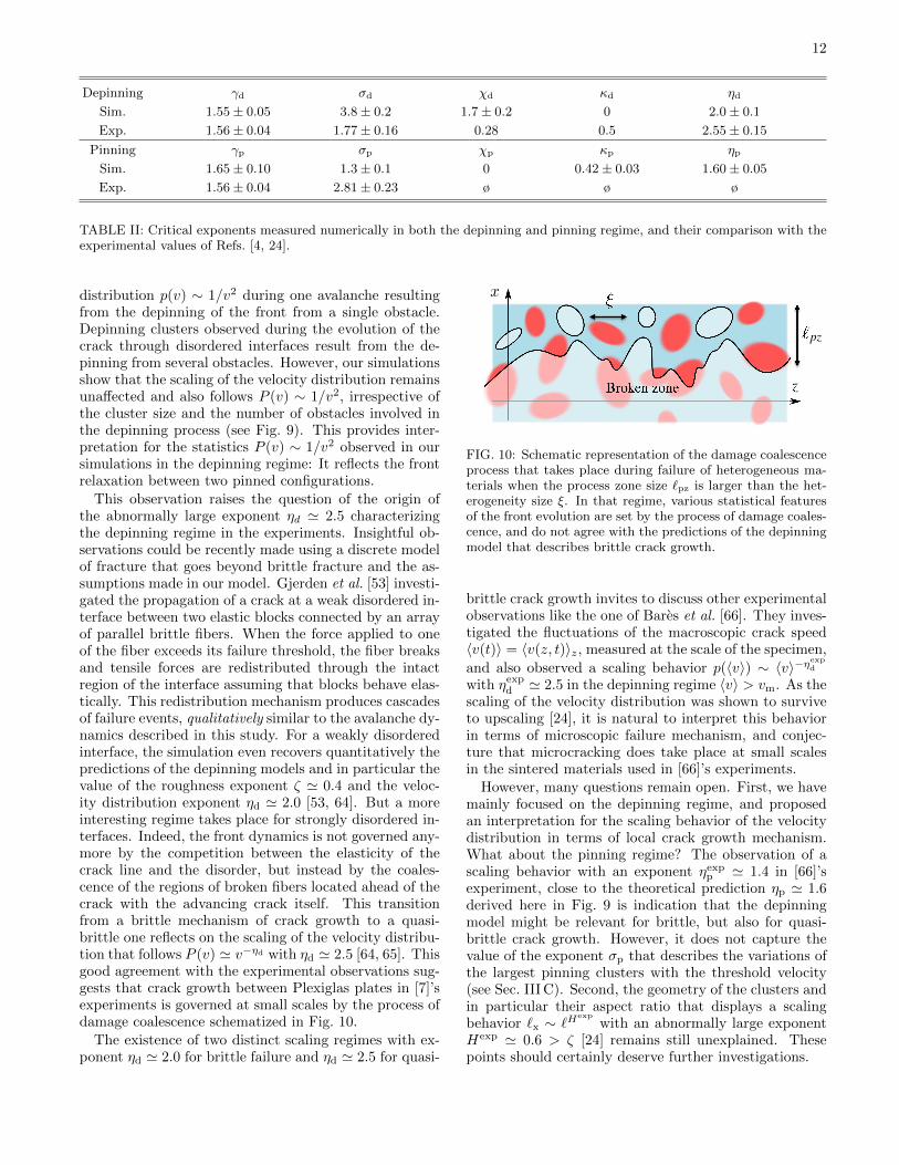
This observation raises the question of the origin ofthe abnormally large exponent ηd ' 2.5 characterizingthe depinning regime in the experiments. Insightful ob-servations could be recently made using a discrete modelof fracture that goes beyond brittle fracture and the as-sumptions made in our model. Gjerden et al. [53] investi-gated the propagation of a crack at a weak disordered in-terface between two elastic blocks connected by an arrayof parallel brittle fibers. When the force applied to oneof the fiber exceeds its failure threshold, the fiber breaksand tensile forces are redistributed through the intactregion of the interface assuming that blocks behave elas-tically. This redistribution mechanism produces cascadesof failure events, qualitatively similar to the avalanche dy-namics described in this study. For a weakly disorderedinterface, the simulation even recovers quantitatively thepredictions of the depinning models and in particular thevalue of the roughness exponent ζ ' 0.4 and the veloc-ity distribution exponent ηd ' 2.0 [53, 64]. But a moreinteresting regime takes place for strongly disordered in-terfaces. Indeed, the front dynamics is not governed any-more by the competition between the elasticity of thecrack line and the disorder, but instead by the coales-cence of the regions of broken fibers located ahead of thecrack with the advancing crack itself. This transitionfrom a brittle mechanism of crack growth to a quasi-brittle one reflects on the scaling of the velocity distribu-tion that follows P (v) ' v−ηd with ηd ' 2.5 [64, 65]. Thisgood agreement with the experimental observations sug-gests that crack growth between Plexiglas plates in [7]’sexperiments is governed at small scales by the process ofdamage coalescence schematized in Fig. 10.

The existence of two distinct scaling regimes with ex-ponent ηd ' 2.0 for brittle failure and ηd ' 2.5 for quasi-

Broken zone z

!pz

"x

FIG. 10: Schematic representation of the damage coalescenceprocess that takes place during failure of heterogeneous ma-terials when the process zone size `pz is larger than the het-erogeneity size ξ. In that regime, various statistical featuresof the front evolution are set by the process of damage coales-cence, and do not agree with the predictions of the depinningmodel that describes brittle crack growth.

brittle crack growth invites to discuss other experimentalobservations like the one of Bares et al. [66]. They inves-tigated the fluctuations of the macroscopic crack speed〈v(t)〉 = 〈v(z, t)〉z, measured at the scale of the specimen,

and also observed a scaling behavior p(〈v〉) ∼ 〈v〉−ηexpd

with ηexpd ' 2.5 in the depinning regime 〈v〉 > vm. As thescaling of the velocity distribution was shown to surviveto upscaling [24], it is natural to interpret this behaviorin terms of microscopic failure mechanism, and conjec-ture that microcracking does take place at small scalesin the sintered materials used in [66]’s experiments.

However, many questions remain open. First, we havemainly focused on the depinning regime, and proposedan interpretation for the scaling behavior of the velocitydistribution in terms of local crack growth mechanism.What about the pinning regime? The observation of ascaling behavior with an exponent ηexpp ' 1.4 in [66]’sexperiment, close to the theoretical prediction ηp ' 1.6derived here in Fig. 9 is indication that the depinningmodel might be relevant for brittle, but also for quasi-brittle crack growth. However, it does not capture thevalue of the exponent σp that describes the variations ofthe largest pinning clusters with the threshold velocity(see Sec. III C). Second, the geometry of the clusters andin particular their aspect ratio that displays a scalingbehavior `x ∼ `H

exp

with an abnormally large exponentHexp ' 0.6 > ζ [24] remains still unexplained. Thesepoints should certainly deserve further investigations.

13

To conclude, we showed that the model of brittle frac-ture proposed in this study that builds on the conceptof depinning transition can be used as a an efficient toolto predict crack evolution in disordered materials. Itssuccess is conditioned to the implementation of two sys-tem specific characteristics, namely (i) the actual frac-ture properties of the material through the characteris-tic velocity v0 and (ii) the specimen geometry throughthe structural length L. However, the few but significantmismatches with some experimental observations suggestthat an ingredient might be missing in the theoretical ap-proach proposed in this work. We proposed that it relatesto the mechanism of damage coalescence that takes place

at small scales within the process zone in some materi-als. Back and forth between experiment and theory willcertainly help to better characterize this mechanism andultimately integrate it into the crack evolution equationproposed in this study.

V. ACKNOWLEDGEMENTS

The authors would like to thank Daniel Bonamy, PierreLe Doussal, Jean-Baptiste Lebond and Alberto Rosso forenlightening discussions.

[1] S. Xia, L. Ponson, G. Ravichandran, and K. Bhat-tacharya, Phys. Rev. Lett. 108, 196101 (2012).

[2] L. S. Dimas, G. H. Bratzel, I. Eylon, and M. Buehler,Adv. Func. Mat. 23, 4629 (2013).

[3] A. Ghatak, Phys. Rev. E 89, 032407 (2014).[4] K. J. Maløy and J. Schmittbuhl, Phys. Rev. Lett. 87,

105502 (2001).[5] S. Santucci, L. Vanel, and S. Ciliberto, Phys. Rev. Lett.

93, 095505 (2004).[6] E. Bouchaud, G. Lapasset, and J. Planes, Europhys.

Lett. 13, 73 (1990).[7] K. J. Maløy, A. Hansen, E. L. Hinrichsen, and S. Roux,

Phys. Rev. Lett. 68, 213 (1992).[8] L. Ponson, D. Bonamy, and E. Bouchaud, Phys. Rev.

Lett. 96, 035506 (2006).[9] D. Bonamy, S. Santucci, and L. Ponson, Phys. Rev. Lett.

101, 045501 (2008).[10] D. Bonamy, L. Ponson, S. Prades, E. Bouchaud, and

C. Guillot, Phys. Rev. Lett. 97, 135504 (2006).[11] L. Ponson and D. Bonamy, Int. J. Frac. 162, 21 (2010).[12] S. Patinet, D. Vandembroucq, and S. Roux, Phys. Rev.

Lett. 110, 165507 (2013).[13] V. Demery, A. Rosso, and L. Ponson, EPL 105, 34003

(2014).[14] E. Rolley and C. Guthmann, Phys. Rev. Lett. 98, 166105

(2007).[15] P. J. Metaxas, J. P. Jamet, A. Mougin, M. Cormier,

J. Ferre, V. Baltz, B. Rodmacq, B. Dieny, and R. L.Stamps, Phys. Rev. Lett. 99, 217208 (2007).

[16] S. Patinet, D. Bonamy, and L. Proville, Phys. Rev. B 84,174101 (2011).

[17] H. Herrmann and S. Roux, Statistical Models for theFracture of Disordered Media (Elsevier, 1990).

[18] J. Schmittbuhl, S. Roux, J. P. Vilotte, and K. J. Maløy,Phys. Rev. Lett. 74, 1787 (1995).

[19] J. P. Bouchaud, E. Bouchaud, G. Lapasset, andJ. Planes, Phys. Rev. Lett. 71, 2240 (1993).

[20] L. Laurson, X. Illa, S. Santucci, K. T. Tallakstad, K. J.Maløy, and M. J. Alava, Nature Com. 4, 2927 (2013).

[21] S. Santucci, M. Grob, R. Toussaint, J. Schmittbuhl,A. Hansen, and K. J. Maløy, EPL 92, 44001 (2010).

[22] J. Koivisto, J. Rosti, and M. J. Alava, Phys. Rev. Lett.99, 145504 (2007).

[23] L. Ponson, Phys. Rev. Lett. 103, 055501 (2009).[24] K. T. Tallakstad, R. Toussaint, S. Santucci, J. Schmit-

tbuhl, and K. J. Maløy, Phys. Rev. E 83, 046108 (2011).[25] J. P. Sethna, K. A. Dahmen, and C. R. Myers, Nature

410, 241 (2001).[26] A. Prevost, E. Rolley, and C. Guthmann, Phys. Rev. B

67, 064517 (2002).[27] F. F. Csikor, C. Motz, D. Weygand, M. Zaiser, and

S. Zapperi, Science 318, 251 (2007).[28] J. Davidsen, S. Stanchits, and G. Dresen, Phys. Rev.

Lett. 98, 125502 (2007).[29] A. Garcimartin, A. Guarino, L. Bellon, and . Ciliberto,

Phys. Rev. Lett. 79, 3203 (1997).[30] K. J. Maløy, S. Santucci, J. Schmittbuhl, and R. Tous-

saint, Phys. Rev. Lett. 96, 045501 (2006).[31] L. Laurson, S. Santucci, and S. Zapperi, Phys. Rev. E

81, 046116 (2010).[32] J. R. Rice, J. Appl. Mech. 52, 571 (1985).[33] H. Gao and J. R. Rice, J. Appl. Mech. 56, 828 (1989).[34] B. Lawn, Fracture of brittle solids (Cambridge University

Press, 1993).[35] A. Rosso, P. Le Doussal, and K. J. Wiese, Phys. Rev. B

80, 144204 (2009).[36] A. A. Middleton, P. Le Doussal, and K. J. Wiese, Phys.

Rev. Lett. 98, 155701 (2007).[37] A. I. Larkin and Y. N. Ovchinnikov, Nonequilibrium su-

perconductivity (Elsevier, Amsterdam, 1989).[38] A. Tanguy and T. Vettorel, Eur. Phys. J. B 38, 71 (2004).[39] S. Ramanathan, D. Ertas, and D. S. Fisher, Phys. Rev.

Lett. 79, 873 (1997).[40] E. Katzav and M. Adda-Bedia, EPL 76, 450 (2006).[41] I. Kolvin, G. Cohen, and J. Fineberg, Phys. Rev. Lett.

114, 175501 (2015).[42] L. Ponson, Int. J. Frac. (in press).[43] J. Chopin, A. Bhaskar, and L. Ponson (in preparation).[44] O. Lengline, R. Toussaint, J. Schmittbuhl, J. E.

Elkhoury, J. P. Ampuero, K. T. Tallakstad, S. Santucci,and K. J. Maløy, Phys. Rev. E 84, 036104 (2011).

[45] M. Kardar, Phys. Reports 301, 85 (1998).[46] D. Ertas and M. Kardar, Phys. Rev. E 49, R2532 (1994).[47] O. Narayan and D. S. Fisher, Phys. Rev. B 48, 7030

(1993).[48] H. Leschhorn, T. Nattermann, S. Stepanow, and L. H.

Tang, Ann. Phys. 6, 1 (1997).[49] O. Duemmer and W. Krauth, J. Stat. Mech. 1, 01019

(2007).[50] D. Bonamy and E. Bouchaud, Phys. Rep. 498, 1 (2011).

14

[51] D. Bonamy, J. Phys. D: Appl. Phys. 42, 214014 (2009).[52] K. Wiese and P. Le Doussal, in Markov processes and

related fields (Polymath, Moscow, 2007), vol. 13, pp. 777–818.

[53] K. S. Gjerden, A. Stormo, and A. Hansen, Phys. Rev.Lett. 111, 135502 (2013).

[54] D. Ertas and M. Kardar, Phys. Rev. Lett. 69, 929 (1992).[55] P.Chauve, P. Le Doussal, and K. J. Wiese, Phys. Rev.

Lett. 86, 1785 (2001).[56] A. Tanguy, M. Gounelle, and S. Roux, Phys. Rev. E 58,

1577 (1998).[57] A. Rosso and W. Krauth, Phys. Rev. Lett. 87, 187002

(2001).[58] A. L. Barabasi and H. E. Stanley, Fractal concepts in

surface growth (Cambridge University Press, 1995).[59] M. Kardar, G. Parisi, and Y.-C. Zhang, Phys. Rev. Lett.

56, 889 (1986).[60] T. Nattermann, S. Stepanow, S. Tang, and H. Leschhorn,

J. Phys. II 2, 1483 (1992).[61] J. Lin, E. Lerner, A. Rosso, and M. Wyart, Proc. Nat.

Acad. Sci. 111, 14382 (2014).[62] J. Chopin, A. Prevost, A. Boudaoud, and M. Adda-

Bedia, Phys. Rev. Lett. 107, 144301 (2011).[63] M. Vasoya, J.-B. Leblond, and L. Ponson, Int. J. Solids

Struct. 50, 371 (2013).[64] A. Stormo, O. Lengline, J. Schmittbuhl, and A. Hansen,

Front. Phys. 4, 18 (2016).[65] K. G. Gjerden, A. Stormo, and A. Hansen, Front. Phys.

2, 66 (2014).[66] J. Bares, L. Barbier, and D. Bonamy, Phys. Rev. Lett.

111, 054301 (2013).

Crack propagation through disordered materials as a...

Documents

Transcript of Crack propagation through disordered materials as a...