cR2 v3.0 readme - es.lancs.ac.uk

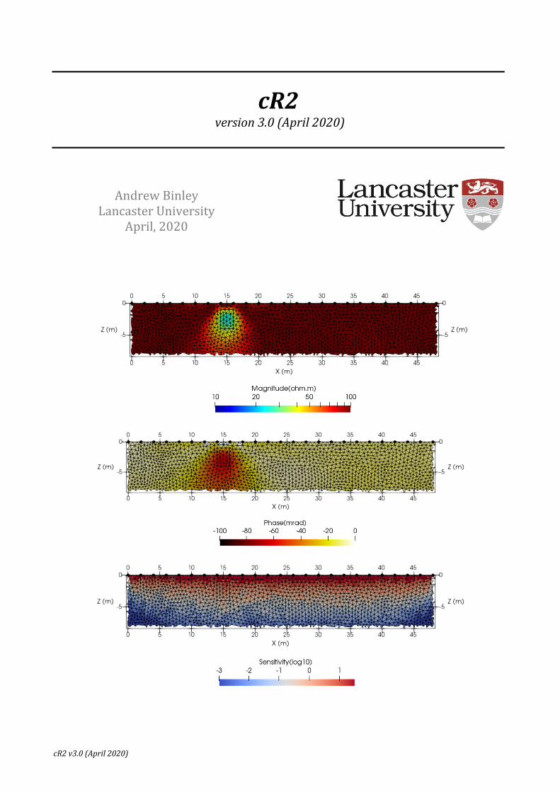
cR2v3.0(April2020)

cR2 version3.0(April2020)

Andrew Binley

Lancaster University April, 2020

cR2v3.0(April2020)

Contents

Page 1. Version history 1 2. Computer requirements for cR2 v3.0 2 3. Introduction to cR2 v3.0 3 4. Designing meshes 5 5. Parameterisation 9 6. Input and output files 12 7. Details of cR2.in 15 8. Details of protocol.dat 21 9. Details of mesh.dat 22 10. Examples 23 11. Additional codes and scripts 33 12. Getting started with ParaView 34 13. Common user errors 35 14. References 37

cR2v3.0(April2020) page1

1. Versionhistory

ChangestocR2fromv2.0 General (unstructured) quadrilateral mesh input now an option. When an unstructured (triangular or quadrilateral) mesh is used the mesh.dat file now needs specification of the Dirichlet node in line 1. Error checking on presence of input files. Mesh error checks when mesh is read from file mesh.dat. Output of model roughness in main log file. Bug fix: geometric factor calculations for triangular meshes. Bug fix: output of electrode codes in the _err.dat file (only has impact if electrode numbers are different to the order they are defined in cR2.in. ChangestocR2fromv1.9 Allocatable (dynamic) arrays are now used, meaning that there is (in theory) no problem size limit. A sensitivity map is now produced (as a separate file and embedded with the vtk). The input of starting resistivity and phase in cR2.in is now consistent with R2v3.2. A bug fix has been corrected that affected calculations with a triangular mesh when node 1 was close to (or at) an electrode (that resulted in high errors in forward model calculations for measurements involving such an electrode). Error checks on input of the data file (protocol.dat) are now made (to avoid incorrect electrode numbering). An option for a more gradual progression of the inversion is now added (consistent with R2v3.2). Documentation has been improved by adding more illustration of meshing and parameterisation. ChangestocR2fromv1.8aVtk output is now created. The output region can also be selected. ChangestocR2fromv1.8An option to output the Jacobian in a forward model is added. ChangestocR2fromv1.7The mesh input is completely changed and now follows a similar format to R2v2.5 Linear solver for forward problem now uses PARDISO solver. This may result in slower execution but much larger problems can be solved. ChangestocR2fromv1.6For a quadrilateral mesh it is now necessary to define the elevations of all electrodes – see line 22 in cR2.in details below. This now allows topographic variation in the mesh.


2. ComputerrequirementsforcR2v3.0

In this release only one version has been compiled for the Windows environment: a 64bit version, cR2.exe. A 32bit version is not provided because of the limited array allocation. Linux users should be able to run cR2 with the command “wine cR2.exe” (thanks to Rodolphe Cattin for this tip). I have not tested this, however. Users requiring a version compiled for other processors should contact the author. NOTE1:cR2isprovidedasastandaloneexecutable.Itdoesnotneedtobeinstalled–theexecutableisputinthefoldercontainingtheinputfilesandrunfromthere.Outputfileswillbecreatedinthesamefolder. NOTE2:YouwillbeabletoruncR2bydoubleclickingtheexecutable.However,iftheprogramstopsabruptly(forexample,duetoanerrorintheinputfileorifyouaretryingtorunanexecutablecompiledforadifferentprocessorarchitecture)thenyouwillnotseeanyerrormessageonthescreensincethewindowwilldisappear.Therefore,itisadvisabletoruncR2fromtheCommandPrompt(justrunCMDfromtheStartMenu–youmayneedtomoveyourworkingdirectoryandruncR2fromthere).NOTE3:allinputfilesshouldbepreparedwithatexteditor.[IprefertouseTextPad(www.textpad.com)becauseitallowsmuchgreatereditingfacilitiesalthoughanytexteditorwillwork].Itisimportantthatyoudonotincludetabsinthefiles.TheseareofteninsertedifyoucopyandpastefromExcel,forexample.Youshouldconvertthesetabstospaces(TextPadwillallowyoutosetthisuptohappenautomatically). cR2 has been designed so that no other commercial software is required for pre- and post-processing. Simple structured meshes can be created directly in cR2, alternatively more complex geometry can be meshed using freely available codes, such as Gmsh (http://www. gmsh.info). cR2 does not produce graphical output but results compatible with the freely available ParaView(https://www.paraview.org) are produced. Other free codes, such as GMT (https://github.com/GenericMappingTools/gmt) can be used. Users wishing to use a graphical user interface for meshing, modelling and plotting may be interested in ResIPy - an open source python GUI for cR2 and sister codes. See https://gitlab.com/hkex/pyr2 which also includes links for standalone executables. More information is also available at https://www.researchgate.net/project/ResIPy-GUI-for-R2-family-codes.


3. IntroductiontocR2v3.0 cR2has been developed for imaging complex resistivity (i.e. induced polarisation) using arbitrary electrode arrays. cR2will compute a forward model for a given distribution of complex resistivity (defined in terms of magnitude and phase angle). cR2 can also provide an inverse solution for a 2-D complex resistivity distribution based on computation of 3-D current flow using a finite element mesh based on either triangle or rectangle elements. The inverse solution is based on a regularised objective function combined with weighted least squares (an ‘Occams’ type solution) as defined in Binley and Kemna (2005) and Kemna etal.(2004). Parameters (for the inverse solution) are made up of one or more elements. Electrodes are specified at node points. These are the corners of the elements. The boundary conditions along all four boundaries of the mesh are Neumann conditions (zero flux) and therefore if you are investigating a half space you must extend left, right and lower boundaries of the mesh to some distance away from the area of investigation (typically 5 to 10 times the distance – see later). The mesh can be made up of either quadrilateral elements or triangular elements. The current version does not have upper limits set for the size of the problem that can be solved. However, it is important that the user has some appreciation of whether the problem they are trying to solve is realistic for their given hardware. Large problems in inverse mode can be memory hungry. As soon as the user’s RAM is used then the computer will start using virtual memory (paging to disk) which can be very slow. To help the user asses memory needs cR2will output an estimate of the memory needs early on in its execution. For large problems it is important that the user compares this with physical memory (RAM) that is available. For information on solving resistivity forward and inverse problems see Binley (2015) and Binley and Kemna (2005), the latter being useful for the full complex resistivity description. Contact the author for a digital copy of the former. It is strongly recommended that the user becomes familiar with inverting DC resistivity data with sister code R2 before working with cR2. Many of the concepts about meshing, parameterisation are similar and the documentation for R2 covers examples that will help the user become familiar with either R2 or cR2. In cR2 complex resistivity is defined by a magnitude and phase angle. The magnitude is equivalent to a DC resistivity since the phase angles are likely to be small. In an inversion, cR2also computes the real and imaginary conductivity since these are more useful for analysis of the conduction and polarization of the subsurface. Data for cR2 are supplied in terms of magnitude and phase angle of the measured impedance. A negative phase angle is a positive IP effect. It is important to understand that the magnitude is a positive number, unlike DC resistance, which can be positive or negative. For example, a surface DC resistivity dipole-dipole survey with four adjacent electrodes, 1,2,3 and 4 in AB-MN configuration 1,2 – 3,4 will give a negative resistance since the geometric factor is negative. Let’s say that the value is -1.0. If a complex resistivity survey is carried out with the same configuration then the magnitude would be 1.0 and the phase angle (for a non-polarizing subsurface) would not be zero but would be – radians, i.e. -3,141.6 mrad. Preparing data in this way can be messy and lead to confusion and so measurements with a negative geometric factor it may be easier to express the measurement as the equivalent with a positive geometric factor. The values below are equivalent.

A B M N Magnitude()

Phaseangle(mrad)

1 2 3 4 1.0 -3,141.6 1 2 4 3 1.0 0.0 2 1 3 4 1.0 0.0


IP data measured in the time domain will give a resistance and chargeability (M). The resistance is easily transformed to a magnitude taking care of the polarity issue above. The chargeability can be transformed to an equivalent phase angle using the method described in Kemna et al. (1997). The conversion is a function of the chargeability sampling and current injection frequency. Typically the phase angle (in mrad) is equivalent to ~-1.3M (in mV/V). See Mwakanyamale et al.(2012) as an example of such a conversion for application of cR2 to time domain IP data.


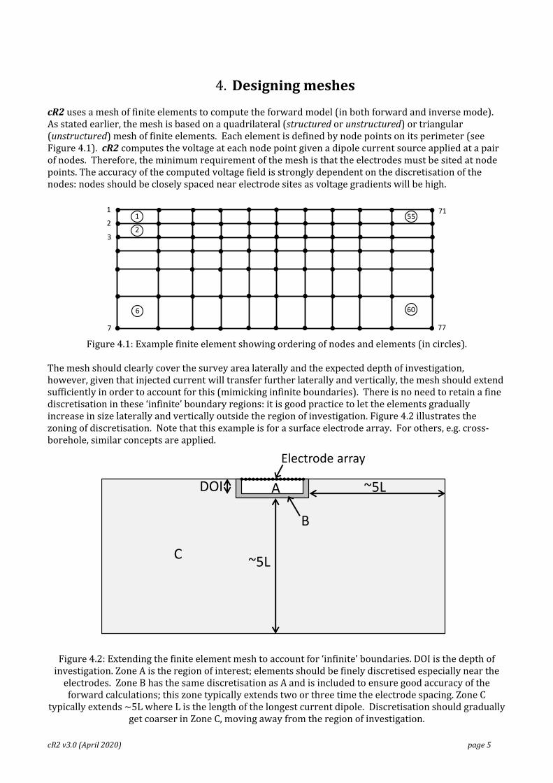
4. Designingmeshes cR2 uses a mesh of finite elements to compute the forward model (in both forward and inverse mode). As stated earlier, the mesh is based on a quadrilateral (structured or unstructured) or triangular (unstructured) mesh of finite elements. Each element is defined by node points on its perimeter (see Figure 4.1). cR2 computes the voltage at each node point given a dipole current source applied at a pair of nodes. Therefore, the minimum requirement of the mesh is that the electrodes must be sited at node points. The accuracy of the computed voltage field is strongly dependent on the discretisation of the nodes: nodes should be closely spaced near electrode sites as voltage gradients will be high.

Figure 4.1: Example finite element showing ordering of nodes and elements (in circles).

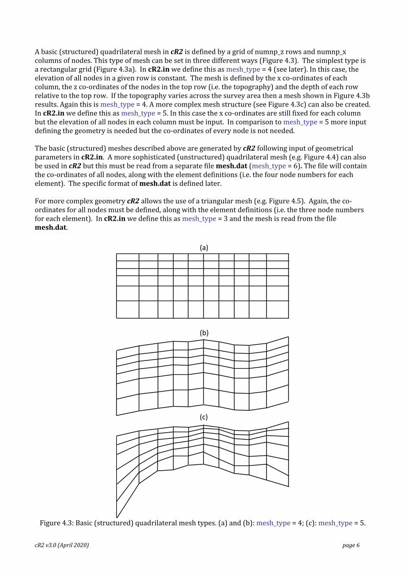
The mesh should clearly cover the survey area laterally and the expected depth of investigation, however, given that injected current will transfer further laterally and vertically, the mesh should extend sufficiently in order to account for this (mimicking infinite boundaries). There is no need to retain a fine discretisation in these ‘infinite’ boundary regions: it is good practice to let the elements gradually increase in size laterally and vertically outside the region of investigation. Figure 4.2 illustrates the zoning of discretisation. Note that this example is for a surface electrode array. For others, e.g. cross-borehole, similar concepts are applied.

Figure 4.2: Extending the finite element mesh to account for ‘infinite’ boundaries. DOI is the depth of investigation. Zone A is the region of interest; elements should be finely discretised especially near the

electrodes. Zone B has the same discretisation as A and is included to ensure good accuracy of the forward calculations; this zone typically extends two or three time the electrode spacing. Zone C

typically extends ~5L where L is the length of the longest current dipole. Discretisation should gradually get coarser in Zone C, moving away from the region of investigation.

1

2

3

71

77

1

2

6

55

60

7

Electrode array

~5L

~5L

DOI

B

A

C


A basic (structured) quadrilateral mesh in cR2 is defined by a grid of numnp_z rows and numnp_x columns of nodes. This type of mesh can be set in three different ways (Figure 4.3). The simplest type is a rectangular grid (Figure 4.3a). In cR2.in we define this as mesh_type = 4 (see later). In this case, the elevation of all nodes in a given row is constant. The mesh is defined by the x co-ordinates of each column, the z co-ordinates of the nodes in the top row (i.e. the topography) and the depth of each row relative to the top row. If the topography varies across the survey area then a mesh shown in Figure 4.3b results. Again this is mesh_type = 4. A more complex mesh structure (see Figure 4.3c) can also be created. In cR2.in we define this as mesh_type = 5. In this case the x co-ordinates are still fixed for each column but the elevation of all nodes in each column must be input. In comparison to mesh_type = 5 more input defining the geometry is needed but the co-ordinates of every node is not needed. The basic (structured) meshes described above are generated by cR2following input of geometrical parameters in cR2.in. A more sophisticated (unstructured) quadrilateral mesh (e.g. Figure 4.4) can also be used in cR2but this must be read from a separate file mesh.dat (mesh_type = 6).The file will contain the co-ordinates of all nodes, along with the element definitions (i.e. the four node numbers for each element). The specific format of mesh.dat is defined later. For more complex geometry cR2allows the use of a triangular mesh (e.g. Figure 4.5). Again, the co-ordinates for all nodes must be defined, along with the element definitions (i.e. the three node numbers for each element). In cR2.in we define this as mesh_type = 3 and the mesh is read from the file mesh.dat.

Figure 4.3: Basic (structured) quadrilateral mesh types. (a) and (b): mesh_type = 4; (c): mesh_type = 5.

(a)

(b)

(c)


Figure 4.4: Unstructured quadrilateral mesh example (mesh_type = 6).

Figure 4.5: Triangular mesh example (mesh_type = 3).

If full flexibility in mapping the geometry of the problem is required then a triangular mesh is preferred. In some instances the use of a pre-defined quadrilateral mesh (mesh_type = 6) may be effective. It doesn’t need to be unstructured. Figure 4.6 shows an example where rectangular geometry is used but since the mesh cannot be defined as one set of rows and columns, the mesh must be predefined and read from mesh.dat.

Figure 4.6: Structured quadrilateral mesh example (mesh_type = 6). Triangular meshes not only allow full flexibility in defining geometry but also result in more computationally efficient meshes since the extremities of the mesh can be made to have coarser discretisation (see Figure 4.7). If you are working with a triangular mesh then you must create the mesh and store details of the geometry of the mesh in a file mesh.dat. There are a number of good meshing tools available. Gmsh (see http://www. gmsh.info) is a powerful finite element mesh generator with a large user base with video tutorials available online. Alternatively, software for general finite element analysis (e.g. COMSOL) contain mesh generators, as do software for specific applications (e.g. groundwater code environments like GMS).


A key constraint of the structured meshes (mesh_type = 4 or 5) is that defining the geometry of parameter cells in an inverse solution is constrained (see section 5). If the mesh is prepared in mesh.dat (mesh_type = 3 or 6) the user has full control of parameter discretisation and zoning (see later). GmshmeshutilitycodesforcR2 The cR2 download package contains some simple codes for working with Gmsh. These are located in theMesh_utilities/Binley folder. GenGmshGeo2D creates a geometry file for Gmsh. This can then be loaded in Gmsh and a 2D mesh easily created. The mesh in Gmsh is saved as a file GenGmshGeo2D.msh which can be transformed to the mesh.dat format for cR2 using the partner code GmshMsh2R2. The code Check_R2_Tmesh can be run to check the mesh.dat file that is created. One thing that this code checks is the node numbering of the elements in the mesh. All finite elements should have node numbers in a counter-clockwise direction. Check_R2_Tmesh will check this and correct any such errors.

Figure 4.7: Example triangular mesh with variable discretisation.

Niels Claes (University of Wyoming) has provided a Matlab script (see folder Mesh_utilities/Claes) that will create a mesh file using Gmsh. Jimmy Boyd (British Geological Survey/ Lancaster University) has written a python script to covert Gmsh msh files tomesh.dat format for R2(orcR2). See Mesh_utilities/Boyd Again, note that these scripts have been produced with specific versions of Gmsh and may not be compatible with more recent versions. Also note that the author has not tested any of these third party scripts. Additionally, the graphical software ResIPy (https://pypi.org/project/resipy/) allows mesh generation within its interface of quadrilateral and triangular mesh.


5. Parameterisation For a forward model calculation the resistivity for each element must be defined. For an inverse solution the starting resistivity model must be defined. This is normally a uniform model. In inverse mode the discretisation of parameters must be set. The simplest way to do this is to set each finite element as a parameter. In some cases a more complex parameterisation is required. In a quadrilateral mesh we can define ‘patch’ sizes for parameters. A patch is a group of elements, which is illustrated in Figure 5.1. The advantage of such patching of elements is the reduced computational time, since the number of parameters is reduced. In some instances we may wish to fix the resistivity in part of the mesh, i.e. the parameters may only cover a subset of the finite element mesh (see, for example, Figure 5.2). cR2 allows this type of parameterisation by stating where the patching starts and ends in both x and y direction. Greater control of parameterisation is allowed for user-created triangular or quadrilateral mesh (e.g. Figure 5.3) by defining a parameter number for each element in mesh.dat. Note that if a parameter number 0 is assigned for an element then the inverse solution fixes the resistivity of this element to the starting value.

Figure 5.1: Defining parameter boundaries. The grey lines show the finite element mesh, the black lines show the parameter zones. (a) Each element is a parameter. (b) Each parameter is a 2 x 2 patch of

elements. (c) Each parameter is a 3 x 1 patch of elements.

(a)

(b)

(c)


Figure 5.2: Parameterisation of a subset of the finite element mesh. The grey lines show the finite element mesh, the black lines show the parameter zones.

Figure 5.3: Parameterisation of an unstructured mesh defined in mesh.dat. The grey lines show the finite

element mesh, the black lines show the parameter boundaries. Further control of parameterisation is achieved through ‘zoning’ of parameters (e.g. Figure 5.4). In cR2 a zone is defined as a congruent collection of parameters. Smoothing (in the inverse solution) does not occur across zones. This can be useful if aprioriinformation allows the user to define sharp contrasts (e.g. at a water table boundary).

Figure 5.4: Zoning of parameterisation. The grey shaded region is a different zone to the rest of the mesh.

Again, full flexibility is possible with an unstructured mesh (see Figure 5.5). For each element the parameter and zone is defined in the mesh.dat file.


Figure 5.5: Zoning of parameterisation in an unstructured triangular mesh. The three colours represent different parameter zones.

In summary, when a mesh is defined in mesh.dat, each element is assigned (i) a parameter number (which is zero if it should remain fixed throughout the inversion); (ii) a zone number. For most cases the parameter number of each element is the element number and the zone is 1.


6. Inputandoutputfiles

The input and output files used by cR2are shown schematically below, and described in detail later.

cR2requires at least two input files: cR2.inand protocol.dat. If a user-defined triangular or quadrilateral mesh is used then an additional input file – mesh.dat – is required. cR2.in contains information on the geometry of the problem to be solved. protocol.dat contains the measurement cR2 will output a number of files:


o cR2.out which will contain main log of execution. o electrodes.dat contains the coordinates of the electrodes.

If the problem to be run is a forward model then cR2 will output:

o cR2_forward.dat which will contain the forward model for the electrode configuration in protocol.dat The format of cR2_forward.dat is the same as protocol.dat:the first column is a measurement number, the next 4 columns contain the quadrupole electrode numbers, column 6 contains the calculated magnitudes, column 7 contains the phase angles in mrad, and column 8 contains the calculated apparent resistivities.

o forward_model.dat which will contain the resistivity distribution for your forward model (i.e.

what you specified in the input for cR2). Note that the format of these will be the same as described below for inverse mode.

o forward_model.vtk as above but vtk format (allowing plotting in ParaView, for example).

If the problem to be run is an inverse model then cR2 will output:

o f001_res.dat which will contain the resistivity result of the inverse solution.f001_res.dat will contain seven columns: x, z, resistivity magnitude, phase angle (in mrad), log10(resistivity magnitude), log10(real conductivity, in S/m), log10(imaginary conductivity, in S/m), where x,z are coordinates at centroid of each element and the other properties are for the that element. The format is setup to work directly with Surfer.

o f001_err.dat will contain nine columns. The first four columns contain the electrode numbers. In

the fifth column is the normalised data misfit, the next column contains the observed data recorded as an apparent resistivity, the next column contains the equivalent apparent resistivities for the computed model, the next column is the observed phase angles, the next column is the computed phase angles, the next column shows the original data weight (i.e. data standard deviation in same units as data), the next column is the final data weight, the last columns shows a "1" if any weights have been changed during the inversion, otherwise a "0" will appear.

o f001_res.vtk will contain resistivity magnitude, log10 resistivity magnitude, phase angle (in

mrad), log10 (real conductivity, in S/m), log10 (imaginary conductivity, in S/m), log10 (sensitivity) all in vtk format (allowing plotting in ParaView, for example). Here, sensitivity is defined as the diagonal of the matrix [JT WT W J] which gives an idea of the mesh sensitivity coverage (see Binley and Kemna, 2005).

o If you have more than one dataset in protocol.dat (see later) then the files f001_res.dat,

f002_res.dat,f003_res.dat, etc will be created. Similarly a set of _err.datfiles will be output. In additioncR2 will output:

o electrodes.dat, which contains the co-ordinates of the electrodes. The values are in three columns: x,z,y (where y is a dummy value – set to 0.0).

o electrodes.vtk contains the co-ordinates of the electrodes in vtk format. The values are in three

columns: x,z,y (the latter being set to zero). Use this file if you are working with Paraview to look at the resistivity images. Once you have opened the electrodes.vtk file in Paraview you select “apply” then you select the “Glyph” icon; this allows you to plot the electrodes as small spheres (or other objects).


NOTE:If cR2 fails to converge in inverse mode, all output files except the sensitivity map/resolution matrix will still be output in order to allow the user to assess the source of the problem (the fXXX.err file is useful for this) but the user should check the cR2.out file to ensure convergence is achieved before using any computed resistivity models. Somecommentsonco‐ordinatesignconventionWhen a quadrilateral mesh is created the user specifies the horizontal and vertical co-ordinates of the rows and columns forming the mesh. The convention here (see line 9 in cR2.in) is for the vertical co-ordinates to be specified as depth (not elevation). When these are output in a .dat file (e.g. forward_model.dat, for a forward model, or f001.dat, for an inversion) then the vertical co-ordinate sign is changed. This is so that programs like Surfer will show the section properly. The same switching of sign is changed in the vtk output (e.g. forward_model.vtk and f001.vtk). The electrode co-ordinates (output in electrodes.dat and electrodes.vtk) will also have a switched sign for the vertical co-ordinates. Triangular meshes should be created with the vertical co-ordinate representing elevation, not depth. And so when a triangular mesh is used, the sign change is not made in any of the output files listed above.


7. DetailsofcR2.in Line1: (Char*80) header

where header is a title of up to 80 characters Line 2: (2 Int, Real, 2 Int) job_type, mesh_type, flux_type

where job_type is 0 for forward solution only or 1 for inverse solution; mesh_type is 3 for triangular mesh or 4 for a regular quadrilateral mesh, 5 for a more generalised quadrilateral mesh or 6 for a general quadrilateral mesh (see section 5); flux_type is 2.0 for 2D current flow (i.e. line electrodes, which are infinitely long orthogonal to the section) or 3.0 (usual mode) for fully 3D current flow (i.e. point electrodes).

If mesh_type is 3 or 6 then the file mesh.dat must be supplied which contains the mesh details including node coordinates and element indices (see details later). If (mesh_type = 4) then a regular quadrilateral mesh is to be used and the following are read:

Line 3: (2 Int) numnp_x, numnp_z

where numnp_x is number of nodes in the x direction (horizontal) and numnp_z is the number of nodes in the z (vertical) direction

Line 4: (numnp_x Real) xx

where xx is an array containing x coordinates of each of numnp_x node columns

Line 5: (numnp_x Real) topog

where topog is an array containing elevations of each of numnp_x node columns. If the topography is flat then set topog to zero for all values.

Line 6: (numnp_z Real) zz

where zz is an array containing the depths of each of numnp_z node rows relative to the topog array. Set zz(1) to zero and the other values to a positive number (i.e. zz represents depth, not topography).

Else if (mesh_type = 5) then a more generalised quadrilateral mesh is to be used and the following are read:

Line 7: (2 Int) numnp_x, numnp_z where numnp_x is number of nodes in the x direction (horizontal) and numnp_z is the number of nodes in the z (vertical) direction

Line 8: (numnp_x Real) xx

where xx is an array containing x co-ordinates of each of numnp_x node columns

Line 9: (numnp_z Real) zz

where zz is an array containing elevations (not depths) of each of numnp_z node rows for column 1 in the x direction. For each column of nodes zz(1) is the topography.


Repeat Line 9 for all numnnp_x columns. End if Note: It is wise to add a carriage returns to break up a long list of input values (in Line 4, 5, 6, 8 and 9, for example). Don’t write more than 20 numbers on each line as the compiler may not like it. If (mesh_type = 3) then read the following

Line 10: (Real) scale where scale is a scaling factor for the mesh co-ordinates. This is usually 1.0 but if a standardised mesh is used, say for a unit circle, then this scaling factor is useful to adjust the mesh for a specific problem. Set scale=1 if you do not wish to change the coordinates of the mesh defined in mesh.dat.

End if Line 11: (Int) num_regions where num_regions is number of resistivity regions that will be specified either as starting condition for inverse solution or actual model for forward solution. The term “region” has no significance in the inversion – it is just a means of inputting a non-uniform resistivity as a starting model for inversion or for forward calculation. If (num_regions = 0) then read the following

Line 12: (15*Char) file_name where file_name is the name of the file containing the resistivitities from a previous inversion (the _res.dat file that had been produced). Note that the file_name must be no more than 15 characters and there should be no spaces before the file name and no characters in the line after the file name.

Else

Line 13: (2 Int, Real) elem_1, elem_2, mag, phase where the resistivity expressed as a magnitude (mag) and phase angle (phase) (in mrad) will be assigned for all elements from elem_1 to elem_2 (inclusive). Note that for a quadrilateral mesh the elements are numbered down columns first (top to bottom) then along rows (left to right).

Repeat Line 13 for all num_regions End if NOTE:youmustassignallelementsastartingvalue.Thenumberofelementsinthemeshis(numnp_x‐1)x(numnp_y‐1)foraquadrilateralmesh.Alltheseelementsmustbeassignedaresistivity.Notealsothatifyouassignanelementavalue,itwilloverwriteanypreviousassignment. If (job_type = 1. i.e. an inverse solution) then read the following

If (mesh_type = 4 or 5) then read the following

Line 14: (2 Int) patch_size_x, patch_size_z


where patch_size_x and patch_size_z are the parameter block sizes in the x and z direction, respectively. We differentiate between parameter size and element size to allow faster computation. The larger the patch size the few parameters and the faster the inversion, however, if we increase it too much we will reduce the flexibility to create variation of resistivity. If computational time is not a problem then use a patch size of 1 for x and z. Note that the number of elements in the x direction must be perfectly divisible by patch_size_x and the number of elements in the z direction must be perfectly divisible by patch_size_z otherwise set them both to zero. See examples in Figure 5.1. For Figure 5.1a patch_size_x =1 and patch_size_z = 1. For Figure 5.1b patch_size_x =2 and patch_size_z = 2. For Figure 5.1c patch_size_x =1 and patch_size_z = 3.

If (patch_size_x = 0) and (patch_size_z = 0) then read the following

Line 15: (2 Int) num_param_x, num_param_z where num_param_x and num_param_z are the number of parameter blocks in the x and z directions Line 16: (1+num_param_x Int) npxstart, npx(i), i=1,num_param_x where npxstart is the column number in the mesh where the parameters start; npx specifies the number of elements in each parameter block in the x direction Line 17: (1+num_param_z Int) npzstart, npz(i), i=1,num_param_z where npzstart is the row number in the mesh where the parameters start; npz specifies the number of elements in each parameter block in the z direction See example in Figure 5.2 (copied below). For this example we would set num_param_x = 12 and num_param_z = 9. Then we would set Line 17 as 3, 2,1,1,1,1,1,1,1,1,1,1,2 and Line 17 as 1, 1,1,1,1,1,1,1,1,2.

End if End if

NOTE:thefollowinglineinputisdifferenttov1.9andolderversionsofcR2

Line 18: (Int, Real) inverse_type, target_decrease where inverse_type is 0 for pseudo-Marquardt solution or 1 for regularised solution with linear filter (usual mode) or 4 for blocked linear regularised type (see also line 21). Note that the blocking defined here is only for a quadrilateral mesh – for blocking within a triangular mesh see the details for preparing mesh.dat later. target_decrease is a real number which allows the user to specify the relative reduction of misfit in each iteration. A value of 0.25 will mean that cR2 will


aim to drop the misfit by 25% (and no more) of the value at the start of the iteration. This allows a slower progression of the inversion, which can often result in a better convergence. If you set target_decrease to 0.0 then cR2 will try to achieve the maximum reduction in misfit in the iteration.

Line 19: (Real, 2 Int, Real) tolerance, max_iterations, error_mod, alpha_aniso where tolerance is desired misfit (usually 1.0); max_iterations is the maximum number of iterations; error_mod is 0 if you wish to preserve the data weights, or 2 if you wish the inversion to update the weights as the inversion progresses based on how good a fit each data point makes. The routine used is based on Morelli and LaBrecque (1996). Note that no weights will be increased. The smoothing factor used in the code (alpha) is searched for at each iteration. The search is done over a range of steps in alpha, the number of steps is 10. alpha_aniso is the anisotropy of the smoothing factor, set alpha_aniso > 1 for smoother horizontal models, alpha_aniso < 1 for smoother vertical models, or alpha_aniso=1 for normal (isotropic) regularisation. Line 20: (5 Real) min_error, a_wgt, b_wgt, rho_min, rho_max

where min_error is the minimum magnitude error (this is to ensure that very low errors are not assigned and is only used if a_wgt and b_wgt are both zero), a_wgt and b_wgt are error variance model parameters: a_wgt is the relative error of magnitudes; b_wgt is absolute error of phase values (in mrad); rho_min and rho_max are the minimum and maximum observed apparent resistivity magnitude to be used for inversion (use large extremes if you want all data to be used). NOTE that if your mesh contains topography, or the surface elevation is not zero, or the left, right and lower extent of the mesh does not represent infinite boundaries then the geometric factor computed in the code will be incorrect and thus any comparison of apparent resistivities against upper and lower limits will be invalid. For such a case you should set rho_min and rho_max to be very low and very high values, e.g. -10e10 and 10e10, respectively. Note also that you can select to include individual errors for each measurement in the data input file protocol.dat – to do this a_wgt and b_wgt should be set to 0.0. If a_wgt and b_wgt are set to zero then protocol.dat must contain errors for the data weights (see next section). It is advisable to estimate a_wgt and b_wgt from error checks in the field data (ideally from reciprocal measurements - not measures of repeatability). Typically for surface data a_wgt will be about 0.02 (equivalent to 2% error), b_wgt will be typically 2mrad for good data, but could be much higher. Line 21: (num_param_x Int) param_symbol If you have specified zoning of parameters (inverse_type = 4 in line 18) so that each zone is disconnected from other zones then for a quadrilateral mesh (see Figure 4.9) the zones are specified by producing a simple plan of the parameter mesh. You must input for each row of parameters an integer representing the parameters. This is repeated for each row. Make sure that you put a space between each integer. As an example consider the zoned mesh in Figure 4.9 (copied below) with 20 elements in the x direction and 12 elements in the z direction. In this example we wish to zone the region shaded. As each element is a parameter then the patch size in x and z is 1, so in total there are 20 parameters (x) by 12 parameters (z). If we want to set the boundary of the shaded region so that there is no smoothing to the unshaded region then we would input: 1 1 1 1 2 2 2 2 2 2 2 2 2 2 2 2 1 1 1 1 1 1 1 1 2 2 2 2 2 2 2 2 2 2 2 2 1 1 1 1 1 1 1 1 2 2 2 2 2 2 2 2 2 2 2 2 1 1 1 1 1 1 1 1 2 2 2 2 2 2 2 2 2 2 2 2 1 1 1 1 1 1 1 1 2 2 2 2 2 2 2 2 2 2 2 2 1 1 1 1 1 1 1 1 2 2 2 2 2 2 2 2 2 2 2 2 1 1 1 1


1 1 1 1 2 2 2 2 2 2 2 2 2 2 2 2 1 1 1 1 1 1 1 1 2 2 2 2 2 2 2 2 2 2 2 2 1 1 1 1 1 1 1 1 1 1 1 1 1 1 1 1 1 1 1 1 1 1 1 1 1 1 1 1 1 1 1 1 1 1 1 1 1 1 1 1 1 1 1 1 1 1 1 1 1 1 1 1 1 1 1 1 1 1 1 1 1 1 1 1 1 1 1 1 1 1 1 1 1 1 1 1 1 1 1 1 1 1 1 1 Note that we have used 1s and 2s to define the regions. We could have used any other integer.

If for the problem above we had a patch size of 2 in x and z then Line 21 would be: 1 1 2 2 2 2 2 2 1 1 1 1 2 2 2 2 2 2 1 1 1 1 2 2 2 2 2 2 1 1 1 1 2 2 2 2 2 2 1 1 1 1 1 1 1 1 1 1 1 1 1 1 1 1 1 1 1 1 1 1 If we had defined the problem to have a patch size in x of 4 and a patch size in z of 2 then Line 21 would be: 1 2 2 2 1 1 2 2 2 1 1 2 2 2 1 1 2 2 2 1 1 1 1 1 1 1 1 1 1 1 Repeat line 21 for all num_param_z End if

End if Line 22: (Integer) num_xz_poly where num_xz_poly is the number of x,z co-ordinates that define a polyline bounding the output volume. If num_xz_poly is set to zero then no bounding is done in the x-z plane. The co-ordinates of the bounding polyline follow in the next line. NOTE: the first and last pair of co-ordinates must be identical (to complete the polyline). So, for example, if you define a bounding square in x,z then you must have 5 co-ordinates on the polyline. The polyline must be defined as a series of co-ordinates in sequence, although the order can be clockwise or anti-clockwise (see examples later). NOTE: cR2 stores the vertical co-ordinates for nodes in a structured quadrilateral mesh with a convention positive upwards. For example, if the ground surface has an elevation of 0m and you wish to output to a depth of 8m then z=-8m must be used for the lower boundary of the polygon. Similarly, if the ground surface elevation is 100m and you wish to output to a depth of 8m then z=-92m must be used for the lower boundary of the polygon. If a


user-defined triangular or quadrilateral mesh is used (i.e. supplied in mesh.dat) then the co-ordinates specified in the mesh file are used and the above comments about sign convention do not apply. Line 23: (2 Real) x_poly(1), z_poly(2) where x_poly(1), z_poly(1) are the co-ordinates of the first point on the polyline. Repeat line 23 for all num_xz_poly co-ordinates. Line 24: (Int) num_electrodes where num_electrodes is number of electrodes If (mesh_type = 3 ) then

Line 25: (2 Int) j, node where j is the electrode number and node is the node number in the finite element mesh

Else

Line 26: (3 Int) j, column, row where j is the electrode number, column is the column index for the node the finite element mesh and row is the row index for the node in the finite element mesh. The column value must be in the range 1 to numnp_x and the row value must be in the range 1 to numnp_z. Both values must be integer values.

End If Repeat Line 25/26 for all num_electrodes END OF INPUT FOR cR2.in


8. Detailsofprotocol.dat protocol.dat contains measurement schedule (and data for inverse if selected) Line 1: (Int) num_ind_meas where num_ind_meas is number of measurements to follow in file If (job_type = 1) then

If (a_wgt = 0 AND b_wgt = 0) then

Line 2: (5 Int, 4 Real) j, elec(1,k), elec(2,k), elec(3,k), elec(4,k), mag, phase, mag_error, phase_error where j is not used (but usually is used as a measurement number in the file); elec(1,k) is the electrode number for the P+ electrode; elec(2,k) is the electrode number for the P- electrode; elec(3,k) is the electrode number for the C+ electrode; elec(4,k) is the electrode number for the C- electrode; measured resistivity has magnitude mag (in ) and phase angle phase (in mrad), mag_error is absolute error in magnitude (in ), phase_error is the phase error (in mrad).

Else

Line 2: (5 Int, 2 Real) j, elec(1,k), elec(2,k),elec(3,k),elec(4,k), mag, phase where j is not used (but usually is used as a measurement number in the file); elec(1,k) is the electrode number for the P+ electrode; elec(2,k) is the electrode number for the P- electrode; elec(3,k) is the electrode number for the C+ electrode; elec(4,k) is the electrode number for the C- electrode; measured resistivity has magnitude mag (in ) and phase angle phase (in mrad).

End if

Repeat Line 2 for all num_ind_meas Else (for forward solution only)

Line 3: (5 Int) j, elec(1,k), elec(2,k), elec(3,k), elec(4,k) where j is not used (but usually is used as a measurement number in the file); elec(1,k) is the electrode number for the P+ electrode; elec(2,k) is the electrode number for the P- electrode; elec(3,k) is the electrode number for the C+ electrode; elec(4,k) is the electrode number for the C- electrode. Repeat Line 3 for all num_ind_meas

End if You can add as many datasets to the file protocol.dat. Just concatenate the datasets into one file. cR2will continue to read and process data using the settings defined in cR2.in END OF INPUT FOR protocol.dat


9. Detailsofmesh.dat It is useful if your mesh generator permits ‘materials’ to be defined, allowing some zoning of the mesh (to permit blocking at interfaces). Also, you may find it beneficial (for computational efficiency) to create a coarse mesh to define the parameters and then refine this mesh (splitting a triangle element into more elements) to have more elements for the forward solution. The simplest mesh consists of an equal number of parameters and elements and one zone. More complex arrangements allow for grouping of elements into parameters and multiple zones. Regularisation is not applied at the interface of zones. NOTE:Line 1 changed from version 3.3 Line 1: (2 Int) numel, numnp, ndirichlet Where numel is the number of triangle elements, numnp is the number of nodes and ndirichlet is the node number of a specified dirichlet node, which should be a node far away from all electrode nodes. If ndirichlet is set to zero then the code will compute the node that is furthest away. However, for some geometries (e.g. a circular region) the node that is the furthest away based on average distance may be close to one of the nodes. For such problems it is advisable to set the node in the centre of the mesh as the dirichlet node to avoid biasing of the computed potential field. Line 2: (6 Int) n, index(1,n), index(2,n), index(3,n), param(n), zone(n) Where n is the element number; index(1,n), index(2,n) and index(3,n) are the node numbers of the element, numbered in a counter-clockwise direction (cR2 will check if this is correct for a triangular or quadrilateral mesh that is read from mesh.dat); param(n) is the parameter number of the element (to make every element a parameter then make this value equal to the element number); zone(n) is the zone number for element n. To have one zone make zone(n) equal to 1 for all elements. Zones must be connected elements. Parameters cannot occupy more than one zone. NOTE also, to make an parameter fixed to the starting resistivity, set param(n) to zero but note that if this is done all elements with param(n) = 0 must be at the end of the block of elements (see Surface 8 example below). This will involve reordering elements and care must be taken to ensure that any associated files with the element mapping (e.g. a start resistivity file, if used) but follow the same new element numbering. Repeat line 2 for all numel elements. Line 3: (Int, 2 Real) n, x(n), z(n) Where n is the node number; x(n), z(n) are the coordinates of node n. Repeat line 3 for all numnp nodes. END OF INPUT FORmesh.dat


10. ExamplesThe folder “Examples” contains a number of worked examples of cR2 to illustrate how to setup input files and work with model output. Surfaceelectrodearray1–gettingstartedThe subfolder “Examples/Surface_1” contains an example synthetic model of a surface electrode array using a dipole-dipole measurement scheme. The example is a modification of the one in Binley and Kemna (2005). For this problem 25 electrodes are positioned at 2m spacing on a flat surface of a half space. The electrodes are numbered 1 to 25 from left to right. A forward model is setup to determine the measured transfer resistances for a dipole-dipole scheme with 117 measurements. The resistivity model is shown in Figure 10.1. A small target with resistivity 10 m, -10mrad lies within a 100 m. -10mrad half space: positioned vertically between depths 1m and 4m and horizontally between 14m and 16m.

Figure 10.1: Definition of synthetic model for surface array 1 problem

The subfolder “Examples/Surface_1/Forward” contains the protocol.dat file for the forward problem. Also contained in the folder is the file cR2.in which defines the geometry and resistivity model. Since the model is a half space the finite element mesh must extend significantly away from the region of investigation (horizontally and vertically downwards). The mesh developed consists of 225 node columns and 49 node rows (i.e. 11,025 nodes, 10,752 elements). The file cR2.in shows how the mesh is designed to get progressively coarser away from the region of study. Note that the co-ordinates of the mesh have been set so that electrode 1 is at (0,0) for this problem. In the mesh electrode 1 is located at node column 17 (i.e. there are 16 elements to the left of the electrode array to represent an infinite boundary condition to the left. For this example 8 elements are placed between electrodes and so node 2 is at node column 25, node 3 is at column 33, etc. Since the electrodes are located on the ground surface the row node for all electrodes is 1. All the electrode positions are assigned in cR2.in. The file also assigns the resistivity for all elements. For this problem it is done by defining the resistivity of 9 congruent blocks of elements. First all elements in the mesh are set to 100 m, -10mrad and then 8 columns of vertically adjacent elements are defined to set the 10 m, -100mrad anomaly (remember that the elements are numbered vertically then horizontally). When cR2 is run the output files are:

cR2.out, which contains the main log of execution electrodes.dat, which contains the electrode co-ordinates electrodes.vtk, which contains the electrode co-ordinates in vtk format cR2_forward.dat, which contains the forward model, i.e. the 117 impedances. Note that the apparent resistivity for each of the 117 measurements is also stored. forward_model.dat, which contains the co-ordinates of the centroid of each finite element in the mesh, the resistivity magnitude and phase angle of each finite element along with the logarithm (to base 10) of the resistivity and the real and imaginary conductivity. This file is useful for checking if the resistivities were defined correctly in cR2.inforward_model.vtk, which contains the forward model in vtk format (see Figure 10.2).

0 5 10 15 20 25 30 35 40 45-8

-4

0

Distance (m)

Depth (m) Electrode10 m

-100 mrad100 m-10 mrad


Figure 10.2: Paraview plot of forward_model.vtk

The subfolder “Surface_1/Inverse” contains files for running the inversion of the transfer resistances determined above. For this a uniform starting resistivity of 100 m, 0mrad is defined in the file cR2.in. The ‘data’ to be inverted are stored in file protocol.dat: here the values are simply the impedances (magnitude and phase angle) that appeared in the cR2_forward.dat file described earlier. For the inverse problem we have used a patch_size of 4 in both x and z directions, i.e. each inverse parameter is a 2 by 2 block of finite elements. When cR2 is run in this case the output files are:

cR2.out, which contains the main log of execution; electrodes.dat, which contains the electrode co-ordinates; electrodes.vtk, which contains the electrode co-ordinates in vtk format f001_res.dat, which contains the computed resistivity magnitude and phase angle, log10 resistivity magnitude, real and imaginary conductivity for each finite element in the output region defined in cR2.in; f001_res.vtk, which, in vtk format, contains the values in f001_res.dat and also the sensitivity map; f001_err.dat, which contains the misfit for each of the 117 measurements.

Figure 10.3 shows the results of the inversion (compare with Fig 5.8 of Binley and Kemna(2005)). This is an image map of the results in f001_res.vtk. The file f001_res.dat could also have been used, e.g. with Surfer. Note that only the region within the electrode array and to a depth of 8m has been plotted.


In Figure 10.4 the sensitivity map is also shown. The values are computed with the equation 5.20 of Binley and Kemna (2005). High values indicate areas of high measurement sensitivity.

Figure 10.3: Inverse model for surface array 1 problem with dp-dp array

Figure 10.4: Sensitivity map for inverse model for surface array 1 problem with dp-dp array

Surfaceelectrodearray2–addingtopographyThe subfolder “Examples/Surface_2” contains an example similar to the previous case but with varying surface topography. Here the ground surface slopes from 0m at electrode 1 to 1m in the centre of the electrode array and then drops back to 0m at electrode 25 (see Figure 10.5). The file cR2.in is now


different for the forward and inverse model runs through the addition of topography data. Figure 10.6 shows the inverse solution for this case.

Figure 10.5: Definition of synthetic model for surface array 2 problem

Figure 10.6: Inverse model for surface array 2 problem


Surfaceelectrodearray3–triangularmeshingThe folder Examples/Surface_3/ contains input files for running a forward and inverse problems for the dipole-dipole survey (from Surface electrode array 1) using a triangular mesh. The mesh is defined in mesh.dat. It contains 4,204 elements and 2,160 nodes. The region modelled extends approximately 200m to the left and right of the electrode array, and approximately 200m beyond the zone of investigation. The folder Examples/Surface_3/Forward contains the input files for a forward model. In this mesh the first 40 elements represent the 10m, -100mrad anomaly: in cR2.in the two regions are defined. Figure 10.7 shows a plot of the forward model definition using ParaView. Note that the region extracted for plotting is based on the position of the centroid of elements and consequently a ‘jagged’ boundary often exists for triangular mesh output.

Figure 10.7: Definition of forward model using a triangular mesh The folder Examples/Surface_3/Inverse_1 contains the input files for an inversion of the data using a triangular mesh. Figure 10.8 shows the result, plotted in ParaView. Figure 10.9 shows the sensitivity map for this problem.


Figure 10.8: Inversion of dipole-dipole data.

Figure 10.9: Sensitivity map for triangular mesh problemThe folder Examples/Surface_3/Inverse_2 contains the input files for an inversion of the same data using anisotropic regularisation to minimise lateral smoothing (see Figure 10.10).

Figure 10.10: Inversion of dipole-dipole data with enhanced vertical smoothing.


The folder Examples/Surface_3/Inverse_3 contains the input files for an inversion of the same data as above but in this example the inverse region is blocked into two zones: one representing the low resistivity magnitude/high phase angle zone in Figure 10.7 and the other representing the remainder of the mesh. In this case the 40 elements that occupy the area where the low resistivity feature exists are given a different zone to the other elements in the mesh (see input for mesh.dat). These 40 elements are 4165 to 4204 in mesh.dat: a zone number of 2 is assigned to them (zone = 1 is assigned to the other elements). Figure 10.11 shows the resulting inversion. The inversion has been forced to honour the known boundaries and as a result the solution is near perfect. There is subtle variation in the zones, however – see lower image in Figure 10.11.

Figure 10.11: Inversion of dipole-dipole data with region blocking. The lower figure is included to show

that variation does exist within the zones. The folder Examples/Surface_3/Inverse_4 contains input files to illustrate the effect of fixing resistivity using a triangular mesh. In this example we set the resistivity of some elements to a fixed value. To do this we set their parameter number to zero in mesh.dat. Note that to do this we have to move this block of elements in mesh.dat to the end of the list of elements.In this example we set the 40 elements in the ‘anomaly’ area to be fixed to whatever value is assigned as the starting model (in cR2.in) (in this case 20 m, -20mrad). All other elements can change in the inversion. The inversion is show in Figure 10.12.


Note that the true target is 10 m and -100 mrad and so by forcing the region to be 20 m and -20mrad the adjacent elements are affected as the inversion compensates for the difference.

Figure 10.12: Inversion of dipole-dipole data with 40 elements (where the ‘target’ is located) set to 20 m, -20mrad (the true value is 10 m, -100mrad and so some smearing around the ‘target zone’ exists). Surfaceelectrodearray4–quadrilateralmeshinmesh.datThe folder Examples/Surface_4/ contains input files for running a forward and inverse problem when a quadrilateral mesh is read from mesh.dat (i.e. mesh_type = 6). The example used here is the same setup as Surface electrode array 1 using a dipole-dipole configuration, but rather than defining a mesh in cR2.in, it is read from the file mesh.dat. Figure 10.13 shows the inverse model. Clearly for this problem the use of a separate mesh file is unnecessary, but it allows the user to understand the way in which a pre-defined quadrilateral mesh can be used.


Figure 10.13: Inversion of dipole-dipole surface electrode data using quadrilateral mesh read from

mesh.dat Surfaceelectrodearray5–fieldexampleThe folder Examples/Surface_5/ contains input files for a field survey from a UK site. The purpose of the survey was to identify the depth of a sandstone aquifer and the nature of the superficial (glacially deposited) sediments above it, with a view to assessing the vulnerability of the sandstone to surface sourced contamination. The survey was carried out in time domain IP mode with an Iris Syscal Pro using 48 electrodes at 2m spacing. Measured transfer resistances and chargeabilities were converted to equivalent magnitudes and phase angles. Figure 10.14 shows the resulting inversion. Figure 10.13 also shows the sensitivity map for the inversion. The sandstone boundary is approximately 10m deep (confirmed by drilling). The clay rich sediments above are revealed by low resistivity magnitude and a low phase angle. For more information see Mejus (2014). In this example the data errors are set for each measurement in protocol.dat.


Figure 10.14: Inversion of field data.

FinalnoteonexamplesThe examples included should give the user a good start in setting up files for their own datasets. Again, it is strongly recommended that the user becomes familiar with sister code R2 before working with cR2. The examples provided with R2 show how cross-borehole surveys can be inverted – exactly the same approach can be followed with cR2. When working with inversion of field data if problems occur then it is recommended that the user runs a forward model with the measurement set to check that computed values from this make sense. Many problems I hear about could have been avoided by running such tests. Finally, as R2 has a 3D equivalent R3t, cR2also has a 3D version cR3t. Copies are available from the author


11. Additionalcodesandscripts

The cR2 package contains a number of codes and scripts that may help the user in creating input files and visualising output from cR2. If you are interested in other scripts then download the sister code R2 – a number of additional third party scripts and codes are included. Meshing Folder Mesh_Utilities/Binley GenGmshGeo2D.exeCreates a Gmsh geo (geometry file) which may be used for creating a triangular mesh. Note that the geo file can be edited before meshing, e.g. to add topography. The geo file created is GenGmshGeo2D.geo GmshMsh2R2.exeReads the GenGmshGeo2D.geocreated (and, perhaps, edited) in Gmsh, which can be meshed, creating a msh (mesh file) mesh.dat.Note that the first line will contain the number of elements, which is needed in cR2.in for defining the resistivity (starting model or forward model definition). Check_R2_Tmesh Run to check the mesh.dat file that is created and fix errors, in particular node numbering of the elements in the mesh. Folder Mesh_Utilities/Boydgmsh2R2mshThis python code and executable (written by Jimmy Boyd (British Geological Survey/Lancaster University) with convert a Gmsh msh file to an R2 (or cR2) mesh.dat file. Folder Mesh_Utilities/Claes create_meshA Matlab script written by Niels Claes (Wyoming University) will create an R2 (orcR2)mesh.dat file for a triangular mesh.

ResIPy (Python interface) Guillaume Blanchy (Lancaster), Sina Saneiyan (Rutgers) , Jimmy Boyd (BGS/Lancaster), Paul McLachlan (Lancaster/BGS) have developed an open source python GUI for R2 and sister codes (including cR2). See Blanchy et al.(2020). See also https://gitlab.com/hkex/pyr2 which also includes links for standalone executables. More information is also available at https://www.researchgate.net/project/ResIPy-GUI-for-R2-family-codes


12. GettingstartedwithParaViewThe vtk files created by cR2 have been structured to work in ParaView - an open source visualisation application that can be downloaded from https://www.paraview.org/ Users are advised to study online tutorials on ParaView. Here are a few simple tips to help the user get going. The fXXX_res.vtkfile contains the inverted resistivity magnitude, phase angle, log10 transformed resistivity magnitude, log10 real conductivity, log10 imaginary conductivity and a sensitivity map. The file also contains the finite element mesh structure. Open a fXXX_res.vtk file in ParaView, click Apply under Properties and you will get a map of the resistivity. Under Coloring in Properties you can select one of other variables stored, e.g. log10resistivity. The default Representation of the image is Surface. Change to Surface with edges to see the finite element mesh and the resistivity image. Axis labels and the colour legend are easily changed to suit the user. To get an interpolated image (rather than one that shows element by element) then highlight the vtk file in the Pipeline Browser and select the Cell Data to Point Data Filter. Then select Apply in Properties. If you want to show an image with thresholded values based on the sensitivity map then select the Clip icon and then Clip Type as Scalar under Properties and select Sensitivity(log10) as Scalars. Select a mid-range value in the slider bar for Value. Under Coloring select Magnitude (ohm.m). You should now see the thresholded region as a solid colour. If you wish to retain the full image with the thresholded area opaque then select the f001_res.vtk image and then select Opacity under Styling as a value less than 1. To show the electrodes, open the electrodes.vtk file and click Apply under Properties. Now select Point Gaussian under the Representation under the Display options. The screenshot below shows an sample from the Surface 1 example.


13. CommonUserErrorsBelow is a list of some common user errors that I have encountered. This may be useful for new users. A common mistake is for a new user to go straight into trying to run an inverse solution without getting a good feeling for the model that is being used. New (and old) users working on new problems should first try run a forward model for a uniform resistivity. This will help sort out any problems with the definition of the mesh, etc. It will also be useful in understanding the quality of the forward model and help judge this against the quality of the data. If you can, run the code from the command line. You will need to run CMD in Windows, then move to the correct folder and then type cR2.Doing it like this help see any errors if the program crashes unexpectedly because of incorrect input. In the example input files provided there are comments at the end of most lines in the form “<< comment” . Note that these are always at the end of a line. You cannot have these appearing on their own in a line. If you do then cR2will try read this comment when it is expecting numerical input and simply crash. The mesh is based on elements and nodes. In cR2.inLines 3 to 9 are based on nodes, whereas Line 13 is based on elements. It is important to understand the difference and not mix the two. On Line 18 in cR2.in, specifying a tolerance of 1.0 means that you are happy that you have estimated your errors correctly (Line 19). Don’t just use the a_wgt and b_wgt values in the example files – spend time to understand the likely errors in your measurements and model. Setting the minimum and maximum apparent resistivity (Line 19 of cR2.in) is only valid if you have a flat surface and an infinite half space problem, otherwise the geometric factors that cR2 will compute will be incorrect. For a quadrilateral mesh the electrode positions are defined by their column and row positions in the mesh (Line 25 of cR2.in). These are not the co-ordinates of the electrodes but their position in the mesh. In the definition of the input files, each line has been defined in terms of the type of numbers that are required. For example, (Real, 2 Int, 2 Real) means one real number, followed by two integers, followed by two reals. You can substitute integers for reals but not the other way round. So if the code is expecting an integer and your line entry has 1.3, for example, then the code will crash. Note that the data in protocol.dat should be provided in transfer resistances, NOT apparent resistivities. Also note that the polarity should be reflected in the phase angle (see section 3). It is very wise to check the polarity of your measurements – you can do this by computing the geometric factor for your measurement configuration (provided topographic and non-infinite boundaries are not significant). If you don’t know how to compute the geometric factors then you should run a forward model with cR2for a uniform half space and compare the computed polarities with those in your data. For a surface electrode array your data should be the same polarity as the model, otherwise the measurements will not be included in the inversion. For electrodes not on the surface the polarity can change as the resistivity structure changes in the inversion. Make sure you check that the solution has converged in inverse mode (see cR2.out). Just because a resistivity model has been computed it does not mean that convergence has been reached. If the solution has not converged then go through the fXXX.errfile and look at see if any particular measurements are problematic. Also check that you are confident with the a_wgt and b_wgt error settings you have applied (Line 19, cR2.in). A common mistake is to set these too low. A good estimate of a_wgt is important for the magnitude inversion and b_wgt is critical for the phase angle . Normally,


you should be able to get convergence in less than 5 iterations for the magnitude and typically only one iteration for the phase angle improvement. It is not wise to increase the maximum number of iterations to a large number. If you don’t get convergence in 10 iterations then there is definitely some problem with the data, the assumptions or the input files.


14. References Binley, A., 2015, Tools and Techniques: DC Electrical Methods, In: Treatise on Geophysics, 2nd Edition, G Schubert (Ed.), Elsevier., Vol. 11, 233-259, doi:10.1016/B978-0-444-53802-4.00192-5. (available from the author on request). Binley, A. and A. Kemna, 2005, Electrical Methods, In: Hydrogeophysics by Rubin and Hubbard (Eds.), 129-156, Springer Blanchy, G., S. Saneiyan, J. Boyd, P. McLachlan and A. Binley, 2020, ResIPy, an intuitive open source software for complex geoelectrical inversion/modeling in 2D space, Computer & Geosciences, 137, doi: 10.1016/j.cageo.2020.104423. Kemna, A., A. Binley and L. Slater, 2004, Cross-borehole IP imaging for engineering and environmental applications, Geophysics, 69(1), 97-105. Kemna, A., E. Räkers, and A. Binley, 1997, Application of complex resistivity tomography to field data from a kerosene-contaminated site: Environmental and Engineering Geophysics (EEGS) European Section, 151–154. Mejus, L., 2014, Using multiple geophysical techniques for improved assessment of aquifer vulnerability, PhD thesis, Lancaster University, UK. Mwakanyamale, K., L. Slater, A. Binley and D. Ntarlagiannis, 2012, Lithologic Imaging Using Induced Polarization: Lessons Learned from the Hanford 300 Area, Geophysics, 77, 397-409. IfyoumakeuseofcR2thenpleasecontacttheauthor([email protected])sothatyoucan

beaddedtoamailinglistforfutureupdates,fixes,etc.

Formoreinformation,includingexamplefilescontact:

Andrew Binley Lancaster Environment Centre

Lancaster University Lancaster LA1 4YQ, UK

Email: [email protected]

cR2 v3.0 readme - es.lancs.ac.uk

Documents

Transcript of cR2 v3.0 readme - es.lancs.ac.uk