CPU Scheduling

Section 2.4: Tanenbaum’s bookChapter 5: Silberschatz’s book

Kartik Gopalan

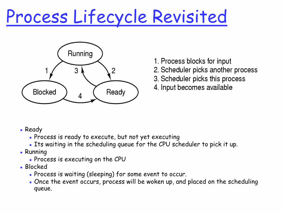
Process Lifecycle Revisited

● Ready● Process is ready to execute, but not yet executing● Its waiting in the scheduling queue for the CPU scheduler to pick it up.

● Running● Process is executing on the CPU

● Blocked● Process is waiting (sleeping) for some event to occur.● Once the event occurs, process will be woken up, and placed on the scheduling

queue.

CPU scheduler

● Selects the next process to run on the CPU from among the processes that are ready to execute

● CPU scheduling decision may take place when any process:1. Switches from running to waiting state2. Switches from running to ready state (pre-emptive scheduling)3. Switches from waiting to ready4. Terminates

3

CPUWho’s Next?

CPU SchedulerQueue of Ready Process

CS350/BU

Dispatcher

● Not the same as scheduler.

● Dispatcher gives control of the CPU to the process selected by the scheduler; this involves:o switching contexto switching to user modeo jumping to the proper location in the user program to

restart that program

● Dispatch latency● Time it takes for the dispatcher to stop one process and

start another running

CS350/BU

Linux CPU Scheduling Code● To browse, go to http://lxr.free-electrons.com

● To download, modify, and compile, go to● http://ftp.kernel.org/

● Scheduling code is located under● kernel/sched/core.c

● Three ways to invoke kernel code● System calls● Hardware interrups● Exceptions

● For x86, all entry points into the 4.2 kernel are located in assembly code in● arch/x86/entry/entry_32.S● OR arch/x86/entry/entry_64.S

CS350/BU

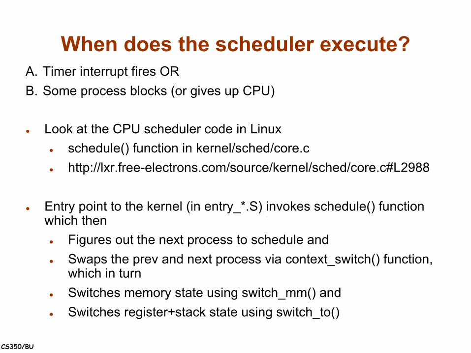
When does the scheduler execute?A. Timer interrupt fires OR B. Some process blocks (or gives up CPU)

● Look at the CPU scheduler code in Linux● schedule() function in kernel/sched/core.c● http://lxr.free-electrons.com/source/kernel/sched/core.c#L2988

● Entry point to the kernel (in entry_*.S) invokes schedule() function which then

● Figures out the next process to schedule and● Swaps the prev and next process via context_switch() function,

which in turn● Switches memory state using switch_mm() and ● Switches register+stack state using switch_to()

CS350/BU

Scheduling Criteria● CPU utilization – keep the CPU as

busy as possible● Throughput – Number of

processes that complete their execution per time unit

● Turnaround time – amount of time to execute a particular process, from submission to termination.

● Waiting time – amount of time a process has been waiting in the ready queue

● Response time – amount of time it takes from when a request was submitted until the first response is produced.

Optimization Criteria● Max CPU utilization

● Max throughput

● Min turnaround time

● Min waiting time

● Min response time

CS350/BU

Different systems have different scheduling goals

CS350/BU

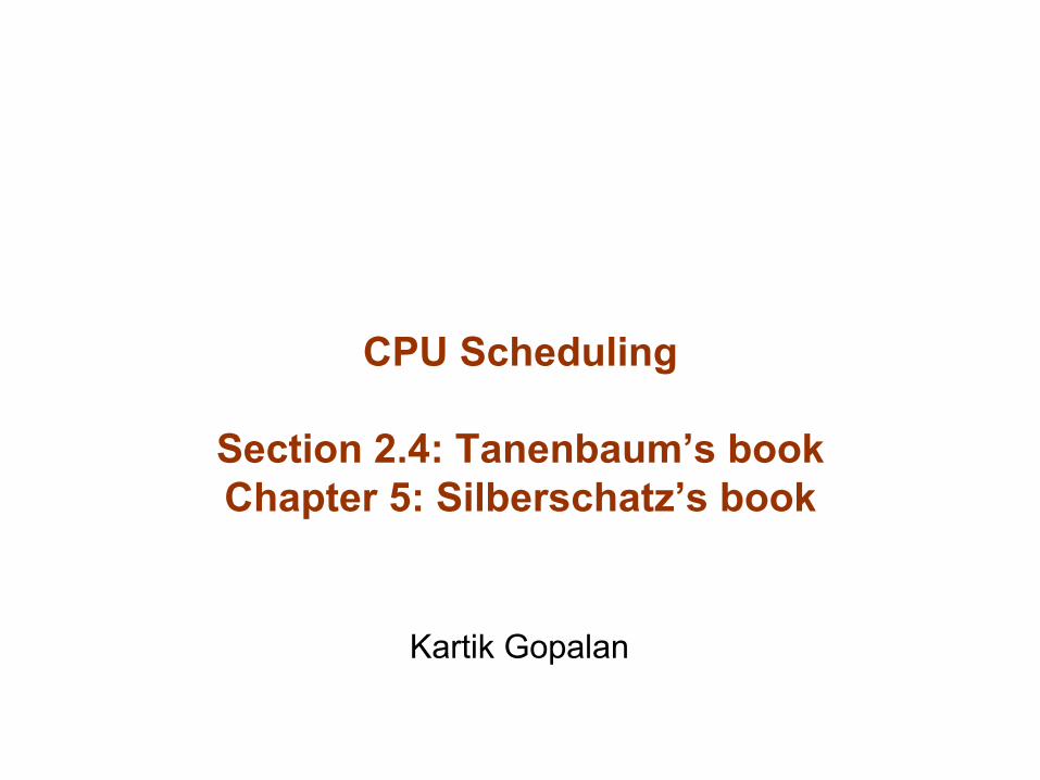
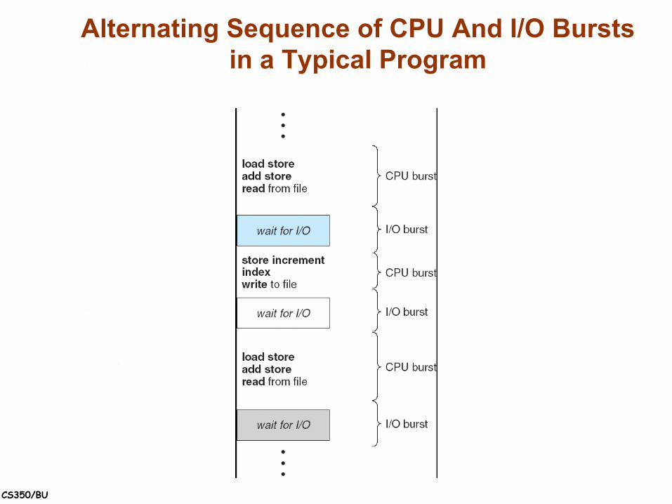
Alternating Sequence of CPU And I/O Bursts in a Typical Program

CS350/BU

Alternating Sequence of CPU And I/O Bursts (contd)

● A CPU-bound process

● An I/O-bound process

CS350/BU

First-Come, First-Served (FCFS) Scheduling

Process Burst TimeP1 24P2 3P3 3

Suppose that the processes arrive in the order: P1 , P2 , P3 The Gantt Chart for the schedule is:

● Waiting time for P1 = 0; P2 = 24; P3 = 27● Average waiting time: (0 + 24 + 27)/3 = 17

P1 P2 P3

24 27 300

CS350/BU

FCFS Scheduling (Cont.)

Suppose that the processes arrive in the orderP2 , P3 , P1

● The Gantt chart for the schedule is:

● Waiting time for P1 = 6; P2 = 0; P3 = 3● Average waiting time: (6 + 0 + 3)/3 = 3● Much better than previous case● Convoy effect : short process behind long process

P1P3P2

63 300

CS350/BU

Shortest-Job-First (SJF) Scheduling● Consider the length of its next CPU burst for each

process.● Schedule the process having the shortest next CPU burst.● Two schemes:

o nonpreemptive – once CPU given to the process it cannot be preempted until completes its CPU burst

o preemptive – if a new process arrives with CPU burst length less than remaining time of currently executing process, preempt the current process. This scheme is know as the Shortest Remaining Time First (SRTF)

● Claim: SJF algorithm is optimal o SJF Gives a schedule with least average waiting time

compared to any possible scheduling algorithm.

CS350/BU

Process Arrival Time Burst TimeP1 0.0 7P2 2.0 4P3 4.0 1P4 5.0 4

● SJF (non-preemptive)

● Average waiting time = (0 + 6 + 3 + 7)/4 = 4

Example of Non-Preemptive SJF

P1 P3 P2

73 160

P4

8 12

CS350/BU

Example of Preemptive SJF

Process Arrival Time Burst TimeP1 0.0 7P2 2.0 4P3 4.0 1P4 5.0 4

● SJF (preemptive)

● Average waiting time = (9 + 1 + 0 +2)/4 = 3

P1 P3P2

42 110

P4

5 7

P2 P1

16

CS350/BU

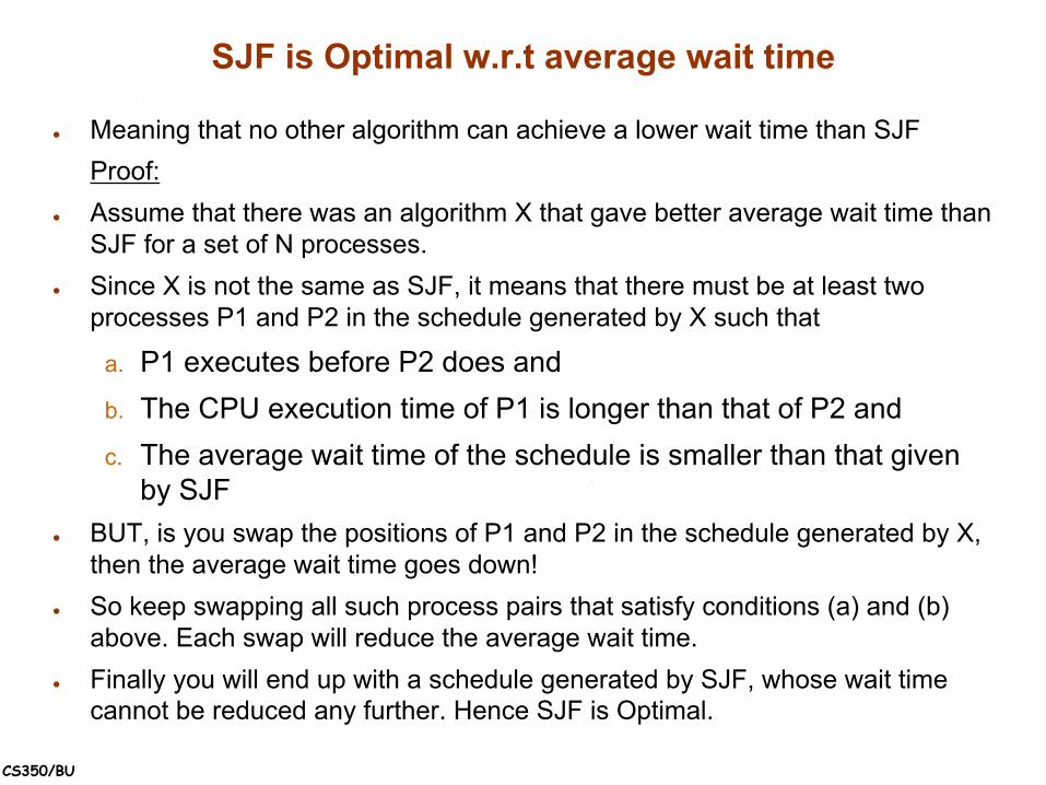
SJF is Optimal w.r.t average wait time

● Meaning that no other algorithm can achieve a lower wait time than SJFProof:

● Assume that there was an algorithm X that gave better average wait time than SJF for a set of N processes.

● Since X is not the same as SJF, it means that there must be at least two processes P1 and P2 in the schedule generated by X such that

a. P1 executes before P2 does andb. The CPU execution time of P1 is longer than that of P2 andc. The average wait time of the schedule is smaller than that given

by SJF● BUT, is you swap the positions of P1 and P2 in the schedule generated by X,

then the average wait time goes down!● So keep swapping all such process pairs that satisfy conditions (a) and (b)

above. Each swap will reduce the average wait time.● Finally you will end up with a schedule generated by SJF, whose wait time

cannot be reduced any further. Hence SJF is Optimal.

CS350/BU

Exponential Averaging:Determining the Length of Next CPU Burst

● Not easy. Can only guess the length of next CPU burst

● Can be done by using the length of previous CPU bursts, using exponential averaging

tn = actual length of the nth CPU burstτn = predicted value of the nth CPU burstα, 0 <= α <= 1Define:

τn+1 = α tn + (1-α) * τn

CS350/BU

Prediction of the Length of the Next CPU Burst

CS350/BU

Examples of Exponential Averagingτn+1 = α tn + (1-α) * τn

● α =0● τn+1 = τn

● CPU burst history does not count

● α =1● τn+1 = α tn● Only the actual last CPU burst counts

● If we expand the formula, we get:τn+1 = α tn+(1 - α)α tn-1 + …

+(1 - α )j α tn -j + …+(1 - α )n +1 τ0

● Since both α and (1 - α) are less than or equal to 1, each successive term has less weight than its predecessor

CS350/BU

Round Robin (RR)

● Each process gets a fixed unit of CPU burst time (time quantum)● usually 10 to 100 milliseconds.

● After this time has elapsed, the process is preempted and added to the end of the ready queue.

● If there are n processes in the ready queue and the time quantum is q, then each process gets 1/n of the CPU time in bursts of at most q time units at once. No process waits more than (n-1)q time units.

● Performance● q large ⇒ FIFO, because processes rarely get pre-empted● q small ⇒ Smaller response times, but too much context switching

overhead. q must be large compared to context switch time, otherwise overhead is too high

CS350/BU

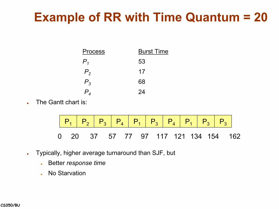
Example of RR with Time Quantum = 20

Process Burst TimeP1 53P2 17P3 68P4 24

● The Gantt chart is:

● Typically, higher average turnaround than SJF, but ● Better response time● No Starvation

P1 P2 P3 P4 P1 P3 P4 P1 P3 P3

0 20 37 57 77 97 117 121 134 154 162

CS350/BU

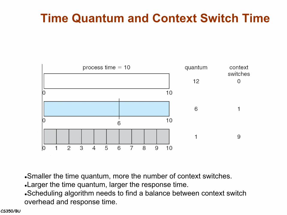
Time Quantum and Context Switch Time

●Smaller the time quantum, more the number of context switches.●Larger the time quantum, larger the response time.●Scheduling algorithm needs to find a balance between context switch overhead and response time.

CS350/BU

Priority Scheduling● A priority number (integer) is associated with each process

● The CPU is allocated to the process with the highest priority (smallest integer ≡ highest priority)

● Again two types● Preemptive● nonpreemptive

● SJF is a priority scheduling algorithm where priority is the predicted next CPU burst time

● Problem ≡ Starvation➔ low priority processes may never execute● Solution ≡ Aging➔ as time progresses increase the priority of a lower

priority process that is not receiving CPU time.

Example with four priority classes

CS350/BU

Multilevel Feedback Queue (MFQ)● Ready queue is partitioned into separate queues ● Each queue has its own scheduling algorithm ● A process can move between the various queues; ● MFQ scheduler defined by :

● number of queues● scheduling algorithms for each queue● method used to determine when to upgrade or

demote a process● Example of MFQ that gives higher priority to

interactive jobs● A new job enters queue Q0 which is served

RR.● When it gains CPU, it receives 8 ms. If it

doesn’t finish in 8 ms, job is moved to Q1.● At Q1 job is again served RR; receives 16 ms. ● If it still doesn’t complete, it is preempted and

moved to queue Q2 where it is served FCFS.

RR

RR

FCFS

Q0

Q1

Q2

CS350/BU

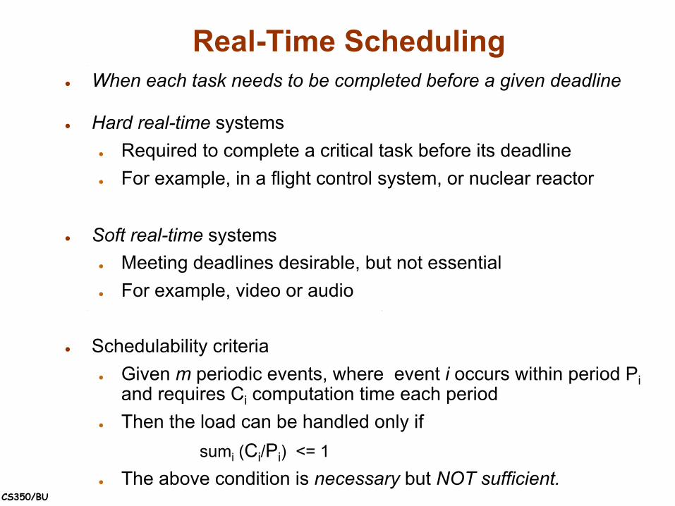
Real-Time Scheduling● When each task needs to be completed before a given deadline

● Hard real-time systems ● Required to complete a critical task before its deadline● For example, in a flight control system, or nuclear reactor

● Soft real-time systems● Meeting deadlines desirable, but not essential● For example, video or audio

● Schedulability criteria● Given m periodic events, where event i occurs within period Pi

and requires Ci computation time each period● Then the load can be handled only if

sumi (Ci/Pi) <= 1● The above condition is necessary but NOT sufficient.

CS350/BU

Fair Scheduling● Notion of “fairness” does not necessarily mean equal

CPU share for all processes.● Say you have N processes● Each process Pi is assigned a weight wi

● The the CPU time will be divided among processes in proportion to their weights.

● Let's say some process does not use its assigned CPU time.● The the “spare” CPU time is divided among the

remaining ready processed according to the ratio of their weights.

CS350/BU

Work-conserving versus non-work-conserving

● Work-conserving scheduler● CPU will not remain idle if there are processes

in the ready queue

● Non-work-conserving scheduler● Under some conditions, scheduler may decide

to “waste” CPU time even though there may be processes sitting in the ready queue

● E.g. Sometimes real-time process cannot be started before a given time (release time).

CS350/BU

Linux CPU Scheduling Code

To browse, go to http://lxr.linux.no/

To download, modify, and compile, go to

http://ftp.kernel.org/

Scheduling code is located under

kernel/sched.c

Entry points into the kernel are located at

arch/x86/entry_32.SOR arch/x86/entry_64.S