CPPI strategies and the problem of long-term guaranteesoops.uni-oldenburg.de/2743/1/tsacpp16.pdf ·...

CPPI strategies and the problem oflong-term guarantees

Von der Fakultat fur Mathematik und Naturwissenschaften der Carl von OssietzkyUniversitat Oldenburg zur Erlangung des Grades und Titels eines

Doktors der Naturwissenschaften (Dr. rer. nat.)

angenommene Dissertation

von Frau Yi-Ting Tsai

geboren am 9. Juli 1984 in Chiayi, Taiwan

Gutachterin: Prof. Dr. Angelika MayZweitgutachter: Prof. Dr. Dietmar Pfeifer

Tag der Disputation: 15.03.2016

Abstract

Due to the incomplete downside-risk protection possessed by portfolio insurance strate-gies, we are particularly interested in one of the most classical ones: Constant ProportionPortfolio Insurance (CPPI), and the consequential risk its issuers confront with based onthe unfulfilled guarantee.

In the thesis we propose a new model for the risky asset dynamic concerning the gap risk,and further loosen the traditional restriction in the CPPI strategies with regard to the non-risky asset, which is constantly assumed to evolve with riskfree rate. The cushion dynamicis under the new framework driven by a bivariate Levy process, the solution to the stochas-tic differential equation is a generalized Ornstein-Uhlenbeck process. Hence we are able toderive explicitly the risk measures through stochastic integration.

Empirical results are also provided in the end of the thesis. We compare the simulationoutcome from the new model with Kou and Merton models, along with their performancesinside the CPPI portfolio.

i

Zusammenfassung

Verschiedene Portfolio Insurance Strategien weisen eine unvollstandige Absicherung gegen-uber dem Downside-Risiko auf. Hier wird eine der klassischen Strategien untersucht, dieConstant Proportion Portfolio Insurance-(CPPI-)Strategie, vor allem im Hinblick auf dasresultierende Risiko fur die Emittenten, das aus nicht erfullten Garantien entsteht.

In dieser Dissertation stellen wir ein neues Modell fur die riskante Dynamik von Assetsvor, welches auch Gap-Risiko berucksichtigt und außerdem lockern wir die klassische Ein-schrankung der CPPI-Strategien fur nicht-riskante Assets, grundsatzlich eine Asset-Entwick-lung mit risikolosem Zinssatz anzunehmen. Nach diesem neuen Ansatz wird die Cushion-Dynamik von einem bivariaten Levy-Prozess gesteuert. Die Losung der zugehorigen stochasti-schen Differentialgleichung ist ein verallgemeinerter Ornstein-Uhlenbeck-Prozess. Daherkonnen wir die Risikomaße mit stochastischer Integration herleiten.

Am Ende dieser Dissertation werden empirische Ergebnisse dargestellt. In einer Simulationvergleichen wir das neue Modell mit den Modellen von Kou und Merton und ihre Perfor-mance im CPPI-Portfolio.

iii

Acknowledgements

The completion of this thesis could not have been possible without the support from myadviser, Prof. Dr. Angelika May. I appreciate the opportunity to work and study under herguidance, and all the wise advices and encouragement she had kindly given me. The admi-ration to my second adviser, Prof. Dr. Dietmar Pfeifer, is beyond words. His intelligenceand the passion for knowledge pushed me forward along the way. My sincere gratitude toerudite Prof. Dr. Peter Ruckdeschel, not only for taking part in the committee, but also forthe fruitful suggestions that he had given me, either for my thesis or for my future career.

Many thanks are dedicated to my colleagues who have accompanied me through highs andlows: Andreas and Herve, those coffee and tea we drank together these years have finallyturned into this work, I am truly grateful. The discussion with Kornelius at the final stageof my thesis in the matter of improvement was of special help to me.

Without my dearest friends here I would not have pulled my life as a PhD student through:Lena, my hero, in her I see a true friend and I look up to her. I cannot thank her enoughin my life for her generosity. Jorg, my dear friend who showed me the kindness of Germansduring my first visit, makes me fall in love ever since with this beautiful country, Germany.Yu-Chuan, my savior, her existence in a foreign country is already an enormous comfort forme. Mensa-Gang: Melanie, Sinje, Sven and Thomas, the support I gain from them makesme strong enough to cope with every situation I confront with. My deepest gratitude tothese friends, who are practically my families here.

Last but not least, I thank my families, Yun-Fu and friends in Taiwan genuinely, who makeme realize where my root is. Without their love and support I would not have come this far.

v

Contents

Abstract i

Zusammenfassung iii

1 Introduction 1

2 Preliminaries 52.1 Stochastic Processes and Semimartingales . . . . . . . . . . . . . . . . . . . . 5

2.2 Stochastic Integration . . . . . . . . . . . . . . . . . . . . . . . . . . . . . . . 6

2.3 Levy process . . . . . . . . . . . . . . . . . . . . . . . . . . . . . . . . . . . . 8

2.4 Cumulants . . . . . . . . . . . . . . . . . . . . . . . . . . . . . . . . . . . . . . 11

3 Stochastic Model without Gap Risk Assumption 15

4 Stochastic Model Concerned with Gap Risk 174.1 Model Setup for the Risky Asset . . . . . . . . . . . . . . . . . . . . . . . . . 18

4.2 Model Setup for the CPPI Strategy . . . . . . . . . . . . . . . . . . . . . . . . 21

4.2.1 When Yield Does Not Coincide with Money Market Return . . . . . . 21

5 Measuring the Gap Risk 275.1 Probability of Loss . . . . . . . . . . . . . . . . . . . . . . . . . . . . . . . . . 27

5.2 Expectation of Loss . . . . . . . . . . . . . . . . . . . . . . . . . . . . . . . . 29

5.3 Variance of Loss . . . . . . . . . . . . . . . . . . . . . . . . . . . . . . . . . . 33

5.4 Value at Risk and Conditional Value at Risk . . . . . . . . . . . . . . . . . . 38

6 Parameter Calibration and Simulation 436.1 Estimation Methods . . . . . . . . . . . . . . . . . . . . . . . . . . . . . . . . 43

6.1.1 Maximum Likelihood Estimation . . . . . . . . . . . . . . . . . . . . . 43

6.1.2 Empirical Characteristic Function Method . . . . . . . . . . . . . . . . 44

6.1.3 Cumulant Matching Method . . . . . . . . . . . . . . . . . . . . . . . 46

6.2 Numerical Implementation . . . . . . . . . . . . . . . . . . . . . . . . . . . . . 49

6.3 Forecasting Ability . . . . . . . . . . . . . . . . . . . . . . . . . . . . . . . . . 58

7 Conclusion 63

Appendices 65

vii

List of Figures 85

List of Tables 86

List of Notation 89

Bibliography 91

Curriculum Vitae 97

Lebenslauf 99

viii

1 | Introduction

European Central Bank reduced its benchmark interest rate on June 2014 to −0.1%, andup to December 2015 the interest rate has been further cut to −0.3% ([ECB, 2015]). Partic-ular interest is therefore drawn to investment strategies since the riskfree investments willnot contribute much to the capital for investors. For instance, capital protection strategiesprovide the investors an occasion to participate in the long term return provided by riskyinvestments, and at the same time limit the risk of loss.

CPPI, as the most basic form of portfolio insurance strategy, is the approach on which welay our eyes in the thesis. The aim of the strategy is to protect the investors from marketrisk through guaranteeing them a certain percentage of the initial capital investment. Port-folio value is contributed from two sorts of investments, one in the risky asset equal to theproduct of a constant multiplier and the cushion, which is the difference between the currentportfolio value and the guaranteed amount; the other in the non-risky asset. Leverage istherefore created from this multiplier so as to increase the position in the risky asset (SeeChapter 3 for further detail). Thus, the setup results in a buy high sell low strategy. It canbe further customized to meet investors’ needs with respect to the individual risk preference,e.g. the level of leverage and the guarantee level.

CPPI was introduced by [Black and Jones, 1987] as an alternative method to allocate in-vestments dynamically between risky and non-risky assets over a time horizon. Since then,several comparisons between CPPI and other portfolio insurance strategies have been inves-tigated. For example, the comparison between CPPI and other dynamic strategies: Buy-and-hold, constant mix and Option Based Portfolio Insurance (OBPI) was given in [Peroldand Sharpe, 1988] with respect to the payoff and exposure diagrams. Later, [Bertrandand Prigent, 2005] analyzed OBPI and CPPI in accordance to their payoffs at maturity,stochastic dominance of their returns. Dynamic hedging properties were also examined, inparticular classical delta hedging. [Lin and Shyu, 2008] and [Joossens and Schoutens, 2008]provided overviews on the differences between time invariant portfolio protection, ConstantProportion Debt Obligation (CPDO) and CPPI, respectively. More recently, the perfor-mance of the CPPI and OBPI strategies was analyzed by [Bertrand and Prigent, 2011] usingOmega measure, which was first introduced by [Keating and Shadwick, 2002], under whichthe CPPI method outperformed the OBPI.

The properties of continuous-time CPPI strategies have also been studied extensively inthe literature, cf. [Black and Perold, 1992] investigated the effect of transaction costs andborrowing constraints on the strategy. An extension for CPPI was provided in [Prigent andTahar, 2005] with an additional insurance on the cushion. Furthermore, a discrete-time ver-sion of the continuous-time CPPI strategy was proposed by [Balder et al., 2009], in which the

2 Chapter 1. Introduction

trading was restricted to discrete time. The result was further extended by [Weng, 2014],in which a double-sided Laplace inversion method was developed to compute the Omegameasure of a CPPI portfolio.

Despite its name, the insured portfolio in practice is not typically literally insured, which isthe reason encouraging us to assess the risk encountered. On one hand, risky asset in thestrategy has often been assumed under the scheme of [Black and Scholes, 1973], which hadbeen shown that CPPI strategies under such a model setup never result in violation of theguarantee; on the other hand, heavy-tailed returns of the risky asset are widely recognizedand empirically observed in the financial market, e.g. [Borak et al., 2010]. These facts ren-dered a spur to research on jump-diffusion models, which was firstly introduced by [Merton,1976].

An amount of empirical and theoretical research proved the existence of jumps and their sub-stantial impact on financial management. In the case of pricing and hedging, since [Merton,1976] derived an option pricing formula when the underlying stock returns are generated bya mixture of both continuous and jump processes, research on alternative models due to vari-ous distributed jumps has boosted, cf. [Ramezani and Zeng, 1998] proposed the Pareto-Betajump-diffusion model, assuming that good and bad news are generated by two independentPoisson processes and jump magnitudes are drawn from the Pareto and Beta distributions.[Kou, 2002] proposed another model whose jump is characterized by an asymmetric doubleexponential distribution, and later demonstrated the result of option pricing with regard toAmerican options in [Kou and Wang, 2004]. For European option pricing, see e.g. [Escobaret al., 2011]. [Cai and Kou, 2011] extended the analytical tractability of the Black-Scholesmodel to alternative models with arbitrary jump size distributions, such as Gamma, Pareto,and Weibull.

In the case of portfolio and risk management, [Cont and Tankov, 2009] studied the behaviorof CPPI concerning the price jumps and derive various associated risk measures in the con-text of a jump-diffusion price process, along with the problem of downside-risk hedging byusing options. Later for another structured credit derivative CPDO, [Cont and Jessen, 2012]gave a thorough risk analysis of the strategy by using a top-down approach and obtainedthe numerical results by Monte Carlo method. The capital requirement for a long-tern guar-antee under the framework of Solvency II with respect to the different risk measurementswas discussed in [Devolder, 2011]. [Weng, 2013] investigated the CPPI portfolio under somepopular Levy models from Merton, Kou, variance gamma and normal inverse Gaussian mod-els. The OBPI strategy which minimizes the Value-at-Risk (VaR) of the hedged position ina continuous time, regime-switching jump-diffusion market was investigated by [Ramponi,2013]. [Pezier and Scheller, 2013] concluded CPPI strategies still outperformed OBPI onesunder the consideration of gap risk.

In order to implement the theoretical models into practice, parameter calibration for theempirical data is the next aim. Maximum Likelihood Estimation method (MLE) is one ofthe most widely implemented estimation methods, which produces the most efficient param-eter estimates. This is, however, only possible when the likelihood function is in a tractableform. Alternative techniques are proposed so as to cope with such difficulties arising fromthe likelihood function.

Due to the one-to-one correspondence between the distribution functions and the characteris-tic functions, Empirical Characteristic Function method (ECF) is one of the desirable meth-

3

ods while estimating. The original idea of this estimation method was initialized by [Parzen,1962], and later obtained major theoretical support in the works from [Feuerverger andMureika, 1977], [Feuerverger and McDunnough, 1981] and [Feuerverger, 1990] with asymp-totic efficiency results and block approach for stationary time-series. The basic idea behindthe method is to minimize the weighted difference between the empirical and theoreticalcharacteristic functions. Various weighted functions have been investigated due to the re-search from [Feuerverger and Mureika, 1977], cf. [Jiang and Knight, 2002], Chacko andViceira [2003].

Moreover, [Carrasco and Florens, 2000] concluded that continuous ECF estimator can beseen as a special case of the generalized method of moments with a continuum of momentconditions. An overview of the ECF method and its application on affine jump-diffusionmodels was provided by [Yu, 2004]. More recently, [Levin and Khramtsov, 2015] consideredthe method for estimating parameters of affine jump-diffusions with unobserved stochasticvolatility.

The aim of this thesis is to construct a stochastic model for the self-financing CPPI strategyunder the continuous-time framework. Furthermore, the gap risk and its resulting effect onthe strategy are taken into consideration. In the light of the above objectives, the thesis isoutlined as follows.

In Chapter 2 an overview on the prerequisite tools in the field of stochastic analysis which weimplement throughout the thesis is provided. Particularly in this chapter we refer to [Sato,2005], [Protter, 2005], [Applebaum, 2009] and references therein for general theory on Levyprocesses and stochastic integration, and [Cont and Tankov, 2004] and [Pascucci, 2011] fortheir applications in finance modeling.

The following chapter is dedicated to the CPPI strategy under the classical framework - theBlack-Scholes model. We first clarify the mechanism behind the strategy, in which the riskyasset is described as a geometric Brownian motion. From the closed-form expression of thevalue process, it is foreseeable the model is not adequate for risk assessment.

In order to deal with the impractical problem we face in the former chapter, we includethe gap risk in the dynamic of the risky asset in Section 4.1. We start from reviewing thefeatures of well-known Merton and Kou models, respectively. According to the result of datafitting we propose a new model with a different jump characteristic in order to capture moreaccurately the sudden jumps of market prices and to get a better characterization under themathematical framework.

Apart from the modification of the price dynamic in risky asset, in Section 4.2 we furtherrelax the restriction of the CPPI strategy on the non-risky investment, which does not nec-essarily evolve from the riskfree rate anymore, yet it can be chosen from a pool of financialproducts with higher yields. Based on this new setup in the CPPI strategy, we derive aclosed-form solution to the cushion in the end of this chapter, as well as the solution to theportfolio value.

Chapter 5 focuses on the effect of modified CPPI strategies on statistical evaluation andvarious risk measures, which allows the portfolio insurance issuers to further assess the ex-tent of risk they confront with. The results from Section 5.1 and 5.1 are derived based onthe the former chapter and the moments of Doleans-Dade exponential. In terms of VaR andConditional VaR (CVaR) we use the inverse Fourier transform to retrieve the distribution

4 Chapter 1. Introduction

function.

Empirical data from various assets in major markets are implemented in Chapter 6. Sec-tion 6.1 illustrates the estimation results from Chapter 4 with regard to the jump-diffusionmodels. Parameters are estimated from daily log-returns with ECF and MLE methods,which are reviewed in Section 6.1. Additionally, we combine the two estimation methods tocalibrate the parameter. Two sources of initial values are also provided. Overall, parameterfrom each asset is estimated in 6 different ways for each model. With the help of Q-Q plotsand Akaike Information Criterion (AIC) we compare the performances among Kou, Mertonand our new models with respect to different estimation methods in Section 6.2.

After modifying the dynamic of the risky asset we are interested to see how it unfolds andif it further possesses the forecasting ability. The analysis is done by out-of-sample testingwith respect to the performance of the CPPI strategy. The result and the comparison toother models are demonstrated in Section 6.3.

2 | Preliminaries

In this chapter a few preliminaries in stochastic analysis will be introduced. A completeprobability space (Ω,F ,P) is assumed to be given throughout the thesis. Furthermore thisprobability space will be provided with a filtration Ftt≥0, which is an increasing sequenceof σ-algebras with Ft ∈ F , ∀t ≥ 0, to obtain a filtered probability space (Ω,F , Ftt≥0,P).

In addition, the filtered probability space is said to fulfill the usual hypotheses if it is complete,i.e. F0 contains all the P-null sets, and right continuous, i.e. Ft+ =

⋂s>tFs is equal to Ft

for all t ≥ 0. Note that we assume the usual hypotheses are satisfied in this thesis.

Section 2.1 will give a brief overview to stochastic processes, and then the focus will be seton a special class of stochastic processes called “semimartingales”, which is the key to thetopic stochastic integration in the next section. Attention will move on to Levy processesin Section 2.3. From Levy-Ito decomposition we are able to see the relation between Levyprocesses and semimartingales.

2.1 Stochastic Processes and Semimartingales

A stochastic process X on (Ω,F ,P) is a collection of real-valued random variables Xtt≥0. Xis said to be an adapted process if Xt ∈ Ft, ∀t ≥ 0, which means Xtt≥0 is non-anticipatingwith respect to the information structure Ftt≥0. The filtration which is generated bythe past values of the stochastic process X is called a natural filtration F0

t t≥0. Thatis, F0

t t≥0 is the smallest filtration that makes X adapted. One can obtain the so-calledaugmented natural filtration by extending the natural filtration such that it satisfies the usualhypothesis.

Moreover, a stochastic process is said to be cadlag if it almost surely (a.s.) has sample pathswhich are right continuous (continue a droite), with left limits (limite a gauche). Similarly, astochastic process X is said to be caglad if it a.s. has sample paths which are left continuous,with right limits.

An adapted stochastic process Mtt≥0 is said to be a martingale with respect to the filtrationFtt≥0, if E [|Xt|] <∞ for all t ≥ 0, and E [Xt|Fs] = Xs a.s. for 0 ≤ s ≤ t.

Next we introduce stopping time as a random variable τ : Ω → [0,∞) which fulfills thefollowing condition: Event τ ≤ t ∈ Ft, ∀t > 0, i.e., event τ ≤ t is Ft-measurable,for each t. And then we define the “good integrators” on an appropriate class of adaptedprocess, that is, semimartingale, which later will be used in our model setup.

6 Chapter 2. Preliminaries

Definition 2.1.1. (Local Martingale) An adapted stochastic process X is a local martin-gale if there is a sequence of increasing stopping times τnn>0 with lim

n→∞τn =∞ a.s. such

that Xt∧τnt≥0 is a martingale for each n.

Definition 2.1.2. (Semimartingale) An adapted stochastic process X is called a semi-martingale, if it can be written as the following form

Xt = X0 +Mt +At,

where M is a local martingale and A is a process that has finite-variation.

2.2 Stochastic Integration

In the process of deriving the explicit solutions to risk measures in Chapter 5, some stochas-tic integrals driven by semimartingales need to be overcome. Therefore we will give anintroduction regarding the stochastic integration, which was initially developed by Ito withrespect to the standard Brownian motion.

We introduced in the last section the “good integrators”, now we wish to know the processeswe can consider as integrands.

Definition 2.2.1. (Simple predictable process) A stochastic process H is called a simplepredictable process if it can be represented as

Ht = H010(t) +n∑i=1

Hi1(τi,τi+1](t),

where τ0 = 0 < τ1 < τ2 < ... < τn < τn+1 < ∞ is a finite sequence of stopping times,Hi ∈ Fτi with |Hi| <∞ a.s., 0 ≤ i ≤ n.

The stochastic integral of the simple predictable process H with respect to a stochasticprocess X is defined as

IX(H) =

∫ t

0HdX = H0X0 +

n∑i=1

Hi(Xτi+1∧t −Xτi∧t),

where IX : S → L0 is a mapping. And S represents the space of simple predictable processes,whereas the space of finite-valued random variables is denoted by L0 .

We should notice here the mapping IX has to hold for bounded convergence in probability.That is, if Hnn≥0 is a sequence of predictable processes converging to a process H anduniformly bounded, then the stochastic integral converges in probability.

sups≤t|IXs (Hn)− IXs (H)| → 0

Otherwise, a very small difference in the integrand can cause a large change in the resultingintegral. It is therefore preferable to have this property, especially in the aspect of the imple-mentation in finance. This class of stochastic process X is the mentioned “good integrators”

2.2. Stochastic Integration 7

- semimartingales. Moreover, we can analogously enlarge the space of possible integrands,e.g. locally bounded predictable integrands (For details please refer to [Protter, 2005]). Inaddition, the stochastic integral of an adapted process H with respect to a semimartingaleis, by Definition 2.1.2, the sum of two integrals, one with respect to the local martingale andthe other with respect to the finite variation process, which can be calculated path by pathas the Stieltjes integral.

In the rest of this section we give some important extensions of stochastic integrals whichwill be used frequently throughout this thesis.

Definition 2.2.2. (Quadratic covariation) Given two semimartingales Xt and Zt, thequadratic covariation process [X,Z]tt≥0 is the semimartingale defined by

[X,Z]t = XtZt −X0Z0 −∫ t

0Xs−dZs −

∫ t

0Zs−dXs

The quadratic covariation is alo called the bracket process. Its definition leads us to thestochastic integration by parts formula. Next we present the Ito-Doblin theorem for a specialcase: semimartingales. It explains the structure of a process f(X) given a “nice” functionf .

Theorem 2.2.1. (Ito-Doblin theorem for semimartingales) Given a semimartingaleX and f be a C2 function of X. Then f(X) is also a martingale and written in the followingform

f(Xt) =f(X0) +

∫ t

0f ′ (Xs−) dXs +

1

2

∫ t

0f ′′ (Xs−) d[X,X]cs

+∑

0<s≤t

f (Xs)− f (Xs−)− f ′ (Xs−) ∆Xs

Proof See [Protter, 2005], Theorem II.32.

One of the applications from Ito-Doblin Theorem is the derivation of the solution to

dZ = Z−dX

If X is a deterministic process, e.g. Xt = t, the solution is given as a exponential function.However, if X and Z are two semimartingales, the solution to it is given in the followingtheorem.

Theorem 2.2.2. (Doleans-Dade exponential) Let X be a semimartingale. There existsan unique semimartingale Ztt≥0 such that

dZt

Z−t= dXt, Z0 = 1

which is called stochastic or Doleans-Dade exponential of X, denoted by E(X)t and writtenexplicitly as

Zt = E(X)t = eXt−X0− 12

[X,X]ct∏

0<s≤t(1 + ∆Xs) e

−∆Xs

Proof See [Cont and Tankov, 2004], Proposition 8.21.


2.3 Levy process

Another popular class of stochastic processes will be presented in this section, the Levy pro-cess. Again, a filtered probability space (Ω,F , Ftt≥0,P) is given and the usual hypothesisis fulfilled.

Definition 2.3.1. (Levy process) A cadlag stochastic process Xtt≥0 with X0 = 0 a.s.is called a Levy process if it possesses the following properties:

1. Independent increments: for every increasing sequence of times t0, t1, ..., tn, the ran-dom variables Xt1 −Xt0, Xt2 −Xt1, ... , Xtn −Xtn−1 are independent

2. Stationary increments: ∀h > 0, the distribution of Xt+h −Xt does not depend on t

3. Continuity in probability: ∀ε > 0, limh→0

P (|Xt+h −Xt| > ε) = 0

Further information can be found in [Protter, 2005] and [Cont and Tankov, 2004].

The most elementary and well-known jump process is the homogeneous Poisson process.Before any further detail is given, we should first have some basic concept of the countingprocess, denoted by Ntt≥0. The value of the process is given by

Nt =

∞∑k=1

1[Tk,∞)(t), t ∈ R+

∆NTk = NTk −NTk− = 1,

where Tkk∈N represents the time when jumps occur. If the random times Tkk∈N arepartial sums of i.i.d. exponential random variables, then Ntt≥0 is a homogenous Poissonprocess if it satisfies the following properties:

1. Independent increments: for all 0 < t0 < t1 < ... < tn, n ∈ N, the random variablesNt1 −Nt0 , Nt2 −Nt1 , ... , Ntn −Ntn−1 are independent

2. Stationary increments: for all h > 0, 0 ≤ u < t, Nt+h−Nu+h has the same distributionas Nt −Nu

Proposition 2.3.1. The homogeneous Poisson process is a Levy process

The homogeneous Poisson process defined above counts events that occur at a constant rate.Moreover, Nt−Nu follows the Poisson distribution with parameter λ(t− u). Therefore, theexpected value of Nt is

E[Nt] = λt

Obviously the homogeneous Poisson process has its own restrictions to describe the behaviorof the asset price jumps. Thereby we introduce another more general process: compoundPoisson Process so as to mimic the asset price jumps better.

Define Jkk∈N as a sequence of i.i.d. random variables with probability distribution πand independent of the Poisson process Ntt≥0 whose intensity rate is λ. The followingdefinition is obtained.

2.3. Levy process 9

Definition 2.3.2. The process Ytt≥0 which is given as

Yt =

Nt∑k=1

Jk

is called a compound Poisson process

Proposition 2.3.2. The compound Poisson process is a Levy process

By construction, Ytt≥0 has paths that are constant apart from a finite number ofjumps in any finite time interval. In comparison to the counting process Ntt≥0, the jumpsof Ytt≥0 occur at the same time as the jumps of Ntt≥0. The only difference is the jumpsof Ntt≥0 are always of size 1, whereas the jumps of Ytt≥0 are of random size.

Proposition 2.3.3. The characteristic function of a compound Poisson process Ytt≥0 withintensity λ is

E[eiuYt

]= eλt

∫∞−∞(eiuy−1)π(dh)

The first and second moments are therefore derived as follows:

E [Yt] = λtE [J1] and Var [Yt] = λtE[J1

2]

Proof The moments can be attained by Proposition 2.4.1. Or we can prove it either by usingthe characteristic function or by the law of total expectation. The characteristic functioncan also be derived easily

E[eiuYt

]=

∞∑n=0

E

(eiu

n∑k=1

Jk

)P (Nt = n)

=∞∑n=0

e−λt (λt)n

n!E

(eiu

n∑k=1

Jk

)

=

∞∑n=0

e−λt (λt)n

n!

[E(eiuJ1

)]n= e−λt

∞∑n=0

[λtE

(eiuJ1

)]nn!

= eλt[E(eiuJ1)−1]

= eλt∫∞−∞(eiuy−1)π(dy)

For the expectation, we have

E [Yt] =1

i

(d

duE[eiuYt

]|u=0

)= λt

∫ ∞−∞

yπ(dy)

= λtE [J1]

The variance can hereby be derived.


Definition 2.3.3. The process Mtt≥0 with Mt := Nt−λt is called a compensated Poissonprocess, where Ntt≥0 is a counting process and λ is its intensity.

Now that we have reviewed the commonly used processes which describe pure jumps, wewould like to focus on the Levy processes which possess jumps, and how it can be charac-terized. To each cadlag stochastic process Xtt≥0 on R, one can associate jump measureJX with Xtt≥0 as follows:

JX(B) = #(∆Xt, t) ∈ B,∀B ∈ B(R× [0,∞))

where ∆Xt = Xt −Xt− .

In a period of time, e.g. [t1, t2], the jump measure JX(A × [t1, t2]) counts the number ofjumps of X whose jump sizes are in A ∈ B(R) between the time t1 and t2. If Xt is acompound Poisson process with intensity λ and jump size distribution π, then the jumpmeasure of which is a Poisson random measure with intensity measure λπ(dx)dt = ν(dx)dt,where ν is the Levy measure which will be shown in the next definition.

From the interpretation of the intensity measure of a compound Poisson process, it is clearto see that its Levy measure can be seen as the average number of jumps per unit of time.And this holds for all Levy processes.

Definition 2.3.4. Let Xtt≥0 be a Levy process on R. The measure ν on R defined by

ν (A) = E [#t ∈ [0, 1] : ∆Xt 6= 0,∆Xt ∈ A] , A ∈ B (R)

is called the Levy measure of X: ν (A) is the expected number, per unit time, of jumps wheresizes belong to A.

If a Levy process has only a finite number of jumps in any bounded time interval (e.g.compound Poisson process) we say that it is a finite activity Levy process. Otherwise we saythat it has infinite activity, which means that singularities, i.e. infinitely many jumps, canoccur around the origin. Moreover, the jump mass away from the origin of a finite activityLevy process is bounded, i.e. only a finite number of big jumps can occur. One of most wellknown models that deals with finite activity Levy processes is the Merton jump-diffusionmodel [Merton, 1976], which is the independent sum of a Brownian motion with drift and acompound Poisson process.

In order to cope with the convergence problem when it comes to infinite activity, every Levyprocess can be represented in the following form.

Theorem 2.3.1. (Levy-Ito decomposition) Let Xtt≥0 be a Levy process on R withjump measure J and Levy measure ν fulfilling∫

|x|>1ν (dx) <∞ and

∫|x|≤1

x2ν (dx) <∞

For any R > 0 we can write Xt into the sum of independent Levy process X(1)t , X

(2)t and

X(3)t where

1. X(1)t = µRt + σWt, which is a Brownian motion with drift, where µS = µR −∫S<|x|≤R xν (dx)

2.4. Cumulants 11

2. X(2)t =

∫ t0

∫|x|≥R xJ(dx, ds) =

∑0<s≤t

∆Xs1|∆Xs|≥R, which is a compound Poisson

process that is responsible for the large jumps

3. X(3)t =

∫ t0

∫ε≤|x|<R xJ(dx, ds) =

∑0<s≤tε≤|x|<R

∆Xs − tE[∆X11ε≤|∆Xs|<R], which is a

L2-martingale that deals with the small jumps and ε→ 0+

Definition 2.3.5. (µR, σ2, ν) is called the Levy R-triplet of a Levy process X.

In most of the literature it can be found that the choice of R = 1 is common. And ifthe process has finite activity, we no longer need to truncate the small jumps, the jump partcan actually separated from the continuous part of the process by setting R go to zero. TheLevy triplet for finite activity Levy process is (µ0, σ

2, ν), where

µ0 = µ1 −∫

0<|x|≤1xν (dx) ,

which has an intrinsic interpretation as the continuous part of the process, whereas µ1

depends on the truncation function.

In the next section we can observe that, according to the Levy-Ito decomposition it followsthat all Levy processes are semimartingales with respect to the augmented natural filtration.

Theorem 2.3.2. (Levy-Khintchine representation) Let Xtt≥0 be a Levy process onR with Levy triplet (µ1, σ

2, ν) Then

E[eiθXt

]= etψ(θ), θ ∈ R

where the Levy exponent

ψ (θ) = iµ1θ −1

2σ2θ2 +

∫R

(eiθx − 1− iθx10<|x|≤1

)ν(dx) (2.1)

Note that the conditions on the Levy measure are sufficient to ensure that the integralin (2.1) converges since the integrand is O(1) for |x| > 1 and O(x2) for |x| ≤ 1.

In the case of finite activity the equation (2.1) can be simplified as

ψ (θ) = iµ0θ −1

2σ2θ2 +

∫R

(eiθx − 1

)ν (dx)

2.4 Cumulants

The Levy-Khintchine formula allows us to compute easily the cumulants of a Levy process.In the thesis, cumulants are also used in deriving the closed-form solutions to risk measures.Furthermore, we also use them to locate a set of reasonable initial values for parametersestimation.


Definition 2.4.1. The characteristic function of the random variables X, with values in R,is the function φX : R→ C defined by

φX(u) = E[eiux], u ∈ R

=

∫ReiuxPX(dx), u ∈ R

φX is simply the Fourier transform of the distribution PX of X. In particular, if PX hasa density f , then we write φX = F (f). In addition, if X ∈ Lp, then

m′p = E[Xp] =

1

ipdp

dupφX(u)|u=0

is called the p-th moment of X, whereas

mp = E[(X − E[X])p]

is called the p-th central moment of X.

Since φX(0) = 1 and φX is a continuous function, it can be proved in Lemma 7.6 in [Sato,

2005] that there exists a unique continuous function ψX such that φX(u) = eψX(u) andψX(0) = 0. The function ψX is called the cumulant generating function of X, and alongwith it is the cumulants of X defined as follows:

cn(X) =1

indn

dunψX(u)|u=0

Differentiating the cumulant generating function, for instance, results in

c1(X) = E[X]

c2(X) = Var(X)

The relation between cumulants and central moments is the key to the Cumulant MatchingMethod (CMM), which will be further discussed in Section 6.1.3.

Proposition 2.4.1. Let X be a Levy process on R generated by Levy triplet (µ1, σ2, ν). The

n-absolute moment E[|Xt|n] is finite if and only if∫|x|≥1

|x|nν(dx) <∞

In particular, we have

cn(Xt) = tcn(X1), n ≥ 1

Proof See [Pascucci, 2011], Proposition 13.45

Proposition 2.4.2. Let X be a Levy process on R. If E[|X1|] <∞, then

Xt − E [Xt]

is a martingale.

2.4. Cumulants 13

Proof Since E[Xt] = tE[X1] from Proposition 2.4.1, and if E[|X1|] <∞, then Xt −E[Xt] isintegrable. Moreover, by the independence of increments we have

E[(Xt − E[Xt])− (Xs − E[Xs]) | Fs] = E[Xt −Xs | Fs]− E[X1](t− s)= E[Xt−s]− E[X1](t− s)= 0

and therefore Xt − E[Xt] is a martingale.

Corollary 2.4.1. The compensated Poisson process followed by Definition 2.3.3 is a cadlagmartingale with respect to the filtration Ftt≥0.

3 | Stochastic Model without Gap RiskAssumption

The theoretical background introduced in the preceding chapter enables us to describe thedynamic of the CPPI portfolio by using continuous-time stochastic processes. In this chapterwe introduce the classical setup of the portfolio, in which the gap risk is omitted.

CPPI is a dynamic portfolio insurance strategy which provides downside protection for theportfolio by setting up a threshold to the portfolio value. The protection is obtained byreallocating the exposure to the risky asset based on the surplus to the discounted guarantee.Throughout the thesis we assume a self-financing CPPI portfolio in a frictionless market.

The portfolio constructed under the CPPI framework consists of two parts of investments.One part in non-risky asset, say B, which evolves with a riskfree rate r ; and the other inrisky asset, S, a geometric Brownian motion with µ and σ as the expected rate of return andthe volatility of S, respectively. µ, σ ∈ R.

The classical dynamics of B and S are given as follows

dBt = rBtdt

dSt = µStdt+ σStdWt

The Guarantee of the CPPI portfolio is assumed to be G. It is the least payment the investorshould receive at maturity T. Set Pt to be the present value of G, discounted by the riskfreerate r, which forms the Floor.

In other words, once the Floor is violated, the Guarantee will be unfulfilled at maturity.Consequently, the insurance issuer is obligated to cover the difference between the Guaranteeand the final portfolio value. Mathematically we describe the Floor in the following way.

Pt = Ge−r(T−t)

dPt = rPtdt

Consider a CPPI portfolio whose Value is written as V, which contains B and S, we write

dVt = αtdStSt

+ (Vt − αt)dBtBt

, αt ∈ R (3.1)

The amount of money which is invested in the risky asset is denoted by αt = mCt, whereCt = Vt−Pt is the Cushion, and m is the Multiplier, which is a finite positive number. Onecan rewrite (3.1).

dVt = [rVt +m(Vt − Pt)(µ− r)] dt+m(Vt − Pt)σdWt (3.2)

16 Chapter 3. Stochastic Model without Gap Risk Assumption

Rearrange (3.2), the equation becomes

dVt = rPtdt+ (Vt − Pt) [m (µ− r) + r] dt+mσdWt

It is clear to see that the cushion process Ctt∈[0,T ] is driven by the process Dtt∈[0,T ]

dDt = [m (µ− r) + r] dt+mσdWt

Hence we get dVt = CtdDt + rPtdt

V0 = v

or dCt = CtdDt

C0 = v − P0 = v −Ge−rT

Since the risk premium is bounded, the above differential equation has an unique solution.

Theorem 3.0.1. The value of the cushion follows the following process

Ct = C0 · E(D)t = C0e

[m(µ−r)+r−m

2σ2

2

]t+mσWt (3.3)

Proof A direct result from Theorem 2.2.2.

4 | Stochastic Model Concerned withGap Risk

From the formula (3.3), the value of the continuously traded portfolio apparently will notdrop under the floor, since Ct is always positive for every t ∈ [0, T ], see for instance Figure 4.1,where the asset price is simulated from the Black-Scholes model.

Figure 4.1: CPPI on stock price simulated from Black-Scholes model

However in the real world, jumps of the asset prices would occur and are widely recog-nized. In order to characterize the gap risk, jump process, is therefore added to our modelsetup. The different asset price dynamics can be seen in Figure 4.2.

Firstly in Section 4.1 the attention is placed on the risky investment in the CPPI strategy,the theoretical backgrounds of well-known models, e.g. Merton and Kou models are beinginvestigated, and a different setup of asset dynamic is proposed by using different way tointerpret the jump. In the next Section 4.2, focus is set on relaxing the traditional restriction

18 Chapter 4. Stochastic Model Concerned with Gap Risk

Figure 4.2: The effect of jumps on asset price

on the non-risky investment in the CPPI strategy. Consequently our new model is born.

4.1 Model Setup for the Risky Asset

In this section we focus on a special case of Levy process, which is also the assumptionof risky asset dynamic in the thesis - jump-diffusion process. It is a combination of LevyProcesses, including a geometric Brownian motion and a jump described by a compoundPoisson process with random jump sizes.

Xt = µt+ σWt + Yt = Xct + Yt, (4.1)

where Xct is the continuous part of the process X, and Y is the compound Poisson process.

The differential of a function of the above process can be seen as a special case of Theo-rem 2.2.1. Due to the finite activity Y has, Theorem 2.2.1 for the jump-diffusion process(4.1) can then be simplified as

f(Xt) =f(X0) +

∫ t

0f ′(Xs−)dXc

s +σ2

2

∫ t

0f ′′(Xs−)ds+∑

0<s≤t(f(Xs− + ∆Xs)− f(Xs−)),

where dXcs = dXs −∆Xs.

Similarly we can derive Theorem 2.2.2 for the case of Levy process with finite activity as

4.1. Model Setup for the Risky Asset 19

a special case. With all conditions the same, only an extra condition:∫|x|≤1 |x|ν(dx) < ∞

added, then we have,

E(X)t = eXct−

σ2t2

∏0<s≤t

(1 + ∆Xs) (4.2)

In view of the above, we continue to introduce dynamics of assets with practical adjustmentsand look at its effect on the whole CPPI strategy. The setup of the risky asset dynamic S isdescribed as Equation (4.3) with the participation of jumps which follow a compound Poisson

process Yt =Nt∑k=1

(Jk− 1), whereas J is a sequence of i.i.d. random variables with probability

distribution π and independent of the Brownian motion W and the Poisson process N whoseintensity rate is λ.

dSt

S−t= µdt+ σdWt + dYt (4.3)

The difference between Merton and Kou models is how they describe the jumps using differ-ent distribution π. Under this setup (4.3) Merton introduced his model in 1976 with jumpsfollowing log-normal distribution [Merton, 1976]; Later in 2002, Kou proposed another modelby introducing double exponentially distributed jumps [Kou, 2002].

• Merton: X = log SS−

= log J ∼ N (µj , σ2j )

• Kou: X = log SS−

= log J has an asymmetric double exponential distribution, andthe density for X is

fX(x) = p1

η−e− |x|η− 1x<0 + (1− p) 1

η+e− xη+ 1x>0

with η−, η+ > 0, where p ≥ 0 represent the probability downward jumps occur.

In comparison with Merton model, in which only one random variable reflects downward andupward jumps, Kou model has better economical interpretation with asymmetric doubleexponential distributed jumps, which could capture better the leptokurtic feature of theempirical log return distribution, but when it comes to parameter estimation, an extraparameter can also bring inevitably computing burden.

Moreover, we modify the jumps to follow log-Gumbel distribution due to the fact that thereturns of our underlyings are mostly right-skewed, and a phenomenon we observe aftersimulating from Merton and Kou models. The number of parameters in our new modelremains the same as in Merton.

• new: X = log SS−

= log J ∼ G(α, β)

The characteristics that different types of jump possess are offered in Figure 4.3. The left sidefigure presents different distributions with the same mean and variance. Either exponentialor Gumbel distributed jump has fatter right tail than the normal distributed one. If we onlyfocus on the 5-parameter models, i.e. Merton and new model, the difference between eachother is evident based on the right side figure.


Figure 4.3: Comparison between different jumps in different distributions with samemean and variance

Note that for the sake of convergence when the process has infinite activity, it is useful tocompensate the jump process when one is applied into the dynamic of the asset. But in thisspecial case (finite activity) of the Levy-Ito decomposition, we do not need to compensate thecompound Poisson process. In other words, we separate the continuous part of the processfrom the jump part. Assume the jumps occur in Tii∈N, by the construction we have thejump in S at Ti represented as:

STi − STi− = STi− (YTi − YTi− ) = STi− (Ji − 1)

Hence STi = STi−Ji. This reveals that the Ji are the ratios of the asset price after and beforea jump, which indicates the jumps are multiplicative. This also explains why Ji−1 is used inthis thesis rather than simply Ji. The solution to the stochastic differential equation (SDE)(4.3) according to the special case (4.2) of Doleans-Dade exponential is then

St = S0e(µ− 1

2σ2)t+σWt

Nt∏k=1

Jk,

or rewrite it in the form of log-return

logStS0

= (µ− 1

2σ2)t+ σWt +

Nt∑k=1

log Jk

In the meanwhile, the dynamic of the non-risky asset B remains unchanged. Therefore forthe cushion process, we have

dCt

C−t= [r +m (µ− r)] dt+mσdWt +mdYt (4.4)

Analogously, the solution to the Equation (4.4) can be written as

Ct = C0e[r+m(µ−r)− 1

2m2σ2]t+mσWt

Nt∏k=1

(1 +m(Jk − 1))

4.2. Model Setup for the CPPI Strategy 21

4.2 Model Setup for the CPPI Strategy

In the previous section we focus on the cushion whose dynamic is driven by a Levy process.In order to move onto the main focus of this thesis, we will first introduce how the idea of thistopic was born in the beginning of this section. And then a new model is built by loosing thesetup of our current assumption, which will lead to a bivariate-Levy-process-driven cushion.

4.2.1 When Yield Does Not Coincide with Money Market Return

Most of the former models concerned with CPPI strategy consider only the riskfree ratewhen it comes to the investment in the non-risky asset. Nevertheless, according to SolvencyII framework, sovereign bonds are free of capital charges under the standard formula. Inother words, the sovereign bonds are still seen as riskfree asset, regardless the credit risk.Therefore we discard the assumption of the non-risky asset being savings in a bank, whichis to follow the riskfree rate r.

Hence when the insurance company invests in the non-risky asset while applying the CPPIstrategy, there are actually plenty of products to select from in the financial market besidesthose at the riskfree rate r. Which of the above will lead to a question: what if the yield,y, from the non-risky asset does not coincide with the riskfree rate, r? The answer to thisquestion is what we are seeking for in this section, and then further we study the effect ofthe CPPI strategy in such setup on risk measures.

The relation between y and r can be rationally assumed to be y > r, for the surplus canbe seen as a risk premium. Along with the assumption the setup of CPPI strategy isconsequently modified.

dBt = yBt−dt

dSt = µSt−dt+ σSt−dWt + St−dYt

dPt = rPt−dt

It is trivial to see the processes of the money market account and the non-risky asset areactually both continuous from the setup, the dynamic of the portfolio and the cushion arehereby described as

dVt = yPtdt+ (Vt− − Pt) [m (µ− y) + y] dt+mσdWt +mdYtdCt = (y − r)Ptdt+ Ct− [m (µ− y) + y] dt+mσdWt +mdYt

And the differential equation of the cushion becomesdCt − Ct−dDt = (y − r)Ptdt = dPt

C0 = v − P0 = v −Ge−rT

where

dDt = [m (µ− y) + y] dt+mσdWt +mdYt

The strategy of the CPPI indicates, once the violation occurs, all the money should bewithdrawn from the risky asset and immediately invested in the non-risky asset, i.e. the


cushion process stops at the time when the floor is broken through. A loss occurs, if forsome t ∈ R+, Vt < Pt, which is equivalent to the event Ct < 0. Set τ := inft > 0 : Ct < 0.In this case we can adjust the above equation according to the characteristics of CPPIstrategy as follows.

dCt − Ct−dDt = (y − r)Ptdt = dPt, if t < τ

Ct = Cτ , if t ≥ τC0 = v − P0 = v −Ge−rT

Or equivalently in terms of stochastic integrals,Ct − C0 =

∫ t

0dPs +

∫ t

0Cs−dDs, if t < τ

Ct = Cτ , if t ≥ τC0 = v − P0 = v −Ge−rT (4.5)

We can see from SDE (4.5) that the cushion is driven by a bivariate Levy ProcessDt, Ptt≥0. In order to solve the SDE (4.5), we will come across quadratic covariation be-tween different processes. Therefore, preliminary knowledge before the proof is hereby givenas follows. The solution to the SDE is derived in Theorem 4.2.1.

The result of the quadratic covariation of each process can be heuristically derived andis shown in the table below [Etheridge, 2002].

× dt dWt dNt

dt 0 0 0dWt 0 dt 0dNt 0 0 dNt

Table 4.1: Quadratic covariation for time, Brownian motion, and counting process

Next we provide the solution to our SDE (4.5) with the assistance of the above prelim-inaries.

Theorem 4.2.1. D and P followed from Equation (4.5) are both Levy processes. Define thestopping time as

τ := inft > 0 : Ct ≤ 0

and

τ∗ := minτ, T

then the unique solution to equation (4.5) is given by

Ct = Cat 1(0,τ∗](t) + Cbt1(τ∗,T ](t), t > 0, (4.6)


where

Cat = E(D)t

(C0 +

∫ t

0

[E(D)s−

]−1dPs

)= E(D)t

(C0 +G(y − r)e−rT

∫ t

0

[E(D)s−

]−1ersds

)Cbt = E(D)τ

(C0 +

∫ τ

0

[E(D)s−

]−1dPs

)= E(D)τ

(C0 +G(y − r)e−rT

∫ τ

0

[E(D)s−

]−1ersds

)

Proof Under the structure of CPPI, once the value of the portfolio at time t drops underthe floor, the investment in the risky asset is then terminated. In this case of t > τ , thevalue of the cushion shall remain to be Ct = Cτ . Therefore in this manner we need to focuson the case when t ≤ τ solely. It is hence to prove the following equation satisfying the SDE(4.5).

Ct = E(D)t

(C0 +

∫ t

0

[E(D)s−

]−1dPs

)(4.7)

Hereby we write Ct = C1t C

2t , where C1

t and C2t are both semimartingales w.r.t. the filtration

Ftt≥0

C1t = E(D)t and C2

t = C0 +

∫ t

0

[E(D)s−

]−1dPs

Using the definition of stochastic integration by parts, and the fact that dE(D)s = E(D)s−dDs,we have following equations

Ct − C0 =

∫ t

0C1s−dC

2s +

∫ t

0C2s−dC

1s +

[C1, C2

]t

=

∫ t

0E(D)s−

[E(D)s−

]−1dPs

+

∫ t

0

(C0 +

∫ s

0

[E(D)h−

]−1dPh

)E(D)s−dDs

+

∫ t

0

[E(D)s−

]−1d([E(D), P

]s

)=

∫ t

0dPs +

∫ t

0C1s−C

2s−dDs

=

∫ t

0dPs +

∫ t

0Cs−dDs

This proves that (4.7) is a solution to (4.5). And the uniqueness can be proven by TheoremV.7 in [Protter, 2005].


We can also prove it by using the result as pointed out in [Maller et al., 2009], a SDE interm of the following form

dVt = VtdUt + dLt, t ≥ 0, (4.8)

where U,L is a bivariate Levy process which is constructed from another pair of Levyprocesses ξ, η by

(UtLt

)=

−ξt +∑

0<s≤t(e−∆ξs − 1 + ∆ξs) + tσ2

ξ/2

ηt +∑

0<s≤t(e−∆ξs − 1)∆ηs − tσξ,η

, t ≥ 0,

and ∆ξt,∆ηt = ξt − ξt−, ηt − ηt− represents the jump processes of ξ, η at time t. Inaddition, there exists an unique solution to the SDE (4.8) which is given as

Vt = e−ξt(V0 +

∫ t

0eξs−dηs

), t ≥ 0. (4.9)

Equation (4.9) is also called as a generalized Ornstein-Uhlenbeck process Vtt≥0 driven bythe bivariate Levy process ξt, ηtt≥0. If ηtt≥0 is a Brownian motion, then we obtain theclassical Ornstein-Uhlenbeck process.

By definition of Doleans-Dade exponential, we know it is equivalent to write E(U)t = e−ξt .Hence Equation (4.9) can be written in terms of Doleans-Dade exponential.

Vt = E(U)t

(V0 +

∫ t

0[E(U)s]

−1 dηs

), t ≥ 0. (4.10)

Here we need to be careful with the modification in (4.10). Doleans-Dade exponential bydefinition can take non-positive values, but on the contrary e−ξt can only take positive values.Therefore the Levy measure ν oof U should have no mass on (−∞,−1], i.e. νU ((−∞,−1]) =0.

The above condition is exactly fulfilled by the setup of the CPPI strategy, since cushiondynamics stops evolving once the cushion value becomes non-positive.

Corollary 4.2.1. Stopping time τ can also be written as

τ = inft > 0 : 1 + ∆Dt ≤ 0

Moreover, by assumption, Ct = Cτ when t > τ , i.e. the value of cushion stops varyingafter time τ . In other words, the single jump at time τ that is less or equal to 1 − 1

m iscrucial to the whole risk assessment. The value of the portfolio is additionally presented inthe next corollary.

Corollary 4.2.2. The value of the portfolio is

Vt = V at 1(0,τ∗](t) + V b

t 1(τ∗,T ](t), t > 0,

where

V at = Pt + E(D)t

(C0 +

∫ t

0

[E(D)s−

]−1dPs

)V bt = ey(t−τ)

[Pτ + E(D)τ

(C0 +

∫ τ

0

[E(D)s−

]−1dPs

)]


It is clear to see from either Theorem 4.2.1 or Corollary 4.2.2, unlike the model con-structed in the end of Chapter 3, the solution to the cushion process in the Section 4 is likelyto be negative, i.e. the floor could be violated in the new set up, which is more realistic thanthe model proposed in the Chapter 3.

5 | Measuring the Gap Risk

Under the new framework of the model proposed in Section 4.2, CPPI strategy still maintainsits capital protection, but not anymore in an absolute sense due to the gap risk. Accordingto the violation of the floor we have the following two scenarios. See for instance: Figure 5.1and 5.2.

The following risk measure will be discussed respectively: probability, expectation and thevariance of loss in the aspect of cushion in Section 5.1, 5.2 and 5.3. In Section 5.4, VaR andCVaR will be investigated by using the inverse Fourier transform to acquire the probabilitydensity function.

Figure 5.1: Floor not violated: Different stock dynamics (left: up; right: fluctuate)and the performance of CPPI strategy

5.1 Probability of Loss

Corollary 4.2.1 implies that Ct ≤ 0 if and only if JNt ≤ 1− 1m . The jumps of the Levy process

D follows a compound Poisson process with the intensity described by the Levy measure intime period (0, T ]. Hence, the probability of loss for the cushion can be interpreted in theproposition below, where the jump size of 1− 1

m is excluded for general case.

However, the exclusion of 1− 1m with respect to the models mentioned in Section 4.1 is not

necessary, since the jump size follows continuous probability distribution.

28 Chapter 5. Measuring the Gap Risk

Figure 5.2: Floor violated: Dynamics of portfolio value (left) and cushion value whenthe floor is broken

Proposition 5.1.1. The cushion-driven-dynamic D is a Levy process with Levy measure ν,where the jump process is independent of the continuous one. The probability of loss for thecushion is

P (Ct < 0, t ∈ (0, T ]) = 1− e−TλP(JNt<1− 1m

)

Proof The following proof will be given based on the two equivalent events:

Ct < 0 if and only if ∆Dt < −1

Let ω be the first hitting time of Ct < 0, t ∈ (0, T ], and the cumulative density function of ωis FW (ω). Moreover, V is a counting process which counts the number of times of the event∆Dt < −1 occurring in time period (0, T ], and V ∼ Poisson(Tν ((−∞,−1))).

FW (ω) = F (W < ω)

= 1− P (W ≥ ω)

= 1− P (V = 0)

= 1− e−Tν((−∞,−1))

= 1− e−TλP(JNt<1− 1m

)

Note that the probability of loss of the portfolio is the same with the probability of loss ofcushion only when y = r. Since y is set to be greater than r, it is possible that the followingevent occurs: the portfolio value falls under the floor, nevertheless the loss is so little thatat maturity the yield from the non-risky investment “saves” the portfolio, see for instanceFigure 5.3. In this case, the probability of loss of the portfolio should be considered byusing another floor which is discounted by y as a threshold (brown line in Figure 5.3), i.e.P (Ct < Bt − Pt, t ∈ (0, T ]).

5.2. Expectation of Loss 29

Figure 5.3: Floor violated: Dynamics of portfolio value (left) and cushion value whenthe floor is broken

However, under the framework of y 6= r, Bt−Pt is negative, ∀t, which indicates that everyjump size could be the cause for a negative cushion depending on the previous cushion value.Nevertheless, the probability in Proposition 5.1.1 is still an upper bound for the probabilityof loss of the portfolio.

5.2 Expectation of Loss

For the computation of the expectation of loss, we make use of the important fact thatDt − tE[D1] is a martingale by Proposition 2.4.2 and the preliminaries from Chapter 2.Before the explicit solution is derived, we present two required lemmas.

Lemma 5.2.1. Let Xss≥0 be a Levy process and Yss≥0 an adapted, cadlag process. If

E[|X1|] <∞ and E

[sup

0<s≤1|Ys|]<∞, then for t > 0 we have

E

[∫ t

0Ys−dXs

]= E[X1]

∫ t

0E[Ys− ]ds

Proof Proposition 2.4.2 shows that Xs − sE[X1] is a martingale. Let Z represents thestochastic integral

Zt :=

∫ t

0Ys−(dXs − sE[X1])

Since E

[sup

0<s≤1|Ys|]< ∞, Z is also a martingale by dominated convergence theorem. Ac-

cording to the definition of martingale we know E[|Zt|] < ∞, ∀t ≥ 0, which indicates thatZtt≥0 is uniformly integrable. Thus we have,

E

[∫ t

0Ys−dXs

]= E[X1]E

[∫ t

0Ys−ds

]


By applying Fubini’s theorem we finish the proof.

In the following proposition we explore the relation between the stochastic integral and theordinary one.

Proposition 5.2.1. Let Xtt≥0 be a Levy process with Levy triplet(µ, σ2, ν

)and Zt =

E(X)t. If Z > 0 a.s. then there exists a Levy process Xtt≥0 such that Zt = E(X)t = eXt

where

Xt = Xt −σ2t

2+∑

0≤s≤t[ln |1 + ∆Xs|)−∆Xs]

Its Levy triplet(µ, σ2, ν

)is given by

σ2 = σ2

ν(A) = ν (x : ln |1 + x| ∈ A) =

∫1A (ln |1 + x|) ν (dx)

µ = µ− σ2

2+

∫ln |1 + x|1[−1,1] (ln |1 + x|)− x1[−1,1] (x)ν (dx)

Proof See [Cont and Tankov, 2004], Proposition 8.22.

Next proposition and remark we move forward with respect to the last lemma into thecharacteristics of Doleans-Dade exponential, in which we discuss its first two moments.

Proposition 5.2.2. Let Xtt≥0 be a Levy process generated by Levy triplet (µ, σ2, ν) withν(∆X ≤ −1) = 0 and γ ∈ N. Then E[E(X)γt ] <∞ if and only if E[|X1|γ ] <∞.

Proof Based on Proposition 5.2.1, there exists a Levy process such that E(X)γt = eγXt ,where

(µ, σ2, ν

)is the Levy triplet for X. By Proposition 1 [Eberlein, 2009],

E[eγXt ] <∞ if and only if∫|x|>1 e

γxν(dx) <∞

Thus we need to prove∫|x|>1 e

γxν(dx) < ∞ is a necessary and sufficient condition of

E[|X1|γ ] < ∞. From Proposition 5.2.1, we know∫|x|>1 e

γxν(dx) is equivalent to∫A |1 +

x|γν (dx), where A = x : | ln |1 + x|| > 1. According to Example 25.12 [Sato, 2005], thelater integral is finite if and only if Xγ

t has finite mean, ∀t > 0. And by Proposition 2.4.2,the proof is complete.

Remark 5.2.1. Let Xtt≥0 be a Levy process generated by Levy triplet (µ, σ2, ν) withν(∆X ≤ −1) = 0. The first and second moments of its Doleans-Dade exponential arewritten as follows.

E[E(X)t] = etE[X1] (5.1)

E[E(X)t)2] = et(var(X1)+2E[X1]) (5.2)

5.2. Expectation of Loss 31

Proof Applying Lemma 5.2.1 on the definition of Doleans-Dade exponential implies

E[E(X)t] = 1 + E[X1]

∫ t

0E[E(X)s]ds (5.3)

After differentiating both sides with respect to t, we have

dE[E(X)t]

dt= E[X1]E[E(X)t]

Since by definition, E(X)0 = 1, a.s., The first moment (5.1) is proved.The second moment will be proved by using stochastic integration by parts and the associa-tivity between stochastic integrals.

E(X)2t = 1 + 2

∫ t

0E(X)s−dXs +

[∫ ·0E(X)s−dXs,

∫ ·0E(X)s−dXs

]t

+ 2

∫ t

0

(∫ s

0E(X)u−dXu

)d

(∫ s

0E(X)u−dXu

)= 1 + 2

∫ t

0E(X)s−dXs +

∫ t

0(E(X)s−)2 d[X,X]s

+ 2

∫ t

0(E(X)s− − 1) E(X)s−dXs

= 1 +

∫ t

0(E(X)s−)2 d[X,X]s + 2

∫ t

0(E(X)s−)2 dXs

Again by applying Lemma 5.2.1, we have,

E[(E(X)t)2] = 1 + (E [X,X]1 + 2E[X1])

∫ t

0E[(E(X)s−)2

]ds

Thus by differentiation on the both side of the above equation implies

dE[(E(X)t)2]

dt= (E [X,X]1 + 2E[X1]) E[(E(X)t)

2]

Analogous to the first moment, the second moment is written as

E[(E(X)t)2] = et(E[X,X]1+2E[X1])

Since by integration by parts E [X,X]1 = E[X21 ] − 2E

[∫ 10 Xs−dXs

]. And by Proposition

2.4.1, E [X,X]1 = E[X21 ]−2E [X1]

∫ 10 sE [X1] ds = var(X1). Hence Equation (5.2) is obtained.

Continue with the notation in Theorem 4.2.1, the expectation of loss is derived as follows.

Proposition 5.2.3. The expectation of loss of the cushion is

E[CT1τ≤T

]= λ∗

(1 + E[∆Dτ ]

)(C0e(E[D1]−λ∗)T − 1

E[D1]− λ∗+G(y − r)×

(E[D1]− λ∗)e(r−λ∗)T − (r − λ∗)e(E[D1]−λ∗)T + (r − E[D1])

erT (r − E[D1])(r − λ∗)(E[D1]− λ∗)

),


where λ∗ is the intensity of jump size below −1, i.e. λ∗ := ν ((−∞,−1)) = λ∫ 1− 1

m−−∞ π(dh).

And the expected jump of cushion-driven-dynamic given in crucial timing τ is denoted by

E[∆Dτ ] =∫ 1− 1

m−−∞ m(h− 1)π(dh)

Proof Recall CT in Equation (4.6). It can be further formulated as

CT1τ≤T = E(D)τ

(C0 +

∫ τ

0

[E(D)s−

]−1dPs

)1τ≤T

= E(D)τ−

(C0 +

∫ τ

0

[E(D)s−

]−1dPs

)(1 + ∆Dτ )1τ≤T

Notice that the event τ ≤ T is equivalent to the event Ct < 0, t ∈ (0, T ], and accordingto Proposition 5.2.2 the expectation of loss is

E[CT1τ≤T] =E

[E(D)τ−

(C0 +

∫ τ

0

[E(D)s−

]−1dPs

)1τ≤T

]×

E[1 + ∆Dτ ]

=(

1 + E[∆Dτ ])(

C0E[E(D)τ−1τ≤T]+

G(y − r)e−rTE

[E(D)τ−

∫ τ

0

[E(D)s−

]−1ersds1τ≤T

])

=(

1 + E[∆Dτ ])(

C0

∫ T

0E[E(D)t− ]λ∗e−λ

∗tdt+

G(y − r)e−rT∫ T

0E

[E(D)t−

∫ t

0

[E(D)s−

]−1ersds

]λ∗e−λ

∗tdt

)

The first integral above is easy to tackle, but for the calculation of the second integral, weneed to handle it with the help of Lemma 5.2.1, Theorem 2.2.2 and a few knowledge ofintegration equations [Polyanin and Manzhirov, 1998]. First we rewrite the expected valuein the following integral:

Xt := E

[E(Dt−)

∫ t

0

[E(Ds−)

]−1ersds

]=ert − 1

r+ E[D1]

∫ t

0Xsds

Solving the integral equation which has a form of Volterra integral equations of the secondkind, we have,

Xt =ert − 1

r+ E[D1]

∫ t

0eE[D1](t−s)

(ers − 1

r

)ds

5.3. Variance of Loss 33

Combining the results together, the expectation of loss of the cushion is attained as follows.

E[CT1τ≤T] = λ∗(

1 + E[∆Dτ ])(

C0

∫ T

0e(E[D1]−λ∗)tdt+

G(y − r)e−rT∫ T

0Xte

−λ∗tdt

)

= λ∗(

1 + E[∆Dτ ])(

C0e(E[D1]−λ∗)T − 1

E[D1]− λ∗+G(y − r)×


erT (r − E[D1])(r − λ∗)(E[D1]− λ∗)

)

Corollary 5.2.1. The conditional expectation for the value of the cushion given that thefloor is broken through is

E [CT | τ ≤ T ] =λ∗(

1 + E[∆Dτ ])

1− e−Tλ∫ 1− 1

m−−∞ π(dh)

(C0e(E[D1]−λ∗)T − 1

E[D1]− λ∗+G(y − r)×


erT (r − E[D1])(r − λ∗)(E[D1]− λ∗)

)

Proof It is a direct consequence from Proposition 5.2.3 and 5.1.1.

5.3 Variance of Loss

Computing the variance involves dealing with the square term, which will be handled anal-ogously as the procedure of deriving the expected value, but yet more complex. Hence, theprevious section can be seen as preliminaries for the derivation in this section. We continuewith the same notation as before, and start with a few required theorems before giving outthe variance of the loss.

Theorem 5.3.1. Let X and Y be two semimartingales with X0 = 0 and Y0 = 0. Then theproduct of their own Doleans-Dade exponentials is

E(X)E(Y ) = E(X + Y + [X,Y ])

Proof See [Protter, 2005], Theorem II.38.

Secondly, we investigate the characteristics of the inverse of Doleans-Dade exponential as anextension of Proposition 5.2.2 and Remark 5.2.1.

Proposition 5.3.1. Let Xtt≥0 be a Levy process generated by Levy triplet (µ, σ2, ν) withν(∆X ≤ −1) = 0. Suppose that Ut = −Xt + [X,X]ct +

∑0<s≤t

(1 + ∆Xs)−1(∆Xs)

2, then


(a) E(U)t = (E(X)t)−1

(b) The first moment of E(U)t follows Remark 5.2.1, where

E[U1] = −µ+ σ2 +

∫[−1,1]

x2

1 + xν(dx)−

∫|x|>1

x

1 + xν(dx)

Proof

(a) Denote the jump of Ut as Jt =∑

0<s≤t(1 + ∆Xs)

−1(∆Xs)2.

Let A = E(U), B = E(X), then A0 = B0 = 1. We will prove that AB = 1. Accordingto stochastic integration by parts,

d(AB) =A−dB +B−dA+ d[A,B]

=A−B−dX +B−A−dU +A−B−d[X,U ]

=A−B−dX +B−A−(−dX + d[X,X]c + dJ)

+A−B−(−d[X,X] + d[X, [X,X]c] + d[J,X])

=A−B−(d[X,X]c + dJ − d[X,X] + d[J,X])

By definition of quadratic covariation, we have

d[X,X] =[X,X]c +∑

0<s≤t(∆Xs)

2

d[J,X] =∑

0<s≤t∆Js∆Xs =

∑0<s≤t

(1 + ∆Xs)−1(∆Xs)

3

We proved that d(AB) = 0, ∀t ≥ 0. With the initial condition the result of (a) follows.

(b) Similarly as the proof in [Cont and Tankov, 2004], Proposition 8.22, we are able to write

∆U =−∆X

1 + ∆X, which fulfills the condition in Remark 5.2.1 since ν(∆X ≤ −1) = 0.

Therefore, Equation (5.1) and (5.2) also apply to U .

Next, X and U are separated into jump part and continuous part by the Levy-Itodecomposition, and then we insert them into the assumption, in which both partsshould coincide with each other. Since the Brownian motion parts for U and −X arethe same, for the drift part we obtain,

µut = −µt+ σ2t+ t

∫|x|≤1

xν(dx) + t

∫|x|≤1

xνu(dx)

= −µt+ σ2t+ t

∫R

(x1|x|≤1 −

x

1 + x1x≥− 1

2

)ν(dx)

Let t = 1. Since E[U1] = µu +∫|x|>1 xνu(dx) = µu −

∫x<− 1

2

x1+xν(dx), we have

E[U1] = −µ+ σ2 +

∫|x|≤1

x2

1 + xν(dx)−

∫|x|>1

x

1 + xν(dx)


Now we are ready to derive the variance of the loss with help of the above preliminary.

Proposition 5.3.2. The variance of the loss of the cushion is

Var(CT1τ<T ) = E[(CT1τ<T )2

]− E

[CT1τ<T

]2,

where

E[(CT1τ<T )2

]=λ∗

(1 + 2E[∆Dτ ] + E[(∆Dτ )2]

)C20

(e(E[X1]−λ∗)T − 1

)(E[X1]− λ∗)

+

2C0Ge−rT (y − r)

E[V1]− E[X1]

[e(E[V1]−λ∗)T − 1

E[V1]− λ∗− e(E[X1]−λ∗)T − 1

E[X1]− λ∗

]+

G2e−2rT

[(2a− E[X1])

(e(a−λ∗)T − 1

)a(a− E[V1])(a− E[X1])(a− λ∗)

−

(2E[V1]− E[X1])(e(E[V1]−λ∗)T − 1

)E[V1](a− E[V1])(E[V1]− E[X1])(E[V1]− λ∗)

+

1− e−λ∗T

aλ∗E[V1]+

e(E[X1]−λ∗)T − 1

(a− E[X1])(E[V1]− E[X1])(E[X1]− λ∗)

]

E[CT1τ<T

]is as given in Proposition 5.2.3, where the notation in the above formula is

presented as follows:

Xt = 2Dt + [D, D]t

Ut = −Dt + σ2t+∑

0<s≤t

(∆Dt)2

1 + ∆Ds

Vt = Xt + Ut + [X,U ]t + rt

a = E[V1] + E[U1] + E([V,U ]1) + r

Proof With the result of Proposition 5.2.3, the variance of the loss can be obtained by

computing E[(CT1τ<T

)2]additionally.

(CT1τ<T

)2=

[E(D)τ

(C0 + (y − r)

∫ τ

0

(E(D)s−

)−1Psds

)1τ<T

]2

=C20

(E(D)τ

)21τ<T+

2C0(y − r)(E(D)τ

)2∫ τ

0

(E(D)s−

)−1Psds1τ<T+(

E(D)τ

)2(∫ τ

0

(E(D)s−

)−1Psds

)2

1τ<T (5.4)

For convenience, the expected value of(CT1τ<T

)2will hereby be calculated step by step


by separating itself into three parts as (5.4). First of all, we deal with

E

[C2

0

(E(D)τ

)21τ<T

]=C2

0E

[(E(D)τ−

)2 (1 + ∆Dτ

)21τ<T

]=λ∗C2

0E[1 + 2∆Dτ + (∆Dτ )2

] ∫ T

0et(E[X1]−λ∗)dt

=λ∗C20E[1 + 2∆Dτ + (∆Dτ )2

] e(E[X1]−λ∗)T − 1

E[X1]− λ∗,

Secondly,

E

[2C0(y − r)(E(D)τ )2

∫ τ

0

(E(D)s−

)−1Psds1τ<T

]=2C0(y − r)

(1 + 2E[∆Dτ ] + E[(∆Dτ )2]

)×

E

[(E(D)τ−)2

∫ τ

0

(E(D)s−

)−1Psds1τ<T

]=2C0Ge

−rT (y − r)(

1 + 2E[∆Dτ ] + E[(∆Dτ )2])×∫ T

0E

[(E(D)t−)2

∫ t

0

(E(D)s−

)−1ersds

]λ∗e−λ

∗tdt

From Theorem 5.3.1 we can rewrite the expected value of the above integral as

Yt := E

[E(X)t−

∫ t

0

(E(D)s−

)−1ersds

],

Yt can be furthermore formulated into

Yt =

∫ t

0esE[V1]ds+ E[X1]

∫ t

0Ysds

=etE[V1] − 1

E[V1]+ E[X1]

∫ t

0Ysds

The calculation of the integral equation will be handled analogously as the procedure whenderiving the expected value in Proposition 5.2.3. Hence,

Yt =etE[V1] − 1

E[V1]+ E[X1]

∫ t

0eE[X1](t−s)

(esE[V1] − 1

E[V1]

)ds

Therefore we have,

E

[2C0(y − r)

(E(D)τ

)2∫ τ

0

(E(D)s−

)−1Psds1τ<T

]

=2λ∗C0Ge

−rT (y − r)(

1 + 2E[∆Dτ ] + E[(∆Dτ )2])

E[V1]− E[X1]×(

e(E[V1]−λ∗)T − 1

E[V1]− λ∗− e(E[X1]−λ∗)T − 1

E[X1]− λ∗

)


And similarly,

E

[(E(D)τ

)2(∫ τ

0

(E(D)s−

)−1Psds

)2

1τ<T

]=λ∗G2e−2rT

(1 + 2E[∆Dτ ] + E[(∆Dτ )2]

)×∫ T

0E

[E(X)t−

(∫ t

0

(E(D)s−

)−1ersds

)2]e−λ

∗tdt

Let Zt := E

[E(X)t−

(∫ t

0

(E(D)s−

)−1ersds

)2]

, we have

Zt =E

[2

∫ t

0E(X)s−

∫ s

0

(E(D)u−

)−1erudu

(E(D)s−

)−1ersds+

∫ t

0

(∫ s

0

(E(D)u−

)−1erudu

)2

E(X)s−dXs

]

=2

∫ t

0E

[E(X)s−

(E(D)s−

)−1ers∫ s

0

(E(D)u−

)−1erudu

]ds+

E[X1]

∫ t

0Zsds

=2

∫ t

0E

[E(V )s−

∫ s

0

(E(D)u−

)−1erudu

]ds+ E[X1]

∫ t

0Zsds (5.5)

The expectation in the first integral is exactly the same type as Yt, therefore the integral ofit is

f(t)

2:=

eE[V1]t

E[V1] + E[U1] + E([V,U ]1) + r×(

e(E[U1]+E([V,U ]1)+r)t − 1

E[U1] + E([V,U ]1) + r+e−E[V1]t − 1

E[V1]

)

Hence, Equation (5.5) is a integral equation as written below:

Zt = f(t) + E[X1]

∫ t

0Zsds

Zt has again the form of Volterra integral equations of the second kind, with which we handlesimilarly as above, the solution is presented as follows

Zt =f(t) + E[X1]

∫ t

0eE[X1](t−s)f(s)ds

=eat(2a− E[X1])− (a− E[X1])− aeE[X1]t

a(a− E[V1])(a− E[X1])−

eE[V1]t(2E[V1]− E[X1])− (E[V1]− E[X1])− E[V1]eE[X1]t

E[V1](a− E[V1])(E[V1]− E[X1]),


With the result of above,

E

[(E(Dτ )

)2(∫ τ

0

[E(Ds−)

]−1Psds

)2

1τ<T

]=λ∗G2e−2rT

(1 + 2E[∆Dτ ] + E[(∆Dτ )2]

)[

(2a− E[X1])(e(a−λ∗)T − 1

)a(a− E[V1])(a− E[X1])(a− λ∗)

−

(2E[V1]− E[X1])(e(E[V1]−λ∗)T − 1

)E[V1](a− E[V1])(E[V1]− E[X1])(E[V1]− λ∗)

+

1− e−λ∗T

aλ∗E[V1]+

e(E[X1]−λ∗)T − 1

(a− E[X1])(E[V1]− E[X1])(E[X1]− λ∗)

]

Thus the formula is obtained.

5.4 Value at Risk and Conditional Value at Risk

Despite the fact that VaR is not a coherent risk measure as it does not possess the sub-additivity property, it is still an important tool for risk management since it summarizes thedownside-risk by a quantile. By the definition, VaR of our CPPI portfolio can be written inthe following equation:

Given a confidence level α ∈ (0, 1)

V aRα = infx ∈ R | P(G− VT > x) ≤ 1− α= infx ∈ R | P(−CT > x) ≤ 1− α= infx ∈ R | P(LT > x) ≤ 1− α (5.6)

From Equation (5.6), it is clear to see that in order to calculate the VaR, we need to firstfind the distribution function of either CT T≥0, or LT T≥0 which represents −CT T≥0.Although the random variable of CT T≥0 may not have an analytical expression for itsdistribution function, its characteristic function always exists. The one to one relationshipwith probability density functions is one of the basic properties of characteristic functions.In the following section, we will discuss how we can use the connection between the two, andthen find the distribution function and probability density function which are linked to thecharacteristic function.

CVaR is another concept which generates from VaR. It is an alternative to VaR which ismore sensitive to the shape of the loss distribution in the tail. Mathematically speaking,CVaR is derived by taking a weighted average between the VaR and losses exceeding theVaR. Moreover, unlike VaR, CVaR is actually a coherent risk measure, which means it sat-isfies properties of monotonicity, sub-additivity, homogeneity, and translational invariance.For the CVaR of the portfolio which follows the strategy of CPPI, we have the following

5.4. Value at Risk and Conditional Value at Risk 39

formulation:

CV aRα =1

1− α

∫ 1

αV aRxdx

=

∫x>V aRα

xfL(x)dx

1− α

= V aRα +

∫R

[x− V aRα]+ fL(x)dx

1− α(5.7)

where fL(x) can be replaced by fC(−x) since L is written as the random variable −C.

Let g be a complex-valued integrable function on R. The Fourier transform of g is thefunction φ from R to C given as follows.

Definition 5.4.1. (Fourier transform) If g ∈ L1, then

φ(u) =

∫ ∞−∞

eiuxg(x)dx, (5.8)

and φ is called the Fourier transform of g.

If g is a probability density function, then φ is its characteristic function as alreadydefined in Definition 2.4.1.

The inversion formula was firstly demonstrated by [Levy, 1925]:

F (x)− F (0) =1

2π

∫ ∞−∞

1− e−iux

iuφ(u)du,

where F (x) is a distribution function. Later [Gurland, 1948] and [Gil-Pelaez, 1951] developanother expressions of the inversion theorem. Hereby we review briefly the Fourier inversiontheorem, and then move on to the particular form of the Gil-Pelaez inversion integral, withwhich we find the characteristic function for the loss.

Theorem 5.4.1. (Fourier inversion theorem) If g and φ ∈ L1, and φ is written as

φ(u) =

∫ ∞−∞

eiuxg(x)dx,

then

g(x) =1

2π

∫ ∞−∞

e−iuxφ(u)du

Proof See [Gut, 2005], Theorem 1.4.

Theorem 5.4.2. If F (x) is a one-dimension distribution function, its characteristic func-tion, φ, is written as (5.8), and φ ∈ L1, then,

F (x) =1

2− 1

2π

∫ ∞−∞

e−iuxφ(u)

iudu


Proof Recall Dirichlet integral:

∫ ∞0

sin t

tdt = lim

ε→0

∫ ∞ε

sin t

tdt =

π

2(5.9)

Observe that sin t/t is an even function, we can extend (5.9) further to

sgn(z) =2

π

∫ ∞0

sin tz

tdt,

where

sgn(z) =

1, if z > 0

0, if z = 0

−1, if z < 0

Moreover, ∫ ∞−∞

sgn(z − x)dF (z) = 1− 2F (x)

With knowledge of Fourier transform, Euler’s formula and Fubini’s theorem, we are able towrite ∫ ∞

−∞

e−iuxφ(u)

iudu = lim

ε→0

∫ ∞ε

e−iuxφ(u)− eiuxφ(−u)

iudu

= 2 limε→0

∫ ∞ε

∫ ∞−∞

sinu(z − x)

udF (z)du

= 2 limε→0

∫ ∞−∞

∫ ∞ε

sinu(z − x)

ududF (z)

= π

∫ ∞−∞

sgn(z − x)dF (z)

= π(1− 2F (x)),

which completes the proof.

With Theorem 5.4.2, we are able to calculate the VaR and CVaR for the CPPI portfolio viaits characteristic function.

Proposition 5.4.1. φC is the characteristic function for CT and φC ∈ L1, the distributionfunction for LT is then represented as

P(LT ≤ x) = F (x) =1

2− 1

2π

∫ ∞−∞

e−iuxφC(−u)

iudu (5.10)

Therefore, the V aRα can be reformulated in

inf

x ∈ R

∣∣∣∣ ∫ ∞−∞

e−iuxφC(−u)

iudu ≤ π(1− 2α)

(5.11)

5.4. Value at Risk and Conditional Value at Risk 41

Furthermore, CV aRα is written as

V aRα −1π

∫∞0 R

(e−iuV aRα

u2 φC(−u))du

1− α,

where R(z) represents the real part of a complex number z.

Proof Based on Theorem 5.4.2 and the fact that φL(u) = φC(−u) lead to Equation (5.10).V aRα in (5.11) is a direct result followed by Equation (5.6) and (5.10). Here we focus onformulating the CVaR of the CPPI portfolio.

With the VaR already being calculated, we only need to find the integral in Equation (5.7).∫ ∞−∞

[x− V aRα]+ fL(x)dx =

∫ ∞V aRα

(x− V aRα)1

2π

∫ ∞−∞

e−iuxφC(−u)dudx

=1

2π

∫ ∞−∞

(∫ ∞V aRα

(x− V aRα)e−iuxdx

)φC(−u)du

=−1

2π

∫ ∞−∞

e−iuV aRα

u2φC(−u)du

=−1

π

∫ ∞0

R

(e−iuV aRα

u2φC(−u)

)du

Hence the result follows.

6 | Parameter Calibration and Simu-lation

ECF and MLE are the two methods applied in this thesis to calibrate parameters for thethree models concerning normal (Merton), asymmetric double exponential (Kou) and Gum-bel (new) distributed jumps. The risky assets are selected from major market indices, globalETFs and top 10 most-weighted components from German DAX and U.S. Dow Jones, re-spectively, which possess time period of 10 years up to 31.December.2014. The simulationand parameters estimation are performed in a computer with four computing cores runningat 3.00 GHz with 4GB RAM.

Parameters are estimated according to the methods given in Section 6.1. The numericalresults with the market data are presented in Section 6.2. Furthermore, in the end of thechapter we also present the forecasting ability of these three models with parameters re-trieved from the data.

6.1 Estimation Methods

In each model we mentioned in Section 4.1, there are two parameters for the continuous partof the stock dynamic: drift µ and volatility σ for the geometric Brownian motion; As forthe jump part, apart from the intensity parameter λ of the Poisson process, both Mertonand new models we present require two parameters, respectively, for normal distributed andGumbel distributed jumps.

Kou model has instead three parameters in order to describe the asymmetric exponentiallydistributed jumps: probability p for downside jumps with mean of η−, and probability 1− pfor upside jumps with mean of η+.

6.1.1 Maximum Likelihood Estimation

Assume we have a vector of observation (x1, x2,..., xn) from a unknown population, and thedensity function of this observing data vector given the parameter θ is written as

l(θ) := fθ(x1, x2, ..., xn) = f(x1, x2, ..., xn|θ),

which is defined as likelihood function l(θ). If the observations are stochastically indepen-dent, then the above representation can be written in a product of individual density.

44 Chapter 6. Parameter Calibration and Simulation

The purpose of MLE is to find the parameter θ∗ which maximizes the likelihood of observ-ing the given data, in other words, θ∗ is the value that makes the observed data the mostprobable to have been generated from the population. Traditionally the MLE approach iswidely favored in financial applications due to its generality and asymptotic efficiency.

Based on the assumption of mutual independence among Brownian motion, Poisson processand the jump size, the characteristic function of observed log-returns X∆t between t andt+ ∆t under new model is

φGθ (u) = E[eiu(µ− 1

2σ2)∆t

]× E

[eiuσW∆t

]× E

eiuN∆t∑k=1

log Jk

= e

∆t[iu(µ−σ

2

2

)−σ

2u2

2+λ[Γ(1−iβu)eiαu−1]

]

The density function of log-returns X∆t can therefore be derived from Theorem 5.4.1, whichhas the following representation.

fGX∆t(x) =

1

2π

∫ ∞−∞

e−iuxφGθ (u)du

=1

π

∫ ∞0

R

[e−iuxe

∆t[iu(µ−σ

2

2

)−σ

2u2

2+λ[Γ(1−iβu)eiαu−1]

]]du

The procedure applied in Merton and Kou models resemble the above one. Hence, thecharacteristic functions of X∆t under Merton and Kou models are respectively as follows:

φMθ (u) = e∆t

iu(µ−σ2

2

)−σ

2u2

2+λ

eiµju−σ2j u

2

2 −1

φKθ (u) = e∆t[iu(µ−σ

2

2

)−σ

2u2

2+ λp

1+iuη−+λ(1−p)1−iuη+

−λ]

Once again from Theorem 5.4.1 we derive each density function of log-returns, respectively.It is worth mentioning that Merton model has one attractive characteristic, that is, thedensity function has a closed-form formulation. Unfortunately both Kou and new modelsdo not acquire the same nice property.

fMX∆t(x) =

e−λ∆t

√2π

∞∑k=0

(λ∆t)k

k!

e− 1

2

[x−

((µ−σ

2

2

)∆t+kµj

)]2

σ2∆t+kσ2j√

σ2∆t+ kσ2j

fKX∆t

(x) =1

π

∫ ∞0

R

[e−iuxe

∆t[iu(µ−σ

2

2

)−σ

2u2

2+ λp

1+iuη−+λ(1−p)1−iuη+

−λ]]du

6.1.2 Empirical Characteristic Function Method

The advantage of using ECF method is that one can avoid difficulties inherent in calculatingor maximizing the likelihood function, e.g. the likelihood function can be unbounded, but itsFourier transform, characteristic function, is always bounded. Moreover, while the likelihood

6.1. Estimation Methods 45

function is not tractable or has no closed form, the Fourier transform can have a closed-form expression. Hence, we also exploit ECF method to estimate the parameters. Forexample, to calibrate parameters from Kou model requires much computing power whenapplying MLE due to lack of availability of closed-form density, but on account of theattainability of explicit closed-form characteristic function of Kou model, the estimatingprocess is much more efficient. Furthermore, ECF estimator is shown to be consistent andasymptotically normal under regularity conditions. Some theoretical background for theestimation procedure has been introduced by [Paulson et al., 1975]. [Yu, 2004] presents theapplications of ECF method to fit time series models. The basic idea for this procedure,which is mathematically interpreted as below, is to minimize the weighted distance betweenthe theoretical characteristic function φ(u) and empirical characteristic function φn(u).

θ = argminθ

∫ ∞−∞

w(u)|φn(u)− φθ(u)|2du

where θ is the set of parameters, and φn(u) is defined as:

φn(u) =

n∑k=1

eiuXk

n(6.1)

The weight function w(u) is optimal in the sense that the estimator attains maximum like-lihood estimator efficiency. And there is optimal weight function w∗(u), if the likelihoodfunction has closed-form expression.

w∗(u) =1

2π

∫∂ log fθ(x)

∂xe−iuxdx, (6.2)

Otherwise the optimal weight remains unknown [Feuerverger and McDunnough, 1981]. As aconsequence, in an actual implementation, an arbitrary weight function should be used. Thewidely chosen weight functions are, for example, normal density function [Rockinger andSemenova, 2005], exponential density function [Yu, 2004], and equally weighted function[Levin and Khramtsov, 2015]. Exponential weight function has often been used due tothe computational convenience. It brings along the possibility to calculate the integral byHermitian quadrature, and also it gives more importance to the characteristic function ina neighborhood of zero [Heathcote, 1977]. Normal density weight function has one moreattracting feature than the exponential one: the variance of the sample is being taken intoaccount.

On the basis of the advantage from normal weight function, our first intention is, inspired by[Cont and Tankov, 2009], to take the inverse of variance of empirical characteristic functionφn as our weight function.

w(u) =1

E

[(φn(u)− E

[φn(u)

])2]

≈ 1

E

[(φn(u)− φθ∗(u)

)2]

=n

1− e−σ2u2 , (6.3)


where θ∗ is the true set of parameters. Without loss of generality, we can remove n inEquation (6.3). In accordance with the divergence of this weight function when it reachesto origin, instead of Equation (6.3) we use

w(u) = 1− (1− e−σ2u2)

= e−σ2u2

(6.4)

to secure convergence. As a result in the thesis we define Equation (6.4) as our weightfunction. On one hand this weight function is a variation of exponential function; on theother hand it takes the effect of variance into account. These are the advantages of bothexponential and normal density weight functions respectively.

6.1.3 Cumulant Matching Method

Another problem one needs to be aware of is the choice of initial values, since maximizing thelikelihood function could lead to numerical computational problem. In addition, the existenceof multiple extrema also stresses on the importance on “good” initial values. Therefore, theinitial values in this thesis are obtained not only from reasonable presumption, but alsofrom CMM. CMM is a variant of the method of moments, by which model parameters areexpressed by its cumulants, which are written as a combination of sample central momentscalculated from Matlab.

Based on the preliminaries discussed in Chapter 2. The cumulants for our new model arederived from differentiation as follows:

c1 = ∆t

[µ− σ2

2+ λ

(α− β

∫ ∞0

e−t ln tdt

)]c2 = ∆t

[σ2 + λ

(α2 − 2αβ

∫ ∞0

e−t ln tdt+ β2

∫ ∞0

e−t(ln t)2dt

)]

cn = λ∆t

n∑k=0

(−1)k(n

k

)αn−kβk

∫ ∞0

e−t(ln t)kdt, n ≥ 3

Since the cumulant cn, n > 1 is a polynomial in the first n central moments mn. Here thefirst four expressions are listed. See, e.g., Lemma A.86 [Pascucci, 2011].

c1 = m′1

c2 = m2

c3 = m3

c4 = −3m22 +m4 (6.5)

c1 is by definition the expected value. Note that we use the sample mean m′1 so as todistinguish it from the first central moment m1. For convenience, we assume the mean oflog-jump size is 0, i.e. α+ βγ = 0, where γ is the Euler’s constant. Therefore initial values

6.1. Estimation Methods 47

for our new model can be expressed in term of central moments as follows.

β =3m2

2 −m4

m3× γ3 + 3γ2Γ1 + 3γΓ2 + Γ3

γ4 + 4γ3Γ1 + 6γ2Γ2 + 4γΓ3 + Γ4

α = −βγ

λ =m4 − 3m2

2

∆t× 1

β4(γ4 + 4γ3Γ1 + 6γ2Γ2 + 4γΓ3 + Γ4)

σ =

√m2

∆t− β2λ(γ2 + 2γΓ1 + Γ2)

µ =m′1∆t

+σ2

2+ λβ(γ + Γ1)

where

Γ1 =

∫ ∞0

e−t ln tdt, Γ2 =

∫ ∞0

e−t(ln t)2dt

Γ3 =

∫ ∞0

e−t(ln t)3dt, Γ4 =

∫ ∞0

e−t(ln t)4dt

For Merton model we have the first six cumulants derived as follows:

c1 = ∆t

(µ− σ2

2+ λµj

)c2 = ∆t

[σ2 + λ

(µ2j + σ2

j

)]c3 = λ∆t

(µ3j + 3µjσ

2j

)c4 = λ∆t

(µ4j + 6µ2

jσ2j + 3σ4

j

)c5 = λ∆t

(µ5j + 10µ3

jσ2j + 15µjσ

4j

)c6 = λ∆t

(µ6j + 15µ4

jσ2j + 45µ2

jσ4j + 15σ6

j

)Following the same assumption we have µj = 0. The initial values for Merton model can bewritten in the following manner:

µj = 0

σj =

√c6

5c4

λ =25c3

4

3c26∆t

σ =

√1

∆t

(c2 −

5c24

3c6

)µ =

1

∆t

[c1 +

1

2

(c2 −

5c24

3c6

)]


with extra two cumulants expressed in central moments:

c5 = −10m2m3 +m5

c6 = 30m32 − 15m2m4 − 10m2

3 +m6

The above initial values for Merton model can therefore be obtained as functions of centralmoments.

Next, cumulants for Kou model are calculated in the same manner, and shown as follows:

c1 = ∆t

[µ− σ2

2− λ (pη− − (1− p) η+)

]c2 = ∆t

[σ2 + 2λ

(pη2− + (1− p) η2

+

)]cn = n!λ∆t

[(1− p) ηn+ + (−1)npηn−

], n ≥ 3 (6.6)

Follow the assumption used in former models, we have the following equation

µj = −pη− + (1− p)η+ = 0

Eliminate η− in (6.6) using the relation shown above and rearrange the cumulants by centralmoments, we can write η+ as a function of x = 1−p

p in two following ways

η+ =c4

4c3× 1− x

1− x+ x2=

c5

5c4× 1− x+ x2

(1− x)(1 + x2)(6.7)

The above equation in (6.7) ends up in a polynomial of degree 4. Solve the equation anduse the appropriate real root to obtain six initial parameters as follows

p =1

1 + x

η+ =c4

4c3× 1− x

1− x+ x2

η− = η+x

λ =c3

6∆t(1− p)η3+(1− x2)

σ =

√c2

∆t− c3

3∆tη+(1− x)

µ =m′1∆t

+1

2

(c2

∆t− c3

3∆tη+(1− x)

)(6.8)

From the result of the numerical implementation in the next section one can see that reason-able presumed initial values not only are sufficient compared to those which are estimatedfrom CMM, but also outperform the other in the aspect of elapsed time and likelihood.

6.2. Numerical Implementation 49

6.2 Numerical Implementation

In the beginning of this section parameters from each model are being estimated, the pro-cedure will be performed not only with each method mentioned in the last section, but alsothe combination of them. See Table 6.1 for further details. Apart from the aspect of models,the goodness of fit in underlying coming from different categories is also investigated. Nextwe carry on reviewing the performance of these models by using AIC as a criterion.

The estimation is performed on 30 risky assets individually, as shown in Table A.1 in the

Model # of Param. Initial Values Method

Kou 6 presumed values∗/ ECF/MLE/[µ, σ, λ, p, η+, η−] CMM values ECFMLE

Merton 5 presumed values/ ECF/MLE/[µ, σ, λ, µj, σj] CMM values ECFMLE

new 5 presumed values/ ECF/MLE/[µ, σ, λ, α, β] CMM values ECFMLE

presumed values= [0, 0.15, 50, 0, 0.05]presumed values*= [0, 0.15, 50, 0, 0.02, 0.02]

Table 6.1: Parameters-estimating methods and initial values applied in differentmodels

Appendices. An overlook of the general results is as well provided in Table 6.2 (See Ta-ble A.2 - A.19 in the Appendices for detailed results). From the results we observe that,on one hand, the efficiency applying the ECF method comparing to any involved with MLEmethod is much improved, especially in the cases of new and Kou models. This is one ofthe drawbacks applying MLE method due to the lack of closed-form likelihood function:each iteration involves going through the improper integral, which requires much comput-ing power. Therefore, methods which involve with MLE take averagely 20-50 minutes forestimating parameters from new and Kou models. On the contrary, it takes 1-2 minutes inaverage for a model with a closed-form likelihood function like Merton one.

On the other hand, it is however undeniable that parameters estimated from any methodwhich includes MLE method is outperforming with respect to the AIC.

In particular from Table 6.2 we observe that initial values obtained from CMM methodnot only do not bring out evident effects on better fit as expected, but also slow down theprocedure of estimation in most cases. Another interesting finding has been discovered afterapplying the combination of ECF and MLE methods, that one can use ECF method as anauxiliary aid to locate a better set of initial values for the MLE method, and consequentlyimprove distinctly the efficiency by saving 30 − 50% of elapsed time. In addition to such acombination, the parameters found are no worse than the ones estimated directly from MLEmethod.

Although Kou model dominates the other models in most cases with an extra parameterdescribing jumps. It is worth mentioning that the new model has the best performance in


Method Kou Merton new

ECF -13957.4 (14.7) -13951.6 (11.1) -13952.2 (7.8)CMMECF -13929.1 (32.8) -13911.9 (10.9) -13950.7 (10.5)

MLE -13993.1 (3348.6) -13964.6 (103.3) -13965.8 (2925.2)CMMMLE -13979.2 (2983.1) -13964.6 (74.2) -13965.6 (3265.4)ECFMLE -13994.9 (2052.3) -13964.6 (69.9) -13965.8 (1416.6)

CMMECFMLE -13994.8 (2585.3) -13964.6 (76.9) -13965.8 (1450.0)

Table 6.2: Average AIC and elapsed time (in seconds) with respect to different models

the case of parameters estimated from ECF method with CMM calibrated initial values, andalso out perform Merton model in all other cases. Moreover, both models in the case of ECFand CMMECF have approximately 7-10 seconds as duration of estimation.

The results can also be compared from another perspective according to different cate-


ECF -14787.9 (15.3) -14792.7 (11.9) -14794.4 (7.9)CMMECF -14698 (53.6) -14716.2 (10.6) -14789.7 (12.9)

MLE -14840.2 (4024.4) -14804.5 (106.6) -14813.4 (3251)CMMMLE -14797.7 (3659.5) -14804.5 (73.4) -14812.7 (3898.5)ECFMLE -14844.3 (2324.5) -14804.5 (66.4) -14813.4 (1621.1)

CMMECFMLE -14844.2 (4384.1) -14804.5 (70.5) -14813.4 (1610.3)

Table 6.3: Average AIC and elapsed time (in seconds) for indices only with respect todifferent models

gories, e.g. indices and stocks, whereas ETFs are classified here in the category of indices.See Table 6.3 and Table 6.4. The new model compared to Merton one provides a betterfit with respect to all estimation methods when indices, rather than stocks, are taken asunderlying. Nevertheless, Merton model clearly shows the dominating applicability to theothers with its time-efficiency while applying MLE method.

Apart from the assistance of AIC for our model selection (in a ”relative” sense), we presentthe Q-Q plots in Figure 6.1-6.4 as an auxiliary to see how good the models really fit with3 different undelyings as examples: DAX (right-skewed), iShares MSCI Emerging Markets(right-skewed) and IBM (left-skewed), whose parameters are estimated from CMMECF andECFMLE. For respective parameters please refer to Table 6.5 or the Appendices. Althoughjump parts seem different from the first glance, however we can observe that the jump sizeand intensity rate λ compensate each other. Moreover, the volatility of jump size and λ hasthe same effect, too. Another finding on λ is, in Kou model it is at most time larger thanin the others. The cause of this phenomenon is due to the fact that exponential distributedvariable is more centered to the origin, which means that it produces more small jumpsthan in the normal and Gumbel distribution, see Figure 4.3. Hence, a larger intensity is



ECF -13542.1 (14.4) -13531.1 (10.7) -13531.1 (7.8)CMMECF -13544.6 (22.3) -13509.8 (11.1) -13531.2 (9.3)

MLE -13569.6 (3010.6) -13544.6 (101.7) -13542 (2762.3)CMMMLE -13570 (2644.9) -13544.6 (74.6) -13542 (2948.8)ECFMLE -13570.2 (1916.2) -13544.6 (71.7) -13542 (1314.4)

CMMECFMLE -13570.2 (1685.9) -13544.6 (80.2) -13542 (1369.8)

Table 6.4: Average AIC and elapsed time (in seconds) for stocks only with respect todifferent models

demanded in Kou model.

Obviously in Figure 6.1 we can see that empirical returns have fatter tails than the normaldistribution. Furthermore, the Q-Q plots reveal the insufficiency of Merton and Kou modelson capturing the right tail of returns, which is one of the reasons we introduce log-Gumbeljumps into the new model.

After parameters estimating we present next the result of simulation from CMMECF andECFMLE with respect to the chosen three underlyings in Table 6.6. Each result consistsof 10000 times of simulation followed by the general settings: m = 5, r = 1%, y = 3%,G = 0.9V0 and V0 = 1.1S0. Those which have greater jump intensity λ consume more timewhile simulating. The results are evidently distinct due to parameters and characteristics ofeach model, however there are still some consistencies, e.g. default occurs more in the Koumodel. That is because it has not only greater jump intensity but also more extreme jumps,which can be seen as a nice quality for its conservative. Although log-Gumbel jumps mightcapture better the characteristics of returns, however from the Q-Q plots it also shows inthe case of iShares MSCI Emerging Markets that the new model, in return of capturing theright tail, produces a relatively more optimistic results for the left tail, which might be adrawback from the point of view of risk assessment. A similar finding can also be seen fromthe results of simulation.


Tic

ker

Model

CM

ME

CF

EC

FM

LE

Kou

(0.4

478,

0.15

90,

50.0

997,

0.82

19,

0.02

30,

0.01

37)

(0.4

203,

0.06

88,

387.

4424

,0.

5426

,0.

0071

,0.

0076

)D

AX

Mer

ton

(0.1

914,

0.16

83,

20.0

096,

-0.0

063,

0.03

14)

(0.2

572,

0.14

39,

52.6

966,

-0.0

031,

0.02

27)

new

(0.4

594,

0.13

94,

48.7

904,

-0.0

18,

0.01

82)

(0.6

067,

0.10

93,

136.

0029

,-0

.010

9,0.

0124

)

Kou

(0.3

646,

0.21

06,

49.9

683,

0.64

80,

0.02

79,

0.02

41)

(0.5

880,

0.18

14,

94.3

161,

0.70

30,

0.02

45,

0.01

78)

EE

MM

erto

n(0

.224

6,0.

2201

,27

.819

5,-0

.006

4,0.

0446

)(0

.267

4,0.

2000

,42

.691

2,-0

.004

0,0.

0401

)new

(0.4

719,

0.19

31,

49.2

803,

-0.0

226,

0.02

86)

(0.4

373,

0.19

31,

51.2

686,

-0.0

233,

0.02

93)

Kou

(0.3

468,

0.12

60,

111.

8565

,0.

6180

,0.

0122

,0.

0115

)(-

0.00

54,

0.12

20,

135.

5647

,0.

4011

,0.

0095

,0.

0127

)IB

MM

erto

n(0

.168

0,0.

1613

,24

.334

0,-0

.004

1,0.

0293

)(0

.155

3,0.

1391

,50

.666

4,-0

.001

6,0.

0233

)new

(0.4

276,

0.13

82,

49.9

331,

-0.0

169,

0.01

78)

(0.2

539,

0.14

33,

43.7

309,

-0.0

155,

0.02

05)

Tab

le6.

5:P

aram

eter

wit

hre

spec

tto

targ

etunder

lyin

gses

tim

ated

from

CM

ME

CF

and

EC

FM

LE


Figure 6.1: Q-Q plots of DAX, iShares MSCI Emerging Markets and IBM empiricalquantiles versus theoretical quantiles from a normal distribution


Figure 6.2: Q-Q plots of DAX empirical quantiles versus theoretical quantilesfrom each model whose parameters estimated from CMMECF(left) andECFMLE, respectively


Figure 6.3: Q-Q plots of iShares MSCI Emerging Markets empirical quantiles versustheoretical quantiles from each model whose parameters estimated fromCMMECF(left) and ECFMLE, respectively


Figure 6.4: Q-Q plots of IBM empirical quantiles versus theoretical quantiles from eachmodel whose parameters estimated from CMMECF(left) and ECFMLE,respectively


Ave

rage

Rat

ioStd

ev.

Def

ault

Con

dit

ional

Std

ev.

ofE

lapse

d(V

T/V

0)

(VT/V

0)

Rat

eA

vera

geL

oss

Ave

rage

Los

sL

oss

Rat

ioT

ime

Kou

DA

XC

MM

EC

F8.

6430

6.15

00

00

132.

36E

CF

ML

E3.

6510

4.65

00

00

541.

94

EE

MC

MM

EC

F1.

081.

940.

0182

0.43

920.

0080

1.27

8513

0.98

EC

FM

LE

2.25

66.1

70.

0049

3.36

530.

0165

18.4

343

217.

69

IBM

CM

ME

CF

2.32

34.8

0.00

010.

2289

0.00

010

244.

41E

CF

ML

E3.

0348

.73

00

00

289.

75

Mer

ton

DA

XC

MM

EC

F2.

7325

.42

00

00

128.

07E

CF

ML

E9.

6111

2.81

00

00

186.

21

EE

MC

MM

EC

F1.

4818

.42

0.00

150.

0751

0.00

020.

1083

145.

81E

CF

ML

E3.

9156

.16

0.00

050.

2011

0.00

020.

2288

164.

06

IBM

CM

ME

CF

4.25

50.2

10

00

013

7.24

EC

FM

LE

5.31

70.2

50

00

019

2.66

New

DA

XC

MM

EC

F14

.39

189.

660

00

019

5.43

EC

FM

LE

855.

9288

60.4

20

00

033

5.43

EE

MC

MM

EC

F21

.75

389.

670

00

019

3.09

EC

FM

LE

4.32

92.9

00

00

019

5.74

IBM

CM

ME

CF

14.1

917

4.85

00

00

194.

37E

CF

ML

E6.

3280

.49

00

00

168.

32

Tab

le6.

6:Sim

ula

tion

resu

lts

wit

hre

spec

tto

targ

etunder

lyin

gses

tim

ated

from

CM

ME

CF

and

EC

FM

LE


6.3 Forecasting Ability

In the former sections the discussion has been restricted to in-sample parameter estimation,and according to the result of goodness of the fit of each model with respect to the the esti-mated parameters, we are interested in how well these models can predict the future stockprice dynamic, and furthermore affect the performance of the CPPI strategy. In currentsection we investigate the out-of-sample forecast by using three years data between 2004and 2014 as in-sample data, and the following year from 2007 to 2015 as the out-of sampledata. For example, daily data between 2004 and 2006 are considered as in-sample data andits parameters are estimated by CMMECF, and then applied in the simulation of 1-yeardata for 10000 times so that the performance of the investment using CPPI strategy can beobserved. Next we compare it with the empirical result of out-of-sample data in 2007. Theabove estimation and simulation are performed under the same conditions and setup as inthe former sections

Once again we take the index: DAX, ECF: EEM and stock: IBM as the underlyings. Ta-ble 6.7-6.9 shows the results of Kou, Merton and new models. The last column of each tablerepresents the empirical portfolio values. We mark the greater value between simulated andempirical ratios in bold, so that it is convenient to compare.

From the empirical results, we can see that none of these risky investments result in floorviolation. Comparing these tables we find that, these three models are generally more opti-mistic than the empirical world if we only look at the average ratio. However, Kou modelis still relatively conservative compared to the others, whereas the new model is the mostoptimistic on the basis of default rate. If the times when simulated average ratio is greaterthan the empirical one are compared, we can see from Table 6.8 and Table 6.9 that forMerton model it occurs even more times than for the new model.

In Table 6.7 it is worth noticing that in 2008, simulated IBM data has a uncommonaverage ratio, which is due to the in-sample parameters estimation (µ, σ, λ, p, η+, η−) =(0.48, 0.24, 35.43, 0.94, 0.62, 0.01). Although the initial values CMM provides seem fit, weobtain a large probability for downside jumps, and as a compensation, the average size ofupward jumps is unusually huge, which leads to the necessity on restricting the parameterfield.

6.3. Forecasting Ability 59

In-

Out-

of-

Ave

rage

Std

ev.

Def

ault

Con

dit

ional

Std

ev.

Em

pir

ical

Sam

ple

Sam

ple

Under

lyin

gsVT/V

0VT/V

0R

ate

Ave

rage

Los

sL

oss

VT/V

0

2004

-200

620

07D

AX

1.18

0.22

00

00.

97E

EM

1.32

0.75

00

01.

06IB

M1.

040.

120.

0032

1.18

1.41

1.05

2005

-200

720

08D

AX

1.14

0.23

00

00.

91E

EM

1.35

1.26

0.03

091.

623.

490.

91IB

M1.06

0.17

0.00

011.

90

0.91

2006

-200

820

09D

AX

0.98

0.17

0.00

0113

.22

01.11

EE

M0.

980.

590.

1489

0.46

3.12

1.29

IBM

1.02

0.19

0.00

080.

410.

321.53

2007

-200

920

10D

AX

0.98

0.26

0.00

026.

54.

851.18

EE

M1.

001.

190.

3894

2.27

25.8

41.03

IBM

1.10

0.61

00

01.

06

2008

-201

020

11D

AX

1.02

0.34

00

00.

94E

EM

1.01

2.25

0.14

81.

3216

.02

0.92

IBM

600.81

3127

3.2

0.00

0117

9.94

01.

13

2009

-201

120

12D

AX

1.12

0.44

0.00

0768

.56

87.0

11.15

EE

M1.16

1.88

0.00

020.

040.

021.

08IB

M1.39

0.82

00

01.

01

2010

-201

220

13D

AX

1.11

0.3

0.00

0161

.44

01.16

EE

M1.05

0.32

0.00

482.

689.

70.

98IB

M1.14

0.28

00

00.

98

2011

-201

320

14D

AX

1.09

0.29

00

01.

01E

EM

1.01

0.2

0.00

030.

060.

070.

98IB

M1.09

0.23

0.00

054.

766.

650.

95

2012

-201

420

15D

AX

1.10

0.3

00

01.

01E

EM

1.01

0.24

0.00

041.

211.

990.

94IB

M1.09

0.23

0.00

051.

781.

310.

95

Tab

le6.

7:O

ut-

of-s

ample

fore

cast

wit

hre

spec

tto

Kou

model

esti

mat

edfr

omC

MM

EC

F

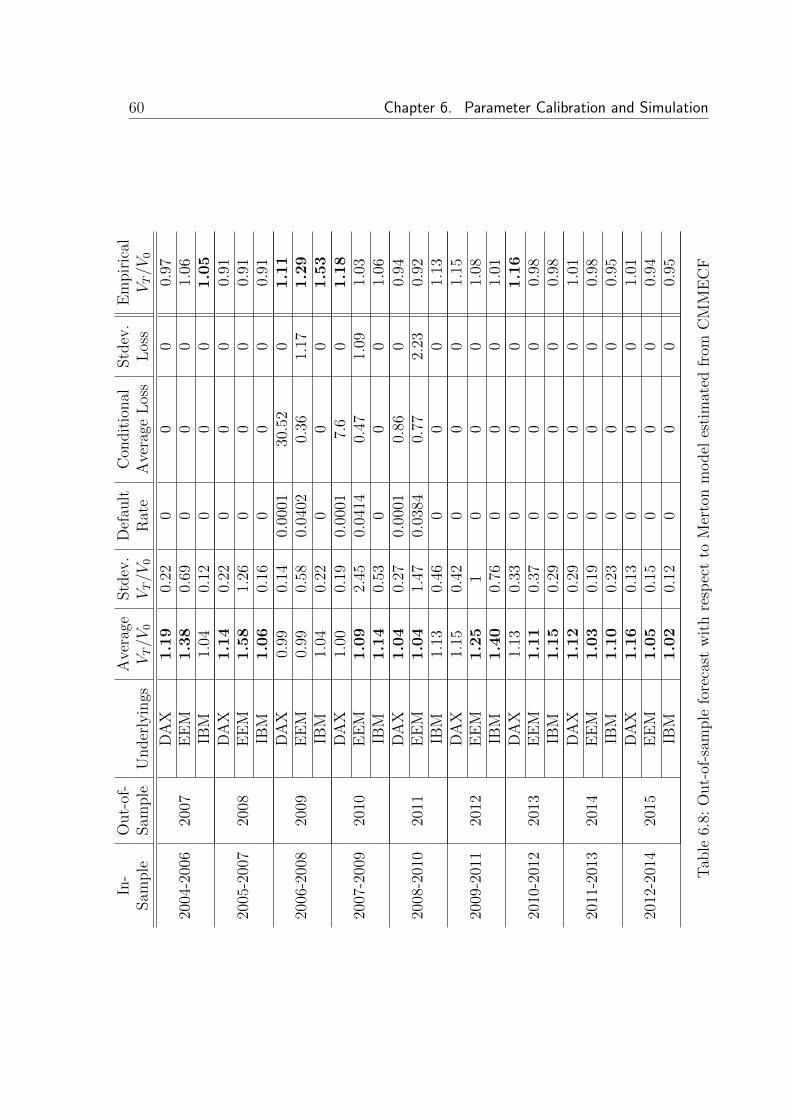
60 Chapter 6. Parameter Calibration and SimulationIn

-O

ut-

of-

Ave

rage

Std

ev.

Def

ault

Con

dit

ional

Std

ev.

Em

pir

ical

Sam

ple

Sam

ple

Under

lyin

gsVT/V

0VT/V

0R

ate

Ave

rage

Los

sL

oss

VT/V

0

2004

-200

620

07D

AX

1.19

0.22

00

00.

97E

EM

1.38

0.69

00

01.

06IB

M1.

040.

120

00

1.05

2005

-200

720

08D

AX

1.14

0.22

00

00.

91E

EM

1.58

1.26

00

00.

91IB

M1.06

0.16

00

00.

91

2006

-200

820

09D

AX

0.99

0.14

0.00

0130

.52

01.11

EE

M0.

990.

580.

0402

0.36

1.17

1.29

IBM

1.04

0.22

00

01.53

2007

-200

920

10D

AX

1.00

0.19

0.00

017.

60

1.18

EE

M1.09

2.45

0.04

140.

471.

091.

03IB

M1.14

0.53

00

01.

06

2008

-201

020

11D

AX

1.04

0.27

0.00

010.

860

0.94

EE

M1.04

1.47

0.03

840.

772.

230.

92IB

M1.

130.

460

00

1.13

2009

-201

120

12D

AX

1.15

0.42

00

01.

15E

EM

1.25

10

00

1.08

IBM

1.40

0.76

00

01.

01

2010

-201

220

13D

AX

1.13

0.33

00

01.16

EE

M1.11

0.37

00

00.

98IB

M1.15

0.29

00

00.

98

2011

-201

320

14D

AX

1.12

0.29

00

01.

01E

EM

1.03

0.19

00

00.

98IB

M1.10

0.23

00

00.

95

2012

-201

420

15D

AX

1.16

0.13

00

01.

01E

EM

1.05

0.15

00

00.

94IB

M1.02

0.12

00

00.

95

Tab

le6.

8:O

ut-

of-s

ample

fore

cast

wit

hre

spec

tto

Mer

ton

model

esti

mat

edfr

omC

MM

EC

F

6.3. Forecasting Ability 61

In-

Out-

of-

Ave

rage

Std

ev.

Def

ault

Con

dit

ional

Std

ev.

Em

pir

ical

Sam

ple

Sam

ple

Under

lyin

gsVT/V

0VT/V

0R

ate

Ave

rage

Los

sL

oss

VT/V

0

2004

-200

620

07D

AX

1.22

0.24

00

00.

97E

EM

1.40

0.68

00

01.

06IB

M1.

050.

130

00

1.05

2005

-200

720

08D

AX

1.17

0.23

00

00.

91E

EM

1.46

1.12

00

00.

91IB

M1.09

0.18

00

00.

91

2006

-200

820

09D

AX

0.99

0.17

00

01.11

EE

M1.

030.

920.

0005

0.29

0.61

1.29

IBM

1.05

0.26

00

01.53

2007

-200

920

10D

AX

1.00

0.21

00

01.18

EE

M1.11

1.41

0.00

010.

050

1.03

IBM

1.14

0.54

00

01.

06

2008

-201

020

11D

AX

1.04

0.34

00

00.

94E

EM

1.10

1.67

00

00.

92IB

M1.14

0.48

00

01.

13

2009

-201

120

12D

AX

1.17

0.48

00

01.

15E

EM

1.26

1.02

00

01.

08IB

M1.40

0.75

00

01.

01

2010

-201

220

13D

AX

1.15

0.36

00

01.16

EE

M1.09

0.33

00

00.

98IB

M1.17

0.29

00

00.

98

2011

-201

320

14D

AX

1.13

0.32

00

01.

01E

EM

1.05

0.22

00

00.

98IB

M1.13

0.26

00

00.

95

2012

-201

420

15D

AX

1.16

0.23

00

01.

01E

EM

1.06

0.16

00

00.

94IB

M1.04

0.14

00

00.

95

Tab

le6.

9:O

ut-

of-s

ample

fore

cast

wit

hre

spec

tto

new

model

esti

mat

edfr

omC

MM

EC

F

7 | Conclusion

The protection from the CPPI strategies is incomplete due to the well-recognized gap risk.For those portfolios whose guarantees are failed to be fulfilled at maturity, the issuers needto compensate the investors for the gap between the guarantee and the final portfolio value,which might further result in violations of regulations, e.g. Solvency II.

In view of above, this work gives contribution to not only the evaluation of the risk measureunder the consideration of gap risk in CPPI portfolios, but also the generalization of theCPPI strategies.

On the perspective of the risky asset dynamic, two well-known models, Merton and Kou,are examined. We observed their insufficiency on capturing the right tail. Therefore, amodification is launched by introducing a Gumbel variable to characterize the size of jumps.From the result of AIC it is shown that this modification outperformed Merton model interms of 5-parameter models.

We generalized the setup of CPPI strategies by loosening the traditional restriction, inwhich the non-risky asset follows the riskfree rate. In the thesis, this restriction is relaxedby allowing the non-risky asset evolving with another yield, which is reasonably assumedto be greater than the riskfree rate. Accordingly, we generalized the CPPI strategy byproviding a bigger pool of possible non-risky investments to select from. For the generalizedself-financing CPPI strategy, a continuous-time stochastic model is constructed. Therein wederived a closed-form solution to the SDE for the cushion dynamic, which can be explicitlywritten as a generalized Ornstein-Uhlenbeck process. The solution for the portfolio valueis obtained according to the mechanics of the insurance strategy after its cushion dynamicbeing solved.

An interesting extension with regard to CPPI strategies is to set the riskfree rate or the yieldto follow another arbitrary Levy process, instead of a constant. Moreover, now that we haveloosed the restriction on the yield of the non-risky asset, how to hedge under the new setupis also another problem that is worth further investigation.

Another focus is set on the problem of the long-term guarantee in the CPPI strategies andhow to describe it mathematically. We provided the statistical evaluation of probability,expectation and variance of loss with the help of the derived closed-form expression. Basedon the existence of the characteristic function we also used the Fourier inversion theorem toretrieve the distribution function in order to derive the VaR and CVaR.

Particular interest is attracted to the numerical performance of the new model setup withrespect to the risky investment and the CPPI portfolio. In addition, the comparison amongthree models are being investigated empirically. We selected various types of risky assets from

64 Chapter 7. Conclusion

global markets, including Asia, Europe and the United States. Parameters are estimatedfrom three methods, each of the three started with two different types of initial values.According to the estimation results, we observed that initial values estimated from CMMmethod not only did not bring out evident effect on behalf of AIC, but also did not improvethe time-efficiency.

In the aspect of estimation methods, we discovered that on one hand, parameters estimatedfrom MLE had the lowest values from AIC, but cost almost one hour in Kou and new models;on the other hand, ECF had the best time-efficiency when estimating, yet the likelihood withrespect to the parameters was relatively small. Nevertheless, the combination of ECF andMLE exhibited remarkable improvements by saving 30-50% of elapsed time, the performanceof the parameters is not a bit compromised by its time-efficiency.

Given that Kou has one more parameter than the other two models, Kou model performedbetter in most of the cases, except for the case when parameters are estimated from theCMMECF. In this very case, the modified new model outperformed the other two. Thus,we provided Q-Q plots for our target underlyings with their parameters estimated fromCMMECF and ECFMLE with respect to each of the three models. From the plots we foundthat right tails of each underlying are better captured in the new model. However, oneshould be cautious while applying the new model, since the improvement on fitting the righttail could have compromised the ability of capturing the left tail.

In this thesis we proposed another weight function for the application in the ECF method.This weight function possesses both the advantages from exponential and normal weightedfunctions, respectively. Since the focus is to assess the risk exposure, assigning more weighton the left tail is worthwhile being further investigated.

We examined the forecasting ability of each model from 2004 to 2014 by taking three yearsas the in-sample period, and the following year as the out-of-sample period. The resultshowed that all three models were in general too optimistic. The Kendall’s τ of each assetbetween simulated and empirical ratios (VT /V0) were very low ([−0.3, 0.2]) with p-Valuesgreater than 0.4. In this manner, we concluded all three models are lack of the ability toforecast. Nevertheless, from the results we observed evidently the downside-risk protectionprovided by the CPPI strategies.

In this thesis we have generalized the CPPI strategies and proposed another dynamic for therisky asset, which can be seen as a start to reexamine and compare other portfolio insurancestrategies based on the similar manner. Especially for those strategies that consist of non-risky investments, e.g. time-invariant portfolio protection strategies, which are variation ofthe CPPI strategies, see [Mantilla-Garcıa, 2014]. Moreover, discrete-time trading as well astrading costs can also be taken into account for further research.

Appendices

65

66

Type Symbol Name

Index ˆDJI Dow Jones Industrial Average 30ˆFCHI CAC 40ˆFTSE FTSE 100

ˆGDAXI DAX 30ˆGSPC S&P 500ˆHSI Hang Seng Index

ˆN225 Nikkei 225ˆTWII TSEC Weighted Index

ETF EEM iShares MSCI Emerging MarketsEZU iShares MSCI Eurozone

Stock AAPL Apple Inc.BA The Boeing CompanyDIS The Walt Disney CompanyGS The Goldman Sachs Group, Inc.HD The Home Depot, Inc.IBM International Business Machines Corporation

MMM 3M CompanyNKE NIKE, Inc.TRV The Travelers Companies, Inc.UNH UnitedHealth Group Incorporated

ALV.DE Allianz SEBAS.DE BASF SE

BAYN.DE Bayer AGBMW.DE Bayerische Motoren Werke AGDAI.DE Daimler AGDBK.DE Deutsche Bank AGDTE.DE Deutsche Telekom AGLIN.DE Linde AGSAP.DE SAP SESIE.DE Siemens AG

Table A.1: Analyzed undelyings from U.S. Dow Jones (July, 2015), German DAX(June, 2015), indices and ETFs

67

Symbol µ σ λ p η+ η− AIC

ˆDJI 0.1515 0.1148 49.9959 0.5466 0.0141 0.0157 -16057.1ˆFTSE 0.2392 0.1288 49.9932 0.6908 0.0167 0.0133 -15717.5

ˆGDAXI 0.3877 0.157 50.0104 0.7546 0.0196 0.0145 -14878.4ˆGSPC 0.2623 0.1251 49.9987 0.6429 0.017 0.0158 -15687ˆHSI 0.4253 0.1729 49.9854 0.8053 0.0276 0.0153 -14369.2

ˆN225 0.1598 0.1783 50.0003 0.4635 0.0134 0.0204 -14280.2ˆTWII 0.4482 0.1525 49.9867 0.8642 0.0175 0.0118 -15341.6ˆFCHI 0.1944 0.1605 50.0035 0.6316 0.0179 0.0166 -14662.6EEM 0.3599 0.2104 49.9943 0.6441 0.0278 0.0242 -13138.7EZU 0.3212 0.1869 50.0195 0.6386 0.0244 0.023 -13747

ALV.DE 0.3207 0.2047 49.871 0.6535 0.0315 0.0247 -13163.5BAS.DE 0.1836 0.2042 50.0033 0.5268 0.0214 0.0211 -13476.2

BAYN.DE 0.26 0.2038 50.0043 0.5413 0.0192 0.0198 -13565.3BMW.DE 0.2402 0.2384 50.0021 0.5905 0.0253 0.0203 -12839.6DAI.DE 0.2806 0.2473 49.9988 0.5818 0.0276 0.0256 -12500.8DBK.DE 0.169 0.25 55.7234 0.6031 0.036 0.0294 -12035.3DTE.DE 0.2492 0.1726 50.0066 0.7327 0.0228 0.0136 -14445.7LIN.DE 0.3453 0.1769 50.0049 0.6629 0.0215 0.0173 -14206.6SAP.DE 0.4452 0.1695 50.0027 0.8046 0.0266 0.0145 -14449.7SIE.DE -0.0068 0.2167 35.3925 0.3506 0.021 0.032 -13392.9

AAPL 0.47 0.2662 49.9925 0.5572 0.025 0.0233 -12334.7BA 0.2921 0.2098 50.0077 0.5896 0.0214 0.0213 -13435.9DIS 0.2569 0.1857 49.9987 0.5918 0.0222 0.0191 -13904.8GS 0.2115 0.2371 49.9977 0.5425 0.029 0.0304 -12429.9HD 0.2029 0.2041 50.0032 0.6195 0.0228 0.0163 -13675.5IBM 0.295 0.155 50.0037 0.6758 0.017 0.0147 -14972.5

MMM 0.3732 0.1539 49.9957 0.692 0.0185 0.016 -14903.6NKE 0.2266 0.179 50.0048 0.5891 0.025 0.0189 -13954.1TRV 0.309 0.1712 49.9782 0.6455 0.0269 0.0196 -14071.2UNH 0.0539 0.2148 49.9909 0.4201 0.0218 0.0279 -13083.5

Table A.2: Parameters of Kou model estimated by ECF using presumed initial values

68


ˆDJI 0.3238 0.1188 49.9888 0.7559 0.0183 0.013 -16039.7ˆFTSE 0.1124 0.113 74.3454 0.52 0.0122 0.0135 -15741.4

ˆGDAXI 0.4478 0.159 50.0997 0.8219 0.023 0.0137 -14873.6ˆGSPC 0.2742 0.1248 50.6269 0.6547 0.0172 0.0156 -15688ˆHSI 0.3161 0.169 49.9795 0.6935 0.0217 0.0171 -14379.9

ˆN225 -0.0229 0.1877 50.0967 0.2342 0.01 0.03 -14261.5ˆTWII 0.2843 0.1507 49.9994 0.6462 0.0117 0.0137 -15347.7ˆFCHI 0.3417 0.1651 49.53 0.7947 0.0237 0.0144 -14660.4EEM 0.3646 0.2106 49.9683 0.648 0.0279 0.0241 -13138.5EZU 0.2857 0.1704 27.3319 0.5176 0.8957 0.6149 -12849.6

ALV.DE 0.3883 0.1875 72.2725 0.6547 0.0263 0.0209 -13182.8BAS.DE 0.1837 0.2042 49.9891 0.5269 0.0214 0.0211 -13476.2

BAYN.DE 0.26 0.2039 49.9911 0.5414 0.0192 0.0198 -13565.3BMW.DE 0.4671 0.2057 121.652 0.656 0.019 0.0139 -12866.7DAI.DE 0.367 0.2467 57.0994 0.637 0.0264 0.0217 -12503.5DBK.DE 0.169 0.25 55.7152 0.6031 0.036 0.0294 -12035.3DTE.DE 0.2072 0.1749 43.8382 0.7041 0.0229 0.0146 -14444.6LIN.DE 0.3453 0.1769 49.9928 0.6629 0.0215 0.0173 -14206.6SAP.DE 0.3573 0.1774 34.8366 0.7824 0.0298 0.0169 -14448.4SIE.DE -0.0851 0.2081 49.8768 0.3123 0.0177 0.0287 -13400.3

AAPL 0.5727 0.2275 133.8625 0.5697 0.0172 0.0156 -12362.3BA 0.8393 0.174 151.244 0.7574 0.0169 0.0117 -13451.2DIS 0.2611 0.1839 52.7572 0.5921 0.0217 0.0187 -13907.3GS 0.2319 0.2515 33.5552 0.5812 0.0385 0.0362 -12410.8HD 0.2225 0.2012 55.85 0.6297 0.022 0.0156 -13682.1IBM 0.3468 0.126 111.8565 0.618 0.0122 0.0115 -15003.1

MMM 0.4185 0.1295 94.1993 0.6385 0.014 0.0132 -14938.5NKE 0.2265 0.179 49.9948 0.5891 0.025 0.0189 -13954.1TRV 0.1927 0.2004 17.3608 0.585 0.0442 0.0353 -13970.8UNH 0.0665 0.2176 46.0218 0.4265 0.0227 0.0289 -13082.1

Table A.3: Parameters of Kou model estimated by ECF using CMM initial values

69


ˆDJI 0.3334 0.0721 196.9474 0.5926 0.0085 0.0083 -16138.5ˆFTSE 0.0012 0.0886 196.4289 0.4307 0.0074 0.0096 -15758.5

ˆGDAXI 0.0091 0.0644 425.5452 0.415 0.0061 0.0082 -14925.3ˆGSPC -0.0029 0.0797 193.6681 0.4071 0.0077 0.011 -15744.9ˆHSI -0.0057 0.047 472.2244 0.437 0.0069 0.0086 -14454.5

ˆN225 0.2693 0.1736 64.0486 0.5667 0.0138 0.0164 -14282.6ˆTWII 0.2505 0.0842 276.7152 0.4721 0.0064 0.0087 -15449.3ˆFCHI 0.3886 0.1291 152.0699 0.637 0.0114 0.0104 -14682.3EEM 0.5878 0.1814 94.2968 0.7029 0.0245 0.0178 -13159.6EZU 0.6291 0.1335 162.5869 0.6665 0.0153 0.0131 -13806.7

ALV.DE 0.3548 0.1586 127.2283 0.6042 0.02 0.0166 -13198.1BAS.DE 0.3607 0.1675 129.8124 0.5847 0.0157 0.0141 -13496.5

BAYN.DE 0.1817 0.1662 137.8326 0.4968 0.0137 0.0138 -13579.2BMW.DE -0.0095 0.1498 282.9089 0.471 0.0117 0.0121 -12881DAI.DE 0.3286 0.1846 192.9819 0.5493 0.0155 0.0146 -12518.1DBK.DE 0.135 0.2122 108.5138 0.5584 0.0254 0.0226 -12054DTE.DE -0.1414 0.1321 163.0684 0.4204 0.0103 0.0116 -14477LIN.DE 0.4087 0.1474 116.7132 0.6281 0.0151 0.0126 -14224.7SAP.DE 0.1308 0.1604 66.5168 0.4733 0.0145 0.0171 -14467.5SIE.DE -0.0008 0.1881 81.692 0.4191 0.0169 0.0203 -13408.5

AAPL 0.0076 0.1767 279.3681 0.4009 0.0116 0.0144 -12371.2BA 0.3177 0.1714 144.0375 0.543 0.0134 0.0137 -13459.9DIS 0.2356 0.1571 108.3727 0.5501 0.0158 0.0144 -13925.5GS 0.2482 0.2053 89.7066 0.552 0.0252 0.0236 -12447.2HD 0.0036 0.1232 260.2979 0.4919 0.0109 0.0104 -13747.4IBM -0.0015 0.1221 135.2217 0.4031 0.0095 0.0127 -15014

MMM 0.0037 0.111 175.2258 0.3821 0.0086 0.0127 -14946NKE 0.3516 0.1449 130.3912 0.6065 0.0162 0.0128 -13976.8TRV 0.1665 0.1401 94.9343 0.5127 0.018 0.0177 -14108.1UNH -0.0011 0.1915 84.0531 0.4573 0.0197 0.0219 -13091.3

Table A.4: Parameters of Kou model estimated by MLE using presumed initial values

70


ˆDJI 0.3333 0.0721 196.8636 0.5926 0.0085 0.0083 -16138.5ˆFTSE 0.1194 0.0906 181.2644 0.4947 0.008 0.0093 -15763

ˆGDAXI 0.323 0.0719 376.269 0.5146 0.007 0.0078 -14934ˆGSPC 0.3813 0.0799 175.7985 0.6028 0.0098 0.0095 -15769.3ˆHSI -0.2046 0.051 462.2152 0.3856 0.0066 0.0092 -14448.3

ˆN225 0.2692 0.1736 64.0384 0.5667 0.0138 0.0164 -14282.6ˆTWII 0.3853 0.1878 70.551 0.9999 0.0001 0.0032 -14999.6ˆFCHI -0.0113 0.1161 212.1964 0.4391 0.0084 0.0107 -14675.5EEM 0.5878 0.1814 94.279 0.7028 0.0245 0.0179 -13159.6EZU 0.6292 0.1335 162.581 0.6665 0.0153 0.0131 -13806.7

ALV.DE 0.3548 0.1586 127.2282 0.6042 0.02 0.0166 -13198.1BAS.DE 0.3604 0.1675 129.9117 0.5846 0.0157 0.0141 -13496.5

BAYN.DE 0.1817 0.1662 137.8418 0.4968 0.0137 0.0138 -13579.2BMW.DE 0.2569 0.149 285.598 0.5374 0.0123 0.0114 -12882.2DAI.DE 0.3286 0.1846 193.0212 0.5493 0.0155 0.0146 -12518.1DBK.DE 0.0013 0.2126 107.2625 0.519 0.0245 0.0235 -12053.3DTE.DE -0.1414 0.1321 163.0685 0.4204 0.0103 0.0116 -14477LIN.DE 0.1908 0.1494 109.0629 0.5227 0.0139 0.014 -14221.7SAP.DE 0.1308 0.1604 66.5168 0.4733 0.0145 0.0171 -14467.5SIE.DE -0.0997 0.1869 85.8004 0.3746 0.0161 0.0209 -13409


MMM 0.203 0.1143 151.2892 0.4772 0.0098 0.0122 -14948.8NKE 0.3516 0.1449 130.3723 0.6065 0.0162 0.0128 -13976.8TRV 0.1665 0.1401 94.932 0.5127 0.018 0.0177 -14108.1UNH 0.2962 0.1881 89.66 0.5787 0.0214 0.0192 -13095.9

Table A.5: Parameters of Kou model estimated by MLE using CMM initial values

71


ˆDJI 0.3334 0.0721 196.9475 0.5926 0.0085 0.0083 -16138.5ˆFTSE 0.2525 0.0919 172.5455 0.5676 0.0088 0.0089 -15764.9

ˆGDAXI 0.4203 0.0688 387.4424 0.5426 0.0071 0.0076 -14934.7ˆGSPC 0.3813 0.0799 175.7961 0.6028 0.0098 0.0095 -15769.3ˆHSI 0.0351 0.0479 462.51 0.4484 0.007 0.0085 -14454.7


ALV.DE 0.3548 0.1586 127.2283 0.6042 0.02 0.0166 -13198.1BAS.DE 0.3606 0.1675 129.8421 0.5847 0.0157 0.0141 -13496.5

BAYN.DE 0.1817 0.1662 137.8383 0.4968 0.0137 0.0138 -13579.2BMW.DE 0.2569 0.149 285.5978 0.5374 0.0123 0.0114 -12882.2DAI.DE 0.3286 0.1846 193.0213 0.5493 0.0155 0.0146 -12518.1DBK.DE 0.135 0.2122 108.5136 0.5584 0.0254 0.0226 -12054DTE.DE -0.1414 0.1321 163.0683 0.4204 0.0103 0.0116 -14477LIN.DE 0.4088 0.1475 116.6847 0.6281 0.0151 0.0126 -14224.7SAP.DE 0.1308 0.1604 66.5168 0.4733 0.0145 0.0171 -14467.5SIE.DE -0.0997 0.1869 85.8005 0.3746 0.0161 0.0209 -13409


MMM 0.2045 0.1144 150.871 0.4775 0.0098 0.0122 -14948.8NKE 0.3515 0.1449 130.342 0.6065 0.0162 0.0128 -13976.8TRV 0.1665 0.1401 94.9341 0.5127 0.018 0.0177 -14108.1UNH 0.294 0.1884 89.1463 0.5781 0.0215 0.0192 -13095.9

Table A.6: Parameters of Kou model estimated by ECF and MLE using presumedinitial values

72


ˆDJI 0.3334 0.0722 196.8558 0.5926 0.0085 0.0083 -16138.5ˆFTSE 0.2524 0.0919 172.437 0.5676 0.0088 0.0089 -15764.9

ˆGDAXI 0.4203 0.0688 387.2564 0.5427 0.0071 0.0076 -14934.7ˆGSPC 0.3812 0.0799 175.8698 0.6027 0.0098 0.0095 -15769.3ˆHSI 0.0438 0.0499 457.778 0.4489 0.007 0.0086 -14454.5


ALV.DE 0.3548 0.1586 127.2284 0.6042 0.02 0.0166 -13198.1BAS.DE 0.3606 0.1675 129.8421 0.5847 0.0157 0.0141 -13496.5

BAYN.DE 0.1817 0.1662 137.8422 0.4968 0.0137 0.0138 -13579.2BMW.DE 0.2569 0.149 285.5979 0.5374 0.0123 0.0114 -12882.2DAI.DE 0.3286 0.1846 192.982 0.5493 0.0155 0.0146 -12518.1DBK.DE 0.135 0.2122 108.5136 0.5584 0.0254 0.0226 -12054DTE.DE -0.1414 0.1321 163.0689 0.4204 0.0103 0.0116 -14477LIN.DE 0.4087 0.1474 116.7129 0.6281 0.0151 0.0126 -14224.7SAP.DE 0.1308 0.1604 66.5168 0.4733 0.0145 0.0171 -14467.5SIE.DE -0.0998 0.1869 85.8207 0.3746 0.0161 0.0209 -13409


MMM 0.2045 0.1144 150.8712 0.4775 0.0098 0.0122 -14948.8NKE 0.3516 0.1449 130.3867 0.6065 0.0162 0.0128 -13976.8TRV 0.1666 0.1401 94.9245 0.5128 0.018 0.0177 -14108.1UNH 0.2939 0.1884 89.118 0.5781 0.0215 0.0193 -13095.9

Table A.7: Parameters of Kou model estimated by ECF and MLE using CMM initialvalues

73

Symbol µ σ λ µj σj AIC

ˆDJI 0.1628 0.0965 49.9778 -0.0024 0.022 -16061.9ˆFTSE 0.1198 0.1091 49.9713 -0.0018 0.0221 -15711.9

ˆGDAXI 0.2325 0.1403 49.9823 -0.0033 0.0236 -14875.5ˆGSPC 0.1861 0.1031 49.9766 -0.0026 0.0243 -15698.8ˆHSI 0.1879 0.1528 49.984 -0.003 0.0267 -14383

ˆN225 0.2545 0.1605 49.9804 -0.0036 0.0253 -14248.6ˆTWII 0.2714 0.1375 49.9711 -0.0044 0.0195 -15402.9ˆFCHI 0.1317 0.1459 49.9842 -0.0028 0.0248 -14651.8EEM 0.2481 0.1934 50.0021 -0.0038 0.0353 -13124.5EZU 0.2594 0.1728 49.9951 -0.005 0.0314 -13767.8

ALV.DE 0.1805 0.1861 50.001 -0.0033 0.0371 -13160.3BAS.DE 0.1637 0.1882 50.0016 -0.0007 0.0306 -13469.8

BAYN.DE 0.2443 0.1887 49.9959 -0.0016 0.0285 -13542.7BMW.DE 0.1416 0.2234 50.0057 -0.0002 0.0323 -12849.4DAI.DE 0.2258 0.2362 50.0102 -0.0026 0.035 -12491.6DBK.DE 0.0379 0.2384 50.0062 -0.0023 0.0451 -12024.2DTE.DE 0.0496 0.1541 49.9927 -0.0005 0.0248 -14445.3LIN.DE 0.2224 0.1592 49.9874 -0.0021 0.0276 -14201.3SAP.DE 0.2069 0.1495 49.9842 -0.0024 0.0257 -14425SIE.DE 0.1022 0.1901 49.9994 0.0004 0.0308 -13371

AAPL 0.4184 0.2523 50.0117 -0.0011 0.0342 -12344.9BA 0.2691 0.1998 50.0005 -0.0035 0.0287 -13448.6DIS 0.177 0.1683 49.9929 -0.001 0.0296 -13905.8GS 0.1751 0.2608 20.031 -0.0067 0.0627 -12386.5HD 0.0746 0.1879 49.9993 0.0005 0.028 -13710.3IBM 0.1919 0.138 49.9715 -0.0024 0.0234 -14997.6

MMM 0.2605 0.1355 49.9846 -0.0032 0.025 -14926.4NKE 0.1207 0.1596 49.996 0.0005 0.0309 -13939.3TRV 0.166 0.1505 49.9922 -0.0011 0.0317 -14060.6UNH 0.1477 0.1976 49.9985 -0.0003 0.0344 -13049.2

Table A.8: Parameters of Merton model estimated by ECF using presumed initialvalues

74


ˆDJI 0.1266 0.136 15.5154 -0.0055 0.032 -15957.4ˆFTSE 0.1 0.1371 22.2441 -0.0031 0.0284 -15683.3

ˆGDAXI 0.1914 0.1683 20.0096 -0.0063 0.0314 -14855.3ˆGSPC 0.1564 0.139 20.684 -0.0051 0.0323 -15618.7ˆHSI 0.1675 0.1716 30.9204 -0.0043 0.0312 -14363.5


ALV.DE 0.1697 0.2031 36.7402 -0.0042 0.042 -13155.9BAS.DE 0.1615 0.232 11.4894 -0.0026 0.0567 -13423.3

BAYN.DE 0.2393 0.1995 37.3982 -0.002 0.0315 -13547.6BMW.DE 0.1428 0.241 30.8547 -0.0003 0.0385 -12837.2DAI.DE 0.2115 0.2568 29.2921 -0.004 0.0431 -12490.2DBK.DE 0.0288 0.2641 30.988 -0.0035 0.0565 -12016.5DTE.DE 0.0453 0.1946 9.5679 -0.0013 0.0461 -14398.5LIN.DE 0.1919 0.203 11.3028 -0.0073 0.0484 -14149.6SAP.DE 0.1778 0.1798 19.5716 -0.0048 0.0354 -14447.2SIE.DE 0.1198 0.2279 15.339 0.0005 0.0499 -13370.1

AAPL 0.4044 0.293 9.3209 -0.0044 0.1747 -12179BA 0.3287 0.147 123.2947 -0.0019 0.0218 -13355.5DIS 0.1707 0.2007 20.4466 -0.0019 0.0414 -13878.1GS 0.1751 0.2608 20.0427 -0.0067 0.0626 -12386.6HD 0.0825 0.2103 25.1404 0.001 0.0356 -13666.3IBM 0.168 0.1613 24.334 -0.0041 0.0293 -14966.8

MMM 0.2604 0.1355 49.922 -0.0032 0.0251 -14926.4NKE 0.1245 0.1737 37.4945 0.0007 0.0343 -13944.8TRV 0.158 0.1929 18.2324 -0.0022 0.0479 -13998.8UNH 0.1538 0.2313 21.3682 -0.001 0.0489 -13057.6

Table A.9: Parameters of Merton model estimated by ECF using CMM initial values

75


ˆDJI 0.204 0.0971 66.6324 -0.0022 0.0189 -16081.5ˆFTSE 0.1752 0.1134 59.3609 -0.0023 0.0197 -15727.4


ˆN225 0.2184 0.1865 23.9427 -0.0066 0.0325 -14273.3ˆTWII 0.3411 0.1201 66.7075 -0.0043 0.0187 -15424ˆFCHI 0.1864 0.1541 46.8014 -0.0036 0.0246 -14657.6EEM 0.2674 0.2 42.6912 -0.004 0.0401 -13129.4EZU 0.2884 0.1622 60.9128 -0.004 0.0298 -13772.2

ALV.DE 0.1369 0.1901 48.1391 -0.001 0.0395 -13163.6BAS.DE 0.235 0.1944 44.9435 -0.0022 0.0327 -13472.3

BAYN.DE 0.2073 0.2027 34.5214 -0.0004 0.0347 -13550.5BMW.DE 0.1415 0.2152 57.5933 0.0002 0.0315 -12850.9DAI.DE 0.2002 0.2435 41.5244 -0.0013 0.0393 -12494.6DBK.DE 0.0139 0.2422 46.5493 -0.0005 0.0493 -12027.4DTE.DE 0.03 0.162 44.9109 0.0003 0.0262 -14448.9LIN.DE 0.2098 0.1696 41.3354 -0.0015 0.0298 -14205.4SAP.DE 0.1754 0.1728 27.8741 -0.0027 0.0327 -14451.4SIE.DE 0.0987 0.2086 31.2722 -0.0001 0.0397 -13384.1

AAPL 0.4442 0.2423 56.1273 -0.0016 0.0342 -12347BA 0.2772 0.1948 51.5347 -0.0028 0.0292 -13450DIS 0.1601 0.1748 45.6433 -0.0002 0.0309 -13907.8GS 0.1673 0.2291 41.1033 -0.0017 0.0492 -12412.2HD 0.0664 0.1717 64.2284 0.001 0.0266 -13719.5IBM 0.1553 0.1391 50.6664 -0.0016 0.0233 -14998.5

MMM 0.2622 0.1369 52.6817 -0.003 0.0242 -14927.5NKE 0.1678 0.1723 44.6095 0.0001 0.032 -13947.2TRV 0.1644 0.1569 45.9636 -0.0005 0.0355 -14066.7UNH 0.1519 0.2164 31.8868 -0.0011 0.0454 -13066.4

Table A.10: Parameters of Merton model estimated by MLE using presumed initialvalues

76


ˆDJI 0.204 0.0971 66.6324 -0.0022 0.0189 -16081.5ˆFTSE 0.1752 0.1134 59.3609 -0.0023 0.0197 -15727.4



ALV.DE 0.1369 0.1901 48.1391 -0.001 0.0395 -13163.6BAS.DE 0.235 0.1944 44.9435 -0.0022 0.0327 -13472.3



MMM 0.2622 0.1369 52.6817 -0.003 0.0242 -14927.5NKE 0.1678 0.1723 44.6095 0.0001 0.032 -13947.2TRV 0.1644 0.1569 45.9636 -0.0005 0.0355 -14066.7UNH 0.1519 0.2164 31.8868 -0.0011 0.0454 -13066.4

Table A.11: Parameters of Merton model estimated by MLE using CMM initial values

77


ˆDJI 0.204 0.0971 66.6323 -0.0022 0.0189 -16081.5ˆFTSE 0.1752 0.1134 59.3609 -0.0023 0.0197 -15727.4



ALV.DE 0.1369 0.1901 48.1391 -0.001 0.0395 -13163.6BAS.DE 0.235 0.1944 44.9435 -0.0022 0.0327 -13472.3



MMM 0.2622 0.1369 52.6818 -0.003 0.0242 -14927.5NKE 0.1678 0.1723 44.6095 0.0001 0.032 -13947.2TRV 0.1644 0.1569 45.9636 -0.0005 0.0355 -14066.7UNH 0.1519 0.2164 31.8868 -0.0011 0.0454 -13066.4

Table A.12: Parameters of Merton model estimated by ECF and MLE using presumedinitial values

78


ˆDJI 0.204 0.0971 66.6324 -0.0022 0.0189 -16081.5ˆFTSE 0.1752 0.1134 59.3609 -0.0023 0.0197 -15727.4



ALV.DE 0.1369 0.1901 48.1391 -0.001 0.0395 -13163.6BAS.DE 0.235 0.1944 44.9435 -0.0022 0.0327 -13472.3



MMM 0.2622 0.1369 52.6817 -0.003 0.0242 -14927.5NKE 0.1678 0.1723 44.6095 0.0001 0.032 -13947.2TRV 0.1644 0.1569 45.9636 -0.0005 0.0355 -14066.7UNH 0.1519 0.2164 31.8868 -0.0011 0.0454 -13066.4

Table A.13: Parameters of Merton model estimated by ECF and MLE using CMMinitial values

79

Symbol µ σ λ α β AIC

ˆDJI 0.3924 0.0961 49.9453 -0.0162 0.0168 -16046.4ˆFTSE 0.3513 0.1102 49.9516 -0.0156 0.0167 -15714.7


ˆN225 0.4898 0.1593 49.9738 -0.0188 0.0194 -14236.3ˆTWII 0.4923 0.1338 49.9489 -0.017 0.0146 -15412.9ˆFCHI 0.3672 0.1449 49.9679 -0.0179 0.0191 -14666.1EEM 0.4765 0.1923 49.9977 -0.0225 0.0284 -13136EZU 0.49 0.1698 49.9888 -0.0224 0.0249 -13766

ALV.DE 0.4028 0.1853 49.9925 -0.0224 0.0302 -13158.9BAS.DE 0.3996 0.1909 49.9884 -0.0179 0.0242 -13480

BAYN.DE 0.4849 0.1903 49.9862 -0.0181 0.0223 -13550.3BMW.DE 0.3805 0.2258 49.998 -0.0182 0.0257 -12847DAI.DE 0.4642 0.2363 50.0007 -0.0215 0.0281 -12498DBK.DE 0.1174 0.2697 26.8069 -0.029 0.0524 -12003.3DTE.DE 0.2845 0.1567 49.9733 -0.0155 0.0192 -14441.5LIN.DE 0.4596 0.16 49.9777 -0.0182 0.0216 -14199.4SAP.DE 0.4427 0.1491 49.9685 -0.0179 0.02 -14408.5SIE.DE 0.3364 0.1946 49.9909 -0.0167 0.0242 -13351.5

AAPL 0.664 0.2541 50.0159 -0.0199 0.0272 -12333.8BA 0.5091 0.1985 50.0005 -0.0202 0.0225 -13451.1DIS 0.4117 0.1706 49.9871 -0.0178 0.0233 -13898.5GS 0.2112 0.2669 15.9436 -0.0349 0.0627 -12368.5HD 0.3109 0.1914 49.9902 -0.0158 0.022 -13703.4IBM 0.4278 0.1382 49.9565 -0.0169 0.0178 -14965.2

MMM 0.496 0.1344 49.9612 -0.0183 0.0193 -14902.7NKE 0.349 0.1637 49.9861 -0.0167 0.0246 -13952.4TRV 0.3952 0.1525 49.9847 -0.0185 0.0254 -14058.8UNH 0.3808 0.201 49.9958 -0.0187 0.0274 -13049.7

Table A.14: Parameters of new model estimated by ECF using presumed initial values

80


ˆDJI 0.382 0.0981 47.7773 -0.0164 0.017 -16047.8ˆFTSE 0.3506 0.1103 49.8413 -0.0156 0.0168 -15714.8


ˆN225 0.4927 0.1596 49.9642 -0.0188 0.0193 -14237.1ˆTWII 0.8298 0.095 116.0681 -0.0132 0.0114 -15363.5ˆFCHI 0.3621 0.1456 49.0643 -0.0179 0.0193 -14666.6EEM 0.4719 0.1931 49.2803 -0.0226 0.0286 -13136EZU 0.482 0.1711 48.7862 -0.0225 0.0251 -13765.2

ALV.DE 0.4028 0.1853 49.9859 -0.0225 0.0302 -13158.9BAS.DE 0.3993 0.1909 49.935 -0.0179 0.0242 -13479.9

BAYN.DE 0.4848 0.1903 49.978 -0.0181 0.0223 -13550.3BMW.DE 0.3802 0.2258 49.9502 -0.0182 0.0257 -12847DAI.DE 0.4639 0.2364 49.9467 -0.0215 0.0281 -12498DBK.DE 0.1173 0.2697 26.7917 -0.029 0.0524 -12003.2DTE.DE 0.2836 0.1569 49.7985 -0.0155 0.0192 -14441.6LIN.DE 0.4585 0.1602 49.792 -0.0182 0.0216 -14199.4SAP.DE 0.4415 0.1492 49.753 -0.0179 0.02 -14408.9SIE.DE 0.332 0.1954 49.0939 -0.0168 0.0244 -13351.8

AAPL 0.6639 0.2541 50.0027 -0.0199 0.0272 -12333.8BA 0.4989 0.1998 48.3685 -0.0203 0.0228 -13451.2DIS 0.4078 0.1713 49.2536 -0.0178 0.0234 -13898.6GS 0.2112 0.2669 15.9421 -0.0349 0.0627 -12368.5HD 0.3109 0.1914 49.9932 -0.0158 0.022 -13703.4IBM 0.4276 0.1382 49.9331 -0.0169 0.0178 -14965.2

MMM 0.4965 0.1345 49.927 -0.0184 0.0192 -14902.6NKE 0.3458 0.1644 49.3104 -0.0167 0.0248 -13952.4TRV 0.391 0.1534 49.2116 -0.0186 0.0255 -14059.1UNH 0.3707 0.2028 48.074 -0.0189 0.0278 -13049.8

Table A.15: Parameters of new model estimated by ECF using CMM initial values

81


ˆDJI 0.3534 0.0874 96.5037 -0.0103 0.0128 -16093.3ˆFTSE 0.3228 0.1068 78.5033 -0.0115 0.0138 -15736.2



ALV.DE 0.2808 0.1881 52.4162 -0.0211 0.0312 -13163.4BAS.DE 0.4349 0.1864 58.0473 -0.0184 0.0231 -13481.9

BAYN.DE 0.3826 0.1944 47.695 -0.0177 0.0242 -13552.9BMW.DE 0.5149 0.1881 111.4163 -0.0144 0.0195 -12859DAI.DE 0.4869 0.2274 63.6776 -0.0204 0.0263 -12499.2DBK.DE 0.2057 0.2361 54.2855 -0.0251 0.0376 -12023.3DTE.DE 0.1842 0.1583 54.5025 -0.0136 0.0195 -14446.3LIN.DE 0.4195 0.1562 65.7207 -0.0152 0.0194 -14204.1SAP.DE 0.243 0.1769 22.8471 -0.0224 0.0291 -14443.3SIE.DE 0.2057 0.2129 27.7015 -0.0231 0.0349 -13363

AAPL 0.7842 0.2274 82.6479 -0.0186 0.0235 -12341.9BA 0.4308 0.1981 46.7593 -0.0202 0.0244 -13452.7DIS 0.3205 0.1691 56.5238 -0.0159 0.023 -13901.8GS 0.3399 0.2219 50.0576 -0.0251 0.036 -12408HD 0.3666 0.1509 116.3077 -0.0117 0.0169 -13730.6IBM 0.2539 0.1433 43.7311 -0.0155 0.0205 -14977.2

MMM 0.3591 0.1405 47.0574 -0.017 0.0208 -14911.9NKE 0.3459 0.1613 63.0072 -0.0154 0.0222 -13956.2TRV 0.2712 0.1545 51.1499 -0.0179 0.0275 -14065.7UNH 0.2951 0.2104 38.6419 -0.0236 0.0339 -13057.4

Table A.16: Parameters of new model estimated by MLE using presumed initial values

82


ˆDJI 0.2347 0.0924 80.2538 -0.0107 0.0141 -16086.8ˆFTSE 0.3228 0.1068 78.5032 -0.0115 0.0138 -15736.2



ALV.DE 0.2807 0.1881 52.4003 -0.0211 0.0312 -13163.4BAS.DE 0.4349 0.1864 58.0473 -0.0184 0.0231 -13481.9

BAYN.DE 0.3826 0.1944 47.6759 -0.0177 0.0242 -13552.9BMW.DE 0.5149 0.1881 111.4069 -0.0144 0.0195 -12859DAI.DE 0.4872 0.2274 63.7636 -0.0204 0.0263 -12499.2DBK.DE 0.2057 0.2361 54.2855 -0.0251 0.0376 -12023.3DTE.DE 0.1842 0.1583 54.5026 -0.0136 0.0195 -14446.3LIN.DE 0.4195 0.1562 65.7203 -0.0152 0.0194 -14204.1SAP.DE 0.243 0.1769 22.8471 -0.0224 0.0291 -14443.3SIE.DE 0.2452 0.2126 28.1962 -0.0233 0.0345 -13362.7


MMM 0.3591 0.1405 47.0574 -0.017 0.0208 -14911.9NKE 0.3459 0.1613 63.0072 -0.0154 0.0222 -13956.2TRV 0.2712 0.1545 51.1501 -0.0179 0.0275 -14065.7UNH 0.2951 0.2104 38.642 -0.0236 0.0339 -13057.4

Table A.17: Parameters of new model estimated by MLE using CMM initial values

83


ˆDJI 0.3535 0.0874 96.4994 -0.0103 0.0128 -16093.3ˆFTSE 0.3228 0.1068 78.5032 -0.0115 0.0138 -15736.2



ALV.DE 0.2807 0.1881 52.4003 -0.0211 0.0312 -13163.4BAS.DE 0.4349 0.1864 58.0473 -0.0184 0.0231 -13481.9



MMM 0.3591 0.1405 47.0574 -0.017 0.0208 -14911.9NKE 0.3459 0.1613 63.0071 -0.0154 0.0222 -13956.2TRV 0.2712 0.1545 51.15 -0.0179 0.0275 -14065.7UNH 0.2951 0.2104 38.6419 -0.0236 0.0339 -13057.4

Table A.18: Parameters of new model estimated by ECF and MLE using presumedinitial values

84


ˆDJI 0.3535 0.0874 96.5662 -0.0103 0.0127 -16093.3ˆFTSE 0.3228 0.1068 78.5032 -0.0115 0.0138 -15736.2



ALV.DE 0.2807 0.1881 52.4003 -0.0211 0.0312 -13163.4BAS.DE 0.4349 0.1864 58.0597 -0.0184 0.0231 -13481.9



MMM 0.3591 0.1405 47.0574 -0.017 0.0208 -14911.9NKE 0.3459 0.1613 63.0071 -0.0154 0.0222 -13956.2TRV 0.2712 0.1545 51.15 -0.0179 0.0275 -14065.7UNH 0.2951 0.2104 38.6419 -0.0236 0.0339 -13057.4

Table A.19: Parameters of new model estimated by ECF and MLE using CMM initialvalues

List of Figures

4.1 CPPI on stock price simulated from Black-Scholes model . . . . . . . . . . . 174.2 The effect of jumps on asset price . . . . . . . . . . . . . . . . . . . . . . . . . 184.3 Comparison between different jumps in different distributions with same mean

and variance . . . . . . . . . . . . . . . . . . . . . . . . . . . . . . . . . . . . . 20

5.1 Floor not violated: Different stock dynamics (left: up; right: fluctuate) andthe performance of CPPI strategy . . . . . . . . . . . . . . . . . . . . . . . . 27

5.2 Floor violated: Dynamics of portfolio value (left) and cushion value when thefloor is broken . . . . . . . . . . . . . . . . . . . . . . . . . . . . . . . . . . . . 28

5.3 Floor violated: Dynamics of portfolio value (left) and cushion value when thefloor is broken . . . . . . . . . . . . . . . . . . . . . . . . . . . . . . . . . . . . 29

6.1 Q-Q plots of DAX, iShares MSCI Emerging Markets and IBM empirical quan-tiles versus theoretical quantiles from a normal distribution . . . . . . . . . . 53

6.2 Q-Q plots of DAX empirical quantiles versus theoretical quantiles from eachmodel whose parameters estimated from CMMECF(left) and ECFMLE, re-spectively . . . . . . . . . . . . . . . . . . . . . . . . . . . . . . . . . . . . . . 54

6.3 Q-Q plots of iShares MSCI Emerging Markets empirical quantiles versus the-oretical quantiles from each model whose parameters estimated from CM-MECF(left) and ECFMLE, respectively . . . . . . . . . . . . . . . . . . . . . 55

6.4 Q-Q plots of IBM empirical quantiles versus theoretical quantiles from eachmodel whose parameters estimated from CMMECF(left) and ECFMLE, re-spectively . . . . . . . . . . . . . . . . . . . . . . . . . . . . . . . . . . . . . . 56

85

List of Tables

4.1 Quadratic covariation for time, Brownian motion, and counting process . . . 22

6.1 Parameters-estimating methods and initial values applied in different models 49

6.2 Average AIC and elapsed time (in seconds) with respect to different models . 50

6.3 Average AIC and elapsed time (in seconds) for indices only with respect todifferent models . . . . . . . . . . . . . . . . . . . . . . . . . . . . . . . . . . . 50

6.4 Average AIC and elapsed time (in seconds) for stocks only with respect todifferent models . . . . . . . . . . . . . . . . . . . . . . . . . . . . . . . . . . . 51

6.5 Parameter with respect to target underlyings estimated from CMMECF andECFMLE . . . . . . . . . . . . . . . . . . . . . . . . . . . . . . . . . . . . . . 52

6.6 Simulation results with respect to target underlyings estimated from CM-MECF and ECFMLE . . . . . . . . . . . . . . . . . . . . . . . . . . . . . . . 57

6.7 Out-of-sample forecast with respect to Kou model estimated from CMMECF 59

6.8 Out-of-sample forecast with respect to Merton model estimated from CMMECF 60

6.9 Out-of-sample forecast with respect to new model estimated from CMMECF 61

A.1 Analyzed undelyings from U.S. Dow Jones (July, 2015), German DAX (June,2015), indices and ETFs . . . . . . . . . . . . . . . . . . . . . . . . . . . . . . 66

A.2 Parameters of Kou model estimated by ECF using presumed initial values . . 67

A.3 Parameters of Kou model estimated by ECF using CMM initial values . . . . 68

A.4 Parameters of Kou model estimated by MLE using presumed initial values . . 69

A.5 Parameters of Kou model estimated by MLE using CMM initial values . . . . 70

A.6 Parameters of Kou model estimated by ECF and MLE using presumed initialvalues . . . . . . . . . . . . . . . . . . . . . . . . . . . . . . . . . . . . . . . . 71

A.7 Parameters of Kou model estimated by ECF and MLE using CMM initial values 72

A.8 Parameters of Merton model estimated by ECF using presumed initial values 73

A.9 Parameters of Merton model estimated by ECF using CMM initial values . . 74

A.10 Parameters of Merton model estimated by MLE using presumed initial values 75

A.11 Parameters of Merton model estimated by MLE using CMM initial values . . 76

A.12 Parameters of Merton model estimated by ECF and MLE using presumedinitial values . . . . . . . . . . . . . . . . . . . . . . . . . . . . . . . . . . . . 77

A.13 Parameters of Merton model estimated by ECF and MLE using CMM initialvalues . . . . . . . . . . . . . . . . . . . . . . . . . . . . . . . . . . . . . . . . 78

A.14 Parameters of new model estimated by ECF using presumed initial values . . 79

A.15 Parameters of new model estimated by ECF using CMM initial values . . . . 80

A.16 Parameters of new model estimated by MLE using presumed initial values . . 81

87

88 List of Tables

A.17 Parameters of new model estimated by MLE using CMM initial values . . . . 82A.18 Parameters of new model estimated by ECF and MLE using presumed initial

values . . . . . . . . . . . . . . . . . . . . . . . . . . . . . . . . . . . . . . . . 83A.19 Parameters of new model estimated by ECF and MLE using CMM initial values 84

List of Notation

Abbreviation

CPPI: constant proportion portfolio insurance.

OBPI: option based portfolio insurance.

CPDO: constant proportion debt obligation.

cadlag: right continuous, with left limits.

VaR: value at risk.

CVaR: conditional value at risk.

CMM: cumulant matching method.

MLE: maximum likelihood method.

ECF: empirical characteristic function method.

AIC: Akaike information criterion.

Preliminaries

(Ω,F ,P): probability space.

Ftt≥0: filtration, which is an increasing sequence of σ-algebras withFt ∈ F , ∀t ≥ 0.

τ : stopping time.

∧: infix operator which outputs the minimum of two real scalararguments.

E(X): Doleans-Dade exponential of a semimartingale X.

[X1, X2]: quadratic covariation of two semimartingales X1 and X2.

Jtt≥0: sequence of i.i.d. random variable which generates the jumpsize.

Ntt≥0: counting process.

Ytt≥0: compound Poisson process which is constructed by N and J .

(µR, σ2, ν): Levy R-triplet.

ψZ : cumulant generating function of a random variable Z.

89

90

ci(Z): i-th cumulant of a random variable Z.

CPPI strategy

G: guarantee.

m: multiplier, which offers leverage.

r: riskfree rate.

T : maturity.

y: yield from non-risky asset.

σ: volatility.

Bt: non-risky asset price at time t.

Ct: cushion value at time t.

Pt: discounted guarantee at time t, which forms the floor.

St: risky asset price at time t.

Vt: portfolio value at time t.

Wt: Brownian motion at time t.

αt: the amount of risky investment at time t.

Risk measure

E[X|A]: condtional expectation of X given A.

VaRα: value at risk of the portfolio at the confidence level α.

CVaRα: conditional value at risk of the portfolio at the confidence levelα.

sgn: sign function.

R: operator which acquires the real part from a complex number

Bibliography

Applebaum, D. Levy processes and stochastic calculus. Cambridge University Press, 2009.

Balder, S., Brandl, M., and Mahayni, A. Effectiveness of CPPI strategies under discrete-timetrading. Journal of Economic Dynamics and Control, 33:204–220, 2009.

Bertrand, P. and Prigent, J. L. Portfolio insurance strategies: OBPI versus CPPI. Finance,26:5–32, 2005.

Bertrand, P. and Prigent, J. L. Omega performance measure and portfolio insurance. Journalof Banking and Finance, 35:1811–1823, 2011.

Black, F. and Jones, R. Simplifying portfolio insurance. The Journal of Portfolio Manage-ment, 14:48–51, 1987.

Black, F. and Perold, A. Theory of constant proportion portfolio insurance. The Journal ofEconomic Dynamics and Control, 16:403–426, 1992.

Black, F. and Scholes, M. The pricing of options and corporate liabilities. Journal of PoliticalEconomy, 81:637–659, 1973.

Borak, S., Misiorek, A., and Weron, R. Models for heavy-tailed asset returns. Wroc lawUniversity of Technology, 2010. URL https://mpra.ub.uni-muenchen.de/25494/.

Cai, N. and Kou, S. G. Option pricing under a mixed-exponential jump diffusion model.Management Science, 57:2067–2081, 2011.

Carrasco, M. and Florens, J. P. Generalization of GMM to a continuum of moment condi-tions. Econometric Theory, 16:797–834, 2000.

Chacko, G. and Viceira, L. M. Spectral GMM estimation of continuous-time processes.Journal of Econometrics, 116:259–292, 2003.

Cont, R. and Jessen, C. Constant proportion debt obligations (CPDO): Modeling and riskanalysis. Quantitative Finance, 12:1199–1218, 2012.

Cont, R. and Tankov, P. Financial modelling with jump processes. Financial Mathematics.Chapman and Hall/CRC, 1st edition, 2004.

Cont, R. and Tankov, P. Constant proportion portfolio insurance in presence of jumps inasset prices. Mathematical Finance, 19(3):379–401, 2009.

91

https://mpra.ub.uni-muenchen.de/25494/

92 Bibliography

Devolder, P. Revised version of: Solvency requirement for long term guarantee: risk measureversus probability of ruin. European Actuarial Journal, 1:199–214, 2011.

Eberlein, E. Jump-type Levy processes. In Andersen, T., Davis, R., Kreiß, J.-P., andMikosch, T., editors, Handbook of Financial Time Series, pages 439–455. Springer, 2009.

ECB. Key ECB interest rates. European Central Bank, 2015. URL https://www.ecb.

europa.eu/stats/monetary/rates/html/index.en.html.

Escobar, M., Kiechle, A., Seco, L., and Zagst, R. Option on a CPPI. International Mathe-matical Forum, 6:229–262, 2011.

Etheridge, A. A course in financial calculus. Cambridge University Press, 1st edition, 2002.

Feuerverger, A. An efficiency result for the empirical characteristic function in stationarytime-series models. The Canadian Journal of Statistics, 18:155–161, 1990.

Feuerverger, A. and McDunnough, P. On the Efficiency of Empirical Characteristic FunctionProcedures. Journal of The Royal Statistical Society, 43:20–27, 1981.

Feuerverger, A. and Mureika, R. The empirical characteristic function and its applications.The Annals of Statistics, 5:88–97, 1977.

Gil-Pelaez, J. Note on the inversion theorem. Biometrika, 38(3-4):481–482, 1951.

Gurland, J. Inversion formulae for the distribution of ratios. Annals of Mathematical Statis-tics, 19(2):228–237, 1948.

Gut, A. Probability: a graduate course. Springer, 2005.

Heathcote, C. R. The integrated squared error estimation of parameters. Biometrika, 64:255–264, 1977.

Jiang, G. J. and Knight, J. L. Estimation of continuous-time processes via the empiricalcharacteristic function. Journal of Business and Economic Statistics, 20:198–212, 2002.

Joossens, E. and Schoutens, W. An Overview of Portfolio Insurances: CPPI and CPDO.JRC Scientific and Technical Research Reports, 2008.

Keating, C. and Shadwick, W. F. A universal performance measure. Journal of PerformanceMeasurement, 6:59–84, 2002.

Kou, S. G. A Jump-Diffusion Model for Option Pricing. Management Science, 48:1086–1101,2002.

Kou, S. G. and Wang, H. Option pricing under a double exponential jump diffusion model.Management Science, 50:1178–1192, 2004.

Levin, A. and Khramtsov, V. Estimation of affine jump-diffusions using realized varianceand bipower variation in empirical characteristic function method. Working Paper, RoyalBank of Canada, 2015. URL http://ssrn.com/abstract=2389046.

https://www.ecb.europa.eu/stats/monetary/rates/html/index.en.html

https://www.ecb.europa.eu/stats/monetary/rates/html/index.en.html

http://ssrn.com/abstract=2389046

Bibliography 93

Levy, P. Calcul des Probabilites. Gauthier-Villars, Paris, 1925.

Lin, J. and Shyu, D. CPPI and TIPP Strategies: A Comparison. In Conference on behavioralfinance and emerging market, 2008.

Maller, R. A., Muller, G., and Szimayer, A. Ornstein-Uhlenbeck processes and extensions.In Andersen, T., Davis, R., Kreiß, J.-P., and Mikosch, T., editors, Handbook of FinancialTime Series, pages 421–437. Springer, 2009.

Mantilla-Garcıa, D. Dynamic allocation strategies for absolute and relative loss control.Algorithmic Finance, 3:209–231, 2014.

Merton, R. C. Option pricing when underlying stock returns are discontinuous. Journal ofFinancial Economics, 3:125–144, 1976.

Parzen, E. On estimation of a probability density function and mode. The Annals ofMathematical Statistics, 33:1065–1076, 1962.

Pascucci, A. PDE and martingale methods in option pricing. Springer, 2011.

Paulson, A. S., Holcomb, E. W., and Leitch, R. A. The estimation of the parameters of thestable laws. Biometrika, 62:163–170, 1975.

Perold, A. and Sharpe, W. Dynamic strategies for asset allocation. Financial AnalystJournal, January-February:16–27, 1988.

Pezier, J. and Scheller, J. Best portfolio insurance for long-term investment strategies inrealistic conditions. Insurance: Mathematics and Economics, 52:263–274, 2013.

Polyanin, A. D. and Manzhirov, A. V. Handbook of integral equations. CRC Press, 1998.

Prigent, J. L. and Tahar, F. CPPI with cushion insurance. Working Paper, THEMAUniversity of Cergy-Pontoise, 2005. URL http://ssrn.com/abstract=675824.

Protter, P. E. Stochastic integration and differential equations. Springer, 2nd edition, 2005.

Ramezani, C. A. and Zeng, Y. Maximum likelihood estimation of asymmetric jump-diffusionprocess: Application to security prices. Working Paper, Department of Mathematics andStatistics, Univeristy of Missouri, Kansas City, 1998.

Ramponi, A. VaR-optimal risk management in regime-switching jump-diffusion models.Journal of Mathematical Finance, 3:103–109, 2013.

Rockinger, M. and Semenova, M. Estimation of jump-diffusion processes via empiricalcharacteristic functions. Research Paper, Universite de Geneve, 2005. URL http:

//ssrn.com/abstract=770785.

Sato, K. Levy processes and infinitely divisible distributions. Cambridge University Press,2005.

Weng, C. Constant proportion portfolio insurance under a regime switching exponentialLevy process. Insurance: Mathematics and Economics, 52:508–521, 2013.




94 Bibliography

Weng, C. Discrete-time CPPI under transaction cost and regime switching. Working Paper,Department of Statistics and Actuarial Science, University of Waterloo, 2014. URL http:

//ssrn.com/abstract=2432233.

Yu, J. Empirical characteristic function estimation and its applications. Econometric Re-views, 23:93–123, 2004.



Eidesstattliche Erklarung

Ich erklare hiermit, dass ich diese Dissertation selbststandig und nur unter Zuhilfenahme derangegebenen Hilfsmittel und Quellen angefertigt habe.

Yi-Ting TsaiOldenburg, den 01. Februar 2016

95

Curriculum Vitae

Personal Details

Name Yi-Ting Tsai

Date of birth 09. July 1984

Place of birth Chiayi, Taiwan

Professional Experience

Since Dec. 2012 Carl von Ossietzky University of Oldenburg, GermanyResearch fellow at the institute for mathematics

Aug. 2015–Aug. 2015 Fraunhofer ITWM, GermanyIntern at the department of financial mathematics

Mar. 2011–Oct. 2012 Jihsun Financial Holdings, TaiwanDerivatives trader

Jul. 2010–Aug. 2010 Carl von Ossietzky University of Oldenburg, GermanyIntern at the institute for mathematics, financed by a DAADscholarship

Sep. 2007–Jun. 2010 National Chengchi University, TaiwanM.Sc., Mathematical SciencesTopic of master’s thesis: Portfolio optimization under CVaRcontrol and tracking error minimization

Sep. 2002–Jun. 2006 National Taichung University, TaiwanB.Ed., Mathematics Education

97

Lebenslauf

Personliche Angaben

Name Yi-Ting Tsai

Geburtsdatum 09. Juli 1984

Geburtsort Chiayi, Taiwan

Werdegang

Seit Dez. 2012 Carl von Ossietzky Universitat OldenburgWissenschaftliche Mitarbeiterin am Institut fur Mathematik

Aug. 2015–Aug. 2015 Fraunhofer ITWMPraktikantin an der Abteilung Finanzmathematik

Mar. 2011–Okt. 2012 Jihsun Financial Holdings, TaiwanDerivatehandlerin

Jul. 2010–Aug. 2010 Carl von Ossietzky Universitat OldenburgPraktikantin am Institut fur Mathematik, finanziert durch einDAAD-Stipendium

Sep. 2007–Jun. 2010 National Chengchi University, TaiwanM.Sc., Mathematical SciencesThema der Masterarbeit: Portfolio optimization under CVaRcontrol and tracking error minimization

Sep. 2002–Jun. 2006 National Taichung University, TaiwanB.Ed., Mathematics Education

99

CPPI strategies and the problem of long-term guaranteesoops.uni-oldenburg.de/2743/1/tsacpp16.pdf ·...

Documents

Transcript of CPPI strategies and the problem of long-term guaranteesoops.uni-oldenburg.de/2743/1/tsacpp16.pdf ·...