© Cenit Online 2015

Investment Appraisal

Introduction to Investment Appraisal

Whatever level of management authorises a capital expenditure, the proposed investment should

be properly evaluated, and found to be worthwhile before the decision is taken to go ahead with

the expenditure.

Capital expenditure differs from day to day revenue expenditure as it will involve a bigger outlay

of money. The benefits will also accrue over a much longer period of time and therefore the

benefits cannot all be set against costs in the current year’s profit and loss account.

The identification of an investment opportunity is the most difficult part of the capital investment

process. There are often two or more ways of achieving an objective, and once the different

investment opportunities are identified, they should then be compared.

Acquiring the relevant data to form the basis for an informed decision is one of the most important

aspects in practice. Large capital investments that turn out to be unprofitable can usually be

abandoned only at a substantial loss, therefore time and effort spent in market research and

acquiring data about relevant costs and benefits is rarely wasted. This activity helps to focus

manager’s minds on the reality of the projections as they are forecasting and so weed out poor

projects at an early stage, before they are subjected to intensive financial scrutiny.

Relevant and Non Relevant Costs

A distinction must be made between relevant and non-relevant costs and revenues for the purposes of management decision making.

Relevant costs and revenues are those that CHANGE as a direct result of a decision taken.

- They are future costs and revenues � as it is not possible to change what has happened in the past relevant costs and revenues must be future costs and revenues.

- They are incremental � it is the increase or decrease in costs and revenues that is relevant. - They are cash flows� future costs and revenues must be cash flows arising as a direct

consequence of the decision taken.

Non – relevant costs include:

Sunk Costs:

Money already spent that cannot now be recovered. An example of a sunk cost is expenditure that has been incurred in developing a new product. The money cannot be recovered even if a decision is taken to abandon any further development of the product. The cost therefore is not relevant to future decisions concerning the product.

Committed Costs:

Expenditure that will be incurred in the future, but as a result of decisions taken in the past that cannot now be changed. A committed cost will be incurred regardless of the decision taken and therefore it is not relevant. An example would be expenditure on special packaging for a new product, where the packaging has been ordered and delivered but not yet paid for. The company

is obliged to pay for the packaging even if they decide not to proceed with the product; therefore it is not a relevant cost.

Opportunity Costs:

A special type of relevant cost. The value of the benefit sacrificed when one course of action is chosen over another. The opportunity cost is the foregone potential benefit from the best rejected course of action.

Depreciation:

Depreciation calculations do not result in any future cash flows. They are merely the book entries that are designed to spread the original cost of an asset over its useful life.

Notional Costs:

Notional costs such as notional rent and notional interest are only relevant if they represent an

identified lost opportunity to use a premises or finance for some alternative purpose for example.

In these circumstances the notional costs would be opportunity costs.

Payback Period Payback is the time required for cash inflows from a capital investment project to equal cash

outflows. “How long will it take to payback the cost?” Payback is commonly used as a first

screening method and if a project passes the payback test, it should then be evaluated using

another investment appraisal technique.

Example: Company ABC ltd is considering an investment of €100,000. The desired payback period is 3 years. The board of directors have identified two alternatives; project A and project B. The expected annual cash flows are as follows:

Cash flow:

Y0 Initial Cost:

Project A

(100,000)

Project B

(100,000)

Y1 Cash flow: 35,000 35,000 Y2 Cash flow: 28,000 35,000 Y3 Cash flow: 32,000 35,000 Y4 Cash flow: 40,000 35,000

Required: Calculate the Payback period of each project and advise ABC’s board of directors which project they should invest in.

Solution: Project A: 35,000 + 28,000 + 32,000 = 95,000. In 3 years the company will recover €95,000 of the initial €100,000 outlay.

In year 4 it will recover 40,000. To calculate the fraction of a year remaining � 5,000 / 40,000 = .125 of a year. Thus the payback period is 3.125 years.

Project B: 35,000 + 35,000 + 35,000 = 105,000. In 3 years the company will recover €105,000 of the initial outlay.

In year 3 it will recover 35,000. To calculate the fraction of the year within which the payback period was achieved � 30,000 / 35,000 = .86. Thus the payback period is 2.86 years.

The board of directors of ABC should select project B.

Advantages: Disadvantages:

Quick and easy - ignores time value of money

Used when future cash flow are uncertain - Ignores cash flows beyond payback period

Long term investment is more uncertain - Ignores the risk of future cash flows

Return on Capital Employed The Return on Capital Employed (ROCE) also known as the Accounting Rate of Return (ARR)

estimates the rate of return or the Return on Investment that a project should yield. If it exceeds

a target rate of return then the project will be undertaken.

Where estimated average investment is calculated as (Capital Cost + Disposal Value) / 2

Example:

A company has a target Accounting Rate of Return of 20% and is now considering the following project:

Capital Cost of Asset Estimated Life

€80,000 4 years

Estimated profit before depreciation Year 1

€20,000

Year 2 €25,000 Year 3 €35,000 Year 4 €25,000

The capital asset would be depreciated by 25% of its cost each year, and will have no residual value. Should the project be undertaken?

Solution:

Year Profit after Depreciation 1 20-20 = 0 2 25-20 = 5,000 3 35-20 = 15,000 4 25-20 = 5,000

Looking at the return as a whole over the four year period:

Total profit after depreciation: 25,000

Average annual Profit after depreciation 6,250

Original cost of investment 80,000

Average Net Book Value (80+0/2) 40,000

The Average ARR is therefore: 6,250/40,000 =15.625

ROCE =

ARR and the comparison of mutually exclusive projects

The ARR method can also be used to compare two or more projects where only one can be selected. The project with the highest ARR would be selected.

Example:

Arrow Ltd wants to buy a new item of equipment which will be used to provide a service to customers of the company. Two models of equipment are available, one with a slightly higher capacity and greater reliability than the other. The expected costs and profits of each item are as follows:

Capital Cost

Life

Item X

80,000

5 years

Item Y

150,000

5 years

Profits before depreciation: Year 1

50,000

50,000

Year 2 50,000 50,000 Year 3 30,000 60,000 Year 4 20,000 60,000 Year 5 10,000 60,000 Disposal Value 0 0

Required: Which item of equipment should be selected, if any, if the company’s target ARR is 30%?

Solution:

Item X

Item Y

Profits before depreciation: 160,000 280,000 Profits after depreciation: 80,000 130,000 Average Annual Profit after dep.: 16,000 26,000 Average Investment 40,000 75,000 ARR 40% 34.7%

Both projects would earn a return in excess of 30%, but since item X would earn a bigger ARR, it would be preferred to item Y, even though average annual profits from Y are 10,000 higher per year.

In the exam it is very important to be able to discuss the usefulness of each investment appraisal technique. A major drawback of ARR is that it does not take into account the timing of the profits from the investment. Whenever capital is invested in a project, money is tied up until the project begins to earn profits from an investment. Money tied up in one project cannot be invested elsewhere until profits materialise. Management need to be aware of the benefits of early repayment from an investment which will provide money for other investments.

Net Present Value

Discounted cash flow

Discounted cash flow (DCF) is an investment appraisal technique which takes into account both the time value of money (that €1 today is worth more than €1 in the future) and also the total profitability over a projects life.

DCF is therefore superior to both ARR and payback as a method of investment appraisal.

Under DCF cash flows are examined as opposed to accounting profits and the timing of these cash flows is taken into account by discounting them.

There are two methods of using DCF to evaluate capital investments;

(i) The net present value method (NPV) (ii) The internal rate of return method (IRR)

Net Present Value

Net present Value is the value obtained by discounting all cash outflows and inflows of a capital investment project at a chosen target rate of return or cost of capital. The present value of the cash inflows minus the present value of the cash outflows is the NPV.

The discount factor used in discounting is

1

(1+�)� where r is the discount rate and t is the number of periods. You will be given discount tables in the exam so do not need to learn this formula. You need to be very comfortable using your discount tables so take time to practice with them.

Example:

LCH ltd manufactures product X which it sells for €5 per unit. Variable costs of production are currently €3 per unit and fixed costs are €0.50 per unit. A new machine is available which would cost €90,000 but which could be used to make product X for a variable cost of only €2.50 per unit. Fixed costs, however, would increase by €7,500 per year as a direct result of purchasing the machine. The machine would have an expected life of four years and a resale value after that time of €10,000. Sales of product X are estimated to be 75,000 units a year. If LCH expects to earn at least 12% a year from its investments, should the machine be purchased?

Solution:

• Annual savings are 75,000 x (€3-€2.50) = €37,500

• Additional costs are €7,500 so net cash savings are therefore €30,000 per annum. Assuming the machine is sold for €10,000 at the end of year 4, the cash flows will be as follows:

Year Cash Flow PV Factor @ 12% PV of Cash flow

0 (90,000) 1.000 (90,000) 1 30,000 0.893 26,790 2 30,000 0.797 23,910 3 30,000 0.712 21,360 4 40,000 0.636 25,440

7,500

NPV =+7,500. As the NPV is positive this tells us the project is expected to earn more than 12% a year and is therefore acceptable.

Annuity Tables:

An annuity is a fixed periodic payment which continues either for a specified time, or until the occurrence of a specified event.

Where there is a constant cash flow from year to year, it is quicker to calculate the present value by adding together the discount factors for the individual years. These total factors are the cumulative present value factors or annuity factor.

Again you will be given annuity discount tables in the exam so do not need to learn this formula.

Example:

WSC Ltd takes on a three year lease of a building which for which it pays €20,000 as a lump sum payment. It then sub-lets the building to Linus ltd for the three years at a fixed annual rent. If WSC ltd expects to earn at least 16% per annum from its investments, what should the annual rental charge be?

Solution:

As the rent is fixed for three years there will be a constant cash flow from year to year.

The annuity factor at 16% for three years is 2.246, therefore:

20,000/2.246 = €8,905

The rent should be €8,905 a year for the company to earn 16% per annum on its investment of €20,000.

Annual cash flows in perpetuity

A perpetuity is a periodic payment continuing for a limitless period. 1

The value of a perpetuity of €1 per year is: PV = �

where r is the discount factor

Example: A company with a cost of capital of 14% is considering an investment in a project costing €500,000 that would yield annual cash inflows of €100,000 in perpetuity. Should the project be undertaken?

Solution:

Year

Cash flow

Discount Factor @ 14%

Present Value

0 (500,000) 1.000 (500,000) 1 - ∞ 100,000 1/0.14=7.143 714,300

NPV = 214,300

The NPV is positive and so the project should be undertaken.

Internal Rate of Return

The IRR method is used to calculate the exact rate of return which a project is expected to achieve, that is the discount rate at which NPV = 0. If the expected rate of return exceeds the target rate of return, the project should be undertaken.

It is calculated by using two trial rates of return and inserting the results into the following formula:

���

IRR = a + {(���−���

)(b-a)}%

Where: a is the lower trial rate of return b is the higher trial rate of return

The first step is to calculate two NPVs using two trial rates for the cost of capital. Ideally one NPV should be positive and one should be negative.

Example: A company is trying to decide whether to buy a machine for €80,000 which will save €20,000 a year for five years and which will have a resale value of €10,000 at the end of year 5. What would the IRR of the investment project be?

Solution:

Year Cash Flow PV Factor @ 9% PV of cash flow 0 (80,000) 1.000 (80,000) 1-5 20,000 3.890 77,800 5 10,000 0.650 6,500

NPV 4,300

This is fairly close to zero. It is also positive which means that the IRR is more than 9%. Let’s try 12 % next.

Year Cash Flow PV Factor @ 12% PV of cash flow

0 (80,000) 1.000 (80,000) 1-5 20,000 3.605 72,100 5 10,000 0.567 5,670

NPV (2,230)

This is fairly close to zero and negative. The IRR is therefore greater than 9 % and less than 12%. We will now use the two NPV values to estimate the IRR. Remember the formula:

���

IRR = a + {(���−���

)(b-a)}%

����

In our case IRR = 9 + {(����+����

)(12-9)}% = 9+ 1.976 = 10.976

NPV or IRR?

The main advantage of the IRR method is that the information it provides is more easily understood by managers, especially non-financial managers.

However IRR also has significant disadvantages:

- It might be easy to confuse ARR with IRR. These are two completely different measures with different meanings and significance. Mixing them up could lead to poor decision making.

- It ignores the relative size of investments e.g. project A cost 350,000 and makes annual savings of 100,000 and project B costs 35,000 and makes annual savings of 10,000– both will give same IRR

- It should not be used to select between mutually exclusive projects

Allowing for Inflation and Taxation in Capital Appraisal

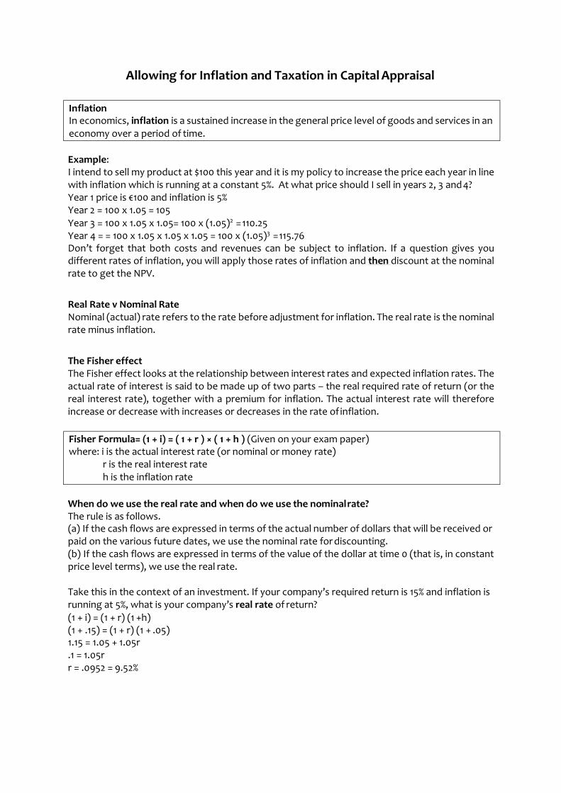
Example: I intend to sell my product at $100 this year and it is my policy to increase the price each year in line with inflation which is running at a constant 5%. At what price should I sell in years 2, 3 and 4? Year 1 price is €100 and inflation is 5% Year 2 = 100 x 1.05 = 105

Year 3 = 100 x 1.05 x 1.05= 100 x (1.05)2 = 110.25 Year 4 = = 100 x 1.05 x 1.05 x 1.05 = 100 x (1.05)3 = 115.76 Don’t forget that both costs and revenues can be subject to inflation. If a question gives you different rates of inflation, you will apply those rates of inflation and then discount at the nominal rate to get the NPV.

Real Rate v Nominal Rate Nominal (actual) rate refers to the rate before adjustment for inflation. The real rate is the nominal rate minus inflation.

The Fisher effect The Fisher effect looks at the relationship between interest rates and expected inflation rates. The actual rate of interest is said to be made up of two parts – the real required rate of return (or the real interest rate), together with a premium for inflation. The actual interest rate will therefore increase or decrease with increases or decreases in the rate of inflation.

When do we use the real rate and when do we use the nominal rate? The rule is as follows. (a) If the cash flows are expressed in terms of the actual number of dollars that will be received or paid on the various future dates, we use the nominal rate for discounting. (b) If the cash flows are expressed in terms of the value of the dollar at time 0 (that is, in constant price level terms), we use the real rate.

Take this in the context of an investment. If your company’s required return is 15% and inflation is running at 5%, what is your company’s real rate of return?

(1 + i) = (1 + r) (1 +h) (1 + .15) = (1 + r) (1 + .05) 1.15 = 1.05 + 1.05r .1 = 1.05r r = .0952 = 9.52%

Inflation In economics, inflation is a sustained increase in the general price level of goods and services in an economy over a period of time.

Fisher Formula= (1 + i) = ( 1 + r ) × ( 1 + h ) (Given on your exam paper) where: i is the actual interest rate (or nominal or money rate)

r is the real interest rate h is the inflation rate

© Cenit Online 2015 60

Generally in your exam:

• Tax is payable at the stated rate one year in arrears

• Capital Allowances (Tax Allowable Depreciation Benefit) are used to reduce taxable profits • Net operating cash flows are taken as being taxable profits i.e. Sales Revenue – Costs.

N.B. Learn the NPV Layout and adjust as needed for the question you are asked.

Sample NPV Question Layout for a 4 year Project

Yr 0 Yr1 Yr2 Yr3 Yr4 Yr5

Investment (Deduct) (x)

Sales Revenue x x x x

Variable Costs (Deduct) x x x x

Fixed Costs (Deduct) x x x x

Cash Flow Before Tax x x x x

Tax Liability (Deduct) (x) (x) (x) (x)

Tax Allowable Depreciation benefit (Add Back) x x x x

After Tax Cash Flow (x) x x x x (x)

Working Capital (x) (x) (x) (x) (x) x

Scrap Value x

Net Cash Flows (x) x x x x (x)

Discount Factor @ x% 1 .xxx .xxx .xxx .xxx .xxx

Present Value (x) x x x x (x)

NPV X

Remember: Adjust this template to suit the question asked.

Not all questions will have all of these topics and some questions will have other topics.

Make a note of workings so examiner can find your calculations

Note; working capital in these questions is incremental. If I have invested €50,000 in Working capital in year 1 and require €60,000 in year 2, year 2 investment will be €10,000.

At the end of the project, working capital may be released back into the business so a cash inflow may be shown. Carefully read the question to see if this is the case.

Taxation is a means by which governments finance their expenditure by imposing charges on citizens and corporate entities.

© Cenit Online 2015 61

Calculation of Reducing Balance and Straight-Line Depreciation?

Reducing Balance Depreciate and asset with a 4 year life and a value of €100,000 at 25% on a reducing balance basis. Assume that the remaining value is written off at the end of the assets life.

Year Calculation Depreciation Balance

1 25% of 100,000 25,000 75,000

2 25% of €75,000 18,750 56,250

3 25% of 56,250 14,062 42,187

4 Remaining 42,187 0

Straight-line Depreciate and asset with a 4 year life and a value of €100,000 at 25% on a straight-line basis. Assume that the remaining value is written off at the end of the assets life.

Year Calculation Depreciation Balance

1 25% of 100,000 25,000 75,000

2 25% of 100,000 25,000 50,000

3 25% of 100,000 25,000 25,000

4 25% of 100,000 25,000 0

Watch for the rate of depreciation quoted, the treatment of final value, the treatment you are required to use.

© Cenit Online 2015 62

Capital Appraisal Calculation 1

Don’t forget your layout template.

Sample NPV Question Layout for a 4 year Project

Yr 0 Yr1 Yr2 Yr3 Yr4 Yr5

Investment (Deduct) (x)

Sales Revenue x x x x

Variable Costs (Deduct) x x x x

Fixed Costs (Deduct) x x x x

Cash Flow Before Tax x x x x

Tax Liability (Deduct) (x) (x) (x) (x)

Tax Allowable Depreciation benefit (Add Back) x x x x

After Tax Cash Flow (x) x x x x (x)

Working Capital (x) (x) (x) (x) (x) x

Scrap Value x

Net Cash Flows (x) x x x x (x)

Discount Factor @ x% 1 .xxx .xxx .xxx .xxx .xxx

Present Value (x) x x x x (x)

NPV X

Remember: Adjust this template to suit the question asked.

Not all questions will have all of these topics and some questions will have other topics.

Make a note of workings so examiner can find your calculations

Note; working capital in these questions is incremental. If I have invested €50,000 in Working capital in year 1 and require €60,000 in year 2, year 2 investment will be €10,000.

At the end of the project, working capital may be released back into the business so a cash inflow may be shown. Carefully read the question to see if this is the case.

Now that you have all the basics covered we will look next at a full exam style question.

© Cenit Online 2015 63

Pilot Paper Q1

© Cenit Online 2015 64

© Cenit Online 2015 65

© Cenit Online 2015 66

Specimen Paper Q4

Capital Appraisal Calculation 2

Past Exam Questions on topics covered to date

Lectures 1 – 3

Past Exam Questions in this area

Paper Question Topic

April 2013 Q1 NPV

April 2012 Q1 NPV / Payback

August 2010 Q5 (a) Management Accounting

April 2010 Q1 NPV / Payback

Aug 2009 Q1 NPV / Payback

April 2008 Q1 NPV

Pilot Paper Q1 NPV / Payback

Q3 (a) Not for Profit Orgs

Q3 (b) Sources of Finance

© Cenit Online 2015 67

Allowing for Risk in Capital Appraisal

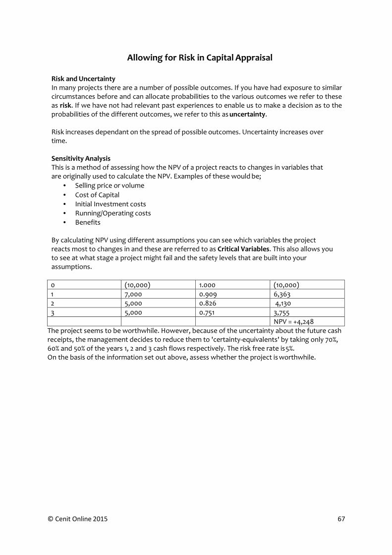
Risk and Uncertainty In many projects there are a number of possible outcomes. If you have had exposure to similar circumstances before and can allocate probabilities to the various outcomes we refer to these as risk. If we have not had relevant past experiences to enable us to make a decision as to the probabilities of the different outcomes, we refer to this as uncertainty.

Risk increases dependant on the spread of possible outcomes. Uncertainty increases over time.

Sensitivity Analysis This is a method of assessing how the NPV of a project reacts to changes in variables that are originally used to calculate the NPV. Examples of these would be;

• Selling price or volume

• Cost of Capital

• Initial Investment costs

• Running/Operating costs

• Benefits

By calculating NPV using different assumptions you can see which variables the project reacts most to changes in and these are referred to as Critical Variables. This also allows you to see at what stage a project might fail and the safety levels that are built into your assumptions.

0 (10,000) 1.000 (10,000)

1 7,000 0.909 6,363

2 5,000 0.826 4,130

3 5,000 0.751 3,755 NPV = +4,248 The project seems to be worthwhile. However, because of the uncertainty about the future cash receipts, the management decides to reduce them to 'certainty-equivalents' by taking only 70%, 60% and 50% of the years 1, 2 and 3 cash flows respectively. The risk free rate is 5%. On the basis of the information set out above, assess whether the project is worthwhile.

© Cenit Online 2015 68