Checking Assumptions in theCox Proportional Hazards

Regression ModelBrenda Gillespie, Ph.D.University of Michigan

Presented at the 2006 Midwest SAS Users Group (MWSUG)Dearborn, Michigan

October 22-24, 2006© 2006 Center for Statistical Consultation and Research, University of Michigan

All rights reserved.

SD08

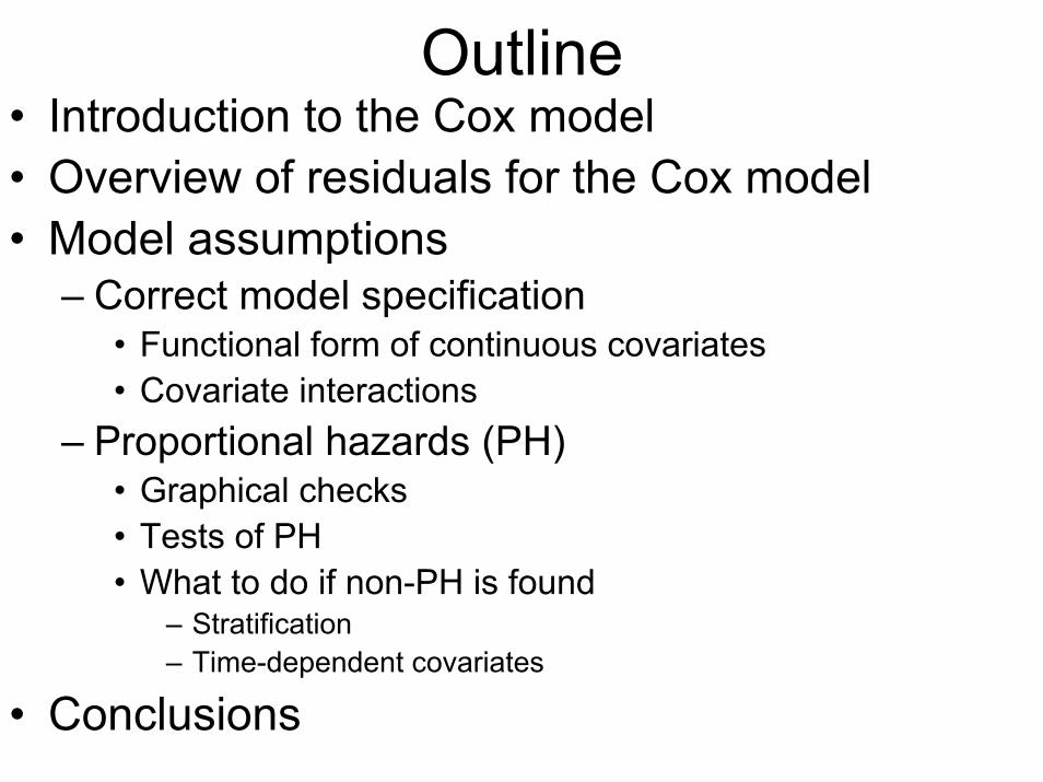
Outline• Introduction to the Cox model• Overview of residuals for the Cox model• Model assumptions

– Correct model specification• Functional form of continuous covariates• Covariate interactions

– Proportional hazards (PH)• Graphical checks• Tests of PH• What to do if non-PH is found

– Stratification– Time-dependent covariates

• Conclusions

Survival Analysis

• Methods to analyze “time to event” data.• Useful for many different applications

– Time to death from disease diagnosis– Length of hospital stay– Cost of insurance claims.

Time origin Event

Time origin Censored value

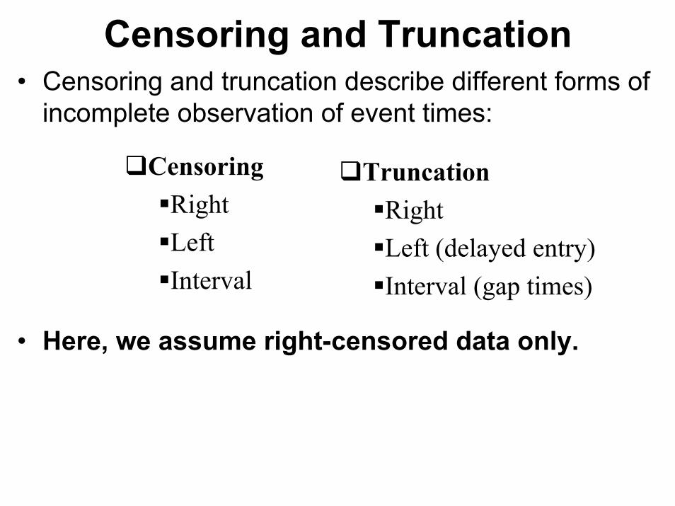
Censoring and Truncation• Censoring and truncation describe different forms of

incomplete observation of event times:

• Here, we assume right-censored data only.

CensoringRightLeftInterval

TruncationRightLeft (delayed entry)Interval (gap times)

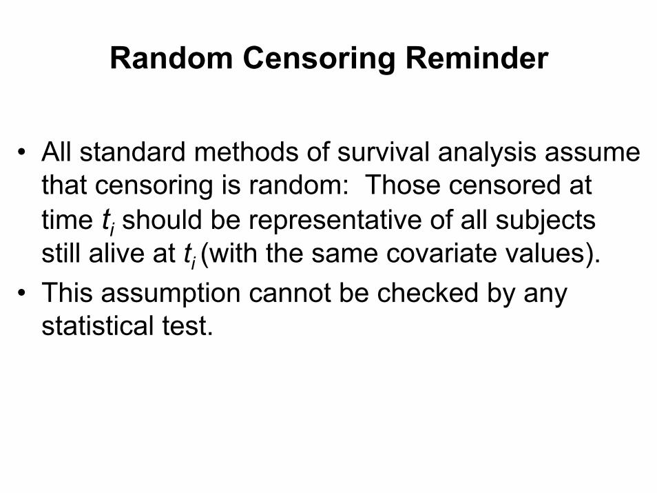
Random Censoring Reminder

• All standard methods of survival analysis assume that censoring is random: Those censored at time ti should be representative of all subjects still alive at ti (with the same covariate values).

• This assumption cannot be checked by any statistical test.

Cox Regression Model

where h(t ; x) is the hazard function at time t for a subject with covariate values x1, … xk,

h0(t) is the baseline hazard function, i.e., the hazard function when all covariates equal zero.

exp is the exponential function (exp(x)= ex),xi is the ith covariate in the model, andβi is the regression coefficient for the ith covariate, xi.

h t x h t x xo k k( ; ) ( )exp{ }= + +β β1 1 L

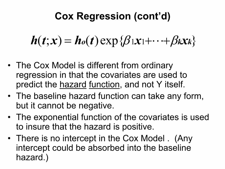
Cox Regression (cont’d)

• The Cox Model is different from ordinary regression in that the covariates are used to predict the hazard function, and not Y itself.

• The baseline hazard function can take any form, but it cannot be negative.

• The exponential function of the covariates is used to insure that the hazard is positive.

• There is no intercept in the Cox Model . (Any intercept could be absorbed into the baseline hazard.)

h t x h t x xo k k( ; ) ( )exp{ }= + +β β1 1 L

Cox Regression (cont’d)

h(t, xi)

t

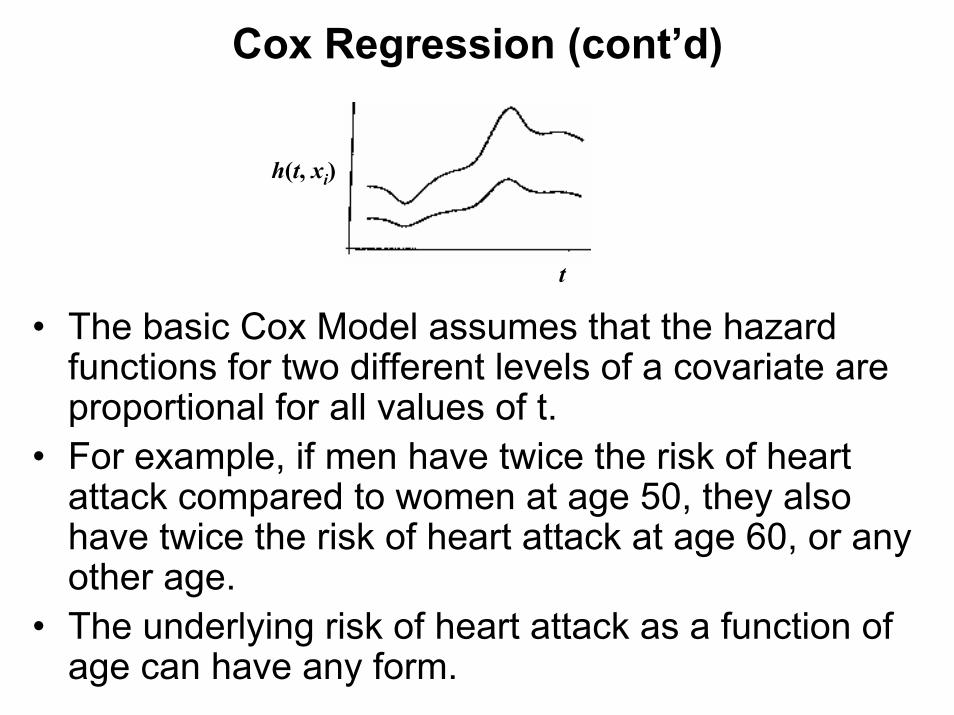
• The basic Cox Model assumes that the hazard functions for two different levels of a covariate are proportional for all values of t.

• For example, if men have twice the risk of heart attack compared to women at age 50, they also have twice the risk of heart attack at age 60, or any other age.

• The underlying risk of heart attack as a function of age can have any form.

Proportional HazardsTo see the proportional hazards property analytically,take the ratio of h(t;x) for two different covariate values:

ho(t) cancels out => the ratio of those hazards is the sameat all time points.For a single dichotomous covariate, say with values 0 and 1,the hazard ratio is

)}()(exp{= }exp{)(}exp{)(

);();(

111

110

110

jkikkji

jkkj

ikki

j

i

xxxxxxthxxth

xthxth

−++−++++

=

ββββββ

L

L

L

ββ

β

β

eee

etheth

xthxth

=====

00*0

1*0

)()(

)0;()1;(

Software for Cox Regression: PHREG

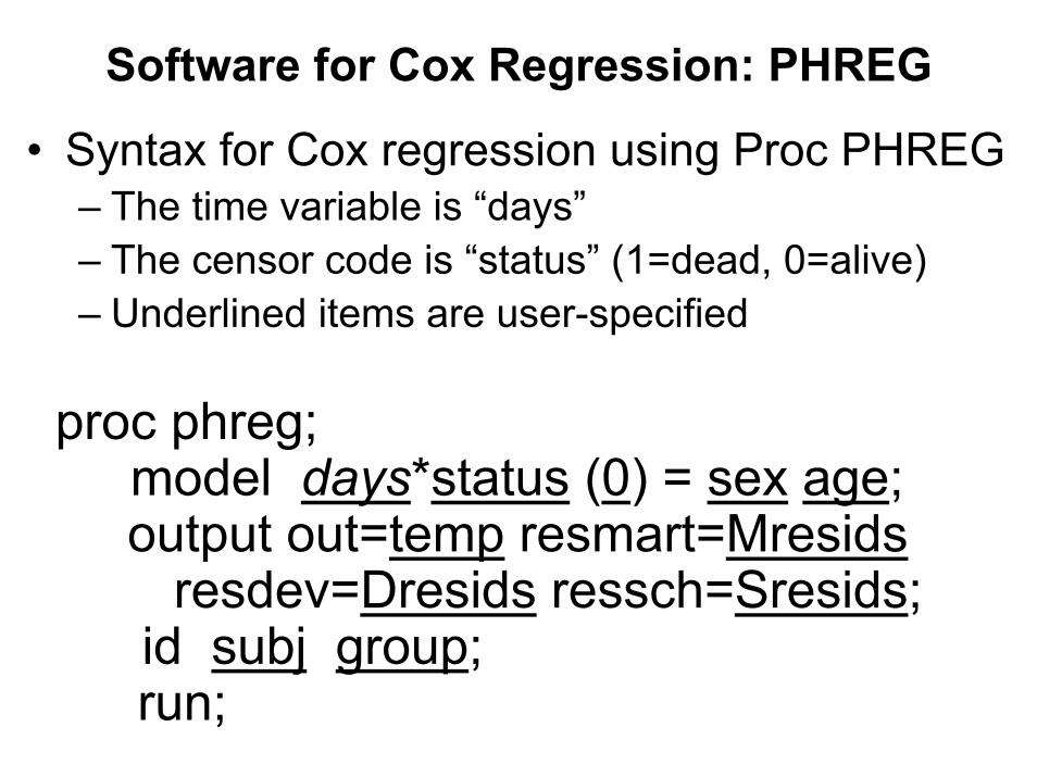
• Syntax for Cox regression using Proc PHREG– The time variable is “days”– The censor code is “status” (1=dead, 0=alive)– Underlined items are user-specified

proc phreg;model days*status (0) = sex age;output out=temp resmart=Mresids

resdev=Dresids ressch=Sresids;id subj group;run;

Overview of Residuals for Cox Regression

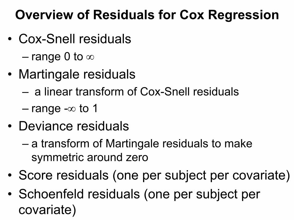
• Cox-Snell residuals – range 0 to ∞

• Martingale residuals– a linear transform of Cox-Snell residuals – range -∞ to 1

• Deviance residuals – a transform of Martingale residuals to make

symmetric around zero• Score residuals (one per subject per covariate)• Schoenfeld residuals (one per subject per

covariate)

Common Residual Plots• Plot martingale residuals vs continuous

covariates – to check functional form of covariates

• Plot deviance residuals vs Observation # – to check for outliers

• Plot Schoenfeld residuals for each covariate, vs Time or log(Time)– to check proportional hazards (PH)

• Note: Censoring and categorical covariates can produce banded residual patterns that do not reflect any problem with the model.

Martingale Residuals

• Skewed• Near 1 ⇒ “died too soon”; Large negative

⇒ “lived too long”• Plots of residuals vs. continuous

covariates: Patterns may suggest continuous variables not properly fit

Mar

tinga

le R

esid

uals

-7

-6

-5

-4

-3

-2

-1

0

1

Observation Number

0 50 100 150 200 250 300 350 400 450 500

Example of Martingale Residuals

Deviance Residuals

• Roughly symmetrically distributed around zero, with approximate s.d. = 1.0

• Positive values ⇒ “died too soon”• Negative values ⇒ “lived too long”• Very large or small values ⇒ outliers

• This is the only plot that is useful for checking outliers.

Dev

ianc

e R

esid

uals

-3

-2

-1

0

1

2

3

4

Observation Number

0 50 100 150 200 250 300 350 400 450 500

Example of Deviance Residuals

Schoenfeld Residuals• Schoenfeld residuals are computed with one

per observation per covariate.– Only defined at observed event times– For the ith subject and kth covariate, the estimated

Schoenfeld residual, rik, is given by (notation from Hosmer and Lemeshow)

– Where xik is the value of the kth covariate for individual i, and

– is a weighted mean of covariate values for those in the risk set at the given event time.

– A positive value of rik shows an X value that is higher than expected at that death time.

kwikik ixxr ˆˆ −=

kwix

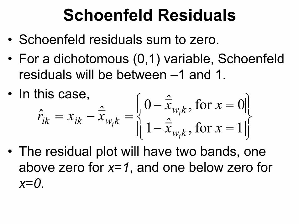
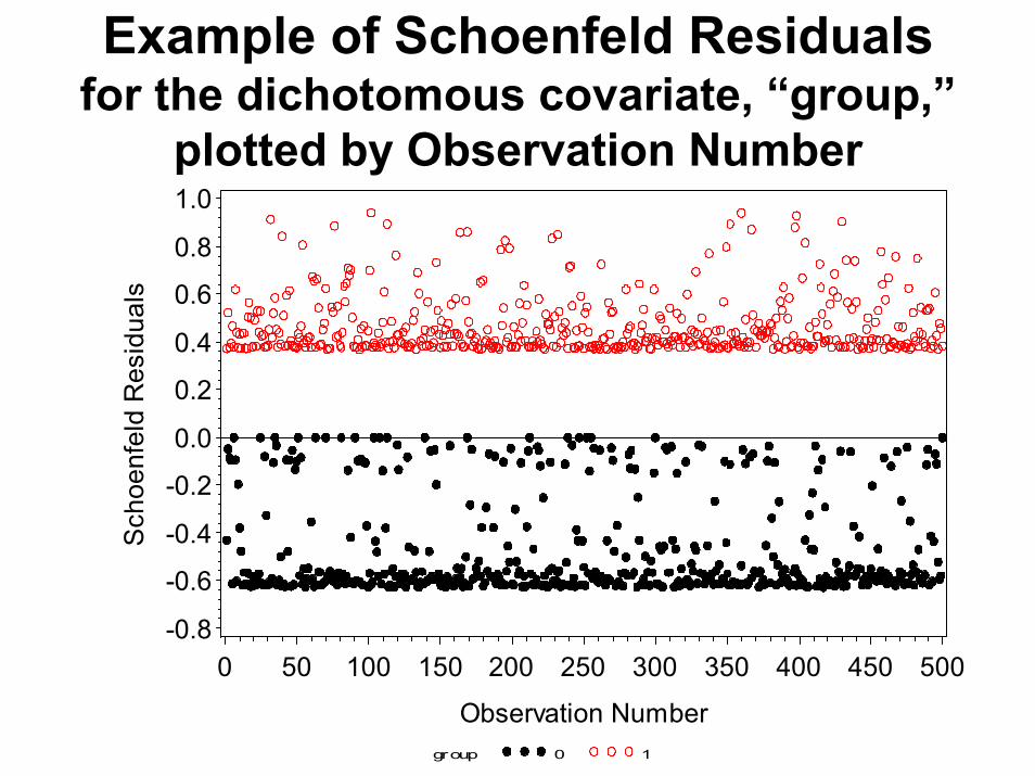
Schoenfeld Residuals• Schoenfeld residuals sum to zero.• For a dichotomous (0,1) variable, Schoenfeld

residuals will be between –1 and 1.• In this case,

• The residual plot will have two bands, one above zero for x=1, and one below zero for x=0.

=−

=−=−=

1for ,ˆ10for ,ˆ0ˆˆ

xxxx

xxrkw

kwkwikik

i

ii

group 0 1

Sch

oenf

eld

Res

idua

ls

-0.8

-0.6

-0.4

-0.2

0.0

0.2

0.4

0.6

0.8

1.0

Observation Number

0 50 100 150 200 250 300 350 400 450 500

Example of Schoenfeld Residuals for the dichotomous covariate, “group,”

plotted by Observation Number

group 0 1

Sch

oenf

eld

Res

idua

ls

-0.8

-0.6

-0.4

-0.2

0.0

0.2

0.4

0.6

0.8

1.0

Time

0 1 2 3 4 5 6

Example of Schoenfeld Residuals for the dichotomous covariate, “group,”

plotted by Time

The increasing patternIndicates non-PH.

An Example of Martingale and Deviance Residuals with non-PH

• Outcome: Time to death• Covariate: treatment group (labels 0 and 1)• The next 3 slides show

– Kaplan-Meier plot for the two groups– Martingale residuals– Deviance residuals

group 0 1

Sur

viva

l Pro

babi

lity

0.00.10.20.30.40.50.60.70.80.91.0

Time

0 1 2 3 4 5 6

Example: KM Plot shows Crossing Survival Functions (non-PH)

Group=0 has more “early deaths,”but also more longer lifetimes than Group=1.

group 0 1

Mar

tinga

le R

esid

uals

-7

-6

-5

-4

-3

-2

-1

0

1

Observation Number

0 50 100 150 200 250 300 350 400 450 500

Martingale Residuals

Group=0 (solid dots) has both the earliest deaths (top) and the longest surviving values (bottom).

group 0 1

Dev

ianc

e R

esid

uals

-3

-2

-1

0

1

2

3

4

Observation Number

0 50 100 150 200 250 300 350 400 450 500

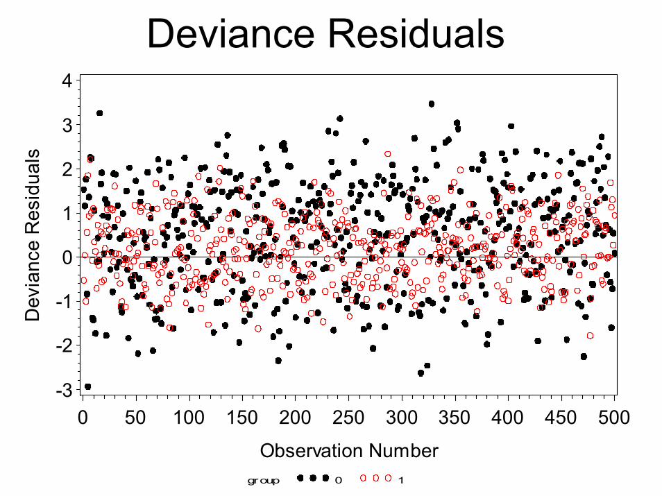
Deviance Residuals

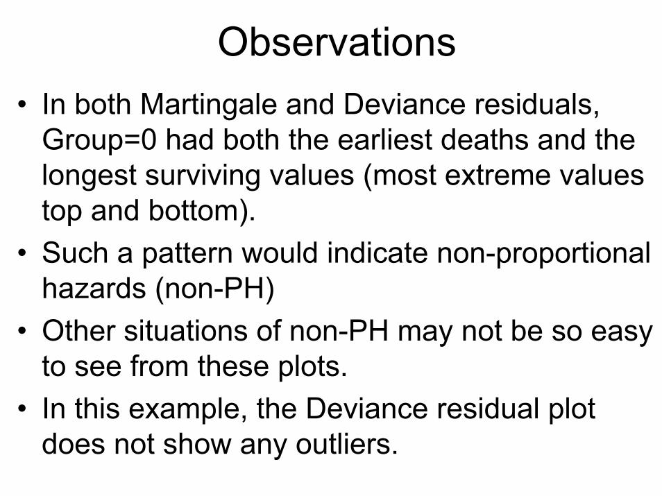
Observations• In both Martingale and Deviance residuals,

Group=0 had both the earliest deaths and the longest surviving values (most extreme values top and bottom).

• Such a pattern would indicate non-proportional hazards (non-PH)

• Other situations of non-PH may not be so easy to see from these plots.

• In this example, the Deviance residual plot does not show any outliers.

Assumptions of the Cox Model• Structure of the model is assumed correct

– Model is multiplicative (e.g., vs additive)– All relevant covariates have been included– We will not consider these assumptions here

• Functional form– Do we have the correct functional form for

continuous covariates?– Are there any significant interactions?

• Is the Proportional Hazards assumption met? If not, what are the options?

Assessing Functional Form of Continuous Covariates

• Often we assume continuous covariates have a linear form. However, this assumption should always be checked. We give 3 ways to check:

• Method 1 (try X categorical):– Categorize X into ≥4 intervals, say by quantiles.– Create dummy variables for the categories and

fit a model with these dummy variables. – Plot β estimates by X interval midpoints, with

β=0 for the reference category. – Look at the shape, and model X accordingly

(e.g., linear, quadratic, threshold).

Plot of Beta Estimates by Age Category Midpoints

0. 0

0. 1

0. 2

0. 3

0. 4

0. 5

0. 6

0. 7

0. 8

0. 9

1. 0

1. 1

1. 2

1. 3

1. 4

1. 5

1. 6

Age (years)30 40 50 60 70

Pattern looks linear

Assessing Functional Form (cont’d)• Method 2 (loess line through martingale residuals):

– Output martingale residuals from a model WITHOUT X. (proc phreg; model …; output out=temp resmart=resids;)

– Fit a loess line through the martingale residuals, as a function of X.(ods output ScoreResults=temp2; proc loess data=temp; model resids=X; score; run;)

– Plot martingale residuals (with loess curve) by X.(proc gplot data=temp2; plot resids*X p_resids*X / overlay; run;)

– Model X as appropriate (e.g., linear, quadratic, threshold), and re-check.

Plot of Martingale Residuals by Age, with Loess Line (Age not in model)

Mar

tinga

le R

esid

uals

-3

-2

-1

0

1

Age (years)30 40 50 60 70

Reference line at 0

Looks like HR increases with age

Loess line

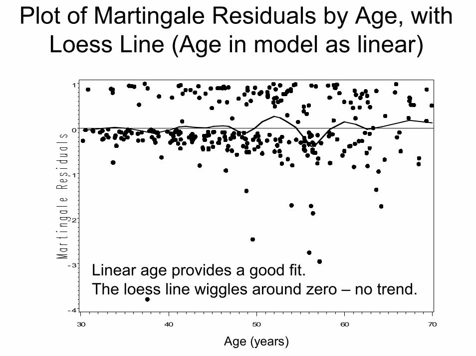
Plot of Martingale Residuals by Age, with Loess Line (Age in model as linear)

-4

-3

-2

-1

0

1

Age (years)30 40 50 60 70

Linear age provides a good fit.The loess line wiggles around zero – no trend.

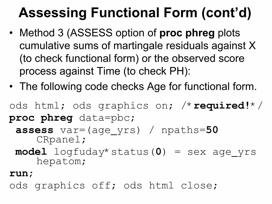
Assessing Functional Form (cont’d)• Method 3 (ASSESS option of proc phreg plots

cumulative sums of martingale residuals against X (to check functional form) or the observed score process against Time (to check PH):

• The following code checks Age for functional form.

ods html; ods graphics on; /*required!*/proc phreg data=pbc;assess var=(age_yrs) / npaths=50

CRpanel;model logfuday*status(0) = sex age_yrs

hepatom;run;ods graphics off; ods html close;

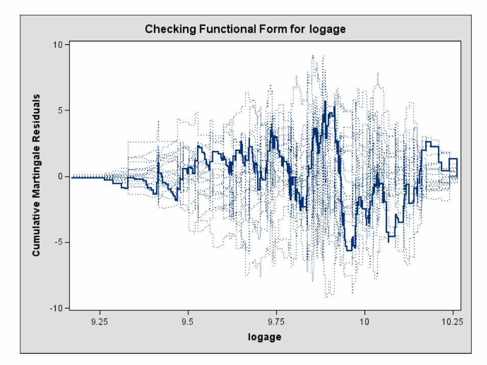
Assessing the Cumulative Martingale Residual Plot

• The plot shows the observed curve for Age to be within the distribution of the simulated cumulative martingale residual curves, indicating acceptable fit with linear age.

• Note that ASSESS cannot check functional form with a variable out of the model. It must be included in the model in some form.

• To try to illustrate a bad fit, we try log(Age), Age2, and Age5. Only Age5 shows poor fit.

The Resample option of ASSESS

• The Resample option of ASSESS gives– a test of the functional form– A test of PH

• Tests are based on a Kolmogorov-type supremum test using 1000 simulated patterns.

• ASSESS var=(age_yrs) PH / resample;

Supremum Test for Functional Form

MaximumAbsolute Pr >

Variable Value Reps MaxAbsValage_yrs 6.0767 1000 0.6640

Supremum Test for Proportionals Hazards Assumption

MaximumAbsolute Pr >

Variable Value Reps MaxAbsValSEX 0.5985 1000 0.9930HEPATOM 0.5504 1000 0.9920age_yrs 0.5587 1000 0.9950

Summary of ASSESS Option• The ASSESS option is a useful tool, but

should be used in conjunction with other checks for functional form and PH.

• The cumulative martingale residual plots are not very sensitive for fine-tuning functional form. They can show grossly incorrect forms.

• We recommend martingale residuals (not cumulative), with a loess line to show functional form.

Covariate Interactions

• In many types of models, covariate interactions can be a challenge to interpret and present.

• With linear or logistic regression models, interaction plots are useful.

• With the Cox model, interaction plots, like variable effects, are based on Hazard Ratios.

Two dichotomous covariates: With interaction:

h(t;x) = ho(t) exp{β1x1 + β2x2 + β3x1x2}x1, x2 h(t;x)

A, M 0, 1 ho(t) eβ2

log h(t, x) 1, 1 ho(t) eβ1 + β2 + β3

0, 0 ho(t)1, 0 ho(t) eβ1

Β, Μ

Α, F

B, F

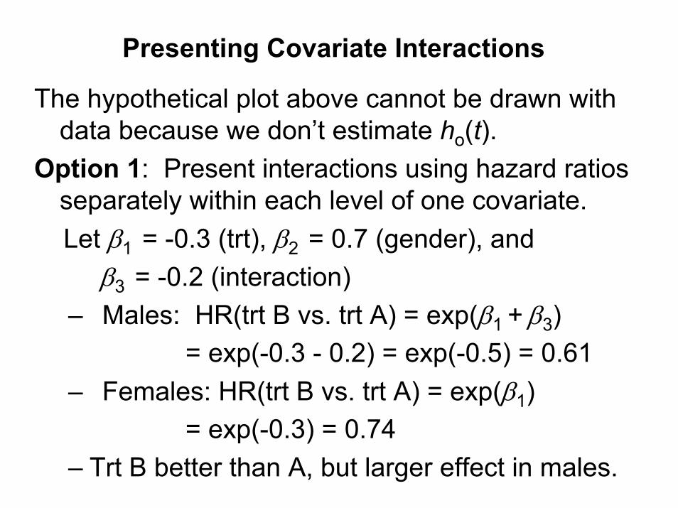
Presenting Covariate Interactions

The hypothetical plot above cannot be drawn with data because we don’t estimate ho(t).

Option 1: Present interactions using hazard ratios separately within each level of one covariate. Let β1 = -0.3 (trt), β2 = 0.7 (gender), and

β3 = -0.2 (interaction)– Males: HR(trt B vs. trt A) = exp(β1 + β3)

= exp(-0.3 - 0.2) = exp(-0.5) = 0.61– Females: HR(trt B vs. trt A) = exp(β1)

= exp(-0.3) = 0.74– Trt B better than A, but larger effect in males.

Presenting Covariate Interactions

Option 2: Compare all subgroups to a single baseline group. These hazard ratios can be plotted. The reference group is Females on treatment A.

HRMales

A 2.0 = eβ2

B 1.2 = eβ1 + β2 + β3

Females A 1.0B 0.7 = eβ1

2HR

A1B

FemalesMales

Presenting Covariate Interactions with Continuous Covariates

• For an interaction between a continuous and a categorical covariate, plot the HR by the continuous covariate, with separate lines for the levels of the categorical covariate.

• For an interaction between two continuous covariates, plot the HR by one of the the continuous covariate, with separate lines for selected values of the other covariate.

A striking interaction between age and severe edema in the PBC dataset.

0

50

100

150

200

250

Age (years)30 40 50 60 70

Severe Edema

No Edema

Reference category is Age=30, No Edema

Checking Proportional Hazards (PH)

• Graphical methods to check PH

• Using time-dependent covariates to test PH

• Other tests for PH

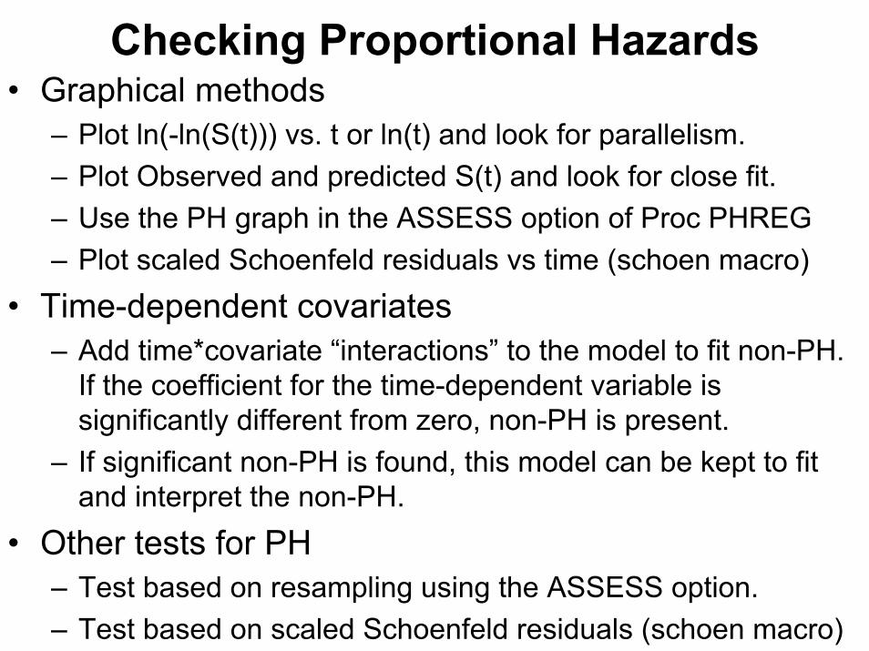
Checking Proportional Hazards• Graphical methods

– Plot ln(-ln(S(t))) vs. t or ln(t) and look for parallelism.– Plot Observed and predicted S(t) and look for close fit.– Use the PH graph in the ASSESS option of Proc PHREG – Plot scaled Schoenfeld residuals vs time (schoen macro)

• Time-dependent covariates– Add time*covariate “interactions” to the model to fit non-PH.

If the coefficient for the time-dependent variable is significantly different from zero, non-PH is present.

– If significant non-PH is found, this model can be kept to fit and interpret the non-PH.

• Other tests for PH – Test based on resampling using the ASSESS option.– Test based on scaled Schoenfeld residuals (schoen macro)

Proportional Hazards: Graphical Check #1Plot ln(-ln(S(t))) vs. t or ln(t) and look for parallelism.

Week

FIN = 0FIN = 1

log(-log S(t))

Parallel curves PHUse Kaplan-Meier estimate for S(t).This plot shows reasonable fit to the PH assumption.

⇒

Proportional Hazards: Graphical Check #1

• Interpreting plots is subjective. In general, conclude PH unless a distinct pattern of non-parallelism (e.g., crossing) is seen.

• Intertwined lines with no distinct pattern may simply indicate no difference between groups.

• Adjusting for other covariates may be needed.– Example: To check PH for treatment, adjusted for age:– Run a Cox model with age as a covariate, stratified by

treatment.– Output the estimated survivor functions for each treatment

group at the overall mean age.– Plot ln(-ln( (t))) for each treatment group vs ln(t) and

check for parallelism.S

SAS® Code for log(-log(S(t))) PlotsUnadjusted PH check for Treatment:

Proc lifetest data=data1 plots=(lls);time days*status(0); strata treat; run;

Adjusted PH check for Treatment, adjusted for Age:data covs; age=52; run; /*Overall mean age*/

Proc phreg data=pbc;model days*status(0) = age;strata treat;baseline out=temp covariates=covs loglogs=lls;

Proc plot data=temp; plot lls*days=treat; run;

Proportional Hazards: Graphical Check #2Plot Observed and predicted S(t) and look for close fit.

(Only feasible with small number of covariates.)

• Predicted is from Cox model. Observed is KM.(Figure from Kleinbaum)

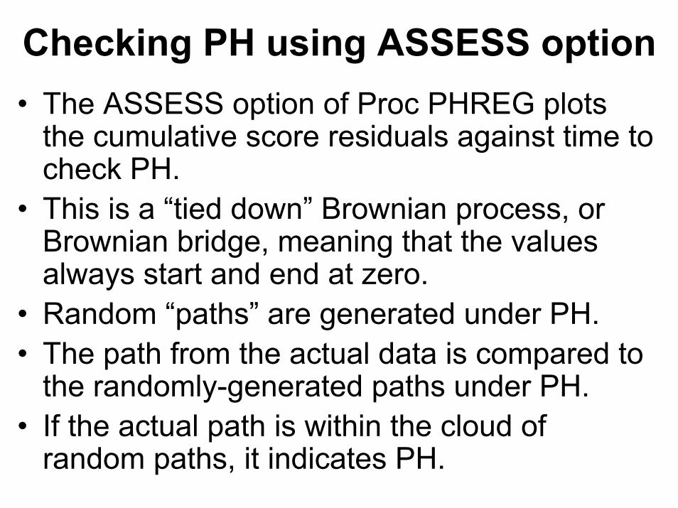
Checking PH using ASSESS option• The ASSESS option of Proc PHREG plots

the cumulative score residuals against time to check PH.

• This is a “tied down” Brownian process, or Brownian bridge, meaning that the values always start and end at zero.

• Random “paths” are generated under PH.• The path from the actual data is compared to

the randomly-generated paths under PH.• If the actual path is within the cloud of

random paths, it indicates PH.

Checking PH using ASSESS option

Clear evidence of non-PH.

But the form of the non-PH isnot clear.

Cloud of random paths

Path from the actual data

Checking PH using macro SCHOEN• The SAS® macro, SCHOEN, gives a different

graphical check for PH.• Consider the possibility that the β coefficient for a

given covariate, βk, changes over time, thus giving a non-constant hazard ratio.

• Macro SCHOEN uses a scaled Schoenfeld residual, multiplying the vector of Schoenfeld residuals by the inverse of their covariance matrix.

• This scaled residual, rik*, added to βk, is an estimate of

the time-dependent β coefficient: rik* + βk ≈ βk(ti).

• rik* + βk is plotted against time, or a function of time.

• PH is indicated by a flat pattern around Y=0.• Non-PH is indicated by any deviation from a flat line at

Y=0.

Which function of time?• The Schoenfeld residuals can be plotted against

any function of time, such as raw, log-transformed, or rank-transformed.

• The pattern shown over time indicates the form of non-PH.

• Different functions show different shapes, and some may be better for highlighting non-PH for a particular variable. Try more than one.

• Options available in the “schoen” macro are:– Raw time– Rank-transformed time– Time transformed by (1 - Kaplan-Meier) (Similar to

probability integral transformation.)

Scal ed resi dual s(Bt ) as a f cn of t i me.

Xvars= groupschoen macro: event =cens t i me=t st rat a=

-3

-2

-1

0

1

2

3

4

5

1-Overal l Kapl an-Mei er

0 0. 1 0. 2 0. 3 0. 4 0. 5 0. 6 0. 7 0. 8 0. 9 1

Checking PH with macro SCHOEN (KM-transformed time scale)

Non-PH shown by increasing trend. Note the top and bottom lines are the same Schoenfeld residuals shown on slide 20.

Interpreting the SCHOEN Plot• The previous plot clearly shows an

increasing pattern, suggesting linear.• The true hazard ratio is linearly

increasing in log(t). • The SCHOEN plot is more useful than

the ASSESS plot in showing the appropriate functional form for a non-PH relationship.

Scal ed resi dual s(Bt ) as a f cn of t i me.

Xvars= groupschoen macro: event =cens t i me=t st rat a=

-4

-3

-2

-1

0

1

2

3

4

5

t

0 1 2 3 4 5 6 7 8

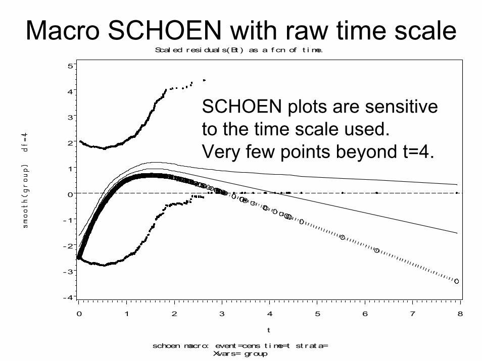
Macro SCHOEN with raw time scale

SCHOEN plots are sensitive to the time scale used. Very few points beyond t=4.

Scal ed resi dual s(Bt ) as a f cn of t i me.

Xvars= groupschoen macro: event =cens t i me=t st rat a=

-3

-2

-1

0

1

2

3

4

5

Rank f or Var i abl e t

0 100 200 300 400 500 600 700 800 900 1000

Macro SCHOEN with rank time scaleIncreasing trend, similar to that seen in KM time scale.

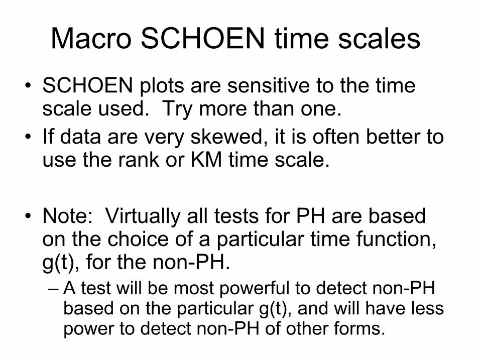
Macro SCHOEN time scales• SCHOEN plots are sensitive to the time

scale used. Try more than one.• If data are very skewed, it is often better to

use the rank or KM time scale.

• Note: Virtually all tests for PH are based on the choice of a particular time function, g(t), for the non-PH. – A test will be most powerful to detect non-PH

based on the particular g(t), and will have less power to detect non-PH of other forms.

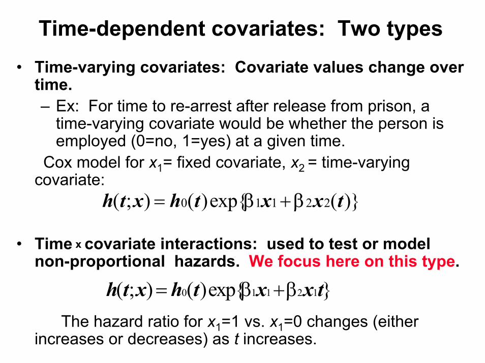
Time-dependent covariates: Two types• Time-varying covariates: Covariate values change over

time.– Ex: For time to re-arrest after release from prison, a

time-varying covariate would be whether the person is employed (0=no, 1=yes) at a given time.

Cox model for x1= fixed covariate, x2 = time-varying covariate:

• Time x covariate interactions: used to test or model non-proportional hazards. We focus here on this type.

The hazard ratio for x1=1 vs. x1=0 changes (either increases or decreases) as t increases.

h t x h t x x t( ; ) ( )exp{ ( )}= +0 1 1 2 2β β

h t x h t x x t( ; ) ( )exp{ }= +0 1 1 2 1β β

Time*Covariate Interactionsh(t;x) = ho(t) exp{β1x + β2x t }

β2 >0 => HR increasing with timeβ2 <0 => HR decreasing with timeβ2 =0 => HR constant with time => PH

Add x* t to the model to test PH (test H0: β2=0).If β2 significant, then leave x* t in the model

(to model the non-PH).Some authors suggest other interactions, e.g.,

x*log(t) or x*I[t>c] (heavyside function). Use whatever fits best.

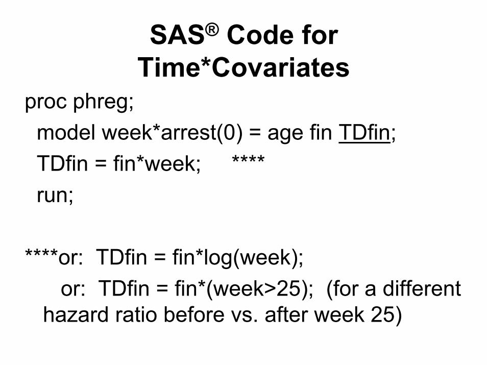
SAS® Code for Time*Covariates

proc phreg; model week*arrest(0) = age fin TDfin;TDfin = fin*week; ****run;

****or: TDfin = fin*log(week);or: TDfin = fin*(week>25); (for a different

hazard ratio before vs. after week 25)

Stratification vs. Time*Covariate Interactions for Handling Non-PH

• Time*Covariate Interaction– Must choose a particular form, such as x*t or x*log(t).– If this form is correct, yields more efficient estimates of other

βs. (robustness vs. efficiency)– The changing HR over time can be presented and

interpreted.• Stratification

– Takes less computation time– Models any non-PH relationship, not just specific forms– No inference is possible for the stratification variable; only

makes sense for “nuisance variables”.

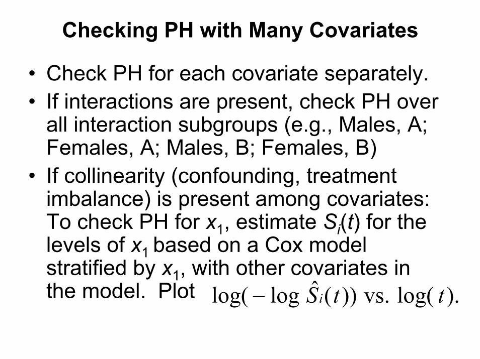
Checking PH with Many Covariates

• Check PH for each covariate separately.• If interactions are present, check PH over

all interaction subgroups (e.g., Males, A; Females, A; Males, B; Females, B)

• If collinearity (confounding, treatment imbalance) is present among covariates: To check PH for x1, estimate Si(t) for the levels of x1 based on a Cox model stratified by x1, with other covariates in the model. Plot ).log( vs.))(ˆloglog( ttSi−

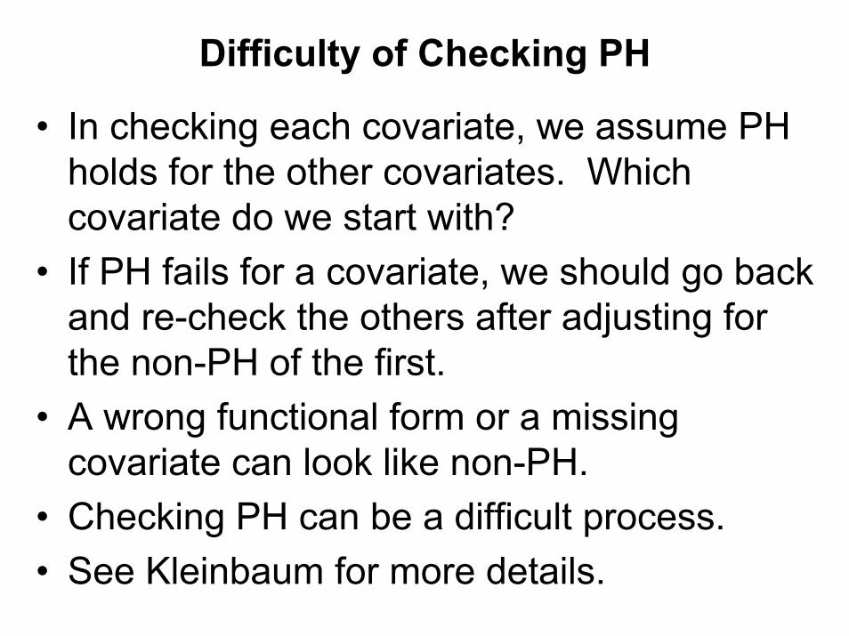
Difficulty of Checking PH

• In checking each covariate, we assume PH holds for the other covariates. Which covariate do we start with?

• If PH fails for a covariate, we should go back and re-check the others after adjusting for the non-PH of the first.

• A wrong functional form or a missing covariate can look like non-PH.

• Checking PH can be a difficult process.• See Kleinbaum for more details.

Summary and Recommendations• Check for outliers

– Deviance residual plot• Check for functional form of continuous covariates

– Martingale residual plots• Check for non-PH

– Use log(-log(S(t))) plots (either unadjusted or adjusted)– Test time*covariate interactions– Use the “schoen” macro to plot βk(ti) by time

• Checking assumptions takes time. Take the time.• Checking can be never-ending, so balance is

needed. Some checking is better than none.

The Cox Modeler’s Blessing

May your continuous covariates all be linear,

and may all your covariates satisfy the proportional hazards assumption …

References•Therneau TM and Grambsch PM. (2000). Modeling Survival Data: Extending the Cox Model, Springer.•Allison PD. (1995), Survival Analysis Using the SAS System: A Practical Guide, SAS Institute Inc.•Klein JP and Moeschberger ML. (1997), Survival Analysis: Techniques for Censored and Truncated Data, Springer-Verlag.•Marubini E and Valsecchi MG. (1995), Analysing Survival Data from Clinical Trials and Observational Studies, John Wiley & Sons Ltd. •Hosmer DW Jr and Lemeshow S. (1999), Applied Survival Analysis, Wiley.•Kalbfleisch JD and Prentice RL. (2002), The Statistical Analysis of Failure Time Data, 2nd Edition, Wiley.

SAS and all other SAS Institute Inc. product or service names are registered trademarks or trademarks of SAS Institute Inc. in the USA and other countries. ® indicates USA registration.