Cox Proportional-Hazards Regression for Survival Data in R

An Appendix to An R Companion to Applied Regression, Second Edition

John Fox & Sanford Weisberg

last revision: 23 February 2011

Abstract

Survival analysis examines and models the time it takes for events to occur, termed survivaltime. The Cox proportional-hazards regression model is the most common tool for studying thedependency of survival time on predictor variables. This appendix to Fox and Weisberg (2011)briefly describes the basis for the Cox regression model, and explains how to use the survivalpackage in R to estimate Cox regressions.

1 Introduction

Survival analysis examines and models the time it takes for events to occur. The prototypical suchevent is death, from which the name “survival analysis” and much of its terminology derives, butthe ambit of application of survival analysis is much broader. Essentially the same methods areemployed in a variety of disciplines under various rubrics—for example, “event-history analysis”in sociology and “failure-time analysis” in engineering. In this appendix, therefore, terms such assurvival are to be understood generically.

Survival analysis focuses on the distribution of survival times. Although there are well knownmethods for estimating unconditional survival distributions, most interesting survival modeling ex-amines the relationship between survival and one or more predictors, usually termed covariatesin the survival-analysis literature. The subject of this appendix is the Cox proportional-hazardsregression model (introduced in a seminal paper by Cox, 1972), a broadly applicable and the mostwidely used method of survival analysis. Although we will not discuss them here, the survival pack-age in R (Therneau, 1999; Therneau and Grambsch, 2000) also contains all of the other commonlyemployed tools of survival analysis.1

As is the case for the other appendices to An R Companion to Applied Regression, we assumethat you have read the Companion and are therefore familiar with R2. In addition, we assumefamiliarity with Cox regression. We nevertheless begin with a review of basic concepts, primar-ily to establish terminology and notation. The second section of the appendix takes up the Coxproportional-hazards model with time-independent covariates. Time-dependent covariates are in-troduced in the third section. A fourth and final section deals with diagnostics.

1The survival package is one of the “recommended” packages that are included in the standard R distribution.The package must be loaded via the command library(survival).

2Most R functions used but not described in this appendix are discussed in Fox and Weisberg (2011). All the Rcode used in this appendix can be downloaded from http://tinyurl.com/carbook.

1

2 Basic Concepts and Notation

Let T represent survival time. We regard T as a random variable with cumulative distributionfunction P (t) = Pr(T ≤ t) and probability density function p(t) = dP (t)/dt. The more optimisticsurvival function S(t) is the complement of the distribution function, S(t) = Pr(T > t) = 1−P (t).A fourth representation of the distribution of survival times is the hazard function, which assessesthe instantaneous risk of demise at time t, conditional on survival to that time:

h(t) = lim∆t→0

Pr [(t ≤ T < t+ ∆t)|T ≥ t]∆t

=f(t)S(t)

Models for survival data usually employ the hazard function or the log hazard. For example,assuming a constant hazard, h(t) = ν, implies an exponential distribution of survival times, withdensity function p(t) = νe−νt. Other common hazard models include

log h(t) = ν + ρt

which leads to the Gompertz distribution of survival times, and

log h(t) = ν + ρ log(t)

which leads to the Weibull distribution of survival times. (See, for example, Cox and Oakes, 1984,sec. 2.3, for these and other possibilities.) In both the Gompertz and Weibull distributions, thehazard can either increase or decrease with time; moreover, in both instances, setting ρ = 0 yieldsthe exponential model.

A nearly universal feature of survival data is censoring, the most common form of which isright-censoring : Here, the period of observation expires, or an individual is removed from the study,before the event occurs—for example, some individuals may still be alive at the end of a clinicaltrial, or may drop out of the study for various reasons other than death prior to its termination. Anobservation is left-censored if its initial time at risk is unknown. Indeed, the same observation maybe both right and left-censored, a circumstance termed interval-censoring. Censoring complicatesthe likelihood function, and hence the estimation, of survival models.

Moreover, conditional on the value of any covariates in a survival model and on an individual’ssurvival to a particular time, censoring must be independent of the future value of the hazardfor the individual. If this condition is not met, then estimates of the survival distribution can beseriously biased. For example, if individuals tend to drop out of a clinical trial shortly before theydie, and therefore their deaths go unobserved, survival time will be over-estimated. Censoring thatmeets this requirement is noninformative. A common instance of noninformative censoring occurswhen a study terminates at a predetermined date.

3 The Cox Proportional-Hazards Model

Survival analysis typically examines the relationship of the survival distribution to covariates. Mostcommonly, this examination entails the specification of a linear-like model for the log hazard. Forexample, a parametric model based on the exponential distribution may be written as

log hi(t) = α+ β1xi1 + β2xi2 + · · ·+ βkxik

2

or, equivalently,hi(t) = exp(α+ β1xi1 + β2xi2 + · · ·+ βkxik)

that is, as a linear model for the log-hazard or as a multiplicative model for the hazard. Here, i isa subscript for observation, and the xs are the covariates. The constant α in this model representsa kind of log-baseline hazard, since log hi(t) = α [or hi(t) = eα] when all of the xs are 0. Thereare similar parametric regression models based on the other survival distributions described in thepreceding section.3

The Cox model, in contrast, leaves the baseline hazard function α(t) = log h0(t) unspecified:

log hi(t) = α(t) + β1xi1 + β2xi2 + · · ·+ βkxik

or, again equivalently,hi(t) = h0(t) exp(β1xi1 + β2xi2 + · · ·+ βkxik)

This model is semi-parametric because while the baseline hazard can take any form, the covariatesenter the model linearly. Consider, now, two observations i and i′ that differ in their x-values, withthe corresponding linear predictors

ηi = β1xi1 + β2xi2 + · · ·+ βkxik

andηi′ = β1xi′1 + β2xi′2 + · · ·+ βkxi′k

The hazard ratio for these two observations,

hi(t)hi′(t)

=h0(t)eηi

h0(t)eηi′

=eηi

eηi′

is independent of time t. Consequently, the Cox model is a proportional-hazards model.Remarkably, even though the baseline hazard is unspecified, the Cox model can still be esti-

mated by the method of partial likelihood, developed by Cox (1972) in the same paper in which heintroduced what came to called the Cox model. Although the resulting estimates are not as efficientas maximum-likelihood estimates for a correctly specified parametric hazard regression model, nothaving to make arbitrary, and possibly incorrect, assumptions about the form of the baseline hazardis a compensating virtue of Cox’s specification. Having fit the model, it is possible to extract anestimate of the baseline hazard (see below).

3.1 The coxph Function

The Cox proportional-hazards regression model is fit in R with the coxph function (located in thesurvival package):

> library(survival)

> args(coxph)

3The survreg function in the survival package fits the exponential model and other parametric accelerated failuretime models. Because the Cox model is now used much more frequently than parametric survival regression models,we will not describe survreg in this appendix. Enter ?survreg and see Therneau (1999) for details.

3

function (formula, data, weights, subset, na.action, init, control,method = c("efron", "breslow", "exact"), singular.ok = TRUE,robust = FALSE, model = FALSE, x = FALSE, y = TRUE, ...)

NULL

Most of the arguments to coxph, includingdata, weights, subset, na.action, singular.ok,model, x and y, are familiar from lm (see Chapter 4 of the Companion, especially Section 4.8).The formula argument is a little different. The right-hand side of the formula for coxph is thesame as for a linear model.4 The left-hand side is a survival object, created by the Surv function.In the simple case of right-censored data, the call to Surv takes the form Surv(time, event ),where time is either the event time or the censoring time, and event is a dummy variable coded1 if the event is observed or 0 if the observation is censored. See the on-line help for Surv for otherpossibilities.

Among the remaining arguments to coxph:

� init (initial values) and control are technical arguments: See the on-line help for coxph fordetails.

� method indicates how to handle observations that have tied (i.e., identical) survival times.The default "efron" method is generally preferred to the once-popular "breslow" method;the "exact" method is much more computationally intensive.

� If robust is TRUE, coxph calculates robust coefficient-variance estimates. The default is FALSE,unless the model includes non-independent observations, specified by the cluster functionin the model formula. We do not describe Cox regression for clustered data in this appendix.

3.2 An Illustration: Recidivism

The file Rossi.txt contains data from an experimental study of recidivism of 432 male prisoners,who were observed for a year after being released from prison (Rossi et al., 1980).5 The followingvariables are included in the data; the variable names are those used by Allison (1995), from whomthis example and variable descriptions are adapted:

� week: week of first arrest after release, or censoring time.

� arrest: the event indicator, equal to 1 for those arrested during the period of the study and0 for those who were not arrested.

� fin: a factor, with levels yes if the individual received financial aid after release from prison,and no if he did not; financial aid was a randomly assigned factor manipulated by the re-searchers.

� age: in years at the time of release.

� race: a factor with levels black and other.4There are, however, special functions cluster and strata that may be included on the right side of the model

formula. The cluster function is used to specify non-independent observations (such as several individuals in thesame family), and the strata function may be used to divide the data into sub-groups with potentially differentbaseline hazard functions, as explained in Section 5.1.

5The data file Rossi.txt is available on the web site for the Companion: See below.

4

� wexp: a factor with levels yes if the individual had full-time work experience prior to incar-ceration and no if he did not.

� mar: a factor with levels married if the individual was married at the time of release and notmarried if he was not.

� paro: a factor coded yes if the individual was released on parole and no if he was not.

� prio: number of prior convictions.

� educ: education, a categorical variable coded numerically, with codes 2 (grade 6 or less), 3(grades 6 through 9), 4 (grades 10 and 11), 5 (grade 12), or 6 (some post-secondary).6

� emp1 – emp52: factors coded yes if the individual was employed in the corresponding week ofthe study and no otherwise.

We read the data file into a data frame, and print the first few observations (omitting thevariables emp1 – emp52, which are in columns 11–62 of the data frame):

> url <- "http://socserv.mcmaster.ca/jfox/Books/Companion/data/Rossi.txt"

> Rossi <- read.table(url, header=TRUE)

> Rossi[1:5, 1:10]

week arrest fin age race wexp mar paro prio educ1 20 1 no 27 black no not married yes 3 32 17 1 no 18 black no not married yes 8 43 25 1 no 19 other yes not married yes 13 34 52 0 yes 23 black yes married yes 1 55 52 0 no 19 other yes not married yes 3 3

Thus, for example, the first individual was arrested in week 20 of the study, while the fourthindividual was never rearrested, and hence has a censoring time of 52.

Following Allison, a Cox regression of time to rearrest on the time-constant covariates is specifiedas follows:

> mod.allison <- coxph(Surv(week, arrest) ~

+ fin + age + race + wexp + mar + paro + prio,

+ data=Rossi)

> mod.allison

Call:coxph(formula = Surv(week, arrest) ~ fin + age + race + wexp +

mar + paro + prio, data = Rossi)

coef exp(coef) se(coef) z pfinyes -0.3794 0.684 0.1914 -1.983 0.0470age -0.0574 0.944 0.0220 -2.611 0.0090

6Following Allison (1995), educ is not used in the examples reported below. We reinvite the reader to redo ourexamples adding educ as a predictor.

5

raceother -0.3139 0.731 0.3080 -1.019 0.3100wexpyes -0.1498 0.861 0.2122 -0.706 0.4800marnot married 0.4337 1.543 0.3819 1.136 0.2600paroyes -0.0849 0.919 0.1958 -0.434 0.6600prio 0.0915 1.096 0.0286 3.194 0.0014

Likelihood ratio test=33.3 on 7 df, p=0.0000236 n= 432, number of events= 114

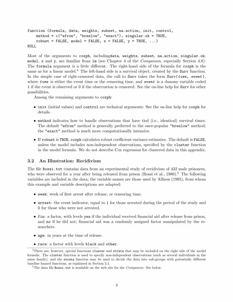
The summary method for Cox models produces a more complete report:

> summary(mod.allison)

Call:coxph(formula = Surv(week, arrest) ~ fin + age + race + wexp +

mar + paro + prio, data = Rossi)

n= 432, number of events= 114

coef exp(coef) se(coef) z Pr(>|z|)finyes -0.3794 0.6843 0.1914 -1.98 0.0474age -0.0574 0.9442 0.0220 -2.61 0.0090raceother -0.3139 0.7306 0.3080 -1.02 0.3081wexpyes -0.1498 0.8609 0.2122 -0.71 0.4803marnot married 0.4337 1.5430 0.3819 1.14 0.2561paroyes -0.0849 0.9186 0.1958 -0.43 0.6646prio 0.0915 1.0958 0.0286 3.19 0.0014

exp(coef) exp(-coef) lower .95 upper .95finyes 0.684 1.461 0.470 0.996age 0.944 1.059 0.904 0.986raceother 0.731 1.369 0.399 1.336wexpyes 0.861 1.162 0.568 1.305marnot married 1.543 0.648 0.730 3.261paroyes 0.919 1.089 0.626 1.348prio 1.096 0.913 1.036 1.159

Rsquare= 0.074 (max possible= 0.956 )Likelihood ratio test= 33.3 on 7 df, p=0.0000236Wald test = 32.1 on 7 df, p=0.0000387Score (logrank) test = 33.5 on 7 df, p=0.0000211

� The column marked z in the output records the ratio of each regression coefficient to itsstandard error, a Wald statistic which is asymptotically standard normal under the hypothesisthat the corresponding β is 0. The covariates age and prio (prior convictions) have highlystatistically significant coefficients, while the coefficient for fin (financial aid—the focus ofthe study) is marginally significant.

� The exponentiated coefficients in the second column of the first panel (and in the first columnof the second panel) of the output are interpretable as multiplicative effects on the hazard.

6

0 10 20 30 40 50

0.70

0.75

0.80

0.85

0.90

0.95

1.00

Weeks

Pro

port

ion

Not

Rea

rres

ted

Figure 1: Estimated survival function S(t) for the Cox regression of time to rearrest on severalpredictors. The broken lines show a point-wise 95-percent confidence envelope around the survivalfunction.

Thus, for example, holding the other covariates constant, an additional year of age reducesthe weekly hazard of rearrest by a factor of eb2 = 0.944 on average—that is, by 5.6 percent.Similarly, each prior conviction increases the hazard by a factor of 1.096, or 9.6 percent.

� The likelihood-ratio, Wald, and score chi-square statistics at the bottom of the output areasymptotically equivalent tests of the omnibus null hypothesis that all of the βs are 0. Inthis instance, the test statistics are in close agreement, and the omnibus null hypothesis issoundly rejected.

Having fit a Cox model to the data, it is often of interest to examine the estimated distribution ofsurvival times. The survfit function estimates S(t), by default at the mean values of the covariates.The plot method for objects returned by survfit graphs the estimated surivival function, alongwith a point-wise 95-percent confidence band. For example, for the model just fit to the recidivismdata:

> plot(survfit(mod.allison), ylim=c(0.7, 1), xlab="Weeks",

+ ylab="Proportion Not Rearrested")

This command produces Figure 1. The limits for the vertical axis, set by ylim=c(0.7, 1), wereselected after examining an initial plot.

Even more cogently, we may wish to display how estimated survival depends upon the valueof a covariate. Because the principal purpose of the recidivism study was to assess the impact offinancial aid on rearrest, we focus on this covariate. We construct a new data frame with two rows,one for each value of fin; the other covariates are fixed to their average values. For a dummycovariate, such as the contrast associated with race, the average value is the proportion coded 1 inthe data set—in the case of race, the proportion of non-blacks (cf., the discussion of effect displaysin Section 4.4.3 of the text). This data frame is passed to survfit via the newdata argument:

7

0 10 20 30 40 50

0.6

0.7

0.8

0.9

1.0

Weeks

Pro

port

ion

Not

Rea

rres

ted

fin = nofin = yes

Figure 2: Estimated survival functions for those receiving (fin = yes) and not receiving (fin =no) financial aid. Other covariates are fixed at their average values. Each estimate is accompaniedby a point-wise 95-percent confidence envelope.

> Rossi.fin <- with(Rossi, data.frame(fin=c(0, 1),

+ age=rep(mean(age), 2), race=rep(mean(race == "other"), 2),

+ wexp=rep(mean(wexp == "yes"), 2), mar=rep(mean(mar == "not married"), 2),

+ paro=rep(mean(paro == "yes"), 2), prio=rep(mean(prio), 2)))

> plot(survfit(mod.allison, newdata=Rossi.fin), conf.int=TRUE,

+ lty=c(1, 2), ylim=c(0.6, 1), xlab="Weeks",

+ ylab="Proportion Not Rearrested")

> legend("bottomleft", legend=c("fin = no", "fin = yes"), lty=c(1 ,2), inset=0.02)

Warning messages:1: In model.frame.default(Terms2, newdata, xlev = object$xlevels) :variable 'fin' is not a factor

2: In model.frame.default(Terms2, newdata, xlev = object$xlevels) :variable 'race' is not a factor

3: In model.frame.default(Terms2, newdata, xlev = object$xlevels) :variable 'wexp' is not a factor

4: In model.frame.default(Terms2, newdata, xlev = object$xlevels) :variable 'mar' is not a factor

5: In model.frame.default(Terms2, newdata, xlev = object$xlevels) :variable 'paro' is not a factor

The survfit command generates warnings because we supplied numerical values for factors (e.g.,the proportion of non-blacks for the factor race), but the computation is performed correctly. Wespecified two additional arguments to plot: lty=c(1, 2) indicates that the survival function forthe first group (i.e., for fin = no) will be plotted with a solid line, while that for the second group(fin = yes) will be plotted with a broken line; conf.int=TRUE requests that confidence envelopes

8

be drawn around each estimated survival function (which is not the default when more than onesurvival function is plotted). We used the legend function to place a legend on the plot.7 Theresulting graph, which appears in Figure 2, shows the higher estimated “survival” of those receivingfinancial aid, but the two confidence envelopes overlap substantially, even after 52 weeks.

4 Time-Dependent Covariates

The coxph function handles time-dependent covariates by requiring that each time period for anindividual appear as a separate observation—that is, as a separate row (or record) in the data set.Consider, for example, the Rossi data frame, and imagine that we want to treat weekly employmentas a time-dependent predictor of time to rearrest. As is often the case, however, the data for eachindividual appears as a single row, with the weekly employment indicators as 52 columns in thedata frame, with names emp1 through emp52; for example, for the first person in the study:

> Rossi[1, ]

week arrest fin age race wexp mar paro prio educ emp1 emp2 emp3 emp41 20 1 no 27 black no not married yes 3 3 no no no noemp5 emp6 emp7 emp8 emp9 emp10 emp11 emp12 emp13 emp14 emp15 emp16 emp17

1 no no no no no no no no no no no no noemp18 emp19 emp20 emp21 emp22 emp23 emp24 emp25 emp26 emp27 emp28 emp29 emp30

1 no no no <NA> <NA> <NA> <NA> <NA> <NA> <NA> <NA> <NA> <NA>emp31 emp32 emp33 emp34 emp35 emp36 emp37 emp38 emp39 emp40 emp41 emp42 emp43

1 <NA> <NA> <NA> <NA> <NA> <NA> <NA> <NA> <NA> <NA> <NA> <NA> <NA>emp44 emp45 emp46 emp47 emp48 emp49 emp50 emp51 emp52

1 <NA> <NA> <NA> <NA> <NA> <NA> <NA> <NA> <NA>

The employment indicators are missing after week 20, when individual 1 was rearrested.To put the data in the requisite form, we need one row for each non-missing period of observation.

To perform this task, we have written a function named unfold; the function is included with thescript file for this appendix, and takes the following arguments:8

� data: A data frame to be “unfolded” from “wide” to “long” format.

� time: The column number or quoted name of the event/censoring-time variable in data.

� event: The quoted name of the event/censoring indicator variable in data.

� cov: A vector giving the column numbers of the time-dependent covariate in data, or a listof vectors if there is more than one time-dependent covariate.

� cov.names: A character string or character vector giving the name(s) to be assigned to thetime-dependent covariate(s) in the output data set.

7The plot method for survfit objects can also draw a legend on the plot, but separate use of the legend functionprovides greater flexibility. Legends, line types, and other aspects of constructing graphs in R are described in Chapter7 of the Companion.

8This is a slightly simplified version of the unfold function in the RcmdrPlugin.survival package, which addssurvival-analysis capabilities to the R Commander graphical user interface to R (described in Section 1.5 of theCompanion). The Rossi data set is also included in the RcmdrPlugin.survival package.

9

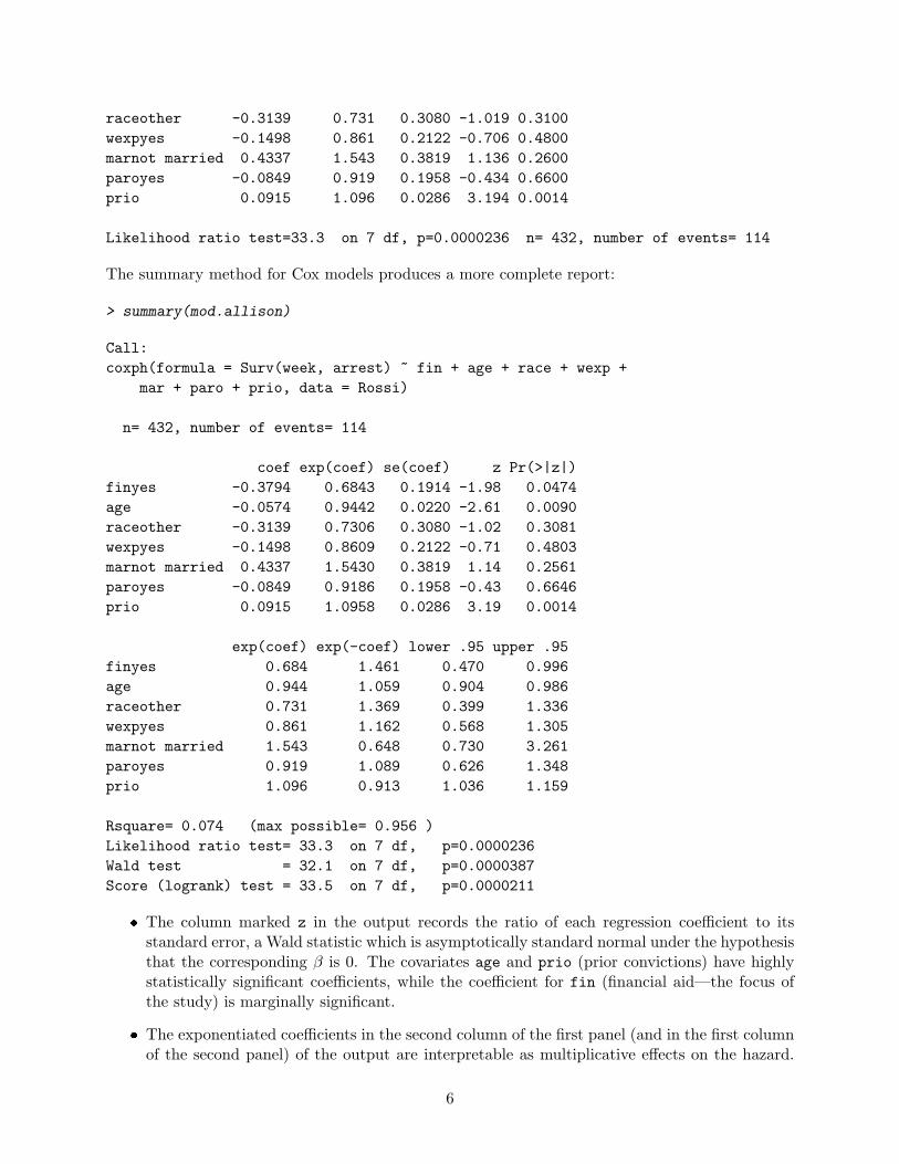
� suffix: The suffix to be attached to the name of the time-to-event variable in the outputdata set; defaults to ".time".

� cov.times: The observation times for the covariate values, including the start time. Thisargument can take several forms:

– The default is the vector of integers from 0 to the number of covariate values (i.e.,containing one more entry—the initial time of observation—than the length of eachvector in cov).

– An arbitrary numerical vector with one more entry than the length of each vector incov.

– The columns in the input data set that give the (potentially different) covariate obser-vation times for each individual. There should be one more column than the length ofeach vector in cov.

� common.times: A logical value indicating whether the times of observation are the same forall individuals; defaults to TRUE.

� lag: Number of observation periods to lag each value of the time-dependent covariate(s);defaults to 0. The use of lag is described later in this section.

Thus, to unfold the Rossi data, we enter:

> Rossi.2 <- unfold(Rossi, time="week",

+ event="arrest", cov=11:62, cov.names="employed")

> Rossi.2[1:50, ]

start stop arrest.time week arrest fin age race wexp mar paro prio educ employed1.1 0 1 0 20 1 no 27 black no not married yes 3 3 no1.2 1 2 0 20 1 no 27 black no not married yes 3 3 no. . .1.19 18 19 0 20 1 no 27 black no not married yes 3 3 no1.20 19 20 1 20 1 no 27 black no not married yes 3 3 no2.1 0 1 0 17 1 no 18 black no not married yes 8 4 no2.2 1 2 0 17 1 no 18 black no not married yes 8 4 no. . .2.16 15 16 0 17 1 no 18 black no not married yes 8 4 no2.17 16 17 1 17 1 no 18 black no not married yes 8 4 no3.1 0 1 0 25 1 no 19 other yes not married yes 13 3 no3.2 1 2 0 25 1 no 19 other yes not married yes 13 3 no. . .3.13 12 13 0 25 1 no 19 other yes not married yes 13 3 no

Once the data set is constructed, it is simple to use coxph to fit a model with time-dependentcovariates. The right-hand-side of the model is essentially the same as before, but both the startand end times of each interval are specified in the call to Surv, in the form Surv(start, stop,event ). Here, event is the time-dependent version of the event indicator variable, equal to 1 onlyin the time-period during which the event occurs. For the example:

10

> mod.allison.2 <- coxph(Surv(start, stop, arrest.time) ~

+ fin + age + race + wexp + mar + paro + prio + employed,

+ data=Rossi.2)

> summary(mod.allison.2)

Call:coxph(formula = Surv(start, stop, arrest.time) ~ fin + age +

race + wexp + mar + paro + prio + employed, data = Rossi.2)

n= 19809, number of events= 114

coef exp(coef) se(coef) z Pr(>|z|)finyes -0.3567 0.7000 0.1911 -1.87 0.0620age -0.0463 0.9547 0.0217 -2.13 0.0330raceother -0.3387 0.7127 0.3096 -1.09 0.2740wexpyes -0.0256 0.9748 0.2114 -0.12 0.9038marnot married 0.2937 1.3414 0.3830 0.77 0.4431paroyes -0.0642 0.9378 0.1947 -0.33 0.7416prio 0.0851 1.0889 0.0290 2.94 0.0033employedyes -1.3283 0.2649 0.2507 -5.30 1.2e-07

exp(coef) exp(-coef) lower .95 upper .95finyes 0.700 1.429 0.481 1.018age 0.955 1.047 0.915 0.996raceother 0.713 1.403 0.388 1.308wexpyes 0.975 1.026 0.644 1.475marnot married 1.341 0.745 0.633 2.842paroyes 0.938 1.066 0.640 1.374prio 1.089 0.918 1.029 1.152employedyes 0.265 3.775 0.162 0.433

Rsquare= 0.003 (max possible= 0.066 )Likelihood ratio test= 68.7 on 8 df, p=9.11e-12Wald test = 56.1 on 8 df, p=2.63e-09Score (logrank) test = 64.5 on 8 df, p=6.1e-11

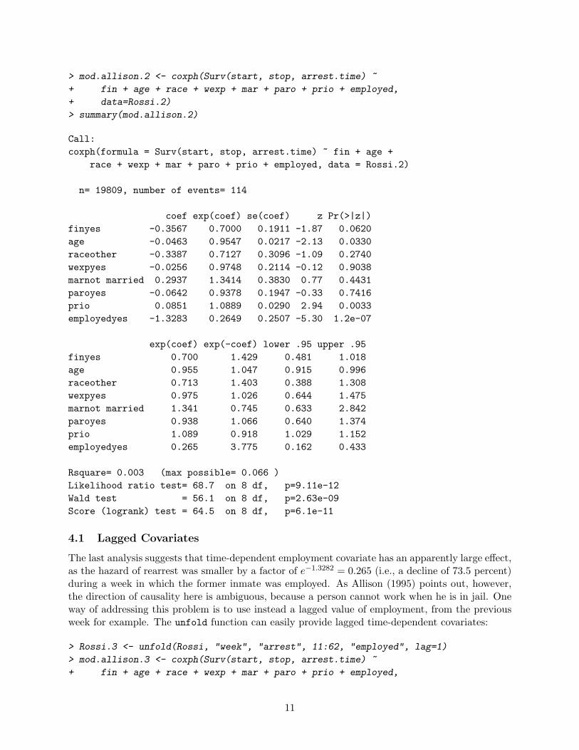
4.1 Lagged Covariates

The last analysis suggests that time-dependent employment covariate has an apparently large effect,as the hazard of rearrest was smaller by a factor of e−1.3282 = 0.265 (i.e., a decline of 73.5 percent)during a week in which the former inmate was employed. As Allison (1995) points out, however,the direction of causality here is ambiguous, because a person cannot work when he is in jail. Oneway of addressing this problem is to use instead a lagged value of employment, from the previousweek for example. The unfold function can easily provide lagged time-dependent covariates:

> Rossi.3 <- unfold(Rossi, "week", "arrest", 11:62, "employed", lag=1)

> mod.allison.3 <- coxph(Surv(start, stop, arrest.time) ~

+ fin + age + race + wexp + mar + paro + prio + employed,

11

+ data=Rossi.3)

> summary(mod.allison.3)

Call:coxph(formula = Surv(start, stop, arrest.time) ~ fin + age +

race + wexp + mar + paro + prio + employed, data = Rossi.3)

n= 19377, number of events= 113

coef exp(coef) se(coef) z Pr(>|z|)finyes -0.3513 0.7038 0.1918 -1.83 0.06703age -0.0498 0.9514 0.0219 -2.27 0.02297raceother -0.3215 0.7251 0.3091 -1.04 0.29837wexpyes -0.0476 0.9535 0.2132 -0.22 0.82321marnot married 0.3448 1.4116 0.3832 0.90 0.36831paroyes -0.0471 0.9540 0.1963 -0.24 0.81038prio 0.0920 1.0964 0.0288 3.19 0.00140employedyes -0.7869 0.4553 0.2181 -3.61 0.00031

exp(coef) exp(-coef) lower .95 upper .95finyes 0.704 1.421 0.483 1.025age 0.951 1.051 0.911 0.993raceother 0.725 1.379 0.396 1.329wexpyes 0.953 1.049 0.628 1.448marnot married 1.412 0.708 0.666 2.992paroyes 0.954 1.048 0.649 1.402prio 1.096 0.912 1.036 1.160employedyes 0.455 2.197 0.297 0.698

Rsquare= 0.002 (max possible= 0.067 )Likelihood ratio test= 47.2 on 8 df, p=1.43e-07Wald test = 43.4 on 8 df, p=7.48e-07Score (logrank) test = 46.4 on 8 df, p=1.99e-07

The coefficient for the now-lagged employment indicator is still highly statistically significant, butthe estimated effect of employment, though still substantial, is much smaller than before: e−0.7869 =0.455 (or a decrease of 54.5 percent).

5 Model Diagnostics

As is the case for a linear or generalized linear model (see Chapter 6 of the Companion), it isdesirable to determine whether a fitted Cox regression model adequately describes the data. Wewill briefly consider three kinds of diagnostics: for violation of the assumption of proportionalhazards; for influential data; and for nonlinearity in the relationship between the log hazard and thecovariates. All of these diagnostics use the residuals method for coxph objects, which calculatesseveral kinds of residuals, along with some quantities that are not normally thought of as residuals.Details are in Therneau (1999).

12

5.1 Checking Proportional Hazards

Tests and graphical diagnostics for proportional hazards may be based on the scaled Schoenfeldresiduals; these can be obtained directly as residuals(model, "scaledsch"), where model is acoxph model object. The matrix returned by residuals has one column for each covariate inthe model. More conveniently, the cox.zph function calculates tests of the proportional-hazardsassumption for each covariate, by correlating the corresponding set of scaled Schoenfeld residualswith a suitable transformation of time [the default is based on the Kaplan-Meier estimate of thesurvival function, K(t)].

We will illustrate these tests with a scaled-down version of the Cox regression model fit to therecidivism data in Section 3.2, eliminating the covariates whose coefficients were not statisticallysignificant:9

> mod.allison.4 <- coxph(Surv(week, arrest) ~ fin + age + prio,

+ data=Rossi)

> mod.allison.4

Call:coxph(formula = Surv(week, arrest) ~ fin + age + prio, data = Rossi)

coef exp(coef) se(coef) z pfinyes -0.3470 0.707 0.1902 -1.82 0.06800age -0.0671 0.935 0.0209 -3.22 0.00130prio 0.0969 1.102 0.0273 3.56 0.00038

Likelihood ratio test=29.1 on 3 df, p=2.19e-06 n= 432, number of events= 114

The coefficient for financial aid, which is the focus of the study, now has a two-sided p-value greaterthan .05; a one-sided test is appropriate here, however, because we expect the coefficient to benegative, so there is still marginal evidence for the effect of this covariate on the time of rearrest.

As mentioned, tests for the proportional-hazards assumption are obtained from cox.zph, whichcomputes a test for each covariate, along with a global test for the model as a whole:

> cox.zph(mod.allison.4)

rho chisq pfinyes -0.00657 0.00507 0.9433age -0.20976 6.54147 0.0105prio -0.08004 0.77288 0.3793GLOBAL NA 7.13046 0.0679

There is, therefore, strong evidence of non-proportional hazards for age, while the global test (on3 degrees of freedom) is not quite statistically significant. These tests are sensitive to linear trendsin the hazard.

Plotting the object returned by cox.zph produces graphs of the scaled Schoenfeld residualsagainst transformed time (see Figure 3):

9It is possible that a covariate that is not statistically significant when its effect is, in essence, averaged over timenevertheless has a statistically significant interaction with time, which manifests itself as nonproportional hazards.We leave it to the reader to check for this possibility using the model fit originally to the recidivism data.

13

Time

Bet

a(t)

for

finye

s

7.9 14 20 25 32 37 44 49

−2

−1

01

2

●

●

●

●●●

●

●

●

●

●

●●●

●

●

●

●●

●●●

●

●●

●

●

●●●●●

●●

●

●

●●●●

●●

●

●

●●

●

●

●

●

●

●●●

●

●●●

●

●

●●

●

●●

●

●●●●

●

●●●

●

●

●

●

●●

●●

●●●

●●

●●●●

●●●

●●●●

● ●●

●

●

●

●

●● ●●

●●●●

●

Time

Bet

a(t)

for

age

7.9 14 20 25 32 37 44 49

−0.

40.

00.

20.

40.

60.

81.

0

●

●

●

●●●●

●

●

●

●

●

●

●

●

●

●

●

●

●●

●●

●

●

●

●

●

●

●

●

●

●

●

●

●

●

●

●

●

●

●

●

●

●

●

●

●

●●

●

●

●

●

●

●●

●

●

●

●●●

●

●

●

●●●●

●

●

●

●●

●

●

●

●

●

●

●●●

●

●

●

●

●

●

●●●●

●

●

●

●

●

●

●

●

●

●

●

●●

●●

●●

●

●

●

Time

Bet

a(t)

for

prio

7.9 14 20 25 32 37 44 49

0.0

0.5

1.0

●

●●

●

●

●

●●

●

●

●●

●

●

●

●

●

●

●

●

●

●

●

●

●

●

●

●●

●

●●●●

●

●

●

●●●●

●

●

●

●

●●

●

●

●

●

●

●●

●

●

●

●●

●

●

●

●

●

●

●

●

●

●

●

●

●●

●

●

●

●

●

●

●●

●

●

●

●

●

●

●

●●

●

●

●

●●

●

●

●

●

●

●

●●

●●

●

●

●

●

●

●

●

●

●

Figure 3: Plots of scaled Schoenfeld residuals against transformed time for each covariate in a modelfit to the recidivism data. The solid line is a smoothing spline fit to the plot, with the broken linesrepresenting a ± 2-standard-error band around the fit.

> par(mfrow=c(2, 2))

> plot(cox.zph(mod.allison.4))

Interpretation of these graphs is greatly facilitated by smoothing, for which purpose cox.zph usesa smoothing spline, shown on each graph by a solid line; the broken lines represent ± 2-standard-error envelopes around the fit. Systematic departures from a horizontal line are indicative ofnon-proportional hazards. The assumption of proportional hazards appears to be supported forthe covariates fin (which is, recall, a two-level factor, accounting for the two bands in the graph)and prio, but there appears to be a trend in the plot for age, with the age effect declining withtime; this effect was also detected in the test reported above.

One way of accommodating non-proportional hazards is to build interactions between covariatesand time into the Cox regression model; such interactions are themselves time-dependent covariates.For example, based on the diagnostics just examined, it seems reasonable to consider a linear

14

interaction of time and age; using the previously constructed Rossi.2 data frame:

> mod.allison.5 <- coxph(Surv(start, stop, arrest.time) ~

+ fin + age + age:stop + prio,

+ data=Rossi.2)

> mod.allison.5

Call:coxph(formula = Surv(start, stop, arrest.time) ~ fin + age +

age:stop + prio, data = Rossi.2)

coef exp(coef) se(coef) z pfinyes -0.34856 0.706 0.19023 -1.832 0.06700age 0.03228 1.033 0.03943 0.819 0.41000prio 0.09818 1.103 0.02726 3.602 0.00032age:stop -0.00383 0.996 0.00147 -2.612 0.00900

Likelihood ratio test=36 on 4 df, p=2.85e-07 n= 19809, number of events= 114

As expected, the coefficient for the interaction is negative and highly statistically significant: Theeffect of age declines with time.10 The model does not require a “main-effect” term for stop (i.e.,time); such a term would be redundant, because the time effect is the baseline hazard.

An alternative to incorporating an interaction in the model is to divide the data into strata basedon the value of one or more covariates. Each stratum is permitted to have a different baseline hazardfunction, while the coefficients of the remaining covariates are assumed to be constant across strata.An advantage of this approach is that we do not have to assume a particular form of interactionbetween the stratifying covariates and time. A disadvantage is the resulting inability to examinethe effects of the stratifying covariates. Stratification is most natural when a covariate takes ononly a few distinct values, and when the effect of the stratifying variable is not of direct interest.In our example, age takes on many different values, but we can create categories by arbitrarilydissecting the variable into class intervals. After examining the distribution of age, we decided todefine four intervals: 19 or younger; 20 to 25; 26 to 30; and 31 or older. We use the recode functionin the car package to categorize age:11

> library(car)

> Rossi$age.cat <- recode(Rossi$age, " lo:19=1; 20:25=2; 26:30=3; 31:hi=4 ")

> xtabs(~ age.cat, data=Rossi)

age.cat1 2 3 466 236 66 64

Most of the individuals in the data set are in the second age category, 20 to 25, but because this isa reasonably narrow range of ages, we did not feel the need to sub-divide the category.

10That is, initially, age has a positive partial effect on the hazard (given by the age coefficient, 0.032), but thiseffect gets progressively smaller with time (at the rate −0.0038 per week), becoming negative after about 10 weeks.

11An alternative is to use the standard R function cut: cut(Rossi$age, c(0, 19, 25, 30, Inf)). See Chapter2 of the Companion.

15

A stratified Cox regression model is fit by including a call to the strata function on the right-hand side of the model formula. The arguments to this function are one or more stratifying variables;if there is more than one such variable, then the strata are formed from their cross-classification.In the current illustration, there is just one stratifying variable:

> mod.allison.6 <- coxph(Surv(week, arrest) ~

+ fin + prio + strata(age.cat), data=Rossi)

> mod.allison.6

Call:coxph(formula = Surv(week, arrest) ~ fin + prio + strata(age.cat),

data = Rossi)

coef exp(coef) se(coef) z pfinyes -0.341 0.711 0.190 -1.79 0.0730prio 0.094 1.099 0.027 3.48 0.0005

Likelihood ratio test=13.4 on 2 df, p=0.00122 n= 432, number of events= 114

> cox.zph(mod.allison.6)

rho chisq pfinyes -0.0183 0.0392 0.843prio -0.0771 0.6859 0.408GLOBAL NA 0.7299 0.694

There is no evidence of non-proportional hazards for the remaining covariates.

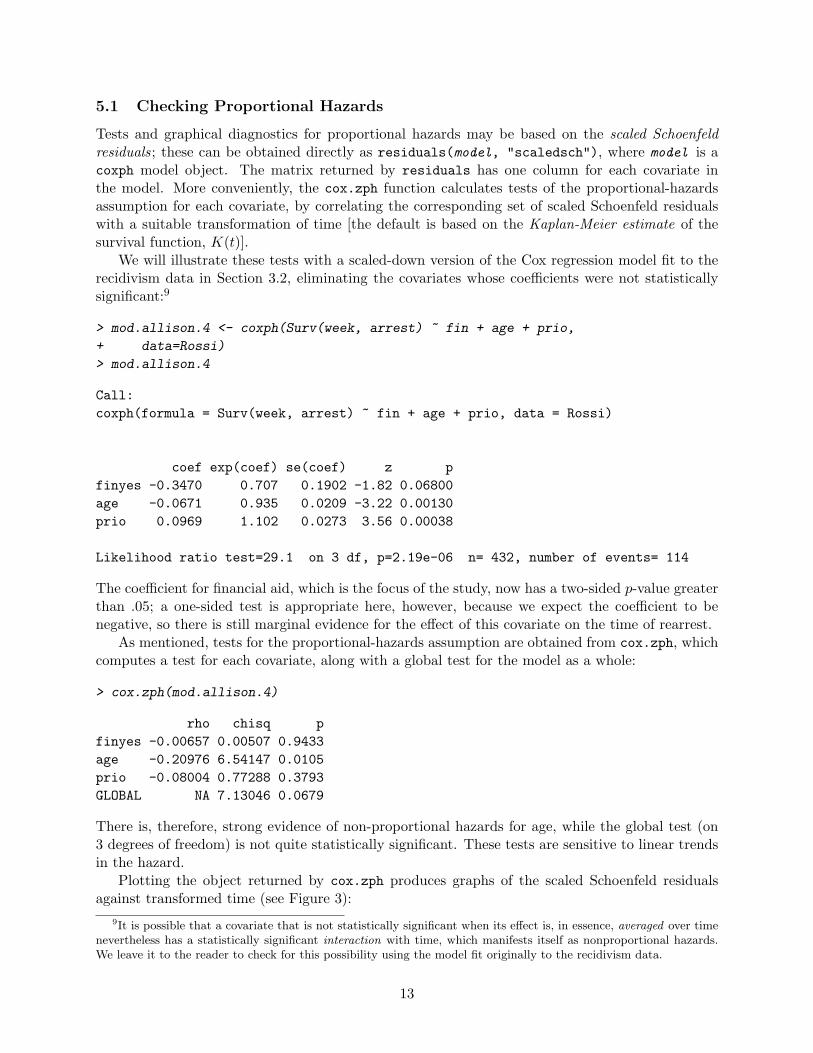
5.2 Influential Observations

Specifying the argument type=dfbeta to residuals produces a matrix of estimated changes in theregression coefficients upon deleting each observation in turn; likewise, type=dfbetas produces theestimated changes in the coefficients divided by their standard errors (cf., Sections 6.3 and 6.6 ofthe Companion for similar diagnostics for linear and generalized linear models).

For example, for the model regressing time to rearrest on financial aid, age, and number of prioroffenses:

> dfbeta <- residuals(mod.allison.4, type="dfbeta")

> par(mfrow=c(2, 2))

> for (j in 1:3) {

+ plot(dfbeta[, j], ylab=names(coef(mod.allison.4))[j])

+ abline(h=0, lty=2)

+ }

The index plots produced by these commands appear in Figure 4. Comparing the magnitudes ofthe largest dfbeta values to the regression coefficients suggests that none of the observations isterribly influential individually, even though some of the dfbeta values for age are large comparedwith the others.12

12As an exercise, the reader may wish to identify these observations and, in particular, examine their ages.

16

●

●

●

●

●

●

●

●

●

●

●

●

●

●

●

●

●

●

●

●

●

●

●

●●

●

●

●

●●

●●

●

●●

●

●

●

●

●

●

●

●

●

●●

●

●

●

●●

●

●

●

●●●●

●

●

●

●

●●

●

●●●

●

●

●

●

●

●●

●

●

●

●

●●

●

●

●

●

●

●

●

●●

●

●

●

●

●

●

●●

●●

●

●

●

●

●

●

●●

●●

●

●

●

●

●●●

●

●

●

●

●

●

●

●

●

●

●

●

●

●

●

●

●

●●●

●

●

●

●

●

●

●

●

●

●

●

●

●

●

●

●

●

●

●

●

●●

●

●

●

●●●

●

●

●

●

●

●

●

●

●

●

●

●

●●

●

●

●

●

●

●

●

●

●

●

●●

●●●

●

●●

●●●●

●

●

●●

●●

●

●

●

●

●

●●

●

●

●

●

●●

●

●

●

●●

●

●

●

●

●

●

●

●

●

●

●

●●●●●

●

●●

●

●

●

●●

●

●●

●●

●●

●

●

●

●

●

●

●

●

●

●

●

●

●

●

●

●●

●

●

●●●●

●●

●

●●

●

●

●

●●

●

●

●

●

●

●

●

●●●

●

●●

●

●

●

●

●

●

●

●●

●

●

●

●●●

●

●

●

●

●

●

●

●

●●

●

●

●

●

●

●

●

●

●

●

●

●

●

●

●

●

●

●

●

●

●

●

●

●

●

●

●●●

●

●

●

●

●

●

●

●●

●

●

●

●

●

●

●

●

●

●●●

●

●

●

●

●

●

●●

●●

●

●

●●

●

●

●

●

●

●

●●

●

●

●

●

●●

●

●

●●●

●

●

●

●

●

●

●

●

●

●●

●●

●

●

●

●

●

●

●

●

●

0 100 200 300 400

−0.

02−

0.01

0.00

0.01

0.02

Index

finye

s

●

●

●

●

●

●

●

●●●

●

●

●

●●●●

●

●

●●●

●

●

●●

●

●●

●●●

●●●

●

●

●

●

●●

●●●●●●●

●●●

●

●●●●●●

●

●●

●●

●

●●

●●

●

●

●

●

●

●

●

●

●

●

●

●

●

●

●●

●

●●●●●

●

●●●●●

●●

●●

●

●

●

●

●

●

●

●●

●

●

●●

●●●●

●

●

●●

●

●●●●●

●●●●

●

●●●●●

●

●●●

●●

●

●

●●

●●

●

●●

●

●●

●●

●●●

●●

●●●

●

●

●

●

●●

●

●

●●

●

●●●●

●

●●

●

●

●●

●●●

●●●●

●

●●●

●●●●●

●

●

●

●

●

●

●●

●●●●●●●●●●

●●●●

●

●

●

●

●

●

●

●●

●

●

●

●●

●

●

●

●●

●●

●●●

●

●●●●

●●●●

●

●●

●●

●

●

●

●●●●

●

●●

●

●●●●●

●

●●●●

●

●

●

●●●

●

●●

●

●●●●●

●

●●

●

●

●●●

●

●

●●

●

●

●

●●

●

●

●

●

●

●

●

●

●

●●

●

●

●

●●

●●

●

●

●

●

●

●●●

●

●●●●

●●

●

●

●

●

●●●●●●

●●

●●

●●●●●●

●

●●●

●●●●

●●●

●●

●

●●●●●

●

●

●●

●

●●

●

●

●●

●

●●●●●

●●●●●●

●●●

●

●●

●

●

●●

●●

●

●

●●●

●●

●

●

0 100 200 300 400

−0.

002

0.00

20.

006

Index

age

●

●

●

●●●

●

●

●

●

●●●●●●

●

●

●

●●●

●

●●●●●●

●

●●●●●

●●

●●●

●

●

●

●●●

●

●●●●●●

●

●●●●●

●

●

●

●

●

●

●●●●●●

●

●●●●●●●

●

●●

●

●

●

●●●●●●

●●●●●●●●●

●●

●

●

●

●

●●●●

●

●●●●●●●

●

●

●

●

●

●

●●●

●

●●

●●●●●●●●

●

●

●

●

●

●

●●●

●

●

●

●●

●

●

●

●

●●●

●●

●

●

●●●

●

●●●●

●

●

●

●

●

●

●

●

●

●

●

●●

●●●●

●

●●●●●●●●●●●●

●

●

●

●

●●●●

●

●●●●●

●

●●●●●●●●●

●

●●●

●

●

●

●

●

●●●●●●●

●

●●●

●●

●●

●

●●●

●

●●●●

●

●●●

●

●

●●●●

●

●

●

●●

●●●●●●●●

●●●●

●

●●●●

●

●

●

●

●●●●●●

●●

●

●●●●●●●●

●●

●

●

●

●

●●

●

●

●

●●

●

●●

●●

●

●

●

●

●

●

●

●●

●

●●●

●

●●●

●

●●

●

●

●●●●●●●

●

●●

●

●

●●

●●●●

●

●●

●

●

●●●●●●

●●

●

●●●●

●●

●

●●

●

●

●

●

●

●●

●

●●

●

●●●●●●●

●

●●●

●

●

●

●●

●●

●●

●

●

●

●

●

●●●●

0 100 200 300 400

−0.

005

0.00

00.

005

Index

prio

Figure 4: Index plots of dfbeta for the Cox regression of time to rearrest on fin, age, and prio.

17

5.3 Nonlinearity

Nonlinearity—that is, an incorrectly specified functional form in the parametric part of the model—is a potential problem in Cox regression as it is in linear and generalized linear models (see Sections6.4 and 6.6 of the Companion). The martingale residuals may be plotted against covariates todetect nonlinearity, and may also be used to form component-plus-residual (or partial-residual)plots, again in the manner of linear and generalized linear models.

For the regression of time to rearrest on financial aid, age, and number of prior arrests, let usexamine plots of martingale residuals and partial residuals against the last two of these covariates;nonlinearity is not an issue for financial aid, because this covariate is dichotomous:

> par(mfrow=c(2, 2))

> res <- residuals(mod.allison.4, type="martingale")

> X <- as.matrix(Rossi[, c("age", "prio")]) # matrix of covariates

> par(mfrow=c(2, 2))

> for (j in 1:2) { # residual plots

+ plot(X[, j], res, xlab=c("age", "prio")[j], ylab="residuals")

+ abline(h=0, lty=2)

+ lines(lowess(X[, j], res, iter=0))

+ }

> b <- coef(mod.allison.4)[c(2,3)] # regression coefficients

> for (j in 1:2) { # component-plus-residual plots

+ plot(X[, j], b[j]*X[, j] + res, xlab=c("age", "prio")[j],

+ ylab="component+residual")

+ abline(lm(b[j]*X[, j] + res ~ X[, j]), lty=2)

+ lines(lowess(X[, j], b[j]*X[, j] + res, iter=0))

+ }

The resulting residual and component-plus-residual plots appear in Figure 5. As in the plots ofSchoenfeld residuals, smoothing these plots is also important to their interpretation; The smoothsin Figure 5 are produced by local linear regression using the lowess function; setting iter=0 selectsa non-robust smooth, which is generally advisable in plots that may be banded. Nonlinearity, itappears, is slight here.

6 Complementary Reading and References

There are many texts on survival analysis: Cox and Oakes (1984) is a classic (if now slightly dated)source, coauthored by the developer of the Cox model. As mentioned, the running example in thisappendix is adapted from Allison (1995), who presents a highly readable introduction to survivalanalysis based on the SAS statistical package, but nevertheless of general interest. Allison (1984)is a briefer treatment of the subject by the same author. Another widely read and wide-rangingtext on survival analysis is Hosmer and Lemeshow (1999). The book by Therneau and Grambsch(2000) is also worthy of mention here; Therneau is the author of the survival package for R, andthe text, which focusses on relatively advanced topics, develops examples using both the survivalpackage and SAS. Extensive documentation for the survival package may be found in Therneau(1999); although the survival package has continued to evolve since 1999, this technical reportremains a useful source of information about it.

18

●

●

●

●

●

●

●

●

●

●

●

●

●

●

● ●

●

●

●

●

●

●

●

●●

●

●

●

●

●

●●

●

● ●

●

●

●

●

● ●●

●

●●

●

●

●

●●●

●

●

●

● ●●

●●

●

●

●

●

●

●

●● ●

●

●

●

●

●●

●

●

●

●

●

●

●

●

●●

●

●

●

●

●●

●

●●

●

●

●

●●

●●

●●

●

●

●

●

●

●

●●

●

●

●

●

●● ●

●

●

● ●

●

●

●

●

●

●

●

●

●

●

●●

●

●●

●

●

●

●

●

●

●

●

●

●●

●

●

●

●

●

●

●

●

●

●

●●

●

●

●

●●

●●

●

●

●

●

●

●

●

●

●

●

●

●●

●

●

●

●

●

●

●

●

●

●

●

●

●● ●

●

● ●●

● ●●

●

●

●●

●

●●

●

●

●

●

●●

●

●

●

●

●●

●

●

●

●●

●

●

●

●

●

●

●

●

●

●

●

●

●●●

●

●

● ●

● ●

●

●●

●

●●●

●

●● ●

●

●

●

●

●

●

●

●

●

●

●

●

●

●●

●

●

●

●● ●●

●●●

●●

●

●

●

●●

●

●

●

●

●

● ●●●●

●

● ●

●

●

● ●

●

●

●

●●●

●

●

●

●

●

●

●

●

●

●

●

●●

● ●

●

●

●

●

●

●

●

●

●

●

●

●

●

●

●

●

●

●●

●

●

●

●●●

●●

●●

●

●

●

●

●●

●

● ●

●

●●●

●

●

●

●

●

●

●

●●

●

●

●

●

●

●

●

●●

●

●

●●

●

●

●

●

●

●

●

●

●

●●

●

●●

●

●

● ●●

●

●

●●

●●

●

●●

●●

● ●

●

●

●

●

●

●

● ●●

20 25 30 35 40 45

−1.

0−

0.5

0.0

0.5

1.0

age

resi

dual

s

●

●

●

●

●

●

●

●

●

●

●

●

●

●

●●

●

●

●

●

●

●

●

●●

●

●

●

●

●

●●

●

● ●

●

●

●

●

● ●●

●

●●●

●

●

●●●

●

●

●

● ●●

●●

●

●

●

●

●

●

●● ●

●

●

●

●

●●

●

●

●

●

●

●

●

●

●●

●

●

●

●

●●

●

●●

●

●

●

●●

●●

●●

●

●

●

●

●

●

●●

●

●

●

●

●● ●

●

●

● ●

●

●

●

●

●

●

●

●

●

●

●●

●

●●

●

●

●

●

●

●

●

●

●

●●

●

●

●

●

●

●

●

●

●

●

●●

●

●

●

●●

●●

●

●

●

●

●

●

●

●

●

●

●

●●

●

●

●

●

●

●

●

●

●

●

●

●

●● ●

●

● ●●

● ●●

●

●

●●

●

●●

●

●

●

●

●●

●

●

●

●

●●

●

●

●

●●

●

●

●

●

●

●

●

●

●

●

●

●

●●●

●

●

●●

●●

●

●●

●

●● ●

●

●●●

●

●

●

●

●

●

●

●

●

●

●

●

●

●●

●

●

●

●● ●

●

●●

●

●●

●

●

●

●●

●

●

●

●

●

●● ●●●

●

● ●

●

●

●●

●

●

●

●●●

●

●

●

●

●

●

●

●

●

●

●

●●

●●

●

●

●

●

●

●

●

●

●

●

●

●

●

●

●

●

●

●●

●

●

●

●●●

●●

●●

●

●

●

●

●●

●

●●

●

●●●

●

●

●

●

●

●

●

●●

●

●

●

●

●

●

●

●●

●

●

●●

●

●

●

●

●

●

●

●

●

●●

●

● ●

●

●

● ●●

●

●

●●

●●

●

●●

●●

●●

●

●

●

●

●

●

● ●●

0 5 10 15−

1.0

−0.

50.

00.

51.

0

prio

resi

dual

s

●

●

●

●●

●

●

●

●

●

●

●

●

●

●

●●

●

●

●●

●

●

●

●●

●

●●

●

●

●

●

●●

●

●●

●

●

●

●

●

●

●

●

●

●

●

●

●

●

●

●

●

● ●

●

●

●

●

●●

●

●

●

●●

●

●●

●

●

●

●

●

●

●

●

●

●

●

●●

●

●

●

●

● ●

●

●●

●

●

●

●●

●●

●

●

●

●

●

●●

●●

●●

●●

●

●●

●

●●

●●

●

●

●

●

● ●●

●

●

●

●

●

●

●●●

●

●

●

●

●

●

●

●

●

●

●

●

●

●

●

●

●

●

●

●

●

●

●

●

●

●

●

●

●

●

●●

●

●

●

●

●

●

●

●

●

●

●

●

●

●

●

●

●●

●● ●

●●

●●

●

●

●●

●●●

●

●

●

●

●

●

●

●

●

●

●●●

●

●

●

●

●

●

●

●

●

●●

●

●

●

●

●

●

●

●

●

●

●

●

●●

●

●

●

● ●

●

●

●

●●

●

●●

●

●

●

●

●

●

●

●

●

●

●

●

●●

●

●

●

●

●

●●

●

●

●

●

●

●

●

●●

●

●

● ●●

●

●

●

●

●

●

●

●●

●●●

●

●●

●

●

●

●

●

●

●●

●

●

●

●

●●

●

●

●

●●

●

●

●

●

● ●

●

●

●

●

●

●

●

●

●

●

●●

●

●

●

●

●

●

●

●

●●

●

●

●

●

●

●

●

●

●

●

●

●

●

●

● ●

●

●●

●

●●●

●

●

●

●

●

●

●

●

●

●

●

● ●

●

●

●●

●

● ●

●

●

●

●

●

●●

●

●

●

●

●●

●

●

●

●

●

●

●●

●

●

●

●

●

●

●●

●●

●

●

●

●

●

●●

●

●

20 25 30 35 40 45

−3.

0−

2.5

−2.

0−

1.5

−1.

0−

0.5

age

com

pone

nt+

resi

dual

●

●

●

●●

●

●

● ●

●

●●

●

●

●

●

●

●

●

●

●●

●

●

●●

●

●

●

●

●

●●

●●

●

●●

●●

●

●

●

●●●

●

●

●

●● ●

●

●

●

●

●●

●

●

●

●

●

●

●

●

●●

●

●

●

●

●

●

●

●

●

●

●

● ●

●

●

●

●

●●

●

●●

●

●

●● ●

●

●●●

●

●●

●

●

●

●●

●●

● ●●

●

●

● ●

● ●

●

●

●

●

●

●

●●●

●

● ●

●

●●

●

● ● ●

●

●

●

●

●

●

●

●

●●

●

●

●

●

●

●

●

●

●

●●

●

●

●

●

●

● ●

● ●

●

●

●●

●

●

●

●●

●

●

●

●

●

●

●

●

●●

●

●

●

●

●●●●

●

●

●

●

●●

●

●

●

●●

●●

●

●

●

●●

●●●

●

● ●● ●

●

●●●

●

●

●●

●●

●

●

●

●

●

●

●●●

●

●

●

●●

●

●

●●

●

●

● ●

●

●●

●

● ●

●

●

●

●

●

●

● ●

● ●

●

●

●

●

●

●●●●●● ●

●

●

●●

●

●●

●●

●

●

●

●

●

●

●●

●●

●

●●

●

●

●●

●

●

●

●

●

●

●

● ●●

●

●

● ●

●

●

●

●●

●●

●

●

●

●

●

●

●

●

●

●

●

●

●●

●

●

●

●●

●

● ●

●

●

●

●●●●

●

●

●

●

●

●

●

●●

●

●

●

●

●●

●

●

●

●●●

●●

●

●

●

●

●●●

●

●

●

●

●●

●

●

●

●

●

●●

●

●●

●

●●

●

●

●

●●

●

●●●

●

●●●●

●●

●●

●

●

●

●

●

●●

●

●

0 5 10 15

−0.

50.

00.

51.

01.

52.

02.

5

prio

com

pone

nt+

resi

dual

Figure 5: Martingale-residual plots (top) and component-plus-residual plots (bottom) for the co-variates age and prio. The broken lines on the residual plots are at the vertical value 0, and on thecomponent-plus-residual plots are fit by linear least-squares; the solid lines are fit by local linearregression (lowess).

19

References

Allison, P. A. (1984). Event History Analysis: Regression for Longitudinal Data. Sage, NewburyPark CA.

Allison, P. D. (1995). Survival Analysis Using the SAS System: A Practical Guide. SAS Institute,Cary NC.

Cox, D. R. (1972). Regression models and life tables (with discussion). Journal of the RoyalStatistical Society, Series B, 34:187–220.

Cox, D. R. and Oakes, D. (1984). Analysis of Survival Data. Chapman and Hall, London.

Fox, J. and Weisberg, S. (2011). An R Companion to Applied Regression. Sage, Thousand Oaks,CA, second edition.

Hosmer, Jr., D. W. and Lemeshow, S. (1999). Applied Survival Analysis: Regression Modeling ofTime to Event Data. Wiley, New York.

Rossi, P. H., Berk, R. A., and Lenihan, K. J. (1980). Money, Work and Crime: Some ExperimentalResults. Academic Press, New York.

Therneau, T. M. (1999). A package for survival analysis in S. Technical report, Mayo Foundation,Rochester MN.

Therneau, T. M. and Grambsch, P. M. (2000). Modeling Surival Data: Extending the Cox Model.Springer, New York.

20