Covariate Model Building in Nonlinear Mixed Effects Models170387/FULLTEXT01.pdf · A population...

ACTAUNIVERSITATISUPSALIENSISUPPSALA2007

Digital Comprehensive Summaries of Uppsala Dissertationsfrom the Faculty of Pharmacy 59

Covariate Model Building inNonlinear Mixed Effects Models

JAKOB RIBBING

ISSN 1651-6192ISBN 978-91-554-6915-3urn:nbn:se:uu:diva-7923

We are drowning in information and starving for knowledge.

Rutherford D. Roger

Papers Discussed

Th is thesis is based on the following papers, which will be referred to in the text by their Roman numerals.

I Ribbing J and Jonsson EN. Power, Selection Bias and Predictive Per-formance of the Population Pharmacokinetic Covariate Model. Journal of Pharmacokinetics and Pharmacodynamics 2004;31(2):109-134.

Copyright Springer. Reproduced with permission

II Ribbing J, Nyberg J, Caster O and Jonsson EN. Th e Lasso – A Novel Method for Predictive Covariate Model Building in Nonlinear Mixed Eff ects Models. Accepted for publication in the Journal of Pharmacokinet-ics and Pharmacodynamics

Copyright Springer. Manuscript reproduced with permission.

III Ribbing J, Hooker AC and Jonsson EN. Non-Bayesian Knowledge Propagation using Model-Based Analysis of Data from Multiple Clini-cal Studies. Submitted

IV Ribbing J, Hamrén B, Svensson MK and Karlsson MO. A Model for Glucose, Insulin, Beta-Cell and HbA1c Dynamics in Subjects with Insulin Resistance and Patients with Type 2 Diabetes. In Manuscript

Contents

1. Introduction ........................................................................................111.1. Background ............................................................................................ 111.2. Nonlinear Mixed Eff ects Models ............................................................ 131.3. Th e Covariate Model .............................................................................. 15

1.3.1. What is a covariate? .......................................................................................... 151.3.2. What is a true covariate? ................................................................................... 161.3.3. Multiplicative and additive parameterisation .................................................... 161.3.4. Categorical covariates ....................................................................................... 171.3.5. Continuous covariates ...................................................................................... 181.3.6. Covariate transformation .................................................................................. 19

1.4. Software for Model Fitting ..................................................................... 191.5. Estimation Methods in NONMEM ....................................................... 20

1.5.1. Individual empirical bayes estimates and shrinkage ........................................... 211.6. Model Development and Selection ......................................................... 21

1.6.1. Stepwise selection ............................................................................................. 231.7. Th e Base Model ..................................................................................... 231.8. Selection of the Covariate Model ........................................................... 24

1.8.1. Covariate selection outside NONMEM ........................................................... 241.8.2. Covariate selection within NONMEM ............................................................ 26

1.9. Th e Lasso in Ordinary Multiple Regression............................................ 291.10. Model Validation and Evaluation ........................................................... 29

1.10.1. Cross-validation ............................................................................................... 301.11. Modelling of Type 2 Diabetes ................................................................ 32

2. Aims ...................................................................................................34

3. Methods ..............................................................................................353.1. Software ................................................................................................. 353.2. Analysed Data ........................................................................................ 35

3.2.1. Simulated data (Papers I-III) ............................................................................ 363.2.2. Real data (Papers II and IV) ............................................................................. 37

3.3. Development of the Lasso for Covariate Selection within NONMEM (Paper II) ............................................................................................... 37

3.4. Procedure for Analysis of nlme Models (Papers I-III) ............................. 383.5. Development of a Model for FPG and FI (Paper IV) .............................. 403.6. Adaptive Learning (Paper III) ................................................................ 423.7. Calculation of Power and Inclusion Rates (Papers I and III) .................. 433.8. Evaluation of Selection Bias (Papers I and III) ....................................... 433.9. Evaluation of Predictive Performance (Papers I-III)................................ 443.10. Evaluation of Design Optimization (Paper III) ...................................... 443.11. Evaluation of the Model for FPG and FI (Paper IV) ............................... 45

4. Results ................................................................................................464.1. Power and Inclusion Rates (Papers I and III) ......................................... 464.2. Selection Bias (Papers I and III) ............................................................. 484.3. Predictive Performance (Papers I-III) ..................................................... 514.4. Run-time Comparison of the Lasso and SCM (Paper II) ........................ 564.5. Design Optimization (Paper III) ............................................................ 574.6. Diabetes Model (Paper IV)..................................................................... 58

5. Discussion ...........................................................................................625.1. SCM ...................................................................................................... 625.2. Th e Lasso ............................................................................................... 635.3. Approaches to Knowledge Propagation .................................................. 645.4. Adaptive Learning .................................................................................. 655.5. Th e Glucose-Insulin Model .................................................................... 66

6. Conclusions ........................................................................................67

7. Acknowledgements .............................................................................69

8. References ...........................................................................................71

Abbreviations

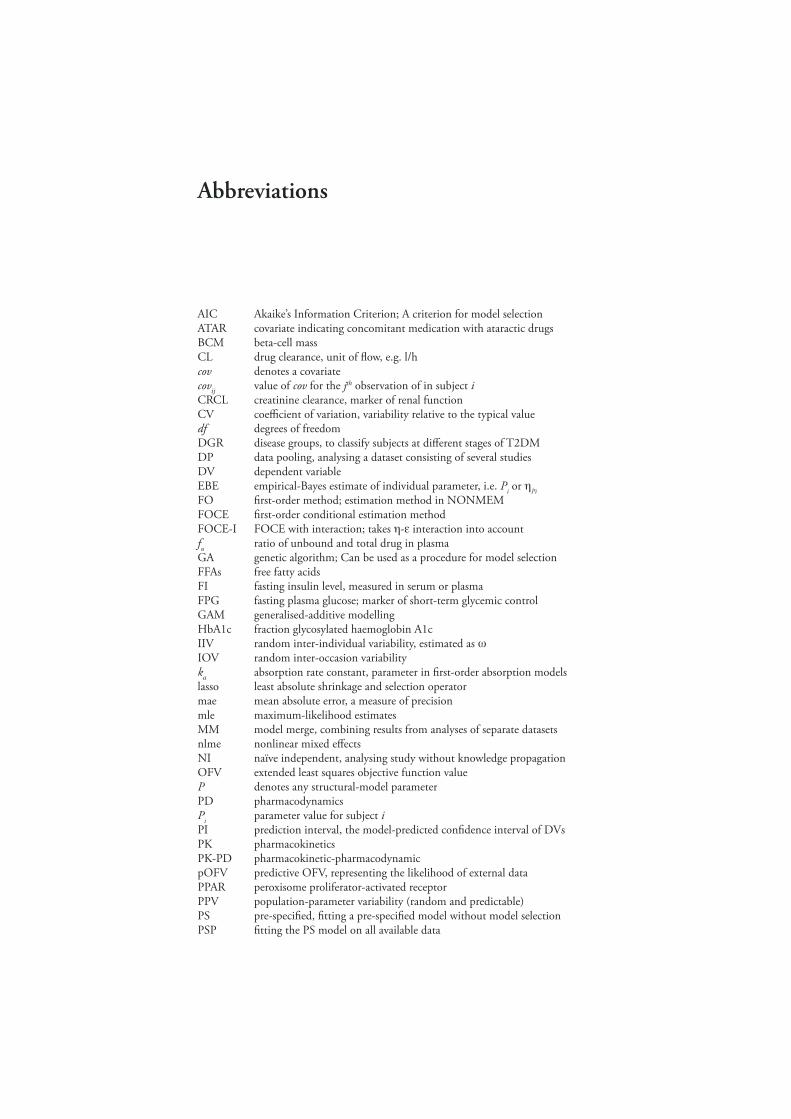
AIC Akaike’s Information Criterion; A criterion for model selectionATAR covariate indicating concomitant medication with ataractic drugsBCM beta-cell massCL drug clearance, unit of fl ow, e.g. l/hcov denotes a covariatecov

ij value of cov for the jth observation of in subject i

CRCL creatinine clearance, marker of renal functionCV coeffi cient of variation, variability relative to the typical valuedf degrees of freedomDGR disease groups, to classify subjects at diff erent stages of T2DMDP data pooling, analysing a dataset consisting of several studiesDV dependent variableEBE empirical-Bayes estimate of individual parameter, i.e. Pi or PiFO fi rst-order method; estimation method in NONMEMFOCE fi rst-order conditional estimation methodFOCE-I FOCE with interaction; takes - interaction into accountfu ratio of unbound and total drug in plasmaGA genetic algorithm; Can be used as a procedure for model selectionFFAs free fatty acidsFI fasting insulin level, measured in serum or plasmaFPG fasting plasma glucose; marker of short-term glycemic controlGAM generalised-additive modellingHbA1c fraction glycosylated haemoglobin A1cIIV random inter-individual variability, estimated as IOV random inter-occasion variabilityka absorption rate constant, parameter in fi rst-order absorption models

lasso least absolute shrinkage and selection operatormae mean absolute error, a measure of precisionmle maximum-likelihood estimatesMM model merge, combining results from analyses of separate datasetsnlme nonlinear mixed eff ectsNI naïve independent, analysing study without knowledge propagationOFV extended least squares objective function valueP denotes any structural-model parameterPD pharmacodynamicsPi parameter value for subject iPI prediction interval, the model-predicted confi dence interval of DVsPK pharmacokineticsPK-PD pharmacokinetic-pharmacodynamicpOFV predictive OFV, representing the likelihood of external dataPPAR peroxisome proliferator-activated receptorPPV population-parameter variability (random and predictable)PS pre-specifi ed, fi tting a pre-specifi ed model without model selectionPSP fi tting the PS model on all available data

PsN Perl-speaks-NONMEMr Pearson correlation coeffi cientrmse root mean squared error, a measure of precisionS insulin sensitivity, model parameter describing insulin resistanceSBC Schwartz’s Bayesian criterion; A criterion for model selectionSCM stepwise covariate modelling; A procedure for covariate selectionSEX sex, often confounded with gender. Gender is the socio-economic aspects that

follows with the (biological) sexSTS standard two-stage approachT2DM type 2 diabetes mellitusWAM Wald Approximation Method; A procedure for covariate selectionTVP

i typical value of parameter P, given covariate values for subject i

V volume of drug distribution (apparent)VPC visual predictive check, used for evaluation of nlme modelsWT body weightyij dependent variable, jth observation of in subject i

yij model prediction of dependent variable, jth observation of in subject i

ij residual error, weighted for the jth observation of in subject iPi the deviation from TVP

i in subject i

P magnitude of the IIV in parameter P, random-eff ects parameter magnitude of the intra-individual error

denotes a fi xed-eff ect that is estimated in the modelPcov the covariate coeffi cient for covariate cov on parameter PPpop the population typical value of parameter P

11

Covariate Model Building in NONMEM

1. Introduction

1.1. BackgroundWhen a drug is administered to a patient, a chain of events takes place, eventually leading to a treatment response. Normally, the drug molecules must fi rst be absorbed into the body and pass the liver before being distributed into the body tissues. Th e drug molecules reaching their site of action exert an eff ect by binding to specifi c target receptors. Th e treatment response for some drugs can appear almost immediately upon interaction of drug and receptor, but can also often be delayed (minutes to years). Th e delay may be due to a cascade of intermediate events and/or accumulation of the eff ect following the drug-receptor interaction.

Th us, at times it can be more practical to measure a marker of a drug-treatment eff ect rather than the so-called clinical endpoint, the hoped-for therapeutic outcome. For example, the treatment of high blood pressure is often evaluated by the reduc-tion of blood pressure although the clinical endpoint is the absence of heart attack or stroke, or even survival.Eventually, the eff ect of a single drug dose wears off , normally because the drug disap-pears from the body via metabolism and/or excretion into the urine. All events follow-ing drug administration can be divided into one of two processes.

1. Pharmacokinetics (PK) describes the fate of the drug molecules in the body after administration of a dosage regimen, i.e. what the body does to the drug.

2. Pharmacodynamics (PD), on the other hand, describes the action of the drug molecules in the body, i.e. what the drug does to the body.

Th e PK and PD of a drug are often described in the form of a model summarizing the important concepts in both qualitative and quantitative terms. Th e model is often longitudinal, meaning that it describes repeated measurements over time. Nonlinear models are used because the dependent variables (e.g. drug concentrations or drug eff ects) vary nonlinearly with time. Th e pharmacokinetic-pharmacodynamic (PK-PD) model can also be coupled with a disease model that describes the disease and its development over time. Th is is illustrated in Figure 1.

12

Jakob Ribbing

Figure 1. Illustration of a PK-PD model. Th e PK model describes systemic drug exposure. Th e PD model describes the response to the drug, measured in terms of changes to a clinical endpoint or a biomarker relevant for that endpoint. Th e endpoint, in turn, refl ects desired or adverse eff ects. Whereas the dosage regimen is the input to the PK model, the resulting exposure may be used as the input to the PD model. Th e collective model is called a PK-PD model.

Th e parameter in the model may have an associated physiological or mechanistic meaning, e.g. the volume of blood or plasma that is completely cleared of the drug per unit of time, or the maximum eff ect that the drug could produce if it were to occupy all its receptors. Highly mechanistic models can include processes of cell ageing or dif-ferentiation, or drug distribution into various organs based on blood fl ow and organ size, or known chemical or molecular interactions. Th e opposite of a mechanistic model is an empirical model, which describes the observations of response/exposure but has no scientifi c basis for its structure.

A population model, also called a nonlinear mixed-eff ects (nlme) model quantifi es the variability between individuals in the model parameters. It is vitally important to take inter-individual variability (IIV) into account in the model, rather than treating it as an independent error, both in order to describe the variability itself and to obtain an accurate description of the typical individual.1 Th e exposure and response to a drug varies substantially among patients. As a consequence, evidence that a treatment is safe and eff ective in the typical patient does not warrant its use in the whole patient population. Decisions in drug development are increasingly being made on model-based population analyses of the available information.2-7 Th is approach is encouraged by many of the regulatory agencies, e.g. the Food and Drug Administration in the USA and the Medical Products Agency in Sweden.2, 8, 9

It is often useful to explain the variability in a parameter using a covariate model that describes the relations between covariates and parameters.5, 6, 10-12 Whereas a parameter is a fi xed quantity estimated according to the model, a covariate is an independent variable that contains information on a parameter, i.e. the parameter depends on the covariate. For example, small patients have smaller volume into which the drug is distributed (V) and lower clearance of the drug from the body (CL). Th is is because CL and V are parameters that depends on the body size.13 Th is is the main reason to that children often receive lower doses that adults. Another example of a covari-ate-parameter relation is a positive correlation between markers of renal (i.e. kidney) function and the renal drug clearance. A common marker of the renal function is the so-called creatinine clearance (CRCL) which can easily be calculated from the level of serum creatinine and patient demographic characteristics. A covariate model can be

DoseRegimen

ExposureFor example concentration-time profile

ResponseClinical or surrogateendpoint or biomarker

PK Model PD Model

Disease Model

PK-PD Model

13


used for identifi cation of patient subpopulations at risk for sub-therapeutic or toxic eff ects and to subsequently individualise the treatment and the initial dosage regimen. Furthermore, such a model is useful for identifying the need for and aiding the design of new studies in the drug development process. If the identifi ed covariate relations are in line with the literature or prior expectations, the covariate model supports the structure of the other parts of the model. Th us, the development of a covariate model may also be viewed as a component of the model evaluation.

1.2. Nonlinear Mixed Eff ects ModelsA PK-PD model contains so-called mixed eff ects if it has two or more levels of random eff ects, i.e. where the random variability in the parameters is treated separately from the residual (intra-individual) variability. Th e term “mixed” is used because the model estimates both fi xed and random eff ects simultaneously. Typically, the random eff ects form a hierarchy in the sense that the random components in the parameters are constant within an individual whereas the residual variability may change for each observation.

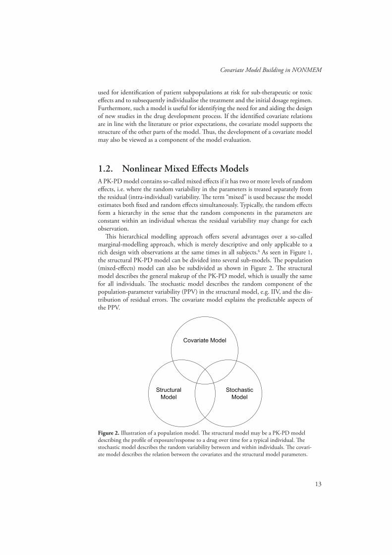
Th is hierarchical modelling approach off ers several advantages over a so-called marginal-modelling approach, which is merely descriptive and only applicable to a rich design with observations at the same times in all subjects.6 As seen in Figure 1, the structural PK-PD model can be divided into several sub-models. Th e population (mixed-eff ects) model can also be subdivided as shown in Figure 2. Th e structural model describes the general makeup of the PK-PD model, which is usually the same for all individuals. Th e stochastic model describes the random component of the population-parameter variability (PPV) in the structural model, e.g. IIV, and the dis-tribution of residual errors. Th e covariate model explains the predictable aspects of the PPV.

StructuralModel

Covariate Model

StochasticModel

Figure 2. Illustration of a population model. Th e structural model may be a PK-PD model describing the profi le of exposure/response to a drug over time for a typical individual. Th e stochastic model describes the random variability between and within individuals. Th e covari-ate model describes the relation between the covariates and the structural model parameters.

14

Jakob Ribbing

A wide variety of structural models are relevant to the area of PK-PD modelling. A few of these are described in the Methods section but no attempt is made to provide an overview of diff erent structural models in this thesis. For this introduction, it is suffi cient to describe the prediction of the dependent variable (exposure or outcome) in an individual according to

(1)

where xij are design variables (e.g. regimen and time) and Pij is the individual param-

eter vector for the jth observation in individual i. Pij is a function of population param-

eters, random-eff ects parameters and covariates as described below. Th e subscript j can be dropped if individual parameters are constant over time. Th is is normally how parameters are viewed: as constants that are estimated in the model. Th e independent variables that may be input to the model include, for example, dose, time and covari-ates. Th e dependent variables are predicted by the model. Th ese may be drug exposure, response or outcomes that may not be measured directly, such as the sensitivity to insulin of a diabetic patient. Th e remainder of this subsection explains the concept of the stochastic model and the next subsection explains the covariate model. For brevity, the explanation is essentially limited to concepts relevant to the work in this thesis.

Th e random components are most often assumed to be derived from a parametric distribution. An individual parameter (Pi) is commonly distributed according to

(2)

where, regarding the parameter P for subject i, TVPi is the typical parameter value and Pi is the random eff ect that is normally distributed around zero, with standard devia-

tion P refl ecting the IIV. Th is parameterisation assumes that the random variability around the typical value has a log-normal distribution, which is often reasonable for parameters that have a lower (physiological) boundary at zero. If the parameter also has a higher boundary at one, a logit transformation can be used to reshape the distri-bution. Th is will eff ectively restrict all individual parameter values between zero and one and is parameterised according to

(3)

Further, if some individuals have been observed several times on multiple occasions and there is a random variability in Pi over time, Equation (2) can be expanded to include inter-occasion variability14 (IOV) according to

(4)

where, regarding parameter P on occasion k in subject i, κPk is the random eff ect nor-mally distributed around zero with standard deviation P refl ecting the IOV. Th e IOV can only be separated from the residual error if some individuals have been observed several times on the same occasion.

Th e model predictions (yij) of the observed values (yij) are associated with a residual

error which can be additive, proportional/exponential, or a combination of the two.

Pii iP TVP e

ˆ ,ij ij ijy f x Puur

ln 1

ln 11

i i Pi

i i Pi

TVP TVP

i TVP TVP

eP

e

Pik Piik iP TVP e

→

15


Due to approximations in the estimation procedures and for numerical stability, the error may be assessed on log-transformed values. Th e three error models used in this thesis are described by

(5)

(6)

(7)

where, for the jth observation in subject i, ij is the individually weighted residual error that has a normal distribution centred around zero and a standard deviation .

represents the IIV in the residual-error magnitude15 and if is not zero repre-sents the typical residual-error magnitude within an individual. Th e residual error can represent assay/measurement error and errors in the recorded time and dose as well as model misspecifi cation, e.g. non-adherence to therapy16-18 that is not accounted for. Usually, even for well controlled clinical trials, assay error does not constitute the major part of .15

Correlations between individual parameters or between residual errors can be included in the model. Individual parameter correlations not associated with covari-ates in the model are included as covariance between diff erent random eff ects ( s). Correlations between the intra-individual errors ( ) may either be included as a func-tion of time within the same dependent variable and individual (auto-correlation) or as a covariance of between diff erent dependent variables measured at the same time, e.g. observations of drug and metabolite or repeated assays of the same sample.15 Unless otherwise noted, the random eff ects are assumed to be independently and identically distributed, i.e. without any correlation and not according to Equation (7) above.

1.3. Th e Covariate ModelA covariate model describes the relations between covariates and parameters. Th is introduction merely discusses the relation to structural model parameters. However, covariates may also infl uence the random eff ects distribution, e.g. the magnitude of the IIV or residual error15 or the probability of belonging to a certain mixture.19, 20 A mixture could for example consist of poor and extensive drug metabolizers.

1.3.1. What is a covariate?Covariates are characteristics describing the patient, the conditions of the drug treat-ment or other factors potentially infl uencing the outcome. Th e covariates may be constant within an individual (e.g. sex) or changing over time (e.g. age). Potential covariates in a PK-PD model include:

ˆ 1ij ij ijy y

ˆln lnij ij ijy y

ˆln ln iij ij ijy y e

16

Jakob Ribbing

• Demographics: age, weight, sex.• Markers of organ function: CRCL, alanine aminotransferase, bilirubin.• Environmental indicators: concomitant medication, smoking, season, gender.21

• Others: disease state or progression, quantifi ed on an assessment scale or by a biomarker; genotype of a metabolising enzyme or a binding site; other phenotype, e.g. the ratio of unbound and total drug in plasma (fu); or other laboratory mea-surement.

In nlme models, dose and time are normally not considered as covariates but rather as variables that are an integrated part of the structural model. Th is may also be the case for a biomarker which is on the mechanistic pathway to the actual treatment response. Th e biomarker may be included as part of the structural model and this variable would then be observed with a residual error as a dependent variable. Th e covariates, on the other hand, are included in the model as if measured without any error, as independent variables.

1.3.2. What is a true covariate?We can view all PPV as being predictable by a (large) set of latent variables.22 How-ever, these latent variables may be unknown and immeasurable. On the other hand, the covariates that we actually do measure can be partially correlated with these and may either be causative to (e.g. sex) or aff ected by (e.g. creatinine clearance) latent variables. In this thesis, the pragmatic view is taken that a true covariate is one that, among the investigated covariates, carries unique information on a structural model parameter.

If data are generated by simulation from a model, the true covariates are those used in the simulation model, whereas all others are defi ned as false. However, in the event that one of the true covariates is not available for investigation, any other covariate that carries unique information on the unavailable covariate can instead be defi ned as true. Regarding real data, the distinction of true/false becomes pointless, since it is impossible to reject any covariate as false. Instead, one can discuss whether a covari-ate relation is important or clinically relevant, or if it in any other way supports the model.

1.3.3. Multiplicative and additive parameterisationTh e contributions of diff erent covariate eff ects on a structural model parameter are often combined as a multiplicative covariate model according to

(8)

where CovEff ectPcov,ij is the fractional change in the parameter due to the covariate (cov) in individual i at time point j. Ppop is the population typical value of parameter P (i.e. TVPij) for a subject i with all Ncov covariates equal to the median at time j. Th e subscript j can be dropped if the level of the covariate is constant over time, as for e.g. sex and race. An additive covariate model is described according to

cov

cov,cov 1

(1 )N

ij Ppop P ijTVP CovEffect

17


(9)

Multiplicative parameterisation contains a fi xed-interaction component. Th is fi xed interaction can sometimes be useful for mechanistic reasons. One example of this is the two covariates body size and genotype of a metabolizing enzyme, and their rela-tion to drug clearance (CL). A poorly metabolizing genotype that reduces a parameter by 50% combined with a small body size that reduces the parameter by the same degree will not together result in a 100% reduction of CL, but rather in a 75% reduc-tion. However, the main rationale for using multiplicative parameterisation is that it is practical to set boundaries on Pcov so that TVPij is confi ned to positive values (zero often being a physiological boundary for the structural model parameters). Th is can also be applied to additive parameterisation. However, in the additive case it is only possible to avoid negative values of the structural model parameters for the combina-tions of covariate values that are in the dataset - not for the patient population as a whole. In this thesis, multiplicative parameterisation is used without exception. For brevity, a covariate model will sometimes be referred to as linear or piece-wise linear without mentioning the fact that it is multiplicative.

1.3.4. Categorical covariatesA categorical covariate can only attain two or more discrete values, or levels. If these can be ordered, the covariate is said to be measured on the ordinal scale. Examples of such covariates are tumour stages and categorization of a continuous variable. If the variable cannot be ordered, it is said to be measured on the nominal scale. An example of such a covariate is race. However, the distinction between ordered and non-ordered covariates is only important if the covariate has more than two levels. Th e eff ect of a non-ordered categorical covariate on a parameter P can be expressed relative to the reference level according to

cov

cov,cov 1

1N

ij Ppop P ijTVP CovEffect

cov1

cov, cov2

cov3

0 at reference level

at level 1

at level 2

at level 3

ij

P ij

P ij P ij

P ij

if cov

if cov

CovEffect if cov

if cov(10)

the coeffi cient PcovL is the fi xed eff ect that establishes the impact of belonging to level L relative to the reference level. As an example, with the reference level at 0, an ordered categorical covariate can instead be parameterised according to

cov1

cov, cov1 cov2

cov1 cov2 cov3

0 at 0

at 1

1 at 2

1 1

P

P ij P P

P P P

if cov

if cov

CovEffect if cov

i at 3f cov

(11)

18

Jakob Ribbing

where PcovL is now a coeffi cient describing the eff ect relative to the previous level, i.e. L-1. Restricting Pcov2, Pcov3 , etc. to positive values confi nes the eff ect to be either increasing or decreasing as the level of the covariate increases. If this is not a reason-able assumption Equation (10) can be used, although the covariate is measured on the ordinal scale.

1.3.5. Continuous covariatesTh e eff ect of a continuous covariate (i.e. interval or ratio scale) on a parameter (P) is often expressed relative to its median in a relevant patient population, denoted cov. Th e most common functional forms of covariate relations are linear, piece-wise linear, power and exponential. Th e linear relation is parameterised according to

(12)

where Pcov is the covariate coeffi cient, i.e. a fi xed-eff ects parameter. Th e piece-wise linear relation with a break point at the median covariate value is parameterised according to

cov, cov cov covP ij P ijCovEffect

cov1

cov,

cov2

cov cov cov cov

cov cov cov cov

P ij ij

P ij

P ij ij

ifCovEffect

if (13)

Th e break point(s) can be estimated instead of pre-specifi ed as the median.23 However, such an estimation may be unstable and consumes extra degree(s) of freedom (df). Th e functional forms for the power and exponential covariate models are

(14)

(15)

Examples of possible shapes describing the above functional forms are shown in Figure 3.

cov

cov,

cov1

cov

P

ijP ijCovEffect

cov1 cov cov

cov, cov2P ij

P ij PCovEffect e

19


Figure 3. Examples of shapes that can be formed by four common functional forms of a covariate relation. Th e piece-wise linear and exponential relations are more fl exible and con-sume an extra degree of freedom (df ) whereas the power and linear relations rely more on assumptions. Th e choice of which parameterisation to use depends e.g. on the amount and range of the data, the signal in the data and mechanistic preferences in combination with the purpose of the model.

1.3.6. Covariate transformationMany nonlinear covariate relations can also be investigated in the framework of linear models by the introduction of dummy covariates. Th ese include piece-wise linear models with pre-defi ned breakpoints, log-linear models, and ordered or non-ordered categorical covariates. For example, a non-ordered categorical covariate with three levels can be replaced by two dummy covariates, the fi rst dummy being one if the original covariate is level 1 and zero otherwise, the second dummy being one if the original covariate is level 2 and zero otherwise. Instead of the categorical covariate, the two dummy covariates can be included as two linear models according to Equation (12).

1.4. Software for Model FittingFitting the model means estimating the model parameter values resulting in the best fi t to the available information (e.g. data). Th e traditional approach to estimating the parameter values for a population model is to perform the analysis in two stages, the

Covariate value

Typ

ical

val

ue o

f a s

truc

tura

lm

odel

par

amet

er

0

20

40

60

80

0 20 40 60 80 100

exponential relations (df=2) linear relations (df=1)

piece wise linear relations (df=2)

0 20 40 60 80 100

0

20

40

60

80

power relations (df=1)

20

Jakob Ribbing

standard two-stage (STS) approach. First, the individual parameters are estimated separately for each individual. Th en, the parameter variability is calculated based on the individual estimates obtained in the fi rst stage. Th is approach requires a sub-stantial number of observations in each individual, usually three to fi ve observations per subject for each structural model parameter. However, this number is highly dependent on how informative the data are.24 For practical reasons and because of the often invasive nature of the observations (blood samples), the data possible to obtain from patients are often sparse, i.e. a few samples per individual. Th erefore, the STS approach results in infl ated (upwardly biased) estimates of IIV and is also limited to models with few parameters. In addition, the STS may provide biased estimates of the typical profi le, since individuals with too few observations have to be omitted; for example, subjects with fast elimination will have few measurements above the limit of quantifi cation. Th ese problems taken together was the motivation for development of the NONMEM software that was introduced in 1980 as the fi rst software performing hierarchical nlme modelling.1, 25-28 For nlme models describing clinical data, it is still the most widely used regression software both in academia and industry.9, 25, 29

All fi tting of nlme models in this thesis has been performed using NONMEM30 software. Th is software estimates the parameters of a parametric nlme model, accord-ing to an approximate maximum likelihood. Th e same is true for the SAS-procedures NLMIXED (NLINMIX/NLMEM) using (non-adaptive) Gaussian quadrature,31, 32 WinNonMix33 and NLME34 in S-Plus. Exact maximum-likelihood estimation is per-formed by NLMIXED using the adaptive-Gaussian quadrature35 in SAS, SAEM36, MCPEM37 and PEM38. All of the above software packages use a Bayesian (i.e. hier-archical) approach in the sense that the population parameters inform the individual parameters; cf., for example, Equation (2). NONMEM can also make use of a so-called frequentist prior to propagate the prior knowledge of the parameters into the current analysis.39 Full Bayesian methods make use of the prior parameter distribution without parametric assumptions. Software packages for this approach include Win-BUGS40 and MCSim41. Software packages for nonparametric maximum-likelihood estimation include NPEM42, 43 and NPML44.

Despite the fact that the developers have already run out of unique abbreviations and acronyms for the words Nonlinear Mixed-Eff ects Models, there is still continuous development of new software for nlme models. Further, many of the old software packages are being upgraded with new functionalies and new estimation methods. In the next subsection we focus on the NONMEM estimation methods that have been used in this thesis.

1.5. Estimation Methods in NONMEMParameter estimation in NONMEM is based on maximizing the likelihood of the data, given the model. An iterative search within the parameter space terminates at a maximum likelihood and the parameter estimates obtained in this manner are called the maximum-likelihood estimates (mle). An approximation of the likelihood is obtained via the extended least squares objective function value (OFV). Assuming that the random eff ects are normally distributed, the OFV is “up to a constant” equal to minus twice the natural logarithm of the likelihood.30, 45

21


Th e random eff ects on the nonlinear structural model parameters often preclude the obtainment of an analytical solution to the objective function.29, 35 In NONMEM, this is approached by approximating the OFV by a linearization of the nonlinear model. Th e fi rst-order method (FO) uses a fi rst-order Taylor-series expansion at =0 whereas the fi rst-order conditional estimation method (FOCE) performs the same linearization with respect to . Interactions between and can be accounted for by using the FOCE with interaction (FOCE-I). In this thesis FOCE-I was used for application of the error models in Equations (5) and (7). In the former, the interac-tion is implicit since is multiplied by the model prediction which in turn is a func-tion of the s, cf. Equations (1) and (2).

1.5.1. Individual empirical bayes estimates and shrinkageNONMEM provides the individual parameter estimates, e.g. Pi or Pi, as empirical-Bayes estimates (EBE) generated during the estimation procedure (e.g. FOCE and FOCE-I) or posthoc (FO). Th ese individual parameter estimates may tend to shrink towards the population typical value ( Pi=0) in comparison with the true individual parameter values. Th is reduction in the variability of an EBE is called -shrinkage. An extreme example of shrinkage is PK and drug-specifi c PD parameters in patients who receive placebo instead of active treatment. Since, for these parameters and in this context, the data from the placebo recipients contain no information, the individual estimates rely solely on the typical parameter value, TVPi. Th is means that all avail-able information comes from the total population, resulting in complete shrinkage in this group. However, the shrinkage induced by sparseness of data (information about a parameter) is more harmful than a complete lack of information. Th is will be discussed further in subsection 1.8.1.

Th e degree of -shrinkage can be assessed as the standard deviation of the Pi rela-tive to the IIV estimated for the same parameter in the same dataset.46 Alternatively, if Pi is biased, i.e. not centred around zero, the root mean square can be evaluated instead of the standard deviation, according to

2

11P

N

Pii

P

shrinkageN (16)

where N is the number of subjects in the dataset. Bias in the s is of interest for diag-nostic purposes.46 Equation (16) does not indicate any shrinkage due to bias, since in this thesis, the degree of shrinkage and bias in the s are treated separately.

1.6. Model Development and SelectionIn drug development, model-based population analysis is often used in an explor-atory manner for “learning”, but model-based confi rmatory analysis is also increas-ingly applied.3, 5, 6, 9 Whereas a confi rmatory analysis is focused on testing a pre-speci-fi ed hypothesis, an exploratory population analysis can take new concepts and ideas into account during the process. Th is is achieved by investigating a large number of hypotheses based on, for example, informative graphics as well as statistical testing.47

22

Jakob Ribbing

Often, the model is developed in several stages. In the fi rst stage, the structural and stochastic models are developed, starting with a simple model and expanding the complexity when supported by the data. Highly infl uential or pre-specifi ed48 covari-ate relations can be included in the model even at this early stage. Estimation of IIV for all structural model parameters and correlations between all random components is seldom possible in NONMEM because of lack of information in the data. Th us, there is often considerable work involved at this stage to develop the appropriate structural, IIV, and residual-error models. Th e fi rst-stage model is called the base (or basic) model in this thesis.

In the second stage, the explanatory value of the covariates is investigated on the parameters of the base model. Covariate relations that explain part of the IIV in a parameter can be included in the model at this stage. In the third and last stage, the stochastic model is re-evaluated and refi ned. Preferably, other parts of the model are constantly re-evaluated throughout the developmental process. Even so, there is a problem with this stepwise approach to model selection in that the selection of one model feature may be conditional on another model feature.49 Th is interaction between diff erent parts of the model can be handled by investigating all combinations of all model features. An attempt to achieve this using a genetic algorithm (GA) has been made.50 However, since the number of combinations is often vast; this approach is currently only possible in rather limited modelling exercises. Furthermore, the cri-teria for selection that can be used in an automated procedure are also limited at pres-ent. Th e most common approach is to increase (or decrease) the model complexity in a stepwise manner. Th is is explained further in the next subsection.

Th e current standard analysis results in a single nlme model (the fi nal model) rather than a set of possible models.51-53 Th is fi nal model summarizes and quantifi es the knowledge gained from the analysed data, possibly also including information (data) or knowledge (parameter distributions or values) from analyses of other stud-ies.6, 39, 54 Inferences are drawn from the fi nal model as if no model selection had been performed based on the information (data) that was used to estimate the model parameters.55

Depending on the purpose of the model, the criteria for selecting one model over another can include• mechanistic plausibility and prior beliefs: consideration of model structure and

parameter estimates, the former also setting a limit to what is investigated in the fi rst place56

• plots displaying goodness-of-fi t and other graphics57, 58

• successful convergence or obtainable covariance matrix of the estimates• statistical signifi cance: p-value, Akaike’s information criterion (AIC), Schwartz’s

Bayesian criterion (SBC ), etc.10, 50, 59, 60

• relevance: clinically unimportant features may be ignored in favour of model par-simony61

• simulation properties62-64

• predictive performance: in internal or external validation65-68

• parameter precision: e.g. avoiding colinearity due to the data/model69 70

• infl uential individuals:69, 71 is the model feature promoted by only one or a few individuals?

• other model fi t as diagnostics72

• other practical matters: e.g. computer run-time

23


1.6.1. Stepwise selectionStepwise-selection procedures currently dominate model selection in nlme modelling. Th is approach can be exemplifi ed by a system of selection based solely on p-values. It should, however, be noted that the criteria can include other more subjective condi-tions or terms, as mentioned above. If FOCE (or FOCE-I) is used, the diff erence in OFV between two hierarchical models is approximately chi-square distributed with the appropriate df.73, 74

In forward selection, the model complexity (model size) is increased from a simple model. Th e features of interest that can be fi tted are evaluated by including them one at a time into the nlme model. Th e feature that performs best according to the p-value is included into the model if it is statistically signifi cant. Subsequently, all other model features are re-evaluated in the new model and a second feature is included if it is signifi cant. Th e procedure stops at the full-forward model when no further model features are statistically signifi cant. An alternative approach is backward elimination. Th e starting point is a model that initially includes all features of interest, called the full model. Elimination is performed until only statistically signifi cant features remain. When this approach is possible, the end result is often as good as an all-subset selec-tion, which investigates all combinations of the diff erent model features of interest. Th is is not always the case with forward selection.75 However, the presence of features that are mutually exclusive or inestimable in combination due to correlations between the estimates often prevents the use of backward elimination techniques. Further, many ideas that are generated during an exploratory analysis cannot be included in the initial model. Because of this, backward elimination can only be used for part of the model-building procedure. Another alternative is to use forward selection with a less strict (i.e. a higher) p-value. Th e full forward model obtained in this manner is then refi ned by backward elimination using the same or a stricter p-value. Th is proce-dure is called “forward inclusion and backward elimination” and is commonly applied in the selection of a covariate model.10

1.7. Th e Base ModelTh e base model is the starting model in a covariate investigation. Th e model can contain covariates, however only for pre-specifi ed covariate relations included in the model without testing. Th e pre-defi ned covariate model can be fi xed so that no covari-ate parameters are estimated or the structure of the covariate model can be fi xed while the parameters are estimated from data. An example of the former is assuming an allometric relation between PK parameters and a measure of body size.76 Estimating the covariate model parameters is necessary when information about the covariate relationship is qualitative but insuffi ciently quantitative. An example of such a situa-tion is the use of CRCL77 as a covariate to explain variability in the clearance of a drug which is known to be mainly eliminated via glomerular fi ltration.12

24

Jakob Ribbing

1.8. Selection of the Covariate ModelIn an exploratory analysis, there are often a large number of covariates available which would be interesting to test on one or more structural model parameters. Th ere are several reasons for selecting a subset of these instead of including all of them in the fi nal model. Th e fi rst is that a model containing all the potential covariate-parameter relations may not be estimable, i.e. the estimation would not converge in NONMEM. Second, most of these potential covariate eff ects are unimportant. Consequently, to obtain an overview of which covariates are important, the less important or uncer-tain covariate relations should be removed. Also, estimation of uncertain relations is imprecise and removing these improves the performance of the model for predicting external data, i.e. improves the predictive performance. Naturally, predicting the out-come in new patients or future events is often an important objective of the model.

Another reason for reducing model complexity is that potential covariates are often correlated. If all of them are included a high correlation between the estimates of the covariate coeffi cients arises. Th ese coeffi cients are then estimated with high impre-cision,70 making it impossible to decide which of them are important or clinically relevant. Extrapolation of such a model outside the current range of the data can therefore be unfortunate. One solution to this problem is to reduce the number of investigated covariates by removing redundant (correlated) covariates based on the relevant current literature78 and to retain the rest in the model, i.e. a pre-specifi ed model. Th is is a good approach for obtaining correct confi dence intervals and for summarizing current knowledge of clinical relevance. However, this approach does not explore diff erent functional relations or which of the correlated covariates are important.

For the reasons mentioned above, a subset of the potential covariate relations is often selected for the fi nal model. Th e actual selection of which relations to include can be made after investigating the results of including each of them in the nlme model. Th ese procedures are collectively called selection within NONMEM. Alterna-tively, the outcomes of the diff erent relations can be investigated outside NONMEM, after which one or several selected models are investigated within NONMEM. Th e latter alternative, which is called selection outside NONMEM, has not been investi-gated in this thesis work but is extensively discussed in next subsection.

1.8.1. Covariate selection outside NONMEMTh e main advantage of selecting the covariate model outside NONMEM is that an investigation within NONMEM is computer intensive, resulting in long computer run-times and/or high demands on a computer grid. Th erefore, a seemingly appeal-ing approach is to perform graphical inspections of the relations between covariates and the EBE of individual parameters to fi nd the relevant relations. However, if data are sparse, this may lead to shrinkage of the EBE towards the typical parameter value so that a clinically relevant relation may become distorted in its shape or appear as unimportant or falsely important.9, 46

A statistical evaluation of a relation can be used to pick up even weak trends that may be invisible in a graphical inspection. Th is is commonly used for identifying the covariate model using generalized-additive modelling (GAM).11 Th is approach is not

25


CRCL (ml/min)

CL

(l/h)

2

4

6

8

50 100

Model including covariate relation

50 100

Model without covariate relation

appropriate for handling time-varying covariates or randomly time-varying param-eters, i.e. those with IOV. Investigating covariates on parameters that do not have any IIV according to the base model is not possible at all. Further, the issue of shrinkage creates additional problems unless the data contain rich information on the inves-tigated individual parameters. A modest correlation between the structural model parameters can result in a false correlation between the individual parameters. Th us, a relation between a covariate and one parameter may induce a false relation between the covariate and several other parameters. Further, shrinkage is more pronounced for the individual parameter values that are implausible according to the nlme base model. Th is changes the apparent shape of the relation between covariate and parame-ter. Th is is illustrated in Figure 4.Due to shrinkage, covariate relations may be hidden, induced or distorted when using GAM.46

Figure 4. Illustration of the eff ects of shrinkage. Th e left panel displays the individual esti-mates of CL from the model including an important relation between CL and CRCL. Th e right panel displays the same estimates from a model not including the covariate relation. Each circle represents a separate individual. Th e solid line is a smooth of the data whereas the broken line represents the expected CL according to the model used for simulation. Including the covariate relation, the two lines agree well. However, if not including the important rela-tion, the shrinkage increases from 0.37 to 0.77 and the quality of the individual estimates is reduced. As a result, the relation between CL and CRCL is distorted and appears to be non-linear. Th e data was simulated so that information on CL is independent of the value of the parameter, meaning that this is a pure eff ect of shrinkage.

When GAM or graphical analysis is used for covariate selection, it is advisable to evaluate the covariate relation in the parameter space and not the relation with Pi. A linear relation in GAM will otherwise translate to an exponential relation in the nlme model, given that IIV is distributed according to Equation (2). If any covari-

26

Jakob Ribbing

ate is already included in the nlme model, this should be accounted for by regress-ing Pi /TVPi on covi. Alternatively, for additive-covariate parameterisation, Pi-TVPi should be used, cf. subsection 1.3.3. If shrinkage is a problem for any of the investi-gated individual parameters, two further actions can be taken to slightly reduce these eff ects. Th e fi rst is to evaluate other functional relations (shapes) in addition to the one selected by GAM. More importantly, only the most signifi cant relation in GAM should be included in the nlme model. Th en, after fi tting the new nlme model in NONMEM, a new GAM analysis can be made based on the new individual param-eters. Th ese two steps are performed until no relation is found by GAM or until inclu-sion in NONMEM is no longer supported. Alternatively, all relations identifi ed by GAM can be included in the nlme model initially and then subsequently re-evaluated using backward elimination within NONMEM.

A completely diff erent approach performing the covariate selection outside NONMEM is to use Wald’s approximation to the likelihood ratio test (WAM).59 Th is method requires the point estimates and the covariance matrix of the estimates from a full model fi t including all covariate relations of interest. If these can be obtained, WAM may be used to quickly perform an all-subset selection, investigating all pos-sible combinations of covariates and parameters. Th e most promising models are identifi ed outside NONMEM by this approach and subsequently evaluated within NONMEM. Th e main criticism of this approach is that it is often impossible to obtain the variance-covariance matrix of the parameter estimates for the full model from NONMEM. It may also be diffi cult to obtain these by non-parametric boot-strapping due to long run times, parameters ending up at the boundaries, or other failed convergences in NONMEM. Th ese problems are partly due to a tendency of pharmacometricians to investigate more relations than supported by the data.79, 80 Th ese problems seem to be the main reason for the less wide-spread use of WAM, compared to alternative methods. Another potential objection to WAM is that it only selects covariate-parameter combinations whereas the functional form, the originator suggests, should be determined using graphical inspection.59 As mentioned above, this is inappropriate for individual parameters with extensive shrinkage. Further, the graphical approach has additional complications when investigating the func-tional form in a multivariate setting. Th e WAM originator further concludes that the approximation may work less well for models with a high degree of nonlinearity. Unfortunately, these include many PD models and nonlinear PK models (i.e. nonlin-earity in the diff erential equations). Th e WAM is an appealing method for covariate selection where the degree of nonlinearity is low and either investigation of diff erent functional forms is unwished or possible to investigate without problems of shrinkage or covariate correlations.

1.8.2. Covariate selection within NONMEMCovariates are often selected within NONMEM in a stepwise manner, e.g. using the procedure stepwise covariate modelling (SCM).10 Th e stepwise procedures have been extensively investigated in traditional statistics and a few of the associated problems are outlined below.

SCM often uses a p-value as an indicator of when to halt inclusion or deletion of further covariate coeffi cients, i.e. as a stopping rule. In general, several covariates

27


are investigated, possibly on a number of structural model parameters and in several diff erent functional forms. Th erefore, the overall type-I error rate (i.e. the probability of including one or more false covariate coeffi cients into the model) is much higher than indicated by the required p-value. Th is is a problem of multiple comparisons.81 To correct for this, a stricter p-value is often used in the selection, although this can in turn result in omitting relations that are actually important. Further, correction of the p-value is only approximate or even arbitrary. Because of correlations, fi nding the value that corresponds to the overall type-I error rate is very computer intensive. Th us, although the p-value is used as a criterion for selection based on the ideas of hypothesis testing, the actual strength by which the null hypothesis has been rejected is unknown in the case of multiple comparisons. When predictive performance is the main objective, a stopping criterion focusing on this can be expected to perform better. Cross-validation is such a criterion.82

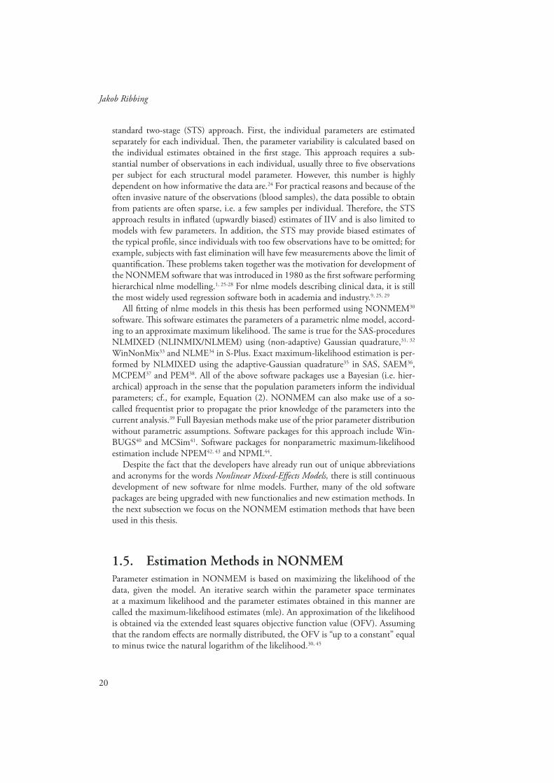
Th e coeffi cients selected by SCM are exaggerated because of selection bias. A relation that seems important is often statistically signifi cant whereas one which by random chance seems less important is left out. In this manner, the selected relations are on average more important than they would have been if the full model had been estimated without selection.

A systematic diff erence is called bias. In this context it is called selection bias since it is caused by two elements in the selection procedure; the requirement of statistical signifi cance and the competition between correlated covariates.83 An illustration of extreme selection bias is presented in Figure 5. Selection bias can decrease the predic-tive performance of a model. Th is is a problem for all selection procedures which do not include shrinkage of the selected covariate coeffi cients, so that the magnitudes of the coeffi cients are reduced compared to the mle. We use the term “shrinkage” for both penalized estimation of covariate coeffi cients and the -shrinkage in that arise due to sparse data (cf. subsection 1.5.1). Although the two kinds of shrinkage are sound for the same reasons they are treated as separate issues in this thesis.

Th e problem of selection bias due to SCM has been investigated for a typical PK analysis. Th e conclusion was that selection bias seems to be a minor problem.60 How-ever, the simulations in this investigation were based on a model that was obtained by applying SCM to a typical PK dataset. Th us, the coeffi cients in the model are expected to be biased to a larger magnitude, increasing the inclusion rates and decreasing the selection bias when the selection was subsequently investigated on the simulated data. Except for this case study, the problem of selection bias has not been investigated in nlme models. Th e degree to which the investigation of several covariates can further infl ate the selection bias due to competition is also unclear.

28

Jakob Ribbing

Figure 5. Illustration of the distribution of estimates from 7400 replicated studies simulated with a weak covariate coeffi cient. Th e grey bars represent all 7400 estimates whereas the black bars represent a subset of 611 estimates where the covariate was retained in the model due to statistical signifi cance. Th e selection bias is very clear in this example. All estimates are exag-gerated when selected from a dataset of such a small size (20 subjects). Th e distribution of all estimates (grey bars) is centred around the true value of the covariate coeffi cient.

Associated with selection bias, SCM is very categorical when selecting covariates. A relation is either included according to the mle or completely excluded from the model. Th is categorical selection leads to highly variable estimates and reduces the predictive performance of the model. A selection procedure such as the least absolute shrinkage and selection operator (lasso) method, which shrinks the coeffi cients for uncertain relations has been found to perform better in this context.84

Compared to all-subset selection, the stepwise approach may not come across the optimal combination of predictors in its search path. Th is can especially occur when forward selection is used on a set of predictors that perform well together but poorly alone.85 Th is problem can be overcome by starting a backward elimination of the full covariate model.75 However, with many covariates or diff erent functional relations to investigate, this approach becomes impossible or at least very time consuming.

SCM allows excessively many relations to be tested. Th e fi nal covariate model may not show any signs of overfi tting, even though too many hypotheses were tested before arriving at the fi nal model. Translating the general advice in traditional statis-tics79, 80 to covariate selection in mixed-eff ects modelling indicates that it often harms the predictive performance of a model if more than one covariate parameter per 10-20 individuals in the dataset is investigated on each structural model parameter. Fewer covariate parameters should be investigated for parameters on which information is sparse or when categorical covariates are investigated. However, this rule-of-thumb is highly dependent on the quality of the hypothesised relations and thus highly depen-dent on the drug, the investigated patient population, and the therapeutic area. Th e number of investigated covariate parameters includes, e.g. diff erent functional forms for a relation that has been considered in a graphical analysis prior to SCM. Because of this, the actual number of investigated covariate parameters is often unknown.

0

500

1000

1500

2000

-0.2 -0.1 0.0 0.1 0.2 0.3

Estimate of the covariate coefficient

Fre

quen

cy

29


1.9. Th e Lasso in Ordinary Multiple RegressionTh e lasso method is a penalized estimation technique for linear models.84 However, many non-linear covariate relations can also be investigated in the lasso framework, by the creation of dummy covariates as described in subsection 1.3.6. Before using the lasso, the covariates must be standardized to zero mean and standard deviation one. Th en, the lasso estimates of the regression coeffi cients are as in ordinary least-squares regression but subject to restriction on the magnitude of the coeffi cients according to

(17)

where ´k is the regression coeffi cient operating on the standardized covariate k, and the amount of shrinkage is determined by the value of t, the tuning parameter. In an nlme model, ´k corresponds to Pcov in Equation (12).

For low values of t, the implication of this restriction is that some covariate coef-fi cients are slightly shrunk compared to the maximum likelihood estimate, whereas others are shrunk all the way to zero. Th e latter situation is the same as eliminating the covariate relation from the model. For the lasso, the value of t determines the model size. Th e value of t yielding the model with the best predictive performance can be estimated using cross-validation as outlined below. Illustrations of the eff ects of applying diff erent degrees of shrinkage in the lasso estimation are shown in section 3.3 where the lasso in NONMEM is described.

Th e lasso is closely related to the ridge regression method86, 87 where the squared coeffi cients, rather than the absolute coeffi cients, are subject to restriction. Th e ratio-nale for using absolute coeffi cients is that model selection and estimation shrinking occur at the same time, thus resulting in a parsimonious model. However, the lasso off ers no advantages over ridge regression with respect to predictive performance.84

1.10. Model Validation and EvaluationA population model is often evaluated with respect to how simulations refl ect obser-vations or a relevant statistic or parameter calculated from these.62, 63, 65 Th e predictive performance of a model can be evaluated more simply when comparing diff erences in the covariate model. Th e prediction error is often evaluated on the observations67,

68 or on the individual parameter estimates66 obtained after setting all random eff ects to zero, i.e. the fi rst-order approximation PRED in NONMEM. Another measure of the predictive performance can be derived from evaluating the likelihood of the data given the model,56, 65, 75 estimated with fi xed population parameters. In this work, the term validation is sometimes used instead of evaluation. Th is is done in analogy with the term “cross-validation”. A distinction between evaluation and validation is not intended; Validation would otherwise imply an evaluation of the model for its purpose.

Th e predictive performance of a model is called a model error if evaluated on a parameter with a known value. Th e value is only known when the data have been gen-erated via simulation from a model. Otherwise, the predictive performance is called a prediction error and is evaluated on, for example, yij or Pi for all observations or

cov

1

N

kk

t

30

Jakob Ribbing

individuals, respectively. A prediction error can never reach zero since part of the PPV is random, i.e. IIV cannot be explained by the collected covariates. For the prediction error on yij, random IIV contributes further to the part of the prediction error which cannot be predicted by the model.

In this thesis, model validation means external validation, i.e. the use of external data for estimating the actual prediction error. Data were considered external if they had not been used for model selection or parameter estimation.68, 88 Depending on the purpose of the modelling, it may also be necessary for the external data to come from a separate study89, 90 or to represent an extrapolation in some other manner, e.g. the prediction of observations of long-term treatment based on a model built on data from short-term treatment. Evaluating a model on the same data that were used for model development yields only an apparent prediction error. Th is is biased low com-pared to the actual prediction error and always favours increased model complexity. As an example, if a parameter is added to the structural part of a model, the likelihood of the data given the model will increase and the diff erence between observation and prediction will decrease, since the model is fi tted to these data.87

1.10.1. Cross-validationCross-validation is a procedure for estimating and comparing the prediction errors of one or several models of diff erent sizes. Typically, it is used to select a model of appropriate size, i.e. the model size that results in the closest prediction of external data.84, 91, 92 If the main goal is predictive modelling, cross-validation can be used in model selection, instead of a p-value, AIC or another stopping criterion. In this thesis, cross-validation is only used in the lasso method. In this subsection, however, the cross-validation procedure is described in a general manner which is valid for various subset-selection procedures. Consequently, model size here denotes the t-value for the lasso method. However, if cross-validation were to be run in SCM, model size should be interpreted as the number of covariate parameters.93

Cross-validation is similar to data splitting67 but uses the data more effi ciently to produce a more precise estimate of predictive performance and the most appropriate model size. However, unlike data splitting, cross-validation requires the an automated model selection procedure and validation is conditioned on any model-selection deci-sion that has been made outside of this procedure.87 An example of this is developing the base model using a certain dataset and subsequently using the same dataset for developing the covariate model with cross-validation. In this case, the cross-validation estimate of prediction error may be too optimistic in case the development of the base model was highly driven by the data at hand.

Th e procedure for fi ve-fold cross-validation91 of model size is as follows. Th e data-set is split into fi ve parts containing roughly equal numbers of subjects. A training dataset is constructed by pooling four of the fi ve parts. Model selection (to a certain size) and estimation is made on the training data and the prediction error is calcu-lated on the fi fth part that was omitted, the test dataset. Th e procedure is repeated until the fi ve training datasets have been used to obtain fi ve diff erent models of the same size, each evaluated on the corresponding complementary/external test dataset. Th e prediction errors in the fi ve test datasets are combined (e.g. added or averaged) to obtain the cross-validation estimate of prediction error for that specifi c model size.

31


Th e appropriate model size is determined by comparison of the estimated prediction error for diff erent model sizes, choosing, e.g. the size with the lowest prediction error. Th e fi ve training and test datasets are the same for all investigated model sizes. After cross-validation, the original dataset is used to select and estimate a fi nal model of the appropriate size. Th e model selection procedure is exactly the same for selection in the fi ve training datasets and the original dataset. Compared with data splitting fi ve-fold cross-validation achieves both a better estimate of prediction error and a better selection of the model size, however at the cost of approximately fi ve times longer computer run-times. Data splitting requires more data to be withheld for validation and is also a less effi cient use of the data.67, 75, 87

Th ere is another procedure which can also be called cross-validation. Apart from the procedure described above, “cross-validation the right way”, which is used in this thesis, there is a less computer-intensive alternative that has been called “partial cross-validation”91 or “cross-validation the wrong way”94 but other naming conventions also exist.93. Th is kind of cross-validation is only a validation of the parameter estimation conditioned on the model selection whereas the eff ects of model selection are not taken into account. Th e benefi ts are shorter computer run-times and no necessity for automated model selection. However, the estimate of prediction error is overly optimistic and the method is inconsistent in the sense that when a large number of nonsense (random) covariates are investigated, the selected model size becomes larger than when only a small number are investigated.

Since the total model selection, including structural and variance components, is seldom completely automated in NONMEM (cf. however Bies et al.50), cross-valida-tion the right way has never been completely performed in the development of a nlme model. However, there is one example where the covariate selection has been cross-validated the right way within NONMEM.82 In the lasso, covariate-model selection is performed simultaneously with estimation of the model parameters, and cross-valida-tion of the covariate model can only be performed in the correct manner. However, the outcome is still conditioned on the development of the base model, unless the structure has been pre-specifi ed.

Th e data split made for creating the training and test datasets does not necessarily have to be random. Stratifi cation can be used to improve estimation of model com-ponents where, e.g. sampling times or covariates make information provided by some subjects more useful than others. On the other hand, if prediction across studies is the main goal and several studies are available in the dataset the split can be performed between studies instead of between subjects.

With regard to model validation in general a new external dataset that has not been used in any way to build the nlme model is termed a validation dataset in this thesis. Th is is not the same as a test dataset which is used in cross-validation and is available during the model development. Further, if a model is successfully validated on the validation dataset, the model is often updated by re-estimating the parameters on the pooled data (including the validation data). Although this is a sensible strategy, the argument can be made that the model containing the updated parameter estimates is left unvalidated.88 Using the same argument, cross-validation performed the right way and across studies delivers an external validation of the model size. However, the fi nal model obtained using this size is merely considered to be internally validated.

32

Jakob Ribbing

1.11. Modelling of Type 2 DiabetesInsulin plays a major role in the regulation of blood glucose. Th is hormone is produced in the pancreatic beta cells. Th e response (sensitivity) of obese subjects to insulin is often impaired, so that a higher level of insulin is needed to maintain normal glucose levels. Th is so-called insulin resistance has been linked to increased levels of free fatty acids (FFAs) in the blood. Glucose regulation is normally maintained by increased secretion of insulin. However, along with increased FFA levels, reduced elimination of insulin also acts as negative feedback in subjects with insulin resistance.95, 96 For the increased insulin secretion to be maintained over an extended period, the increased activity of the available beta cells is not suffi cient, the total mass of beta cells must also adapt to meet the higher demand for insulin. If this adaptation fails, the blood glucose levels become too high (hyperglycaemia). Th is gradual development of disease, called type 2 diabetes mellitus (T2DM), is the most common form of diabetes.

Fasting plasma glucose (FPG) and the fraction glycosylated haemoglobin A1c (HbA1c) are used as biomarkers to assess short-term and long-term glycemic control, respectively. Additionally, the endogenous fasting insulin (FI) level can be used to obtain an estimate of insulin sensitivity and beta-cell function. Population PK-PD modelling has been used to characterize relationships between drug exposure and bio-markers in T2DM.97-99 Applying a mechanistic PK-PD model allows the use of data from a variety of studies with heterogeneous patients and various experimental condi-tions. A mechanistic model that describes these highly variable conditions would also be able to capture all the available information in one model. Such a model would also be expected to better predict the outcome of new types of studies. One such prediction that is of interest concerns the eff ects of diff erent anti-diabetic therapies on the 10-year progression of the disease, based on data from patient studies of one year’s duration or less. Th is approach is appealing not only because the shorter studies fi nish more quickly, are better controlled and do not suff er from the same degree of (informative) dropout/discontinuation or changes in therapy,100-102 but also because of less complex ethical considerations and lower costs.

Recently, the development of mechanism-based models for T2DM has accelerated. Th e starting point was a rather empirical model provided by Frey et al.97 describing the relation between gliclazide exposure and the eff ect on FPG over time in T2DM patients by incorporating an eff ect compartment to characterize the pharmacodynamic delay. A more mechanistic approach was presented by de Winter et al.98, who devel-oped a population PD model focusing on disease progression, describing the interplay among FI, FPG and HbA1c. Th is model was based on two large phase III studies in drug-naïve T2DM patients that investigated the eff ects of one year’s treatment with pioglitazone, metformin or gliclazide. Th e model incorporated components for beta-cell function and insulin sensitivity, distinguishing immediate treatment eff ects from eff ects on long-term disease progression. Hamrén et al.99 incorporated the eff ect of red blood cell ageing and glycosylation of Hb into a population PK-PD model based on a phase II study investigating the eff ects of 12 weeks’ treatment with tesaglitazar in both drug-naïve and previously treated patients.

Tesaglitazar is a dual peroxisome proliferator-activated receptor (PPAR) - ago-nist, previously in development for treatment of T2DM. Clinical development was discontinued in May 2006 when results from phase III studies indicated that the over-all benefi t-risk profi le was unlikely to give patients an advantage over currently avail-

33


able anti-diabetic therapies. Tesaglitazar activates PPAR - , which increases insulin sensitivity in liver, fat and skeletal muscle cells, increases peripheral glucose uptake and decreases hepatic glucose output, similar to the eff ects of other PPAR agonists such as rosiglitazone and pioglitazone103.

Whereas the model proposed by Winter et al. includes FI, the other models men-tioned do not. Further, none of the population models takes into account the possible adaptation of the beta-cell mass (BCM).104 When treatment with PPAR agonists is initiated, the response in FI is relatively rapid and a pseudo-steady state is reached within weeks after treatment initiation. However, the decline in FPG is slower, with a pseudo-steady state reached only within months.98 Th is pattern is probably the result of an upward adaptation of the BCM simultaneously with the faster improvement in insulin sensitivity following improved lipid metabolism.105, 106 For accurate predic-tions of long term treatment eff ects, this adaptation has to be separated from the underlying disease progression that leads to reduction of BCM and insulin sensitiv-ity. Topp et al. suggested a mechanistic model integrating BCM, insulin and glucose dynamics.104 To our knowledge, the entire model, derived from diff erent sources in the literature, has never been fi tted simultaneously to data. Furthermore, Topp et al. highlighted that the model incorporates neither the eff ects of anti-diabetic treatment nor all known physiological eff ects.

34

Jakob Ribbing

2. Aims

Th e aims of this thesis were to evaluate presently used methods for covariate model building within nonlinear mixed eff ects modelling, with a special focus on selection bias and predictive performance, and to develop and evaluate alternative procedures and methods for situations where current methods perform inadequately. Further-more, the thesis also aimed to implement a mechanistic model better describing the dynamics of fasting plasma glucose, fasting insulin and beta-cell mass on and off treat-ment in a heterogeneous population, ranging from insulin resistant patients to those with advanced diabetic disease.

35


3. Methods

In paper I, problems with the use of SCM in population pharmacokinetics were inves-tigated. Paper II describes the development of a new method for covariate selection within NONMEM: the lasso. Th is method can remedy many of the identifi ed prob-lems associated with SCM and other methods not including shrinkage in the estima-tion procedure. Subsequently, the lasso is compared with SCM. In paper III, diff er-ent methods of incorporating information from multiple studies into PK-PD models (propagating knowledge) were investigated, as another way of reducing the problems with SCM. Th e conclusions from these three methodological papers were derived by generating replicated datasets (replicated clinical studies) under diff erent conditions. Th is was repeated for covariate analysis using diff erent methods. Inferences can be drawn based on the systematic diff erences between the methods. Th e fourth paper is diff erent from the others in that it is an applied modelling example with the primary aim of developing a more mechanistic model for describing long-term glucose and insulin dynamics in normal and diabetic patients. Th e covariate model is developed for handling major diff erences in the heterogeneous patient population in the data obtained from several clinical trials.

3.1. SoftwareNONMEM version VI-beta and version VI were used for simulation and estima-tion of nlme models.30 Th e simulation of a multivariate covariate distribution was performed in MATLAB107 (paper I). Graphics and non-trivial statistical calculations were made in R108 and Splus.109 Automated administration and other data manipula-tion were performed in Perl.110 Automated interaction with the NONMEM software was achieved using Perl and the Perl-speaks-NONMEM (PsN) application-program-ming interface.111 Computer-intensive statistical methods using NONMEM repeat-edly were run using the PsN toolkit.69 Design optimization of population studies was achieved using PopED112 for MATLAB107.

3.2. Analysed DataTh e data used in this thesis work was real data originating from clinical trials in drug development as well as simulated data obtained from an nlme model or by resampling from a real dataset. By “simulation from a model” is meant generating data, given the input variables, model and model parameters.

36

Jakob Ribbing

3.2.1. Simulated data (Papers I-III)In paper I, the covariate values were obtained by simulation from a multivariate standard normal distribution, truncated at ±4 (standard deviations). Covariate 1 was regarded as a true covariate and the other four as false, but with varying degrees of correlation with the true covariate. Drug concentrations were simulated using a one-compartment intravenous bolus model. Th e structural model included only two parameters describing a mono-exponential decline. Th e infl uence of the true covariate was varied including no infl uence. Studies were simulated with diff erent numbers of subjects and observations per subject, diff erent magnitudes of the eff ect of the true covariate, diff erent residual-error magnitudes, and IIV. Each of the above scenarios or simulation setups were simulated with 7 400 replicates. Th is means that for a certain scenario, 7400 studies of identical design were generated. Th ese only diff ered due to random chance.

In paper II, six covariates were sampled with replacement from an empirical covari-ate distribution.23 Th e sampling was performed as individual row vectors so that the correlation structure between the covariates was preserved. Datasets for covariate analysis, analysis datasets, were generated by sampling individuals with replacement from a large real dataset. Since the data were resampled in chunks of all or none of the data records for each individual, all structures of the original real data were preserved. However, these structures but need not necessarily be found in each analysis dataset, since these were much smaller. Since the data was not generated via simulation from a model, there was no “true model” associated with the data simulated in this manner. Th e result from analysing the analysis datasets was evaluated on external data. For each analysis dataset, a corresponding validation dataset was sampled. Th e validation dataset consisted of all patients in the large real dataset that had not been used in the corresponding analysis dataset. In this manner, the validation dataset was slightly diff erent for each analysis dataset. Further, analysis datasets and their corresponding validation datasets were generated with diff erent numbers of subjects, each with 100 replicate datasets.

In paper III, two consecutive studies were simulated according to several scenarios. Th e simulation was performed with diff erent numbers of true covariates and diff erent magnitudes in the covariate coeffi cients, in conjunction with diff erent numbers of subjects in the fi rst and second study. In one scenario, the second study was designed based on what had been learnt from analysing the fi rst study. Th e second study was then optimized for patient stratifi cation and observation times according to an ED-optimal design experiment based on the model from the fi rst study.112, 113 Loosely stated, a D-optimal design is the design that yields the most information on the model parameters given a set of parameter values, i.e. point estimates. An ED optimal design is the design that is expected to yield the most information on the parameters given the parameter values and the associated parameter uncertainty.

Four observations per subject were used except in the optimized design, where two or three observations were used. Drug concentrations were simulated from a one-compartment model with fi rst-order absorption and one or more covariates aff ecting CL. Each scenario was simulated with 500-10 000 replicates and each replicate con-tained one unique realisation of both the fi rst and second studies.

37


3.2.2. Real data (Papers II and IV)In paper II, the lasso is illustrated by application to a real dataset. Th is dataset was not used to draw inferences on this method compared to the SCM, but was merely used as an illustration. Th is dataset had frequently been investigated in the past.11, 14, 74

In paper IV, three completed clinical phase II/III trials with tesaglitazar were avail-able for analysis: the Study in Insulin Resistance (SIR), a dose-fi nding study in non-diabetic individuals with hypertriglyceridaemia and abdominal obesity, i.e. signs of insulin resistance;114 the Glucose and Lipid Assessment in Diabetes (GLAD) trial,115 the phase II study previously used to develop the model by Hamrén et al.;99 and the phase III GALLANT6, which had a longer treatment duration than SIR and GLAD. GLAD and GALLANT6 included both drug-naïve and previously treated patients. Th e total number of subjects was 1460. Th e observations included tesaglitazar plasma concentrations (C), FPG, and FI.

3.3. Development of the Lasso for Covariate Selection within NONMEM (Paper II)

An automatic procedure for using the lasso in NONMEM was developed and tested. Th is procedure transformed the basic model fi le (i.e. the control stream for the NONMEM software) into a lasso model fi le, and subsequently ran the lasso. Esti-mating the lasso model is the same as estimating the full-covariate model, including all investigated covariate relations in the model, however with a restriction on the absolute sum of the covariate coeffi cients according to

(18)

where the model size is determined by the value of t. Th e value of t is estimated by cross-validation on the OFV. One example of the result of a cross-validation is pre-sented in Figure 6. Further, an illustration of how the covariate coeffi cients grew with t is found in Figure 7. However, in the actual lasso procedure, a single model fi t on the original dataset using the appropriate t was suffi cient after cross-validation had been performed. Figure 7 is provided merely to illustrate the lasso shrinkage and the results within are not needed for running the lasso. Th e shrinkage applied via the lasso restriction resulted in covariate selection and simultaneous estimation of all param-eters in a single NONMEM model fi t.

cov

cov1 cov 1

ParamsN N

PP

t

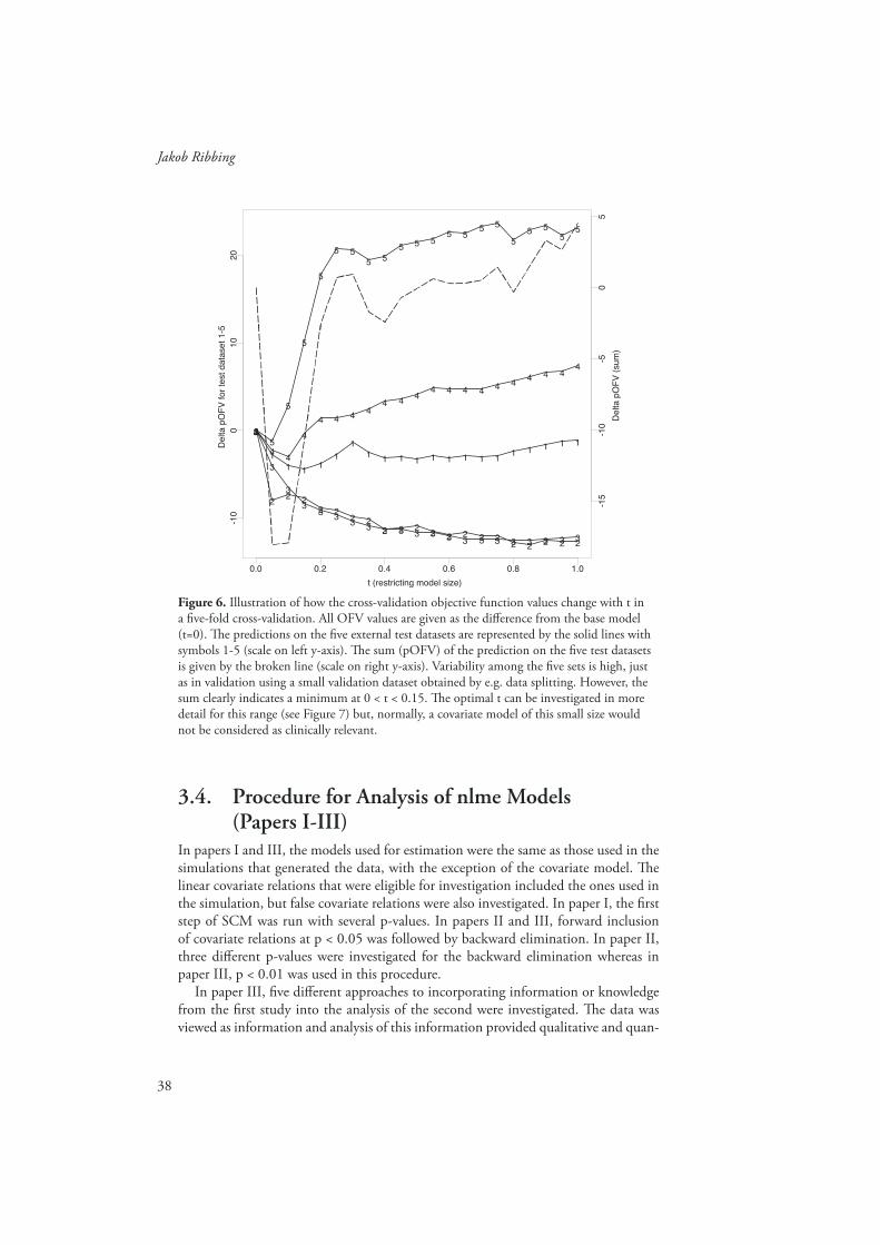
38

Jakob Ribbing

Figure 6. Illustration of how the cross-validation objective function values change with t in a fi ve-fold cross-validation. All OFV values are given as the diff erence from the base model (t=0). Th e predictions on the fi ve external test datasets are represented by the solid lines with symbols 1-5 (scale on left y-axis). Th e sum (pOFV) of the prediction on the fi ve test datasets is given by the broken line (scale on right y-axis). Variability among the fi ve sets is high, just as in validation using a small validation dataset obtained by e.g. data splitting. However, the sum clearly indicates a minimum at 0 < t < 0.15. Th e optimal t can be investigated in more detail for this range (see Figure 7) but, normally, a covariate model of this small size would not be considered as clinically relevant.

0.0 0.2 0.4 0.6 0.8 1.0

-10

010

20

12345

1

2

3

45

1

23

4

5

1

23

4

5

1

23

4

5

1

23

4

5

1

23

4

5

1

23

4

5

1

23

4

5

1

23

4

5

1

23

4

5

1

23

4

5

1

23

4

5

1

23

4

5

1

23

4

5

1

23

4

5

1

23

4

5

1

23

4

5

1

23

4

5

1

23

4

5

1

23

4

5D

elta

pO

FV

for

test

dat

aset

1-5

t (restricting model size)

-15

-10

-50

Del

ta p

OF

V (

sum

)

5

3.4. Procedure for Analysis of nlme Models (Papers I-III)

In papers I and III, the models used for estimation were the same as those used in the simulations that generated the data, with the exception of the covariate model. Th e linear covariate relations that were eligible for investigation included the ones used in the simulation, but false covariate relations were also investigated. In paper I, the fi rst step of SCM was run with several p-values. In papers II and III, forward inclusion of covariate relations at p < 0.05 was followed by backward elimination. In paper II, three diff erent p-values were investigated for the backward elimination whereas in paper III, p < 0.01 was used in this procedure.

In paper III, fi ve diff erent approaches to incorporating information or knowledge from the fi rst study into the analysis of the second were investigated. Th e data was viewed as information and analysis of this information provided qualitative and quan-

39


Figure 7. Illustration of the covariate model using a fi ner grid in the relevant range of t-values. Th e predictive objective function value (pOFV) is represented by the broken line and the scale on right y-axis. It has its minimum at t=0.06. At this t, two covariate relations are selected by the lasso: CLCAGE and VHCTZ0. Th e former denotes the eff ect on CL of age above 60 (otherwise zero, as defi ned in the original publication14) and the latter the eff ect on V of having no concomitant treatment with hydrochlorothiazide; the typical subject was on this treatment. Covariate relations that are not included in the lasso model for any of the investigated t-values are not plotted in the graph, but all the 20 investigated covariate rela-tions are presented in the legend (to the right).

t (restricting model size)0.0 0.05 0.10 0.15

-0.0

6-0

.04

-0.0

20.

00.

020.

04

1

1

1 1

1

1

1

1

11 1 1

11 1

10 10 10 10 10 10 10 10 10 10

1010

1010 10

12 12 12 12 12 12 12 12 12 12 12

1212

12 12

14 14 14

14

14

14

14

14

14

14

14 14 14 14 14

18 18 18 18 18 18 18 18 18 18

1818 18 18

18

Cov

aria

te c

oeffi

cien

t ope

ratin

g on

sta

ndar

dize

d co

varia

te

-15

-10

-50

Del

ta p

OF

V (

sum

)

SYMBOL COEFF

123456789

1011121314151617181920

CLCAGECLCHTCLCON0CLHCT0CLPRO1CLRAC2CLSECRCLSEX2CLSMO1CLWTVCAGEVCHTVCON0VHCTZ0VPROP1VRACE2VSECRVSEX2VSMOK1VWT

Delta pOFVCut-off limit

titative knowledge in the form of an nlme model. Th e fi ve approaches to knowledge propagation were: analysing the studies after pooling them into one dataset (DP), merging the results after analysing the studies separately (MM), fi tting a pre-specifi ed model that was selected from a previous study on either the most recent study (PS) or on the pooled dataset (PSP), and naïvely analysing the most recent study (NI) with-out taking into account the results of analysing any previous study.

In paper II, SCM and the lasso were compared on datasets of diff erent sizes, i.e. including diff erent numbers of subjects. Th e comparisons were made according to diff erent scenarios, including two diff erent base models and either only investigat-ing linear models or additionally investigating piece-wise linear models, cf. Equation (13). Th e base models were both parsimonious models identifi ed on the large original dataset23 whereas the stochastic model was slightly simplifi ed for better estimability on small datasets. Reasonable simplifi cations were identifi ed by the use of bootstrap-ping with a small sample size.116, 117 Th e two basic models were identical except that one was a basic model without any covariates and the other was an allometric model based on body weight and calculated fat-free mass.76, 118, 119

40

Jakob Ribbing

3.5. Development of a Model for FPG and FI (Paper IV)

Topp et al. proposed a model for BCM, (fasting) insulin and glucose dynamics in normal subjects.104 Th e structure of this mechanistic model was used as the starting point for the current analysis, and components for treatment and disease progres-sion120 in diff erent groups of patients were added. Topp et al. presented mean values for the parameters for healthy individuals. However, it is likely that several of these will be changed in patients with diabetes. In the available data, fi ve diff erent disease groups (DGR) were defi ned as subjects in SIR (DGR 1), naïve and pre-treated GLAD patients (DGR 2 and 4, respectively) and naïve and pre-treated GALLANT6 patients (DGR 3 and 5, respectively). Th ese DGR can at least partly be ordered into diff erent disease stages120 as described in Figure 8. Further, a population approach was applied to the modelling to account for the heterogeneity between patients within the same DGR.

1 - SIR

Non-diabetic but withreduced insulin sensitivity

2 - GLAD

Naïve diabetics in theGLAD study

3 - GALLANT

Naïve diabetics in theGALLANT-6 study

0 - HV

Healthy volunteers. Nodata, only literature

4 - GLAD

Pre-treated diabetics inthe GLAD study

5 - GALLANT

Pre-treated diabetics inthe GALLANT-6 study

?

?

?

?

Figure 8. Illustration of the disease stage in healthy volunteers and the fi ve diff erent disease groups (DGR). Th e typical drug-naïve patients in the SIR, GLAD and GALLANT6 studies can be assumed to have an increasing degree of diabetes. However, it is not obvious how to rank the pre-treated patients in relation to the drug naïve in the same study.

Topp et al. described the net changes for FPG, FI and BCM in three diff erential equa-tions. All parameters in these equations cannot be identifi ed from the data available in this work. Th erefore, disease progression was described as a change from the healthy state in two parameters which were estimated separately for each of the fi ve DGR. Th e fi rst parameter was insulin sensitivity (S). Reduced insulin sensitivity alone does not cause diabetes, since beta-cell adaptation acts as a negative feedback to eventually bring the FPG back to the set-point. Th e second parameter (OFFSET) off set beta-cell adaptation so that this strove towards a higher set-point FPG. Th is eff ectively reduced

41


the BCM as the OFFSET increased. Th e rate of beta-cell adaptation at diff erent FPG levels is illustrated for a healthy and an off set (i.e. type 2 diabetic) individual in Figure 9.

5 10 15 20

64

20

FPG (mmol/l)

dBC

M/d

t (%

/day

)

Figure 9. Beta-cell adaptation rate versus FPG. Th e grey curve represents the change in a healthy individual and the black in an off set (diabetic) individual. At higher FPG values the two curves join at a high (positive) adaptation rate. Th e dotted vertical lines mark the physi-ological fi xed points in each of the two individuals. Th is is a point of attraction and the beta-cell adaptation acts with a negative feedback to bring the FPG back to this point.

Th e initial modelling attempts were not successful in describing the treatment eff ects because a higher decline in FI than expected from the decline in FPG was seen. A relation between insulin elimination and insulin sensitivity95, 96 was therefore incor-porated into the model. Treatment eff ects were incorporated directly on OFFSET where the eff ect delay was accounted for by beta-cell adaptation but as an indirect eff ect on insulin sensitivity. Diff erences in the degree of disease for diff erent DGR were included in the model. However, since none of the studies lasted longer than six months, no attempt was made to identify individual disease progression during the study period. Th e adaptation of BCM is seen as a symptomatic eff ect of treatment, much like the eff ect on insulin sensitivity. Th ese should be separated from any under-lying disease progression in OFFSET and S. Finally, the fact that only fasting observa-tions of glucose and insulin were available allowed the assumption that these variables were at steady state with respect to each other, given the current level of BCM and insulin sensitivity. Th e interdependencies between the diff erent variables in the model are illustrated in Figure 10.

42

Jakob Ribbing

Figure 10. Schematic illustration of the FPG-FI model. Changes from the steady state are illustrated as indirect eff ects for all four variables, indicated by solid or broken arrows. How-ever, responses in FPG and FI are relatively fast and therefore assumed at steady state relative to one another, at the given level of S and BCM, indicated by the broken arrows. Drug treat-ment exerts an indirect eff ect on S and BCM which explains the delay in the response on FI and FPG. Th e indirect eff ect of drug treatment and the eff ect of S on the elimination of FI are additions to the model as originally suggested by Topp et al.

3.6. Adaptive Learning (Paper III)In the scenario where the optimal design was used, the second study was performed with an ED optimal design.112 Th is was based on the knowledge gained from analys-ing the fi rst study and on the knowledge on the distribution of the covariate values in the patient population. Th e number of observations per subject in the second study was substantially lower than in the default scenario but the number of subjects was the same. Th e study was optimized on the observation times as well as on which indi-viduals to include (stratifi cation).

Special subpopulations are often investigated to rule out the possibility that a covariate is clinically relevant or to confi rm the fi ndings of a previous study.9, 121, 122 However, here design optimization was performed using the full-forward covariate model obtained from analysing the fi rst study. Th erefore, only the subpopulations representing the covariates which were in the fi rst model were eligible for stratifi ca-tion. An error model assuming proportional error distribution was used, cf. Equation

BCM

FPG

FI

-

+

++

S+

+

+

+Pre-

treatment ortesaglitazarexposure

43


(5) which also assumes the same proportional error magnitude during the absorption and elimination phases. Because of this, the sample times were restricted to the same interval as for the non-optimized designs (0.2-4 typical half-lives of the drug).

To account for uncertainty in both the individual covariate values and the param-eter estimates, a modifi ed ED optimization was performed. It was modifi ed in the sense that both the model parameters and the model covariates were assumed to have a distribution associated with them.

3.7. Calculation of Power and Inclusion Rates (Papers I and III)

Th e inclusion rate was calculated for each scenario and for each covariate relation as the percentage of the replicates from which the covariate was selected. Since the data were generated by simulation from a model in papers I and III, the true covariates and those that were only correlated with (or unrelated to) the parameter were known. Because of this, we used the term power in paper I. Power is the percentage of replicate datasets from which all true covariates were selected. In this paper there was only one true covariate.

3.8. Evaluation of Selection Bias (Papers I and III)Bias denotes the presence of a systematic error causing the expected value (averaged over many repeats) to deviate from the true value. Th e (conditional) selection bias can only be calculated from the replicates where all true covariates were selected, because it is otherwise confounded with omission bias.83 Th is has two implications. Th e fi rst is that selection bias is best calculated from repeated analyses of simulated data, as it is otherwise not known which covariates are true. Th e second is that the calculation of selection bias may require analysis of a large number of replicates if the power of fi nding all true covariate relations is low. Th is was the reason for the high number of replicates used in papers I and III. Selection bias was calculated on a relative scale according to

Nrepl

cov cov

1 covcov #

1

ˆ( )

100%

nP Pn

n PP replicates

nn

sSelection bias

s (19)

where sn equals one if all true covariates were selected and zero otherwise, nPcov is the estimated covariate coeffi cient for parameter P and covariate cov from dataset replicate n, and Pcov is the covariate coeffi cient cov without selection bias. In paper III, Pcov was calculated as the average estimate over all replicates when estimating the true covari-ate model. In paper I, the value used in simulation was used. Th ere is no diff erence between these two approaches unless the estimation method provides biased estimates (estimation bias).

44

Jakob Ribbing

3.9. Evaluation of Predictive Performance (Papers I-III)

Th e predictive performance was used to summarize how well a model can predict new data or some aspect of it. In paper I, the model error of the true covariate parameter was calculated for the replicates where the covariate was statistically signifi cant; this is the same as being selected if we let no other covariates compete for selection. Th is approach was taken since the initial investigation showed that selection bias was not much infl ated due to competition. Th e model error was calculated on a relative scale as the mean absolute error (mae) according to

cov cov

1 covcov

1

ˆrepl

replicates

N

nP Pn

n PP N

nn

s

mae

s(20)

where Nrepl equals 7 400 and the remaining notation is as explained in subsection 3.8 above.

In paper II, the prediction error was evaluated on the observations of the depen-dent variable (y) in the external validation datasets according to:

(21)

Where for validation dataset v, Ntot,v and Nsubj,v are the total number of observations and the number of subjects, respectively. For subject i in validation dataset v, Nobs,iv is the number of observations and yijv and yijv are the jth observation and prediction, respectively. Th e number of replicates (Nrepl) for each of 16 scenarios in this paper was 100.

In paper III, the model error was calculated on the estimated typical value of clear-ance as the root mean squared error

, ,

1 1,

1 1ˆ 100%

repl subj v obs ivN N N

DV ijv ijv ijvv i jrepl tot v

mae y y yN N

2

1 1

100% 1

min ,

replN Nsubjin in

TVCLn irepl subj in in

TVCL TVCLrmse

N N TVCL TVCL (22)

where TVCLin and TVCLin are the true and predicted TVCL values for individual i in replicate n, respectively. Th e min function in the denominator returns the smallest of TVCLin and TVCLin.

3.10. Evaluation of Design Optimization (Paper III)In addition to bias and predictive performance, the performance of the optimized and sparse design was compared with that of the default design by assessing the distribu-tions of the relative estimation error according to

45


(23)

where k is the true parameter value and nk and REEnk are the estimate and estima-tion error for parameter k in replicate n, respectively. Th e distribution of the relative estimation error was used to assess the estimation bias and precision of all parameters when the true model was fi tted to the second study.

Further, each optimal design calculation provided not only a design but also an estimate of the lower boundary of the parameter precision that would result if the optimized design would be realized and used as the only information source.123 Although not in the primary scope of paper III, these estimates were also evaluated. Th e estimate of the coeffi cient of variation for each parameter (CVnk) was compared to REEnk when the same model used to optimize the design was re-estimated using the second study with the realized optimal design. If CVnk were to be unbiased, the ratio of REEnk and CVnk would be distributed according to the standard normal distribu-tion, given that parameter estimates are normally distributed around the true value.

3.11. Evaluation of the Model for FPG and FI (Paper IV)

In paper IV, the capability of the model to describe the biomarkers without any (clini-cally) relevant misfi t was evaluated graphically. Th us, the model was evaluated by a visual predictive check64 (VPC) that included both the median profi le over time and the distribution of observations around the median. Th e 95% prediction interval (95%-PI; i.e. the 95%-confi dence interval predicted by the model) was included in the graphs. Th e results were displayed separated for diff erent subgroups, i.e. DSG and dose groups. In the VPC, simulations from the model were compared with the distribution that was actually observed at diff erent points in time and in diff erent subgroups. Th is was an internal evaluation. As an external evaluation of the model, the model predicted BCM in the diff erent DSG and the relations between insulin sensitivity and insulin elimination were compared with reports from the literature.

ˆ100%nk k

nkk

REE

46

Jakob Ribbing

4. Results

4.1. Power and Inclusion Rates (Papers I and III)Paper I describes the power, selection bias, and predictive performance in covariate modelling. Figure 11 displays the power of selecting the true covariate and the type-I error rate when covariate 1 was tested without competition from the other false covariates. Th e default simulations cover a wide range, from low to high power, and the type-I error rate is only slightly higher than the nominal value. Figure 12 depicts the relative change in the power of fi nding the true covariate when one of the false covariates was allowed to compete for selection. Th e selection was more resistant to correlation between the covariates when the dataset was large or when the true covari-ate coeffi cient was large, i.e. when a strong covariate eff ect was present in the investi-gated population.

0.0

0.2

0.4

0.6

0.8

1.0

0 200 400 600 800 1000

NN N

W

W

W

W

W

M

M

M

M M

S

S S S S

Numberof subjects

Po

we

rw

itho

ut

com

pe

titio

n

Figure 11. Th e power of selecting the true covariate without competition is shown for diff er-ent dataset sizes. Selection was made if p < 0.05 on datasets that were simulated with a covari-ate coeffi cient exerting a strong (S), moderate (M) or weak (W) infl uence on CL. Th e dotted horizontal line is drawn at the nominal signifi cance level, 0.05. Th e actual signifi cance level represented by simulation from the null hypothesis (N) is shown for small datasets (20, 50 and 100 subjects).

47


0.5

0.6

0.7

0.8

0.9

1.0

0.0 0.4 0.8

Weak c ovp < 0.001

1 1

1

1

2 2 2

2

3 3 3

3

4 4 4

4

5 5 5

5

Moderate c ovp < 0.001

1 1 1

1

2 2 2

2

3 3 3

3

4 4 4

4

5 5 5 5

0.0 0.4 0.8

Strong covp < 0.001

1 1 1

1

2 2 2

2

3 3 33

4 4 4 45 5 5 5

Weak c ovp < 0.01

1 1

1

1

2 2 2

2

3 33

3

4 44

4

5 5 5

5


1 11

1

2 22

2

3 33

3

4 4 4

4

5 5 5 5

0.5

0.6

0.7

0.8

0.9

1.0Strong cov

p < 0.01

1 11

1

2 2 2

2

3 3 33

4 4 4 45 5 5 5

0.5

0.6

0.7

0.8

0.9

1.0Weak c ovp < 0.05

1 1

1

1

2 2

2

2

3 33

3

4 44

4

5 5 5

5

0.0 0.4 0.8


1 1

1

1

2 22

2

3 33

3

4 4 4

4

5 5 5 5Strong cov

p < 0.05

1 11

1

2 2 2

2

3 3 33

4 4 4 45 5 5 5

Correlation between competing and true covariate

Rel

ativ

epo

wer

with

com

petit

ion

Plotting character: 1 2 3 4 5Number of subjects: 20 50 100 300 1000

Figure 12. Th e relative power of selecting the true covariate vs. correlation with the compet-ing covariate. Th e relative power is the ratio of power values with and without competition from a false covariate. Results are from one of many simulation set-ups and given for diff erent dataset sizes and a weak (left column), moderate (middle column) and strong (right column) covariate. Th e relative power is given for p < 0.05, 0.01 and 0.001 in the top, middle and bottom rows, respectively. As expected, weak covariates and small datasets made the selection less resistant to correlation (left column compared to right column and plotting character 1 compared to plotting character 5). Also, a stricter p-value made the selection more resistant to correlation (top row compared to bottom row).

Paper III describes knowledge propagation in model-based analyses. Th e inclusion rates of all six investigated covariates are shown in Figure 13 for the diff erent simula-tion scenarios and knowledge propagation approaches. Th e false covariates are easily identifi ed since their inclusion rates are much lower. Th e diff erent covariates in this comparison can be said to compete for selection. However, for SEX and WT there is actually a synergy in the selection. Th ese covariates mask the eff ect of each other and selection of one encourages selection of the other. Not surprisingly, pooling all available data is superior for identifying the true covariates. However, this may also encourage inclusion of false (but correlated) covariates to a higher extent. From a qualitative perspective, the merge approach to knowledge propagation is more inclu-sive than other approaches.

48

Jakob Ribbing

Figure 13. Inclusion rate for the diff erent approaches to knowledge propagation, given simu-lation set-up and covariate. Both pre-specifi ed approaches (PS & PSP) result in the same qualitative estimation of knowledge and are therefore not separated in this fi gure. Th e actual approaches are symbolized by white bars. For the Model Merge (MM) approach, if a covariate was selected from both the fi rst and the second study, this is symbolised by an overlaid black bar. Analysing the pooled dataset (DP) provides the highest inclusion rate of the true covari-ates. Th e MM approach is more inclusive than the approaches selecting the model from either the fi rst or the second study (NI, PS, and PSP).

4.2. Selection Bias (Papers I and III)For paper I, Figure 14 shows the selection bias in the true covariate coeffi cient when the true covariate was investigated alone or in competition with the four false covari-ates. Th e selection bias was very high (>100%) when a weak covariate relation was selected from a small dataset ( 50 individuals). Surprisingly, however, competition of false covariates added little to the selection bias when statistical signifi cance was required. Th is can be seen in that the selection bias in the left panel column was only marginally higher than that in the right column. Focusing only on the selection bias without competition and using the results from all available scenarios and covariates, Figure 15 shows that without competition the selection bias was a function of the power. If the power was less than 20% when using a p-value of 0.05 or stricter, the bias was more than 100%. Th is means that the identifi ed covariate relation can be expected to worsen (external) predictions from the model. Further, evaluating the importance of the biased covariate coeffi cient may falsely lead to the conclusion that

DP

MM

PS & PSP

NI

10 40 70 100

AGEDefault

ATARDefault

10 40 70 100

C2E1Default

CRCLDefault

10 40 70 100

SEXDefault

WTDefault

DP

MM

PS & PSP

NI

AGEOptimal-Sparse Design

ATAROptimal-Sparse Design

C2E1Optimal-Sparse Design

CRCLOptimal-Sparse Design

SEXOptimal-Sparse Design

WTOptimal-Sparse Design

DP

MM

PS & PSP

NI

AGESmall Second Study

ATARSmall Second Study

C2E1Small Second Study

CRCLSmall Second Study

SEXSmall Second Study

WTSmall Second Study

DP

MM

PS & PSP

NI

AGESingle Strong Small Second

ATARSingle Strong Small Second

C2E1Single Strong Small Second

CRCLSingle Strong Small Second

SEXSingle Strong Small Second

WTSingle Strong Small Second

DP

MM

PS & PSP

NI

AGESingle True Covariate

10 40 70 100

ATARSingle True Covariate

C2E1Single True Covariate

10 40 70 100

CRCLSingle True Covariate

SEXSingle True Covariate

10 40 70 100

WTSingle True Covariate

Kno

wle

dge

prop

agat

ion

met

hod

AGEDefault

ATARDefault

C2E1Default

CRCLDefault

SEXDefault

WTDefault

AGEOptimal-Sparse Design



CRCLOptimal-Sparse Design



AGESmall Second Study



CRCLSmall Second Study



AGESingle Strong Small Second



CRCLSingle Strong Small Second



Inclusion rate (%)

49


this is a clinically relevant relation. Attempts to assess the power from the biased esti-mate would result in an overestimation.

0

50

100

150

200

250

300

0 200 400 600 800

All 4 fals e competingp < 0.001

W

W

W

W

W

M

M

MM M

SS S S S

Without Competitionp < 0.001

W

W

W

W

W

M

M

MMM

SS S S S


W

W

W

WW

M

M

MM M

SS S S S 0

50

100

150

200

250

300Without Competition

p < 0.01

W

W

W

WW

M

M

MM M

SS S S S

0

50

100

150

200

250

300


W

W

W

WW

M

MM M M

SS S SS

0 200 400 600 800

Without Competitionp < 0.05

W

W

W

WW

M

MM M MSS SSS

Number of subjects

Bia

s(%

)

Covariate Strength

W WeakM ModerateS Strong

Figure 14. Selection bias in a true covariate coeffi cient vs. dataset size. Results were derived from one of many simulation set-ups and given for a weak (W), moderate (M) and strong (S) covariate. Th e bias is given for p < 0.05, 0.01 and 0.001 in the top, middle and bottom rows, respectively. In the left column, the true covariate model has been selected in competi-tion with the four false covariates whereas, in the right column, no competing covariate has been allowed to aff ect selection. As can be seen, the selection bias is severe for weak covariates selected from small datasets. Th e selection bias caused by requiring statistical signifi cance is not increased much by competition from the four false covariates (left column compared to right). Also, as can be expected, the requirement for a stricter p-value increases the selection bias (top row compared to bottom row).

50

Jakob Ribbing

0

100

200

300

400

0.0 0.2 0.4 0.6 0.8 1.0

p < 0.001

A

A

A

A

A

B

B

B

C

C

CD

D

D

EE

E

F

F

F

G

G

H

H

A

A

A

A

A

A

A

A

A

A

A

A

A

A

A

A

A

A

A

B

B

B

B

C C

C

DD

D

EE

E

F

F

F

F

G

G

G

G H

H

H HA

A

A

A

A

A

A A

A

AA A

A

A AA

A

AA

0

100

200

300

400p < 0.01

AA

A

A

A

A

A

A

A

A

A

A

AA

B

B

B

B

CC

C

D

D

D

E

E

E

F

F

F

G

G

G

HH

H

A

A

A

A

A

A

A

A

AA

A

AA

A

A

A

A

A

A

A A

A

BB

B

BC

C

CD

D

DD

E

EE F

F

FFG

G

GH

H

H

H A

A

AAA

A

AAAA

AA

0

100

200

300

400p < 0.05

A

A

A

A

A

A

A

A

A

A

A

A

A

A

AA

A

A

A

A

AB

B

B

B

C

C

C

D

D

D

E

E

E

FF

F

GG

G

H

H

H

A

A

AA

A

A

A A

A

A A

A

A

A

A

A

A

A

A A

A

A

AB

B

B

BC

C

C

CD

D

D

DE

E

E EF

F

FFG

G

G

GH

H

HH A

A

A AA

A

AAAA AA

Power without competition

Bia

s(%

)

Figure 15. Bias in the estimated covariate coeffi cient vs. power. Results are derived from dif-ferent scenarios (plotting characters A-H) given p < 0.05, 0.01 and 0.001 in the top, middle and bottom rows, respectively.

In paper III, where bias was only investigated in the presence of competition, two more aspects of selection bias can be seen (Figure 16). Th e fi rst is that unevenly dis-tributed covariates (e.g. ATAR) require larger datasets. Th is is because such covariates are less informative.79 Th e other aspect is that the masking covariates (SEX and WT), which often end up in the model together, infl ate the selection biases of each other. Th is is due to correlations of estimate, or colinearity.70 If the correlation is not pre-served, e.g. in another patient population, predictions from this model would perform particularly poorly. Further, the two covariates may falsely be regarded as clinically rel-evant due to the bias. Th e two may seem clinically relevant if assessing each covariate separately even though the contributions from the two covariates in combination are modest in most individuals. Regarding the performance of the diff erent approaches to knowledge propagation, the naïve-independent approach resulted in very high selec-tion bias. Th e pre-specifi ed approach was unbiased, the merge approach was almost so, whereas the remaining two approaches were in-between.

51


Figure 16. Selection bias in the estimated covariate coeffi cient for the “true” covariates in the diff erent simulation set-ups. To indicate uncertainty, an 80% confi dence interval has been drawn as a horizontal line wherever the line expands outside the dot marking the point estimate of bias. As was expected, the Pre-Specifi ed (PS) approach had no selection bias. Th e Data-Pool (DP) approach shows a moderate selection bias in most set-ups. Th e Naïve-Independent (NI) approach, however, shows severe selection bias in the estimated eff ects of ATAR, WT and in all four covariates with the Small Second Study. Th e Pre-Specifi ed-Data Pool (PSP) had a selection bias which was between those of the NI and the PS approaches. Th is is seen from the two simulation set-ups where this approach has been evaluated, in the two lowest panels. Th e Model-Merge (MM) approach had low selection bias.

4.3. Predictive Performance (Papers I-III)For paper I, Figure 17 shows that the predictive performance is a function of power without competition. Covariate relations selected at p < 0.05 with a power < 25% reduce the predictive performance compared to the null hypothesis of no covariate eff ect.

DP

MM

PSPPS

NI

0 50 100 200

ATARDefault

C2E1Default

0 50 100 200

SEXDefault

WTDefault

DP

MM

PSP

PS

NI





DP

MM

PSP

PS

NI





DP

MM

PSP

PS

NI





DP

MM

PSP

PS

NI

ATARSingle True Covariate

0 50 100 200

C2E1Single True Covariate

SEXSingle True Covariate

0 50 100 200

WTSingle True Covariate

Selection Bias (%)

Kno

wle

dge

prop

agat

ion

met

hod

52

Jakob Ribbing

Figure 17. Graph showing log mae of the estimated covariate coeffi cient vs. power. Results were derived from diff erent simulation scenarios (plotting characters A-H), given p < 0.05, 0.01 and 0.001 in the top, middle and bottom rows, respectively. Th e dotted vertical and horizontal lines intersect at the point where the selected covariate model is expected to have no infl uence on the predictive performance. Th is point was estimated using the Splus-super smoother.109 Th e lower right quadrant represents the high powered covariates which are expected to improve the predictive performance. Th e upper left quadrant represents low-pow-ered covariates expected to worsen the predictive performance.

For paper III, Figure 18 displays the predictive performance for the diff erent approaches to knowledge propagation and for diff erent scenarios. Th e pooled analysis performed the best in all scenarios. Th e naïve-independent analysis of the second dataset alone was the worst. When the second dataset was small (50 individuals), this approach performed worse than the base model. Fitting a pre-specifi ed model to the pooled dataset was better than the unbiased alternative of only fi tting the second study. Th e optimal design performed about as well as the empirical less sparse design. Th ese are further compared to the default scenario in subsection 4.5.

-1.5

-1.0

-0.5

0.0

0.5

1.0

0.0 0.2 0.4 0.6 0.8 1.0

p < 0.001

AA

A

A

A

B

B

B

C

C

C

D

D

DE

E

EF

F

FGGHH

A

A

A

A

A

A

A

A

A

A

A

A

A

A

A

A

A

A

A

B

B

B

B

C

C

C

D

D

DE

E

E

F

F

F

FG

G

G

G

H

H

H

H

A

A

A

A

A

A

AA

A

A

A

A

A

A

A

A

A

A

A

A

A

A

A

A

A

A

A

-1.5

-1.0

-0.5

0.0

0.5

1.0p < 0.01

A

A

A

A

A

A

B

B

B

B

C

C

C

D

D

DE

E

EF

F

FG

G

G

H

H

H

A

A

A

A

A

A

A

A

A

A

A

A

A

A

A

A

A

A

A

A

A

A

B

B

B

B

C

C

C

D

D

D

DE

E

E

F

F

F

FG

G

G

H

H

H

H

A

A

A

A

A

A

A

A

A

A

A

A

A

A

AA

A

A

A

A

A

A

A

A

A

A

A

-1.5

-1.0

-0.5

0.0

0.5

1.0p < 0.05

A

A

A

A

A

A

B

B

B

B

C

C

C

D

D

DE

E

E

F

F

FG

G

G

H

H

H

A

A

A

A

A

A

A

A

A

A

AA

A

A

A

A

A

A

A

A

A

A

A

B

B

BB

C

C

C

C

D

D

D

D E

E

E

EF

F

F

FG

G

G

GH

H

H

H

A

A

AA

A

A

A

A

A

A

A

A

A

A

A

A

A

A

A

A

A

A

A

A

A

A

A

A

Power without competition

log

mae

53


Figure 18. Root mean squared error (rmse) in the estimated typical values of clearance pro-vided for the diff erent approaches and diff erent simulation set-ups. As references, two models without data-driven model selection are included: the True and the Basic covariate models fi tted to the second dataset are represented by the broken and dotted lines, respectively. Despite the selection bias when using the Data Pool (DP) (cf. Figure 16), this approach is superior not only to the Naïve-Independent (NI) approach but also to the Pre-Specifi ed approaches (PS and PSP). Th e PS performed better than the NI in all set-ups and especially for the Small Second Study set-ups where better prior information on which covariates are important were available from the fi rst study. Where investigated, the Pre-Specifi ed Data Pool (PSP) predicted better than the PS. Th is could be expected since the pre-specifi ed model selection was not excessively data-driven. Th e x-axis is cut on the left side at the lowest pos-sible rmse in any of the simulation set-ups (obtained by fi tting the true covariate model to the pooled dataset).

For paper II, Figure 19 displays the prediction error for SCM with three diff erent p-values. For predictive-covariate modelling, the optimal p-value for selection was not primarily dependent on the number of covariate relations investigated. Rather it depended on the information content in the data on the investigated relations, i.e. the signal-to-noise ratio. Since, for these data, the allometric model explained much of the variability that could be explained by the collected covariates, the investigated covariates mainly contributed with noise. Any covariate investigation starting from the allometric base model was best performed with a strict criterion, i.e. a low p-value. Further, the results from the standard base model showed that dataset size (infl uenc-ing the signal-to-noise ratio) had an infl uence on the optimal p-value. In the small datasets with 40-60 subjects the signal could not be separated from the noise and the strictest p-value performed best. However, in the larger dataset with 120-180 subjects

DP

MM

PSP

PS

NI

6 8 10 12 14 16

Default

DP

MM

PSP

PS

NI

Optimal-Sparse Design

DP

MM

PSP

PS

NI

Small Second Study

DP

MM

PSP

PS

NI

Single Strong Small Second

DP

MM

PSP

PS

NI

Single True Covariate

Root Mean Squared Error in TVCL (%)

Kno

wle

dge

prop

agat

ion

met

hod

dotted lines =

broken lines = True Covariate Model

Basic Model

54

Jakob Ribbing

the strictest p-value performed worst.

Dataset size (number of subjects)

mae

(%

)

46

48

50

52

40 60 120 180

Linear + Piece wise linearStandard

LinearStandard

Linear + Piece wise linearAllometric

40 60 120 180

46

48

50

52

LinearAllometric

SCM p<0.001SCM p<0.01SCM p<0.05

Figure 19. Th e mean absolute prediction error (mae) for SCM with three diff erent p-values, investigated in 16 scenarios. Each scenario was a combination of four diff erent analysis data-set sizes (x-axis), two diff erent starting models (allometric or standard) and two diff erent sets of investigated covariate relations (only linear or additionally piece-wise linear). Th e optimal p-value resulting in the best predictive performance (i.e. low mae), was dependent on the number of investigated covariate relations, but more importantly on the signal-to-noise ratio. Since the allometric model (top panel row) accounted for most of the variability that can be explained by the covariates, a conservative (low) p-value performed best for these scenarios. However, with the standard starting model (bottom panel row) the optimal p-value was dependent on the dataset size. For the very small datasets (40 subjects), the strictest p-value performed the best whereas for larger datasets (120-180 subjects) this p-value performed the worst. For comparison to the lasso later in this work, SCM was represented by the model that used the optimal p-value for each scenario, i.e. diff erent p-values for diff erent scenarios.

In Figure 20, SCM is compared with the lasso and the base model. In this graph, SCM is represented by the p-value that performed best in each scenario. Still, SCM performed worse than the base model in the small datasets. In all 16 scenarios, the lasso performed better than the base model and SCM with any of the three p-values. However, the diff erences between the lasso and SCM were very small for the large datasets when the optimal p-value was used.

55


Figure 20. Th e mean absolute prediction errors (mae) for the base model, the lasso, and the optimal SCM model (SCMoptimal) were compared in the 16 scenarios. “SCMoptimal” denotes SCM with the p-value that performed best in each scenario. Even so, for small datasets with 40-60 subjects SCM performed worse than the base model, i.e. no covariate investigation at all. Th e lasso, on the other hand, performed best in all 16 scenarios: better than the base model and SCM with any of the three p-values. However, the diff erences were small when the allometric model was used (top panel row). Th is was because the investigated covariates did not explain much variability that was not already accounted for by the base model. Further, also because the optimal P-value was used for SCM. Also, for large datasets with the standard base model as starting point for the covariate analysis (bottom panel row) the diff erence was small between SCM and the lasso.

Figure 21 shows that lasso cross-validation provided a nearly unbiased estimate of the prediction error. SCM, which used all analysis data to develop the model, provided only an apparent prediction error which was overly optimistic, i.e. biased low.


mae

(%

)

46

48

50

52

40 60 120 180

++

+ +

o

o

oo

x

x

xx

Linear + Piece wise linearStandard

++

+ +

o

o

oo

x

x

xx

LinearStandard

++

+ +

oo

o o

xx

x x

Linear + Piece wise linearAllometric

40 60 120 180

46

48

50

52

++

+ +

oo

o o

xx

x x

LinearAllometric

+ + +o o ox x x

base modellassoSCM optimal

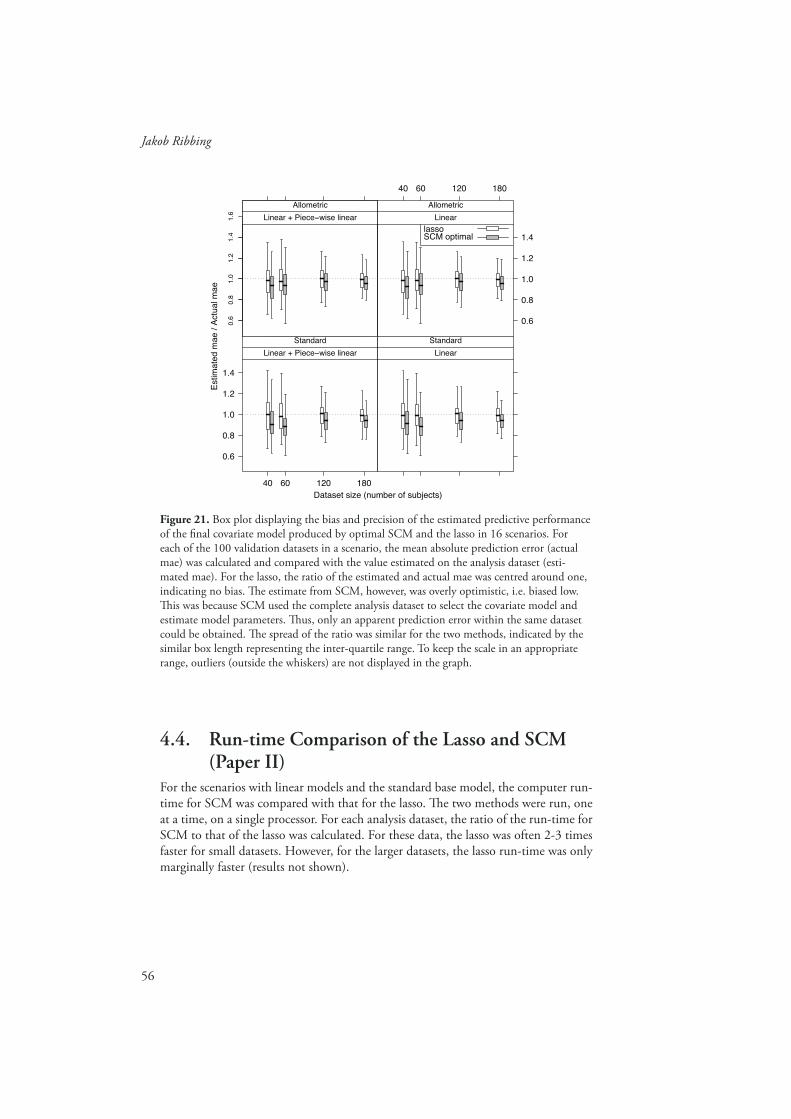
56

Jakob Ribbing

Figure 21. Box plot displaying the bias and precision of the estimated predictive performance of the fi nal covariate model produced by optimal SCM and the lasso in 16 scenarios. For each of the 100 validation datasets in a scenario, the mean absolute prediction error (actual mae) was calculated and compared with the value estimated on the analysis dataset (esti-mated mae). For the lasso, the ratio of the estimated and actual mae was centred around one, indicating no bias. Th e estimate from SCM, however, was overly optimistic, i.e. biased low. Th is was because SCM used the complete analysis dataset to select the covariate model and estimate model parameters. Th us, only an apparent prediction error within the same dataset could be obtained. Th e spread of the ratio was similar for the two methods, indicated by the similar box length representing the inter-quartile range. To keep the scale in an appropriate range, outliers (outside the whiskers) are not displayed in the graph.

4.4. Run-time Comparison of the Lasso and SCM (Paper II)

For the scenarios with linear models and the standard base model, the computer run-time for SCM was compared with that for the lasso. Th e two methods were run, one at a time, on a single processor. For each analysis dataset, the ratio of the run-time for SCM to that of the lasso was calculated. For these data, the lasso was often 2-3 times faster for small datasets. However, for the larger datasets, the lasso run-time was only marginally faster (results not shown).

40 60 120 180

0.6

0.8

1.0

1.2

1.4

1.6

Allometric

Linear + Piece wise linear

40 60 120 180

0.6

0.8

1.0

1.2

1.4

Allometric

Linear

lassoSCM optimal

40 60 120 180

0.6

0.8

1.0

1.2

1.4

Standard

Linear + Piece wise linear

Standard

Linear

Est

imat

ed m

ae /

Act

ual m

ae


57


4.5. Design Optimization (Paper III)When analysing the realized optimal design the PopED estimate of parameter uncer-tainty seems to be very accurate (unbiased) for most parameters, as seen in Figure 22. As seen in Figure 23, the ratio of REE and CV followed the standard normal distri-bution (indicated by the grey broken line) for six of the eight parameters displayed. Th e REE used in this fi gure was calculated for the model that was used to optimize the design in each replicate and consequently a covariate parameter could only be evaluated if present in that model (which occurred in 23-59% of the replicates for the four true covariates). Th e two covariates with the lowest inclusion rates in Figure 13 also had the highest selection bias in Figure 16 (WT and ATAR). Th ey generally exhibited larger relative estimation errors than those estimated by PopED. Th is could be expected since the standard error of these parameters must be biased low55 while the magnitude of the estimated coeffi cients was biased high, both as a result of model selection.

Rel

ativ

e es

timat

ion

erro

r (%

)

Parameter

-200

-100

010

020

0

CL V ka ATAR C2E1 SEX WT IIV-CL IIV-V IIV-ka SIGMA

2. Optimal-Sparse Design

-200

-100

010

020

0

CL V ka ATAR C2E1 SEX WT IIV-CL IIV-V IIV-ka SIGMA

1. Default

Figure 22. Relative estimation error (REE) when estimating the true model using the second study in the Default simulation set-up and the Optimal Sparse Design set-up. Due to the sparseness of the design in the latter, some structural and variance parameters were estimated with slightly lower precision: SIGMA (i.e. ), IIV-ka, IIV-V, ka, and V. For the covariate parameters on the other hand, the sparseness was compensated for by the stratifi cation. Th erefore the parameter precision was unchanged or even improved e.g. as for ATAR, the covariate which had the most uneven distribution without stratifi cation. For both the Default and Optimal Sparse Designs there was a downward bias in IIV-CL. Further, in the Optimal Sparse Designs, IIV-ka was estimated with an upward bias at the expense of SIGMA which was estimated with a downward bias.

58

Jakob Ribbing

Figure 23. Quantile-quantile plot of the distribution of the z-score (the ratio of REE and PopED-estimated coeffi cient of variation) for the 1 000 estimates in the Optimal Sparse Design set-up. Th is ratio followed the standard normal distribution for most estimates (grey broken line). Th e covariate parameters for ATAR and WT showed a wider distribution of REEs than expected from the PopED estimates. Th is was probably due to the data-driven model selection causing both selection bias and seemingly too precise estimates of selected covariate eff ects. Th e parameters CL and IIV-CL were excluded from this fi gure since cal-culation of REE was not straight-forward for these: the references for these two parameters changed with the covariate model that was estimated in each replicate.

4.6. Diabetes Model (Paper IV)From paper IV, the VPC on the FPG data is presented in Figure 24, stratifi ed on both DGR and dose. Th e model described both the median and the 95% confi dence inter-val well. Any major discrepancies between the model-predicted and observed medians were probably due to too few observations; e.g. the 0.1 mg dose group in DGR 2, where the treatment eff ect appeared to be higher than that in the individuals in the same DGR treated with 0.5 or 1 mg. No clear trend was seen in the 95%-PI for dose groups or studies where the coverage was not appropriate. Th e VPC on the FI data is presented in Figure 25, stratifi ed on both DGR and dose. Th e model described both the median and the 95% confi dence intervals very well.

-10

-5

0

5

-3 -2 -1 0 1 2 3

IIV-V IIV-KA

-3 -2 -1 0 1 2 3

SEX WT

V

-3 -2 -1 0 1 2 3

KA ATAR

-10

-5

0

5

-3 -2 -1 0 1 2 3

C2E1

Unit normal quantile

z=R

EE

/Est

-CV

59


Figure 24. Visual predictive check of FPG on the new model developed on all three studies. Th e blue lines represent model predicted median and 95%-prediciton interval (PI). Th e black circles represent observations within the PI and the red numbers display the outlying ID numbers. Th e black line is a linear interpolation of all observations. Observations in DGR 5 are jittered in the horizontal direction for visibility since this group includes almost half of the total number of observations. Th e model describes the observed median and 95%-confi dence interval well.

510

15

0 mg tesaglitazar in DGR 1

1119 111911191119111911191207

13541357

191919 1911001118121112111232

13181363

0.1 mg tesaglitazar in DGR 1

1111111

1168 1168116811861260 1294

122712271314 13141314131413141314131413141314


148 148 12121226 1226

11061113 11941226 12345

1015


151

161161121513431369


1213 1228122812421242

1242124212421242

1196 119612281288


2902902112 211221122112

21122198

510

15


21342207 23062306

2306

2306

256 256 220722542279 2279


281281 28128128128422822282

228222822330

2390


218

218218

510

15


267 2151220122012201

2209

2732179


265265265

2652166 21662341 2341

2341

2312102 228922892317


247247 282282282

2165223022302230

2265233923392381

234 234 247 216121812308 23422352 23682373 237323732391 2391

510

15


222139 2233 2233230323452367

2367236723672375


21702251

23362372

25 233268

2205 2232


2512542154

222222372237

2268

22962296229622962307

2912132

510

15


22192293

22932293

22932365

236523652410

2102632632852852383


2171

2338

213121352180 22002220 22572257


612361606412 64126412

641264126632663266326632

66396639

6639

66406640

6640

6386123 61236124 61246124

630964266426 64266596

6641

66426644

50 0 50 100 150

510

15


614761476147614761476147

62166216

62846434 6470

50 0 50 100 150


618

658665 66561186127612761276127

6138613861386138615861646183

6183618361836183

618562096209

6214623662366237

6248 62726315 6315

6342

63436368 63686368

6368

63766376

64216421

6447

6474647764836496

65016501 65016501 6512

6517

6517

651765176543

6543

6547

65636563 656365636572

6588

6590 6590660266156625 66386670

615627676 676694 694696610261036112616361636167 616761676167616761676168

619062036231 6231623162316231 6231623162316253 625362666266629963206339

633963396339 63396339

63416342 637263766423 64236423642364236431 6431 64316442644264426455

649064976519651965196521 6521 65216525 65346535 65426559 6559 65596564 656465896594

66256626

50 0 50 100 150


622622

622626

678678

682682682 6826866866125

6125 6157615761656165

6180 6215

6224

6240

62406243

6250625262806298

6357

63576357

645164916515

651665166516

653065306530

6530

6540

655265866586

66126618662166216621 662166216657

67 676767 67 67619

623628 628628628 628628

631633633633 633648 648648648 648 648 648664697 697697

6976986104 61046129616161616212

622162456245624562456245 625162816283632163216334 6334 63346337 6337633863386340

6344637963806454

651165116511 65116518 6518652065416541

6549 65496549654965496551655165656654 66546668

FP

G (

mm

ol/l)

Time after start of treatment (days)

60

Jakob Ribbing

520

100


1414

14 14199 1991991991162

1162 1162116211831220

1283 12831357

11261214123212721335 1377


12091231

1323136613661366

1216

12801301 13011301


1124 1124 1212

134123412961361 1361

520

100


131313

13 13 13131201102

11021102

1170 11701184

11841251

1320

1289


150 1501192120812281228

1295


299

21042115

21982298

2319 231923192319 2319

520

100


235235

2352134 2134

256

256256

2562152

215221522152

21522254


281281281

211123302344


2186

230230

2122

212221222122212221222246

520

100


2672732269

22012214


27522032203

2263

27

277

2153


250250 25021612161 21612169216921692169 21692174 21742265 226523732373

2136

21502150

2150 2150

2247

2327 2339 233923422406

520

100


2139 213922212221 2221229222922387

289 289 2892340


22052205

2205 220522272291

2291229122912291

2291

2682143 21432191 2191230023002356

2401


254254

254291

21262126

2255

295215422682268229623552355

23552355

23552366

520

100


22192219221922782365 23652365

2386

2386

238240

240

259

25921082277


2152109 2109 21092129

2160 21602257 22572332 2332

244262

2200 220022002200

2228


6366

50 0 50 100 150

520

100


6996145 6152

50 0 50 100 150


642 6426576106159

61686168619662146235 62726299 63363926436

643664426474 6476545

654663366526652

655692619

622

62546266275 627562906318

632863286373

64556472647264786514651465176521

6563 658966026670

50 0 50 100 150


6296486151

61516194621362786311

63606380

638863976591

6591

61406226262

628662866306316 63236334646864864936565

65956612

FI (

pmol

/l)


Figure 25. Visual-predictive check of FI on the new model that was developed on all three studies. Legend as in Figure 24. Th e observed median and 95%-confi dence interval is described very well by the model. For graphs with more than 500 observations these have been jittered in the horizontal direction.

Th e model prediction for each of the fi ve DGR is given in Figure 26 for a hypotheti-cal long term study with 0.5 mg tesaglitazar which is an intermediate dose size. Th is fi gure not only displays the directly observed FPG and FI but also shows the unob-served variables BCM and insulin sensitivity. Since the model did not include any disease progression, the BCM reached a new steady state after about six months of the

61


same treatment (slightly dose-dependent). Th e BCM adapted in the opposite direc-tion in DGR 1, due to the high improvement in S that reduced the FPG more than the treatment reduced OFFSET. Th e response in S was fast, with a half-life of about 11 days, i.e. steady state was reached within approximately fi ve weeks. Th e response in FI was fast but with a small rebound in DGR 2-5 due to beta-cell adaptation. FPG exhibited a rather fast initial improvement but reached steady state only after about six months as a consequence of both improved S and increased BCM.


Leve

l, re

lativ

e to

the

norm

al (

non

diab

etic

) in

divi

dual

0.5

1.0

1.5

200 100 0 100 200 300

FI FPG

BCM

200 100 0 100 200 300

0.5

1.0

1.5

S

DGR 1DGR 2DGR 3DGR 4DGR 5

Figure 26. Th e changes in BCM, S, FI and FPG simulated by the new model using a fi cti-tious study design including all fi ve DGR. Th e median response to the typical exposure from 0.5-mg daily dosing of tesaglitazar is displayed for each DGR. DGR 1 has a normal BCM whereas the diabetic patients have only 40-60 percent of this at the start of the run-in. Treat-ment increases the BCM in the diseased but not in DGR 1, where the increased S even forces the adaptation in the other direction. Shortly before the treatment is commenced the under-lying disease is seen, due to the long duration of the run-in period. If the patients were to be left untreated in this manner, DGR 3 would have the lowest S whereas DGR 4 would have the lowest BCM. DGR 2 and 5 are almost identical in the disease.

62

Jakob Ribbing

5. Discussion

5.1. SCMAll the approaches for identifying a covariate model based on an investigation out-side NONMEM are associated with several problems on top of those discussed for SCM. SCM is the dominating procedure for identifying the covariate model within NONMEM. Th erefore, it is important to understand its properties and investigate alternative methods where these properties are not appealing.

As the correlation between two competing covariates increases, substitution with the false covariate will become more frequent and the relative power will decrease. Strong covariates and large datasets not only increase the power but also increase the resistance to this substitution. Surprisingly, however, the results shown in Figure 14 show that, even at moderate to high correlations, competition bias constitutes a very small proportion of the selection bias. However, this is with the exception of covari-ates masking each other’s eff ects so that both end up in the model, as seen in Figure 16. When selecting only the best of several covariates, without requirement for statis-tical signifi cance, most of the selection bias still remains, but now only consists of the competition bias (results not shown). Th is is one of the reasons for the attention that this phenomenon has received.83

When two potential covariates are extremely correlated (r ≥ 0.95), it is not uncom-mon that only one of them is tested for selection on a model parameter.66 If no prior preferences are available, one of the two covariates has to be discarded at random. However, given that statistical signifi cance is required, it seems plausible that selec-tion bias will never be severely infl ated by two competing covariates. Th us, for this case, investigating both and letting the data decide which one to retain would not be inappropriate.

Comparing SCM to the lasso highlighted some interesting properties of the SCM-stopping criterion - the p-value. Whereas inclusion of parameters would becomes stricter for SBC with increasing dataset size, the AIC and p-value are both neutral in this respect. Th is means that they require a fi xed increase in the log-likelihood, independent of the dataset size. However, if predictive modelling is the primary pur-pose and model parsimony is not an issue, the strictness of the inclusion criterion should be adjusted in the opposite direction to that in SBC. For example, the p-value required for selection should be less strict (higher) if the signal-to-noise ratio is higher due to a large dataset or because the investigated covariates are highly plausible according to prior knowledge. In the same spirit, testing many covariates instead of few should only require a stricter p-value if this means that less plausible covariates are tested among these (cf. Figure 19).

63


5.2. Th e LassoWithin this thesis, the lasso method was successfully implemented for covariate iden-tifi cation in NONMEM. In 16 diff erent scenarios, this implementation was superior to SCM with respect to predictive performance and computer run-time. Further, the lasso correctly validated the fi nal covariate model by providing a nearly unbiased estimate of predictive performance.

Th e diff erences between the two methods were small in large datasets and also in small datasets when the investigated covariates did not explain much of the variability between covariates, i.e. when starting with the allometric model, given that the opti-mal p-value was used for SCM (cf. Figure 20). However, a small average diff erence can make a large diff erence for small subgroups of extreme individuals in a couple of the covariate analyses. Th e lasso would be superior to SCM even in large datasets when investigating covariates with small subgroups, e.g. rare categories with fewer than approximately 25 subjects or continuous covariates where most subjects are homoge-neous with respect to the covariate. In such situations, the selection bias may be high as indicated from e.g. ATAR in Figure 16. Th e same can be expected when investigat-ing covariates on structural model parameters for which the data are uninformative.

Although 16 diff erent scenarios were investigated using 100 replicates, the com-parison in this work is only a case study in the sense that the data originate from a single drug-development programme. In a scenario where all the investigated covari-ate relations are either highly infl uential or not infl uential at all, SCM with an optimal p-value is expected to perform slightly better than the lasso.84 However, highly infl u-ential covariates are often known in advance and can be included in the base model (pre-specifi ed or included using a very liberal p-value, e.g. p<0.50) before the lasso is run. It is not advisable to investigate covariate relations that are thought to be unim-portant in small datasets if the objective is to obtain a predictive model. Th is applies regardless of which method is used for covariate analysis.

In all 16 scenarios, the lasso estimate of prediction error was nearly unbiased because the lasso uses cross-validation in the right way. Most estimates were within ±15% of the true value even for small datasets (cf. Figure 21). However, the intra-individual error was high for these data, almost as high as the IIV in CL. Th is restricted the pos-sible spread of estimated and actual prediction errors. Th us, even if cross-validation is better than data splitting, such good precision can not be expected on small datasets in general.

Th e SCM estimate of prediction error was heavily biased, with almost 75% of the estimates below the true value. Th is was rather independent of dataset size, probably because more covariate relations were included from the larger datasets. However, the precision improved with dataset size (cf. Figure 21). Using cross-validation instead of a p-value in SCM would be possible.82 However, performed the right way, fi ve-fold cross-validation increases the computer run-time for SCM by almost six-fold. It is unlikely that SCM with cross-validation would perform better than the optimal SCM used in this comparison. However, the optimal p-value is unknown in a real covari-ate analysis, making SCM perform even worse in a real comparison. For SCM, data splitting is a quick and unbiased alternative although not suitable for small datasets. Th is is because at least 20% of the data must be withheld during model selection67 and since the prediction error estimated from such a small data subset is highly variable (cf. Figure 6). Other methods that are far more computer intensive than cross-valida-

64

Jakob Ribbing

tion also exist.90

In this comparison, the lasso was faster than SCM. However, in a situation where only a small set of sensible predictors are investigated, it can be expected that the lasso requires longer run-times than SCM if run on a single processor. More importantly, in the lasso, all model estimations are independent and can be run in parallel. SCM, on the other hand, has to run the model selection in steps and may only execute NONMEM in parallel within each step. In this manner, using a large cluster or grid, the lasso would always be appreciably faster than SCM.

Even if the purpose of the modelling is to create a simple schedule for individu-alised dosage of new patients, it is suggested that the lasso is very useful. Th e model produced by the lasso can be used together with the empirical distribution of the covariates to investigate subpopulations at risk of sub-therapeutic or toxic treatment. Based on these results, a simple dosage schedule can be designed using one or a few covariates. Th e empirical covariate distribution that is used should contain a large number of subjects from the relevant patient population, but does not necessarily have to be derived from the current drug-development programme.

Given the interaction of the covariate model with the structural and stochastic models,49 if other parts of the model are re-evaluated after the covariate analysis, the covariate model may also need re-evaluation. Using the lasso, a fast alternative is to only re-fi t the fi nal lasso model conditioned on the lasso cross-validated t-value being the same. However, it may be safer to re-evaluate the covariate model com-pletely, especially if the covariate model changes when using the fast alternative. Even so, using the fi nal lasso model for re-evaluating the structural or stochastic parts of the model to some extent takes this sub-model interaction into account. Th is is still another advantage of the lasso method.

5.3. Approaches to Knowledge PropagationIn paper III, the eff ects of diff erent approaches to knowledge propagation were explored. Th is was done by simulating two studies under diff erent conditions. Clearly, this is a simplifi ed view of reality; a drug-development process includes numerous studies in serial/parallel and with larger diff erences in design than simulated here. However, for the purpose of illustrating the merits of diff erent knowledge-propa-gation approaches, the simulation system used in this paper is complex enough to provide useful input.

Th e full Bayesian methods reside at the heart of formalizing quantitative knowl-edge propagation.124, 125 Nevertheless, in the current thesis work it was decided not to investigate these methods since they are still of a less widespread use in drug develop-ment. Further, model selection in the Bayesian setting is often unpractical125, 126 and requires specifi cation of the prior probabilities for each model that is investigated.127 Th is is problematic because of the correlations between covariates.

Of the fi ve knowledge-propagation methods investigated in this work, data pool-ing was found to be superior in terms of fi nding the correct model and predict-ing external data (cf. Figure 13 and Figure 18). Whenever possible, this approach should be used for combining information to generate knowledge. Data pooling can be expected to perform similar to the NONMEM-prior functionality as implemented

65


in version 6.39

Th e Naïve-Independent analysis of the second study performed worst in this simu-lation study. Th erefore, its use is recommended only if previous studies do not contain enough information or possibly if study design or analyst time does not allow han-dling of possibly confounded study diff erences.

Knowledge on the model structure (e.g. which covariates are important) can be benefi cially propagated by with a pre-specifi ed model rather than the data-driven NI approach. Th e two pre-specifi ed approaches are notably quicker in that only a single model has to be estimated. As evident from Figure 16, a further benefi t with re-estimation on the second dataset is that the estimates are not biased by model selection, since this is performed on the fi rst dataset. Th e use of population model-ling has recently been advocated for confi rmatory analyses.3, 6 Although freely data-driven model selection can not be accepted in this case,128 a treatment-blinded limited exploratory analysis has been suggested in the literature.3 Naturally, a pre-specifi ed covariate model can be used even on the drug-specifi c parameters when performing a model-based confi rmatory analysis. However, with regard to the predictive perfor-mance (Figure 18), applying the pre-specifi ed model to the pooled dataset will result in better performances than the unbiased alternative, unless the model selection was highly data-driven (i.e. when making too many decisions based on too little informa-tion). For this purpose, it can also be advantageous to reduce the pre-specifi ed model by removing coeffi cients where the sign is opposite to that expected or where the parameter cannot be estimated with the necessary precision, e.g. where CV > 50%.56

Merging the models (MM) obtained from analysing the studies separately per-formed almost as well as DP in this simulation study. However, the approach taken in this work, using weights proportional to the number of subjects, will not work as well if the study designs of the fi rst and second studies had been highly diff erent so that the information content per subject would have been considerably diff erent between the studies. Th ere are several ways to handle this problem as a more appro-priate meta-analysis.129-131 Th e MM approach is diff erent from a meta-analysis in that the information on which covariates to select is not fully used, but also in that the uncertain covariate eff ects (symbolized by the white parts of the MM bars in Figure 13) are shrunk compared to the full information in the data. Th is reduces the selec-tion bias (Figure 16) and variability of the estimate.

5.4. Adaptive LearningPopED was successfully employed to optimize sparse sampling times and to stratify subjects. Th e ability of PopED to provide sample times that were robust to param-eter uncertainty may also provide a certain robustness against model misspecifi cation. Where PopED failed to provide unbiased estimates of parameter precision (Figure 23) this was likely the result of model selection on the fi rst study resulting in biased estimates of the parameters and their uncertainty.55, 132

With both the default and the Optimal Sparse designs, CL was estimated with a slight downward bias (Figure 22). Th is was expected, since the covariate param-eters were estimated on TVCL with imprecision, soaking up some of the actually random variability. Th e Sparse Design further added bias in and ka. Th is could

66

Jakob Ribbing

have been avoided by excluding ka and ka in the design optimization and estimating the second study conditioned on these parameters being the same as estimated from the fi rst study,133 or by using prior information from the same.39 However, this would have violated the way in which knowledge was propagated. Furthermore, since CL was still estimated well (cf. Figure 22), it was not necessary to do so.

5.5. Th e Glucose-Insulin ModelTh is FPG-FI model described all observations well, although they originated from a wide range of heterogeneous subjects, ranging from insulin-resistant subjects to patients with long term diabetes. Th e foundation of the model had been previously suggested by Topp et al. Th is model originates from several diff erent sources and this is the fi rst time it has been fi tted as a whole to a population of diabetic patients. A few parameters that were diff erent in this heterogeneous subpopulation were re-esti-mated. In addition, using a population model approach, within-subgroup variability was included as an IIV on the parameters. Th e dynamic eff ects of discontinuing or initiating an anti-diabetic treatment were also included in the model, which necessi-tated the inclusion of a relation between insulin sensitivity and insulin elimination.95,

96 Th e fact that the model fi ts all subgroups very well with merely a few parameters estimated on the actual data is a validation of the model structure in itself.

Th e complexity of the new PK-PD model and the limitations of the available data necessitated the assumption that many parameter values were the same for the patients as for the healthy individuals described by Topp et al. Because of this, the BCM predicted from this model should be interpreted as the relative mass, refl ecting the actual mass only if these assumptions are correct. Th e model identifi ed a strong relation between insulin sensitivity and insulin elimination, which is well in line with what has been reported in the literature.95, 134 Further, the relative diff erence between insulin-resistant subjects (DGR 1) and patients with diabetes (DGR 2-5) is also in line with autopsy data reported in the literature.135-137 Nonetheless, including data from short-term provocation studies of glucose-insulin homeostasis and observations of BCM138 would be of benefi t to the model.

Th e requirement for heterogeneous data is not a weakness of the model but instead off ers potential to incorporate information from a wide range of experiments into one quantitative framework. Th e interest in this kind of model in drug development pro-grammes is growing with the increasing use of quantitative pharmacology.2-7, 54 Th e benefi ts of using more mechanistic models include potential for both increased knowl-edge by incorporating more heterogeneous data and improved predictions when the model is extrapolated to previously unexplored areas. For example, if including dis-ease progression in the parameters over time and fi tting the model to studies includ-ing one-year’s treatment and observations of BCM, it is likely that the predictions of 10-year outcomes would be better than those predicted by its forerunners.98 Th is model allows separation of the symptomatic and disease modifying eff ects on beta-cell adaptation. Th e symptomatic eff ect arises when treatment is initiated or stopped. Th e disease modifying eff ect alters the underlying gradual disease progression.98 Th is approach will gain in importance when non-invasive quantifi cation of BCM becomes readily available.138

67


6. Conclusions

Th is thesis has investigated diff erent methods and approaches to covariate model-ling. Selection bias and high variability of the estimates are indeed severe problems associated with stepwise covariate modelling and any other method using maximum likelihood estimates of the selected covariate coeffi cients, e.g. GAM, WAM, GA, and graphical analysis. Th e selection bias is especially obvious when investigating weak covariate relations in small datasets or subgroups, since the power of identifying these is low. As a result, the fi nal covariate model may reduce the predictive performance, even though it appears to explain a signifi cant amount of the variability. Th is means that covariate relations may falsely appear to be clinically relevant. Since the reduced predictive performance is mainly caused by low statistical power, it would be especially advantageous to improve on this aspect. Th is can be achieved by

1. using better criteria for selection, e.g. cross-validation instead of a p-value. Alter-natively, the p-value can be adapted to prior beliefs of the quality and informa-tion of hypothesised covariate relations, e.g. a very strict p-value can be used for covariate relations with less potential or if analysing small datasets.

2. increasing the statistical power by increasing the information content in the data by propagating knowledge, e.g. by pooling data from several studies. Further, the studies can be more informatively designed, e.g. using a population-optimal design.

Another approach to increasing the predictive performance of the model is to reduce the problems of selection bias and high variability of estimates directly by

3. correcting for bias or, even better, reducing the variability between the estimates by applying shrinkage estimation, e.g. by using the lasso.

4. using a pre-specifi ed model structure, since this is the only way of completely avoiding selection bias. Th is approach may even be used in a confi rmatory model-based analysis.

Th e implementation of the lasso within NONMEM is superior to SCM in obtain-ing a predictive covariate model when analysing a small dataset or when investigating covariates with small subgroups in a large dataset. If run in parallel, the lasso is appre-ciably faster than SCM. Th e lasso validate the covariate model using cross-validation techniques. Further, it does not require the user to specify the p-value for selection.

If possible, the best approach to increasing the information content and to propa-gating knowledge is to pool data from several sources; this helps to establish the correct model components and to obtain a model with good predictive performance. With suffi cient prior information from the literature on which covariates are important,

68

Jakob Ribbing

estimating a pre-specifi ed model without selection bias can be a fast, reliable process also useful for model-based confi rmatory analysis. Merging the estimates from diff er-ent studies or estimating the pre-specifi ed model on the pooled dataset often results in a more predictive model. Further, using an ED-optimal design to optimize sample times and to stratify subjects from diff erent subgroups was found to be a successful strategy, allowing sparse sampling and handling of prior parameter uncertainty.

A mechanism-based model was developed for the interaction between tesaglitazar exposure, fasting plasma glucose, fasting insulin, insulin sensitivity and beta-cell mass. Th e model described the observations of fasting insulin and plasma glucose very well, even though the data originated from a wide range of heterogeneous subjects, ranging from insulin-resistant subjects to patients receiving long-term treatment for diabetes. Changes in beta-cell mass for the diff erent groups of patients were also predicted in line with reports in the literature. Th e model allows the incorporation of data from short-term provocation experiments and from actual observations of beta-cell mass. Th us, the here developed model has the potential to well predict the outcomes of new studies which often is the ultimate goal with modelling.

69


7. Acknowledgements

Th e work presented in this thesis was performed at the Department of Pharmaceutical Biosciences, Division of Pharmacokinetics and Drug Th erapy, Faculty of Pharmacy, Uppsala University, Sweden

I would like to express my sincere gratitude to all who have contributed to this thesis and especially to:

Min handledare Dr&GlobalHead Niclas Johnsson. Jag är otroligt glad över att jag har fått ha dig som handledare, med den blandning av inspiration, struktur, öppenhet för nya ideer och växande självständighet som detta har inneburit för mig! Du har en fantastisk förmåga att se på problem både i detalj och från avstånd och sedan organ-isera dem så att det blir förståeliga för omvärlden, gärna med en twist så att det som tidigare framstod som en nackdel plötsligt blivit en fördel. Jag är mycket nöjd över att du tog dig tid för mig i början, när jag behövde en handledare som allra mest. Jag är även helt tillfreds med att du aldrig har utmanat mig på badminton, eftersom du blir på så dåligt humör när du förlorar.

Min biträdande handledare Professor Mats Karlsson. Det har varit en ofantlig förmån att få ha varit del av din farmakometrigrupp, med regelbunda möten som en aldrig sinande källa till kunskap och vetenskaplig input. Då du var min handledare på slutet har jag än mer slagits av de tusentals ideer som du har, samt alla inspirerande projek-tmöten som kommer ur dessa. Du angriper alltifrån stora generella problem till små tekniska detajer med en lekfullhet som är skrämmande, men samtidigt betryggande när man sitter i samma båt. Jag är dessutom glad över att du antog mitt förslag om färgtryck i avhandlingen i utbyte mot lönedegradering. Du har förtjänat en extra färgklick på denna paragraf, men jag misstänker att du inte skulle tycka att det vore värt extrakostnaden om 800 kr.

Professor Margareta Hammarlund-Udenaes för att du som chef månar om att alla ska må bra och för att du även engagerar dig i undervisningen.

Medförfattare: Joakim Nyberg och Ola Caster som gjorde sina magisterarbeten för mig och samtidigt bidrog starkt till paper II i denna avhandling, både vad gäller prak-tiskt genomförande och teoretiska inslag. Dr Andrew Hooker, som var den optimale medförfattaren till paper III och som dessutom kan engelska (trots att han är ameri-kan). Bengt Hamrén och Dr Maria Svensson för ett mycket trevligt distanssamarbete, med intressanta diskussioner och intensivt mailande. I det här sammanhanget vill jag även nämna min syster Carolina, som helt oförskräckt plöjt igenom hela avhan-dlingen och förvandlat mitt ursprungliga skatbo till någonting mycket bättre. Och

70

Jakob Ribbing

Siv, som också läst och med några eff ektiva handvändningar plötsligt gjort det hela förståeligt och enkelt. Den enda gången hon inte är trovärdig är när hon säger att hon inte förstår någonting, eller när hon påstår att hon bara ser ut som en ängel, men inte är det på riktigt.

För teknisk support skulle jag vilja tacka Pontus Pihlgren och Dr Lars Lindbom, för att ni hållit ihop våra linuxdatorer i ett kluster och utvecklat PsN. Kjell Berggren och Magnus Jansson för att de lappat ihop mina ständigt kraschande Dell-laptops, och för den grafi ska sättningen av avhandlingen.

Alla andra som gör vår avdelning till en sådan fantastiskt kul och lärorik arbetsplats. Tack för alla skojiga resor, likstela lunchklubbar, sena kvart-i-fem-fi kan, eldiga julfester, badmintonmatcher och turer i skogen! Tack även för alla nedkluddade formler och utbytta av ideer.

Jag vill även nämna min gymnasielärare i kemi och bioteknologi, Krister Åkervall. Mycket tack vare dig började jag på Apotekarprogrammet. Då jag var sommarvikarie på Karolinska blev Dr Olof Beck min första närkontakt med forskningen. Under denna period bestämde jag mig för att doktorera.

Tack alla gamla vänner som till största delen inte alls har bidragit till avhandlingen men som jag uppskattar desto mer: Olle, Mats, Annika, Tobias, Mikael, Kakan, Sofi a, Matilda, Andreas, Monica, Helena, Karin, Anna E, L och B, Hanna M, Sven och Anette.

Sweet ass, alla paddelvänner vars sällskap varit direkt destruktivt för forskningen, men som bidragit med så mycket annat. Framförallt tänker jag på MrPresident, Pastorn, Mäts, PimpDaddy, Lena, John, Pelle, Oljan, Larsken och Tobias.

Sist och allra mest min familj. Mamma och Pappa som gjorde mig till ett nyfi ket litet barn och som alltid har funnits där för mig. Ni är de bästa föräldrar jag kan tänka mig! Min storasyster Carolina, som aldrig upphör att förvåna mig. Jag har aldrig träff at någon annan som är så godhjärtad och hjälpsam, men trots detta lyckas så bra själv, som är så långsam och alltid kommer sent, men även är så eff ektiv, som är så skärpt, men samtidigt fylld av barnasinne och galna upptåg. Min lillasyster Hanna, som tar med mig ut på löprundor ibland, trots att jag sinkar henne, som aldrig tvingat mig att gå på någon av hennes konserter, trots att hon är med i världens bästa kör. Jag vill även be om ursäkt för att jag inte berättade vad hamburgerkött var för någonting, på den tiden då du älskade hästar och jag ännu visste mer än du. Jag är även glad över att ni fyllt familjen med friskt blod i form av Kalle och Johan. Allra sist och allra mest: Julia, mitt livs stora kärlek och blivande fru. Alla dagar blir så fantastiska och trevliga när du är med. Du har verkligen ställt upp under den här perioden då jag skrivit på avhandlingen och knappt haft tid för Malte. När jag väl är med Malte försvinner all stress och alla ev. besvär. Han är det största och det minsta som någonsin hänt mig. Nu ser jag fram emot resten av livet tillsammans med er!

71


8. References

1. Sheiner LB, Beal SL. Evaluation of methods for estimating population pharmacokinet-ics parameters. I. Michaelis-Menten model: routine clinical pharmacokinetic data. J Pharmacokinet Biopharm. Dec 1980;8(6):553-571.

2. Bhattaram VA, Booth BP, Ramchandani RP, et al. Impact of pharmacometrics on drug approval and labeling decisions: A survey of 42 new drug applications. Aaps Journal. 2005;7(3):E503-E512.

3. Jonsson EN, Sheiner LB. More effi cient clinical trials through use of scientifi c model-based statistical tests. Clin Pharmacol Th er. Dec 2002;72(6):603-614.

4. Marshall S, Macintyre F, James I, Krams M, Jonsson NE. Role of mechanistically-based pharmacokinetic/pharmacodynamic models in drug development - A case study of a therapeutic protein. Clinical Pharmacokinetics. 2006;45(2):177-197.

5. Sheiner LB. Learning versus confi rming in clinical drug development. Clin Pharmacol Th er. Mar 1997;61(3):275-291.

6. Sheiner LB, Steimer JL. Pharmacokinetic/pharmacodynamic modeling in drug develop-ment. Annu Rev Pharmacol Toxicol. 2000;40:67-95.

7. Zhang L, Sinha V, Forgue ST, et al. Model-based drug development: the road to quanti-tative pharmacology. J Pharmacokinet Pharmacodyn. Jun 2006;33(3):369-393.

8. FDA. Guidance for Industry, Population Pharmacokinetics (http://www.fda.gov/cder/guidance/1852fnl.pdf ); 1999.

9. Wade JR, Edholm M, Salmonson T. A guide for reporting the results of population pharmacokinetic analyses: A Swedish perspective. Aaps Journal. 2005;7(2).

10. Jonsson EN, Karlsson MO. Automated covariate model building within NONMEM. Pharm Res. Sep 1998;15(9):1463-1468.

11. Mandema JW, Verotta D, Sheiner LB. Building population pharmacokinetic--phar-macodynamic models. I. Models for covariate eff ects. J Pharmacokinet Biopharm. Oct 1992;20(5):511-528.

12. Matthews I, Kirkpatrick C, Holford N. Quantitative justifi cation for target concentra-tion intervention--parameter variability and predictive performance using population pharmacokinetic models for aminoglycosides. Br J Clin Pharmacol. Jul 2004;58(1):8-19.

13. Anderson BJ, McKee AD, Holford NH. Size, myths and the clinical pharmacokinetics of analgesia in paediatric patients. Clin Pharmacokinet. Nov 1997;33(5):313-327.

14. Karlsson MO, Sheiner LB. Th e importance of modeling interoccasion variability in population pharmacokinetic analyses. J Pharmacokinet Biopharm. Dec 1993;21(6):735-750.

15. Karlsson MO, Beal SL, Sheiner LB. Th ree new residual error models for population PK/PD analyses. J Pharmacokinet Biopharm. Dec 1995;23(6):651-672.

16. Girard P, Blaschke TF, Kastrissios H, Sheiner LB. A Markov mixed eff ect regression model for drug compliance. Statistics In Medicine. Oct 30 1998;17(20):2313-2333.

17. Girard P, Sheiner LB, Kastrissios H, Blaschke TF. Do we need full compliance data for population pharmacokinetic analysis? Journal Of Pharmacokinetics And Biopharmaceu-tics. Jun 1996;24(3):265-282.

18. Kastrissios H, Suarez JR, Katzenstein D, Girard P, Sheiner LB, Blaschke TF. Character-izing patterns of drug-taking behavior with a multiple drug regimen in an AIDS clinical trial. Aids. Dec 3 1998;12(17):2295-2303.

72

Jakob Ribbing

19. Davidian M, Gallant AR. Smooth nonparametric maximum likelihood estimation for population pharmacokinetics, with application to quinidine. J Pharmacokinet Biopharm. Oct 1992;20(5):529-556.

20. Park K, Verotta D, Gupta SK, Sheiner LB. Use of a pharmacokinetic/pharmacody-namic model to design an optimal dose input profi le. J Pharmacokinet Biopharm. Aug 1998;26(4):471-492.

21. Payne S. ‘Smoke like a man, die like a man’? A review of the relationship between gender, sex and lung cancer. Social Science & Medicine. Oct 2001;53(8):1067-1080.

22. Burnham AJ, MacGregor JF, Viveros R. A statistical framework for multivariate latent variable regression methods based on maximum likelihood. Journal Of Chemometrics. Jan-Feb 1999;13(1):49-65.

23. Zingmark PH, Ekblom M, Odergren T, et al. Population pharmacokinetics of clome-thiazole and its eff ect on the natural course of sedation in acute stroke patients. Br J Clin Pharmacol. Aug 2003;56(2):173-183.

24. Jonsson EN, Wade JR, Karlsson MO. Nonlinearity detection: Advantages of nonlinear mixed-eff ects modeling. Aaps Pharmsci. 2000;2(3):art. no.-32.

25. Pillai GC, Mentre F, Steimer JL. Non-linear mixed eff ects modeling - from methodol-ogy and software development to driving implementation in drug development science. J Pharmacokinet Pharmacodyn. Apr 2005;32(2):161-183.

26. Sheiner BL, Beal SL. Evaluation of methods for estimating population pharmacokinetic parameters. II. Biexponential model and experimental pharmacokinetic data. J Pharma-cokinet Biopharm. Oct 1981;9(5):635-651.

27. Sheiner LB, Beal SL. Evaluation of methods for estimating population pharmacokinetic parameters. III. Monoexponential model: routine clinical pharmacokinetic data. J Phar-macokinet Biopharm. Jun 1983;11(3):303-319.

28. Sheiner LB, Rosenberg B, Marathe VV. Estimation of population characteristics of pharmacokinetic parameters from routine clinical data. J Pharmacokinet Biopharm. Oct 1977;5(5):445-479.

29. Aarons L. Software for population pharmacokinetics and pharmacodynamics. Clinical Pharmacokinetics. Apr 1999;36(4):255-264.

30. Beal SL, Sheiner LB. NONMEM Users Guides. San Francisco, CA: NONMEM Project Group, University of California at San Francisco; 1994.

31. Galecki AT. NLMEM: a NEW SAS/IML macro for hierarchical nonlinear models. Computer Methods And Programs In Biomedicine. Mar 1998;55(3):207-216.

32. Wolfi nger R. Laplaces Approximation For Nonlinear Mixed Models. Biometrika. Dec 1993;80(4):791-795.

33. WinNonMix Users Guide Version 2.0 [computer program]. Version. Mountain View, CA; 2000.

34. Lindstrom MJ, Bates DM. Nonlinear Mixed Eff ects Models For Repeated Measures Data. Biometrics. Sep 1990;46(3):673-687.

35. Pinheiro JC, Bates DM. Approximations to the Log-Likelihood Function in the Nonlinear Mixed-Eff ects Model. Journal of Computational and Graphical Statistics. 1995;4(1):12-35.

36. Kuhn E, Lavielle M. Maximum likelihood estimation in nonlinear mixed eff ects models. Computational Statistics & Data Analysis. Jun 15 2005;49(4):1020-1038.

37. Ng CM, Guzy S, Bauer RJ. Validation of Monte-Carlo parametric expectation maxi-mization algorithm (MCPEM) in analyzing population pharmacokinetic/pharmacody-namic (PK/PD) data. Clinical Pharmacology & Th erapeutics. Feb 2006;79(2):P28-P28.

38. Leary RH, Jelliff e R, Schumitzky A, Port RE. Accurate vs. approximate likelihood methods in population analysis of sparse data sets. Clinical Pharmacology & Th erapeutics. Feb 2004;75(2):P30-P30.

39. Gisleskog PO, Karlsson MO, Beal SL. Use of prior information to stabilize a population data analysis. J Pharmacokinet Pharmacodyn. Dec 2002;29(5-6):473-505.

73


40. WinBUGS Version 1.3 User Manual [computer program]. Version: Medical Research Council Biostatistics Unit, Cambridge; 2000.

41. Bois FY, Maszle DR. MCSim: A Monte Carlo Simulation Program. Journal of Statistical Software (http://www.jstatsoft.org/index.php?vol=2#). 1997;2(9).

42. Schumitzky A, Jelliff e RW, Vanguilder M. Npem2 - A Program For Pharmacokinetic Population Analysis. Clinical Pharmacology & Th erapeutics. Feb 1994;55(2):163-163.

43. Schumitzky A. Nonparametric Em Algorithms For Estimating Prior Distributions. Applied Mathematics And Computation. Sep 1991;45(2):143-157.

44. Mallet A. A Maximum-Likelihood-Estimation Method For Random Coeffi cient Regres-sion-Models. Biometrika. Dec 1986;73(3):645-656.

45. Beal SL. Population pharmacokinetic data and parameter estimation based on their fi rst two statistical moments. Drug Metab Rev. 1984;15(1-2):173-193.

46. Savic R, Wilkins J, Karlsson MO. (Un)informativeness of Empirical Bayes Estimate-Based Diagnostics test [http://www.aapspharmaceutica.com/search/abstract_view.asp?id=941&ct=06Abstracts]. Th e AAPS Journal. 2006;8(S2):-.

47. Ette EI, Ludden TM. Population pharmacokinetic modeling: Th e importance of infor-mative graphics. Pharmaceutical Research. Dec 1995;12(12):1845-1855.

48. Harrell FE. 4.1 Prespecifi cation of Predictor Complexity Without Later Simplifi cation. Regression Modeling Strategies. New York: Springer-Verlag; 2001:53-56.

49. Wade JR, Beal SL, Sambol NC. Interaction between structural, statistical, and covari-ate models in population pharmacokinetic analysis. J Pharmacokinet Biopharm. Apr 1994;22(2):165-177.

50. Bies RR, Muldoon MF, Pollock BG, Manuck S, Smith G, Sale ME. A genetic algo-rithm-based, hybrid machine learning approach to model selection. J Pharmacokinet Pharmacodyn. Apr 2006;33(2):195-221.

51. Hjort NL, Claeskens G. Frequentist model average estimators. Journal Of Th e American Statistical Association. Dec 2003;98(464):879-899.

52. Kadane JB, Lazar NA. Methods and criteria for model selection. Journal Of Th e Ameri-can Statistical Association. Mar 2004;99(465):279-290.

53. Viallefont V, Raftery AE, Richardson S. Variable selection and Bayesian model averag-ing in case-control studies. Statistics In Medicine. Nov 15 2001;20(21):3215-3230.

54. Laporte-Simitsidis S, Girard P, Mismetti P, Chabaud S, Decousus H, Boissel JP. Inter-study variability in population pharmacokinetic meta-analysis: when and how to esti-mate it? J Pharm Sci. Feb 2000;89(2):155-167.

55. Altman DG, Andersen PK. Bootstrap investigation of the stability of a Cox regression model. Stat Med. Jul 1989;8(7):771-783.

56. Steyerberg EW, Eijkemans MJC, Harrell FE, Habbema JDF. Prognostic modelling with logistic regression analysis: a comparison of selection and estimation methods in small data sets. Statistics In Medicine. Apr 30 2000;19(8):1059-1079.

57. Jonsson EN, Karlsson MO. Xpose--an S-PLUS based population pharmacokinetic/pharmacodynamic model building aid for NONMEM. Comput Methods Programs Biomed. Jan 1999;58(1):51-64.

58. Hooker A, Staatz C, Karlsson M. Conditional weighted residuals, an improved model diagnostic for the FO/FOCE methods. PAGE 15 (2006) Abstr 1001 [www.page-meeting.org/?abstract=1001].

59. Kowalski KG, Hutmacher MM. Effi cient screening of covariates in population models using Wald’s approximation to the likelihood ratio test. Journal Of Pharmacokinetics And Pharmacodynamics. Jun 2001;28(3):253-275.

60. Wahlby U, Jonsson EN, Karlsson MO. Comparison of stepwise covariate model building strategies in population pharmacokinetic-pharmacodynamic analysis. AAPS PharmSci. 2002;4(4):27.

74

Jakob Ribbing

61. Lindbom L, Tunblad K, McFadyen L, Jonsson EN, Marshall S, Karlsson MO. Th e use of clinical irrelevance criteria in covariate model building with application to dofetilide pharmacokinetic data. PAGE 15 (2006) Abstr 957 [www.page-meeting.org/?abstract=957].

62. Mentre F, Escolano S. Prediction discrepancies for the evaluation of nonlinear mixed-eff ects models. J Pharmacokinet Pharmacodyn. Jun 2006;33(3):345-367.

63. Yano Y, Beal SL, Sheiner LB. Evaluating pharmacokinetic/pharmacodynamic models using the posterior predictive check. J Pharmacokinet Pharmacodyn. Apr 2001;28(2):171-192.

64. Wilkins J, Karlsson MO, Jonsson EN. Patterns and power for the visual predictive check. PAGE 15 (2006) Abstr 1029 [www.page-meeting.org/?abstract=1029].

65. Brendel K, Comets E, Laff ont C, Laveille C, Mentre F. Metrics for external model evaluation with an application to the population pharmacokinetics of gliclazide. Pharm Res. Sep 2006;23(9):2036-2049.

66. Bruno R, Vivler N, Vergniol JC, De Phillips SL, Montay G, Sheiner LB. A population pharmacokinetic model for docetaxel (Taxotere): model building and validation. J Phar-macokinet Biopharm. Apr 1996;24(2):153-172.

67. Picard RR, Berk KN. Data Splitting. American Statistician. May 1990;44(2):140-147.68. Sheiner LB, Beal SL. Some suggestions for measuring predictive performance. J Phar-

macokinet Biopharm. Aug 1981;9(4):503-512.69. Lindbom L, Pihlgren P, Jonsson EN. PsN-Toolkit--a collection of computer intensive

statistical methods for non-linear mixed eff ect modeling using NONMEM. Comput Methods Programs Biomed. Sep 2005;79(3):241-257.

70. Bonate PL. Th e eff ect of collinearity on parameter estimates in nonlinear mixed eff ect models. Pharm Res. May 1999;16(5):709-717.

71. Sadray S, Jonsson EN, Karlsson MO. Likelihood-based diagnostics for infl uential indi-viduals in non-linear mixed eff ects model selection. Pharm Res. Aug 1999;16(8):1260-1265.

72. Tornoe CW, Overgaard RV, Agerso H, Nielsen HA, Madsen H, Jonsson EN. Stochastic diff erential equations in NONMEM: implementation, application, and comparison with ordinary diff erential equations. Pharm Res. Aug 2005;22(8):1247-1258.

73. Wahlby U, Bouw MR, Jonsson EN, Karlsson MO. Assessment of type I error rates for the statistical sub-model in NONMEM. Journal Of Pharmacokinetics And Pharmacody-namics. Jun 2002;29(3):251-269.

74. Wahlby U, Jonsson EN, Karlsson MO. Assessment of actual signifi cance levels for covariate eff ects in NONMEM. J Pharmacokinet Pharmacodyn. Jun 2001;28(3):231-252.

75. Sauerbrei W. Th e use of resampling methods to simplify regression models in medical statistics. Journal Of Th e Royal Statistical Society Series C-Applied Statistics. 1999;48:313-329.

76. Holford NH. A size standard for pharmacokinetics. Clin Pharmacokinet. May 1996;30(5):329-332.

77. Cockcroft DW, Gault MH. Prediction of Creatinine Clearance from Serum Creatinine. Nephron. 1976;16:31-41.

78. Gastonguay MR. Full Model Estimation Approach for Covariate Eff ects: Inference Based on Clinical Importance and Estimation Precision (http://metrumrg.com/publica-tions/full_model.pdf ). Th e AAPS Journal. 2004;6(S1).

79. Harrell FE. 4.4 Overfi tting and Limits on Number of Predictors. Regression Modeling Strategies. New York: Springer-Verlag; 2001:60-61.

80. Peduzzi P, Concato J, Kemper E, Holford TR, Feinstein AR. A simulation study of the number of events per variable in logistic regression analysis. Journal Of Clinical Epidemi-ology. Dec 1996;49(12):1373-1379.

75


81. O’Neill R, Wetherill GB. Th e Present State of Multiple Comparison Methods. Journal of the Royal Statistical Society. Series B (Methodological). 1971;33(2):218-250.

82. Ribbing J, Jonsson EN. Cross Model Validation As A Tool For Population Pharmacoki-netic/Pharmacodynamic Covariate Model Building. PAGE 10 (2001) Abstr 215 [www.page-meeting.org/?abstract=215].

83. Miller AJ. Selection of Subsets of Regression Variables. Journal of the Royal Statistical Society. Series A (General). 1984;147(3):389-425.

84. Tibshirani R. Regression Shrinkage and Selection via the Lasso. Journal of the Royal Sta-tistical Society. Series B (Methodological). 1996;58(1):267-288.

85. Berk KN. Comparing Subset Regression Procedures. Technometrics. 1978;20(1):1-6.86. le Cessie S, Vanhouwelingen JC. Ridge Estimators In Logistic-Regression. Applied Sta-

tistics-Journal Of Th e Royal Statistical Society Series C. 1992;41(1):191-201.87. Van Houwelingen JC, le Cessie S. Predictive Value Of Statistical-Models. Statistics In

Medicine. Nov 1990;9(11):1303-1325.88. Harrell FE. 5.2 Model Validation. Regression Modeling Strategies. New York: Springer-

Verlag; 2001:90-97.89. Bleeker SE, Moll HA, Steyerberg EW, et al. External validation is necessary in predic-

tion research: a clinical example. J Clin Epidemiol. Sep 2003;56(9):826-832.90. Steyerberg EW, Bleeker SE, Moll HA, Grobbee DE, Moons KG. Internal and external

validation of predictive models: a simulation study of bias and precision in small sam-ples. J Clin Epidemiol. May 2003;56(5):441-447.

91. Breiman L, Spector P. Submodel Selection And Evaluation In Regression - Th e X-Random Case. International Statistical Review. Dec 1992;60(3):291-319.

92. Hastie T, Tibshirani R, Friedman J. 7.10 Cross-Validation. Th e Elements of Statistical Learning. New York: Springer-Verlag; 2001:214-217.

93. Hjorth JSU. Computer Intensive Statistical Methods: Chapman & Hall; 1994.94. Hastie T, Tibshirani R, Friedman J. Th e Elements of Statistical Learning: Springer-Verlag;

2001.95. Haff ner SM, Stern MP, Watanabe RM, Bergman RN. Relationship Of Insulin-Clear-

ance And Secretion To Insulin Sensitivity In Nondiabetic Mexican-Americans. European Journal Of Clinical Investigation. Mar 1992;22(3):147-153.

96. Wiesenthal SR, Sandhu H, McCall RH, et al. Free fatty acids impair hepatic insulin extraction in vivo. Diabetes. Apr 1999;48(4):766-774.

97. Frey N, Laveille C, Paraire M, Francillard M, Holford NH, Jochemsen R. Population PKPD modelling of the long-term hypoglycaemic eff ect of gliclazide given as a once-a-day modifi ed release (MR) formulation. Br J Clin Pharmacol. Feb 2003;55(2):147-157.

98. Winter WD, Dejongh J, Post T, et al. A Mechanism-based Disease Progression Model for Comparison of Long-term Eff ects of Pioglitazone, Metformin and Gliclazide on Disease Processes Underlying Type 2 Diabetes Mellitus. J Pharmacokinet Pharmacodyn. Mar 22 2006.

99. Hamrén B, Björk E, Karlsson MO. Mechanism-based pharmacokinetic and pharma-codynamic modelling of tesaglitazar in type 2 diabetes patients. PAGE 15 (2006) Abstr 961 [www.page-meeting.org/?abstract=961]. 2006.

100. Eff ect of intensive blood-glucose control with metformin on complications in over-weight patients with type 2 diabetes (UKPDS 34). UK Prospective Diabetes Study (UKPDS) Group. Lancet. Sep 12 1998;352(9131):854-865.

101. Intensive blood-glucose control with sulphonylureas or insulin compared with conventional treatment and risk of complications in patients with type 2 diabetes (UKPDS 33). UK Prospective Diabetes Study (UKPDS) Group. Lancet. Sep 12 1998;352(9131):837-853.

102. Nathan DM. Some answers, more controversy, from UKPDS. United Kingdom Pro-spective Diabetes Study. Lancet. Sep 12 1998;352(9131):832-833.

76

Jakob Ribbing

103. Owens DR. Th iazolidinediones. A pharmacological overview. Clinical Drug Investiga-tion. 2002;22(8):485-505.

104. Topp B, Promislow K, deVries G, Miura RM, Finegood DT. A model of beta-cell mass, insulin, and glucose kinetics: pathways to diabetes. J Th eor Biol. Oct 21 2000;206(4):605-619.

105. Berger J, Moller DE. Th e mechanisms of action of PPARs. Annu Rev Med. 2002;53:409-435.

106. Boden G. Free fatty acids (FFA), a link between obesity and insulin resistance. Front Biosci. Feb 15 1998;3:d169-175.

107. MATLAB [computer program]. Version. Natick, MA, UNITED STATES: MathWorks.108. R [computer program]. Version 2.2-2.4: http://www.r-project.org/.109. S-Plus 2000 [computer program]. Version 6.1. Seattle, Washington: MathSoft.110. Comprehensive Perl Archive Network [computer program]. Version: http://www.cpan.

org/.111. Lindbom L, Ribbing J, Jonsson EN. Perl-speaks-NONMEM (PsN)--a Perl module

for NONMEM related programming. Comput Methods Programs Biomed. Aug 2004;75(2):85-94.

112. Foracchia M, Hooker A, Vicini P, Ruggeri A. POPED, a software for optimal experiment design in population kinetics. Comput Methods Programs Biomed. Apr 2004;74(1):29-46.

113. Hooker AC, Foracchia M, Dodds MG, Vicini P. An evaluation of population D-opti-mal designs via pharmacokinetic simulations. Annals Of Biomedical Engineering. Jan 2003;31(1):98-111.

114. Fagerberg B, Edwards S, Halmos T, et al. Tesaglitazar, a novel dual peroxisome prolifera-tor-activated receptor alpha/gamma agonist, dose-dependently improves the metabolic abnormalities associated with insulin resistance in a non-diabetic population. Diabetolo-gia. Sep 2005;48(9):1716-1725. Epub 2005 Jul 1717.

115. Goldstein BJ, Rosenstock J, Anzalone D, Tou C, Ohman KP. Eff ect of tesagl-itazar, a dual PPAR alpha/gamma agonist, on glucose and lipid abnormalities in patients with type 2 diabetes: a 12-week dose-ranging trial. Curr Med Res Opin. Dec 2006;22(12):2575-2590.

116. Rodgers JL. Th e bootstrap, the jackknife, and the randomization test: A sampling tax-onomy. Multivariate Behavioral Research. 1999;34(4):441-456.

117. Shao J. Bootstrap model selection. Journal Of Th e American Statistical Association. Jun 1996;91(434):655-665.

118. Green B, Duff ull SB. What is the best size descriptor to use for pharmacokinetic studies in the obese? Br J Clin Pharmacol. Aug 2004;58(2):119-133.

119. Janmahasatian S, Duff ull SB, Ash S, Ward LC, Byrne NM, Green B. Quantifi cation of lean bodyweight. Clin Pharmacokinet. 2005;44(10):1051-1065.

120. Weir GC, Bonner-Weir S. Five stages of evolving beta-cell dysfunction during progres-sion to diabetes. Diabetes. Dec 2004;53:S16-S21.

121. FDA. Drug Interaction Studies - Study Design, Data Analysis, and Implications for Dosing and Labeling (http://www.fda.gov/cber/gdlns/interactstud.htm); 2006.

122. Zhou H. Population-based assessments of clinical drug-drug interactions: qualitative indices or quantitative measures? J Clin Pharmacol. Nov 2006;46(11):1268-1289.

123. Waterhouse TH, Redmann S, Duff ull SB, Eccleston JA. Optimal design for model dis-crimination and parameter estimation for itraconazole population pharmacokinetics in cystic fi brosis patients. J Pharmacokinet Pharmacodyn. Aug 2005;32(3-4):521-545.

124. Wakefi eld J. Th e combination of population pharmacokinetic studies. Biometrics. Mar 2000;56(1):263-270.

125. Wakefi eld J, Bennett J. Th e Bayesian modeling of covariates for population pharmaco-kinetic models. Journal Of Th e American Statistical Association. Sep 1996;91(435):917-927.

77


126. Jonsson F, Jonsson EN, Bois FY, Marshall S. Th e application of a Bayesian approach to the analysis of a complex, mechanistically based model. Journal Of Biopharmaceutical Statistics. Jan-Feb 2007;17(1):65-92.

127. Hoijtink H, Klugkist I. Comparison of hypothesis testing and Bayesian model selection. Quality & Quantity. Feb 2007;41(1):73-91.

128. 5.7 Subgroups, Interactions and Covariates. In: Products TEAftEoM, ed. Statistical Principles for Clinical Trials. London; 1998:28-29.

129. Hedges LV. Meta-Analysis. Journal of Educational Statistics. Winter 1992;17(4, Special Issue: Meta-Analysis):279-296.

130. Mosteller F, Colditz GA. Understanding research synthesis (meta-analysis). Annu Rev Public Health. 1996;17:1-23.

131. Steyerberg EW, Eijkemans MJC, van Houwelingen JC, Lee KL, Habbema JDF. Prog-nostic models based on literature and individual patient data in logistic regression analy-sis. Statistics In Medicine. Jan 30 2000;19(2):141-160.

132. Ribbing J, Jonsson EN. Power, selection bias and predictive performance of the popula-tion pharmacokinetic covariate model. Journal Of Pharmacokinetics And Pharmacody-namics. Apr 2004;31(2):109-134.

133. Jonsson EN, Wade JR, Karlsson MO. Comparison of some practical sampling strategies for population pharmacokinetic studies. J Pharmacokinet Biopharm. Apr 1996;24(2):245-263.

134. Tiikkainen M, Hakkinen AM, Korsheninnikova E, Nyman T, Makimattila S, Yki-Jarvinen H. Eff ects of rosiglitazone and metformin on liver fat content, hepatic insulin resistance, insulin clearance, and gene expression in adipose tissue in patients with type 2 diabetes. Diabetes. Aug 2004;53(8):2169-2176.

135. Butler AE, Janson J, Bonner-Weir S, Ritzel R, Rizza RA, Butler PC. beta-cell defi -cit and increased beta-cell apoptosis in humans with type 2 diabetes. Diabetes. Jan 2003;52(1):102-110.

136. Clark A, Wells CA, Buley ID, et al. Islet Amyloid, Increased A-Cells, Reduced B-Cells And Exocrine Fibrosis - Quantitative Changes In Th e Pancreas In Type-2 Diabetes. Diabetes Research Clinical And Experimental. Dec 1988;9(4):151-159.

137. Kloppel G, Lohr M, Habich K, Oberholzer M, Heitz PU. Islet pathology and the pathogenesis of type 1 and type 2 diabetes mellitus revisited. Survey and Synthesis of Pathology Research. 1985;4(2):110-125.

138. Souza F, Freeby M, Hultman K, et al. Current progress in non-invasive imaging of beta cell mass of the endocrine pancreas. Curr Med Chem. 2006;13(23):2761-2773.

Acta Universitatis UpsaliensisDigital Comprehensive Summaries of Uppsala Dissertationsfrom the Faculty of Pharmacy 59

Editor: The Dean of the Faculty of Pharmacy

A doctoral dissertation from the Faculty of Pharmacy, UppsalaUniversity, is usually a summary of a number of papers. A fewcopies of the complete dissertation are kept at major Swedishresearch libraries, while the summary alone is distributedinternationally through the series Digital ComprehensiveSummaries of Uppsala Dissertations from the Faculty ofPharmacy. (Prior to January, 2005, the series was publishedunder the title “Comprehensive Summaries of UppsalaDissertations from the Faculty of Pharmacy”.)

Distribution: publications.uu.seurn:nbn:se:uu:diva-7923

ACTAUNIVERSITATISUPSALIENSISUPPSALA2007

Covariate Model Building in Nonlinear Mixed Effects Models170387/FULLTEXT01.pdf · A population...

Documents

Transcript of Covariate Model Building in Nonlinear Mixed Effects Models170387/FULLTEXT01.pdf · A population...