Covariant constitutive relations and relativistic …...In the following spacetime M is considered a...

Covariant constitutive relations and relativistic inhomogeneousplasmasJ. Gratus and R. W. Tucker Citation: J. Math. Phys. 52, 042901 (2011); doi: 10.1063/1.3562929 View online: http://dx.doi.org/10.1063/1.3562929 View Table of Contents: http://jmp.aip.org/resource/1/JMAPAQ/v52/i4 Published by the American Institute of Physics. Related ArticlesHigh efficiency coaxial klystron-like relativistic backward wave oscillator with a premodulation cavity Phys. Plasmas 18, 113102 (2011) Anomalous skin effects in relativistic parallel propagating weakly magnetized electron plasma waves Phys. Plasmas 18, 102115 (2011) Effects of trapping and finite temperature in a relativistic degenerate plasma Phys. Plasmas 18, 102306 (2011) On the bounce-averaging of scattering rates and the calculation of bounce period Phys. Plasmas 18, 092904 (2011) Relativistic effects in the interaction of high intensity ultra-short laser pulse with collisional underdense plasma Phys. Plasmas 18, 093108 (2011) Additional information on J. Math. Phys.Journal Homepage: http://jmp.aip.org/ Journal Information: http://jmp.aip.org/about/about_the_journal Top downloads: http://jmp.aip.org/features/most_downloaded Information for Authors: http://jmp.aip.org/authors

Downloaded 22 Nov 2011 to 194.80.32.9. Redistribution subject to AIP license or copyright; see http://jmp.aip.org/about/rights_and_permissions

http://jmp.aip.org/?ver=pdfcov

http://aipadvances.aip.org?ver=pdfcov

http://jmp.aip.org/search?sortby=newestdate&q=&searchzone=2&searchtype=searchin&faceted=faceted&key=AIP_ALL&possible1=J. Gratus&possible1zone=author&alias=&displayid=AIP&ver=pdfcov

http://jmp.aip.org/search?sortby=newestdate&q=&searchzone=2&searchtype=searchin&faceted=faceted&key=AIP_ALL&possible1=R. W. Tucker&possible1zone=author&alias=&displayid=AIP&ver=pdfcov


http://link.aip.org/link/doi/10.1063/1.3562929?ver=pdfcov

http://jmp.aip.org/resource/1/JMAPAQ/v52/i4?ver=pdfcov

http://www.aip.org/?ver=pdfcov







http://jmp.aip.org/about/about_the_journal?ver=pdfcov

http://jmp.aip.org/features/most_downloaded?ver=pdfcov

http://jmp.aip.org/authors?ver=pdfcov

JOURNAL OF MATHEMATICAL PHYSICS 52, 042901 (2011)

Covariant constitutive relations and relativisticinhomogeneous plasmas

J. Gratusa) and R. W. TuckerPhysics Department, Lancaster University, Lancaster, LA1 4YB, United Kingdom, andThe Cockcroft Institute, Daresbury Laboratory, Daresbury Science & Innovation Campus,Keckwick Lane, Daresbury, Warrington, Cheshire WA4 4AD United Kingdom

(Received 24 November 2010; accepted 15 February 2011; published online 4 April 2011)

The notion of a 2-point susceptibility kernel used to describe linear electromagneticresponses of dispersive continuous media in nonrelativistic phenomena is general-ized to accommodate the constraints required of a causal formulation in spacetimeswith background gravitational fields. In particular the concepts of spatial materialinhomogeneity and temporal nonstationarity are formulated within a fully covariantspacetime framework. This framework is illustrated by recasting the Maxwell–Vlasovequations for a collisionless plasma in a form that exposes a 2-point electromagneticsusceptibility kernel in spacetime. This permits the establishment of a perturbativescheme for nonstationary inhomogeneous plasma configurations. Explicit formulaefor the perturbed kernel are derived in both the presence and absence of gravita-tion using the general solution to the relativistic equations of motion of the plasmaconstituents. In the absence of gravitation this permits an analysis of collisionlessdamping in terms of a system of integral equations that reduce to standard Lan-dau damping of Langmuir modes when the perturbation refers to a homogeneousstationary plasma configuration. It is concluded that constitutive modeling in termsof a 2-point susceptibility kernel in a covariant spacetime framework offers a nat-ural extension of standard nonrelativistic descriptions of simple media and that itsuse for describing linear responses of more general dispersive media has wide ap-plicability in relativistic plasma modeling. C© 2011 American Institute of Physics.[doi:10.1063/1.3562929]

I. INTRODCTION

The behavior of a material medium in response to electromagnetic and gravitational fieldsencompasses a vast range of classical and quantum physics. For media composed of a large collectionof molecular or ionized structures recourse to a statistical description is required and this often leadsto a coarser description in terms of a few thermodynamic variables and their correlations. Such adescription relies on the efficacy of particular constitutive models or phenomenological constitutivedata that serve to circumscribe its domain of applicability.

For phenomena where the relative motions of the constituents approach the speed of lightin vacuo or the material experiences bulk accelerations or gravitational interactions such constitutivedescriptions must be formulated within a relativistic framework. However, even within a space-time covariant formulation there remains great freedom in how to accommodate electromagneticresponses that depend on material dispersion induced by spatial correlations or temporal delays ofelectromagnetic interactions.1 The incorporation of such effects in a theoretical description oftenrelies on a detailed structural model of the medium particularly if it is inhomogeneous or externalgravitational gradients are relevant. Notwithstanding these complexities simple constitutive mod-els have proved of considerable value for homogeneous polarizable media that exhibit temporal

a)Author to whom correspondence should be addressed. Electronic mail: [email protected].

0022-2488/2011/52(4)/042901/26/$30.00 C©2011 American Institute of Physics52, 042901-1


http://dx.doi.org/10.1063/1.3562929

http://dx.doi.org/10.1063/1.3562929

http://dx.doi.org/10.1063/1.3562929

mailto: [email protected]

042901-2 J. Gratus and R. W. Tucker J. Math. Phys. 52, 042901 (2011)

dispersion in a laboratory frame where gravity plays no essential role. Indeed the notion of permit-tivity and permeability tensors is often adequate to parameterize a large range of experimental linearresponses of simple polarizable media to external static and dynamic electromagnetic fields. Moregenerally, for nondispersive media these tensors can be subsumed into a susceptibility kernel thatreadily accommodates special relativistic effects on the bulk motion of media.

In this article the degree to which the notion of a susceptibility kernel can be generalized todescribe linear electromagnetic responses of dispersive continuous media is explored. In particu-lar the effects of spatial material inhomogeneity and nonstationarity will be formulated within afully covariant spacetime framework. In this manner the formulation can accommodate arbitrarygravitational and electromagnetic interactions. The framework will be illustrated by recasting theMaxwell–Vlasov equations for a collisionless plasma in a form that exposes a 2-point2 electromag-netic susceptibility kernel in an arbitrary external gravitational field. This permits the establishmentof a perturbative scheme for nonstationary inhomogeneous plasma configurations in terms of sucha kernel. Explicit formulae for the perturbed kernel are derived in both the presence and absence ofgravitation in terms of the general solution to the equations of motion of the plasma constituents.In the absence of gravitation this permits an analysis of collisionless damping in terms of a sys-tem of integral equations that reduce to standard Landau damping of Langmuir modes when theperturbation refers to a homogeneous stationary plasma configuration.

It is concluded that constitutive modeling in terms of a 2-point susceptibility kernel in a covariantspacetime framework offers a natural extension of standard nonrelativistic descriptions of simplemedia and that its use for describing linear responses of more general dispersive media has wideapplicability in relativistic plasma modeling.

II. CONSTITUTIVE RELATIONS

In the following spacetime M is considered a globally hyperbolic, topologically trivial four-dimensional manifold endowed with a metric tensor g with signature (−1,+1,+1,+1) describinggravitation. A closed 2-form F describes the electromagnetic field. The bundle of exterior p-formsover M is denoted �p M and its sections ��p M are p−forms on M . The bundle of all forms is�M = ⋃p=4

p=0 �p M . Associated with g is the Hodge map �. Thus for α ∈ ��p M its corresponding

Hodge dual is denoted �α ∈ �4−p�M . The tangent bundle over M is denoted T M and its sections�T M are vector fields on M . We call the 1-form J = g(J,−) ∈ ��1 M the metric dual of the vectorfield J ∈ �T M . Maxwell’s equations for the electromagnetic field F ∈ ��2 M in a polarizablemedium containing an electric current J ∈ �T M , satisfying the continuity (or current conservation)equation d � J = 0, are written

d F = 0, d � G = − � J . (1)

The excitation 2-form G ∈ ��2 M can always be expressed,

G = ε0 F +�, (2)

in terms of the permittivity ε0 of free space. The polarization3 2-form � ∈ ��2 M results from allelectromagnetic field sources not made explicit in J .

In general � and J are nonlinear functionals of F and other fields such as matter and initialdata on any initial spacelike hypersurface �M ⊂ M . Such functionals are the constitutive relationsdescribing G and J in terms of F and the other fields.

It is convenient to introduce integration on a fibered manifold N of dimension n + r withprojection πN : N → N over a manifold N of dimension n. Thus at each point σ ∈ N one has thefiber Nσ = π−1

N {σ } = {(σ ′, ς ) ∈ N

∣∣πN (σ ′, ς ) = σ}

so dim(Nσ ) = r is the fiber dimension. Forα ∈ ��p+rN we define4, 5 the form �

∫πNα ∈ ��p N by∫

Nβ ∧ �

∫πN

α =∫Nπ�N (β) ∧ α (3)

for all β ∈ ��n−p N .


042901-3 Covariant constitutive relations J. Math. Phys. 52, 042901 (2011)

In terms of local coordinates (σ 1, . . . , σ n) and (σ 1, . . . , σ n, ς1 . . . ς r ) for patches on N and N ,respectively, one may write the fiber integral(

�∫πN

α

)∣∣∣∣σ

=∑

1≤I1<...<Ip≤n

dσ I1 ∧ . . . ∧ dσ Ip

∫ς∈Nσ

i∂/∂σ I p . . . i∂/∂σ I1α|(σ,ς), (4)

where Nσ = π−1N ({σ }) is the fiber over the point σ ∈ N and i∂/∂σ Ik is the contraction on forms.

Observe that if α does not contain the factor dς1 ∧ · · · ∧ dς r then �∫πNα = 0. The proof of this is

given in Lemma 2 in the Appendix.A key result of fiber integration, used to establish the current continuity equation, is that it

commutes with the exterior derivative,(d�∫πN

α

)∣∣∣∣σ

=(

�∫πN

dα

)∣∣∣∣σ

(5)

for σ not on the boundary of N provided the support of α does not intersect the boundary of N . Theproof is given in Lemma 3 in the Appendix.

In general models for � demand a knowledge of the dynamics of sources responsible forpolarization as well as any permanent polarization that may exist in the medium. A full dynamicaldescription depends on a specification of appropriate initial value data ζ on�M . The exact structureof ζ depends on the sources of the polarization. For the plasma model described in Sec. III the initialdata corresponds to the velocity profile for each particle species at each point on �M in the plasma.

In this article � is considered to be an affine functional of F of the form

�[F, ζ ] = �∫

pX

χ ∧ p�Y (F) + Z [ζ ] (6)

for some functional Z of ζ . The first term on the right is expressed in terms of the fiber integral of a2-point susceptibility kernel χ ∈ ��4(MX × MY ) expressible locally as

χ = 14χabcd (x, y)dxa ∧ dxb ∧ dyc ∧ dyd . (7)

Here MX and MY are two copies of M , locally coordinated by (x0, . . . , x3) and (y0, . . . , y3), re-spectively, with projections pX : MX × MY → MX , pY : MX × MY → MY , pX (x, y) = x , pY (x, y)= y and initial hypersurfaces �MX ⊂ MX and �MY ⊂ MY . Throughout, summation is over romanindices a, b, c = 0, 1, 2, 3 and greek indices μ, ν, σ = 1, 2, 3.

To consistently remove any reference to M (without a subscript) let F ∈ ��2 MY , ε0 F ∈��2 MX , G ∈ ��2 MX , J ∈ �T MX , and �[F, ζ ] ∈ ��2 MX . Thus ε0 can be regarded as a mapε0 : ��2 MY → ��2 MX which is the pullback of the natural isomorphism MX → MY , togetherwith a scaling to accommodate the choice of electromagnetic units.

In terms of local coordinate bases on MX and MY the components of (6) are

�[F, ζ ]ab(x) =∫

y∈Mχabcd (x, y) Fef (y) dycde f + Z [ζ ]ab (8)

in a multiindex notation with

dxa1...ap ≡ dxa1 ∧ · · · ∧ dxap ,

i (x)a1...ap

≡ i ∂

∂xap· · · i ∂

∂xa1.

(Note the reverse order for internal contraction.) Summations over multiindices I ⊂ {1, . . . , n}considered as an ordered p-list I1 < I2 < . . . < Ip of length |I | = p will also be employed. Thus

dx I ≡ dx I1···Ip = dx I1 ∧ · · · ∧ dx Ip ,

i (x)I ≡ i (x)

I1···Ip= i ∂

∂x I p· · · i ∂

∂x I1

so that, via summation, if α ∈ ��p M then dx I ∧ i (x)I α = α, where |I | = p.



In this notation the product manifold MX × MY inherits the following maps that will be em-ployed below

dX : ��p(MX × MY ) → ��p+1(MX × MY ) ,

dX (α) = ∂αI J

∂xadxa ∧ dx I ∧ dy J

dY : ��p(MX × MY ) → ��p+1(MX × MY ) ,

dY (α) = ∂αI J

∂yadya ∧ dx I ∧ dy J

�X : ��(MX × MY ) → ��(MX × MY ) ,

�X (α) = αI J (�dx I ) ∧ dy J ,

where α = αI J dx I ∧ dy J .Since F = d A and for A with compact support away from any boundary of MY it follows

from (6) that

�[F, ζ ] = −�∫

pX

(dYχ ) ∧ p�Y (A) + Z [ζ ].

Hence �[F, ζ ] remains invariant6 under the gauge transformation

χ −→ χ + dY ζ (9)

for any ζ = ζabcdxab ∧ dyc ∈ ��3(MX × MY ). Since the support of A can be made arbitrarily smalldYχ is uniquely specified by �[F, ζ ]. Furthermore,

d � �[F, ζ ] = −�∫

pX

(dX �X dYχ ) ∧ p�Y (A) + d � Z [ζ ],

hence d � �[F, ζ ] is invariant under the gauge transformation

χ −→ χ + dY ζ + �X dX ξ (10)

for any ζ = ζabcdxab ∧ dyc and ξ = ξabcdxa ∧ dybc. Similarly dX �X dYχ is uniquely determinedby d � �[F, ζ ].

In general, the permittivity functional � is a nonlocal functional in spacetime given by theintegral (8). If χ is smooth, and not identically zero, then � is always nonlocal. However, fordistributional susceptibility kernels it is possible for � to remain local. In this category one has thelocal, linear Minkowski constitutive relations

�[F] = ε0(εr − 1)ivF ∧ v + ε0(μ−1r − 1) �

((iv � F) ∧ F

),

where v ∈ �T MY is a vector field representing the bulk 4-velocity of the medium and εr , μr ∈��0 MY are the relative permittivity and permeability scalars of the medium. These relationscan be represented by a distributional susceptibility kernel with support on the diagonal set{(x, y) ∈ MX × MY |x = y}.

In general � is said to be causal on all of M if �|x only depends of the values of F which lieon or within the past light-cone7, 8 J−(x) ⊂ MY of x . If � depends on ζ it may be causal on M+

X ,where M+

X = �MX ∪ {x lies to the future of�MX

}. The functional � is causal on M+

X if �[F, ζ ]|x

only depends on the values of F and ζ which lie on or within its past light-cone J−(x) ∩ M+X of x

and x ∈ M+X . The data functional Z is casual on M+

X if Z [ζ ]|x depends only on ζ ∈ �MX ∩ J−(x)for all x ∈ M+

X . For � to be causal on M+X it is necessary and sufficient (Lemma 5 in the Appendix)

that the following be satisfied:

• Z is causal on M+X ,

• (dYχ )|(x,y) = 0 for all (x, y) ∈ M+X × M+

Y such that y /∈ J−(x), and• ι��MY

(χ )∣∣

(x,y) = 0 for all (x, y) ∈ M+X ×�MY such that y /∈ J−(x), where ι�MY

: M+X ×

�MY ↪→ M+X × M+

Y is the natural embedding.



A. Spacetime homogeneous constitutive relations for media in Minkowski spacetime

Minkowski spacetime has properties that underpin the notions of material spatial homogeneityand stationary processes. Being isomorphic to a real four-dimensional vector space it can be given anaffine structure in addition to its light-cone structure. Physically this implies that no particular pointin a spacetime without gravitation has a distinguished status and the concepts of material and fieldenergy, momentum, and angular momentum can be defined in terms of the Killing symmetries ofthe spacetime metric. Since all points of the spacetime are equivalent relative to this affine structureit is sufficient to denote MX and MY by M and, relative to any point chosen as origin, a point withcoordinates x can be identified with a vector denoted by x ∈ R4. It is then convenient to introducethe Minkowski translation map Az : M → M , Az(x) = x + z that maps points x to x + z on M .

If the electromagnetic properties of an unbounded medium are independent of location inspacetime they will be called spacetime homogeneous. Such electromagnetic constitutive propertiesimply that variations in F at event y ∈ M produce an induced variation in a functional �H[F] atevent x ∈ M , via a kernel χabcd (x, y) that depends on the 4-vector x − y. If the constitutive relationis causal then there is no induced variation if x /∈ J+(y). Furthermore, in a spacetime homogeneousmedium Z [ζ ] = ZH, where ZH ∈ ��2 M is independent of ζ .

In terms of Az an electromagnetic constitutive functional �H is given by

�H[F] = �∫

pX

χ ∧ p�Y (F) + ZH. (11)

The functional �H is said to be spacetime homogeneous9 if

�H[A�z F] = A�z�H[F]. (12)

This follows if the susceptibility kernel χ satisfies

χ |(x+z,y+z) = χ |(x,y) (13)

and A�z ZH = ZH. The contribution ZH may model the presence of an externally prescribed sta-tionary uniform permanent magnetic or electric polarization. Equation (13) implies the componentsof χ in (7) can be written

χabcd (x, y) = Xabcd (x − y), (14)

where

Xabcd (x) = χabcd (x, 0). (15)

Thus, in a Minkowski spacetime for materials with electromagnetic spacetime homogeneous prop-erties, (8) can be written in terms of a convolution integral

�H[F]ab(x) = 14

∫y∈M

Xabcd (x − y)Fef (y)dycde f + (ZH)ab

≡ 14ε

cde f (Xabcd ∗ Fef )(x) + (ZH)ab, (16)

where εcde f = ±1, 0 denotes the Levi-Civita alternating symbol in coordinates in which the metrictensor takes the form g = ηabdxa ⊗ dxb, where ηab = diag(−1,+1,+1,+1). In these coordinatesthe (ZH)ab are all constants.

Let Fe f (k) and �H[F]ab(k) denote the Fourier transforms of Fef (x) and �H[F]ab(x), respec-tively, i.e.,

Fe f (k) =∫

x∈R4Fef (x)eik·x dx0123,

�H[F]ab(k) =∫

x∈R4�H[F]ab(x)eik·x dx0123,



where k = kadxa , k · x = ka xa . Similarly let Xabe f (k) be the Fourier transformation of

12ε

cde f Xabcd (x), i.e.,

Xabe f (k) = 1

2εcde f

∫x∈R4

Xabcd (x)eik·x dx0123. (17)

If ZH = 0 then it follows from (16) that

�H[F]ab(k) = 12 Xab

cd (k) Fcd (k). (18)

Since χabcd is a real function on M its Fourier transform satisfies

Xabcd (k)

∗ = Xabcd (−k).

The 36 components of Xabcd (k) subject to this symmetry can be expressed in terms of permittivity,

permeability, and magnetoelectric tensors relative to any observer frame. A specification of thesecomponents together with relations that determine the electric current J serve as an electromag-netic model for a spacetime homogeneous medium in Minkowski spacetime. If the medium lacksthis electromagnetic homogeneity recourse to the Fourier transform (16) is not possible and theconstitutive properties must be given in terms of a 2-point kernel and (8).

III. CONSTITUTIVE MODELS FOR A COLLISIONLESS IONIZED PLASMA

As noted in the Introduction the computation of the susceptibility for homogeneous stationarydispersive media owes much to phenomenological models and input from experiment. For certainconductors, semiconductors, insulators, and low-dimensional structures much can also be learntfrom the application of quantum theory. For inhomogeneous and anisotropic media subject tononstationary electromagnetic fields linear responses are often the subject of a perturbation approach.This is particularly so in the case of ionized gases.

As an application of the above formalism the classical linear response of a fully ionizedinhomogeneous nonstationary collisionless plasma to a perturbation is considered in the presenceof an arbitrary background gravitational field. The perturbed constitutive tensor will be calculatedin terms of solutions to the classical Maxwell–Vlasov equations for the system. This system isdescribed in terms of the electromagnetic 2-form F ∈ ��2 M+ over a gravitational spacetime M+,lying in the future of an initial hypersurface �M , and a collection of “one-particle distribution”forms (of degree 6), θ �α� ∈ ��6E+ (one for each charged species of particle �α� with mass m�α� andcharge q�α�) on the upper unit hyperboloid bundle π : E+ → M+ over M+. The seven-dimensionalmanifold E+ is a subbundle of the eight-dimensional tangent bundle T M+ over M+ whose sectionsare all future pointing timelike unit vector fields on M+. Thus generic elements of E+ can be written(z, w) with z ∈ M+ , π (z, w) = z, and g(w,w) = −1. The initial values of the one-particle formsare given on the hypersurface �E , where �E = π−1{�M} ⊂ E+.

The Maxwell–Vlasov system is usually written in terms of the Maxwell system in vacuo andall sources are contained in the total current J ∈ �T M+. This in turn is given by the sum over eachspecies current

J =∑�α�

J �α�, (19)

where J �α� ∈ �T M+. Thus in terms of F and J the Maxwell subsystem is

d F = 0, ε0d � F = − � J. (20)

The dynamic equations for each θ �α� can be written succinctly in terms of forms on E+ anda collection of Liouville vector fields W �α� ∈ �TE+ describing the flow of the charged particlesassociated with each species [α],

W �α�|(z,w) = H(z,w)(z, w) + q�α�

m�α�V(z,w)(i(z,w) F), (21)



in terms of certain horizontal and vertical lifts.10 With these vector fields the distribution forms θ�α�are defined to satisfy the collisionless conditions,

dθ �α� = 0, (22)

iW �α�θ �α� = 0. (23)

To close this system one requires

� J �α� = q�α��∫π

θ �α�. (24)

The closure of θ �α� leads, from (5), to the continuity equation for each species current,

d � J �α� = d(�∫π

θ �α�)

= �∫π

dθ �α� = 0, (25)

so the total current 3-form � J is closed away from the boundary �M .A local coordinate system (z0, . . . , z3) for a region containing z on M+ induces a local coordinate

system (z0, . . . , z3, w1, w2, w3) on E+. Since E+ ⊂ T M+ the tangent vector for a generic element(z, w) ∈ E+ may be written

(z, w) = wa ∂

∂za

∣∣∣∣z

∈ E+z ⊂ Tz M+,

where E+z = π−1({z}) is the three-dimensional fiber of E+ over z coordinated by (w1, w2, w3) and

w0(z, w) is the solution to gabwawb = −1 with w0 > 0. All indices in the range 0, 1, 2, 3 are raised

and lowered using gab and gab so that w0 = waga0. Given a pair of vectors (z, w), (z, v) ∈ E+z ⊂

Tz M+ the horizontal lift of the vector (z, v) to the point (z, w) ∈ E+ will be denoted H(z,w)(z, v) ∈T(z,w)E+ and is given by

H(z,w)(z, v) =(va ∂

∂za− �ν e f (z)wev f ∂

∂wν

)∣∣∣(z,w)

, (26)

where �ae f are the Christoffel symbols determined by the metric components gab. Furthermore, if

g(v,w) = 0 then the vertical lift of the vector (z, v) to the point (z, w) ∈ E+ is given by

V(z,w)(z, v) =(vμ

∂

∂wμ

)∣∣∣(z,w)

∈ T(z,w)E+. (27)

Thus from (21), each Liouville vector field in these coordinates can be expressed as

W �α�|(z,w) = wa ∂

∂za+

(− �ν e f (z)wew f + q�α�

m�α� Fef (z)gνew f

)∂

∂wν(28)

Denote by � ∈ ��7E+ the natural 7-form measure on E+ given in these coordinates by

� = | det g|w0

dz0123 ∧ dw123. (29)

In Ref. 11, Eq. (94)] it is shown that for all species �α�,

diW �α�� = 0. (30)

The distribution function f �α� ∈ ��0E+ relative to � for the species �α� is defined implicitly via

θ �α� = iW �α�( f �α��). (31)

From (30) and (31) it follows that (23) is equivalent to

W �α�( f �α�) = 0 (32)

and from (24) the components of the species current �α� are given in terms of f �α�(z, w) by

J �α� b(z) = q�α�∫E+

z

wb|(det g)(z)|1/2w0(z, w)

f �α�(z, w)dw123. (33)



A. Perturbation analysis

Let θ �α�1 ∈ ��6E+ and F1 ∈ ��2 M+ be perturbations of θ �α�

0 and F0, i.e.,

θ �α� = θ�α�0 + θ

�α�1 + · · · , F = F0 + F1 + · · · , (34)

where

dθ �α�0 = 0 , iW �α�

0θ

�α�0 = 0 ,

d F0 = 0 , ε0d � F0 = −∑�α�

q�α��∫π

θ�α�0 ,

(35)

W �α�0 |(z,w) = H(z,w)(z, w) + q�α�

m�α�V(z,w)(

˜i(z,w) F0), (36)

i.e., given by substituting F = F0 into (28). Substituting F into (21) yields W �α� = W �α�0 + W �α�

1 + · · ·where W �α�

1 = W �α�1 (F1) and the map W1 : ��2 M+ → �TE+ is given by

W �α�1 (F1)|(z,w) = q�α�

m�α�V(z,w)(

˜i(z,w) F1). (37)

The first order linear system for the perturbation (θ1, F1) is then

dθ �α�1 = 0 , (38)

iW �α�0θ

�α�1 = −iW �α�

1 (F1)θ�α�0 , (39)

d F1 = 0 , (40)

ε0d � F1 = −∑�α�

q�α��∫π

θ�α�1 . (41)

Using (5) and (38) it follows that each species current in the sum on the right hand side of (41)is closed away from the initial hypersurface �M . In terms of the excitation field G1 ∈ ��2 M+

Eq. (41) will be written

d � G1 = 0, (42)

where

G1 = ε0 F1 +�1[F1, ζ 1] (43)

for some linear functional �1 of F1 and ζ such that

d � �1[F1, ζ 1] = −∑�α�

�∫π

θ�α�1 (44)

and ζ 1 ={ζ

�α1�1 , ζ

�α2�1 , . . .

}, where ζ �α�

1 = ξ�α�1 |�EY

for some ξ �α�1 ∈ ��5E+

Y which solves θ �α�1 = dξ �α�

1 .

Thus ζ �α�1 is related to the initial velocity profile of the species �α�.

In Sec. III B the general susceptibility kernel χ ∈ ��0(M+X × M+

Y ) and linear functional Z1,determined by θ �α�

0 and F0, are found such that

�1[F1, ζ 1]|x = �∫

pX

χ ∧ p�Y (F1) + Z1[ζ 1] (45)

satisfies (44).



B. A general formula for the functional �1 in an unbounded plasma

In this section a general expression for a susceptibility kernel will be constructed in terms of theintegral curves of the vector field W [α]

0 ∈ �TE+. Such curves describe segments of particle worldlines under the influence of the Lorentz force due to the external electromagnetic field F0. Although,for a general F0, it is not possible to derive an analytic form for such integral curves, special casesare amenable to an analytic analysis.

It proves convenient to let the final and initial states of each species of particle reside in fibers overM+

X and M+Y , respectively, bounded by the equivalent hypersurfaces �MX ⊂ M+

X and �MY ⊂ M+Y .

Thus the corresponding upper unit hyperboloid bundles πX : E+X → M+

X and πY : E+Y → M+

Y withboundary hypersurfaces �EX ⊂ E+

X and �EY ⊂ E+Y are used to accommodate the final and initial 4-

velocities of the particles. The generic elements of these bundles are written (x, v) ∈ E+X and (y, u) ∈

E+Y , where x ∈ M+

X , y ∈ M+Y and g(v, v) = g(u, u) = −1. The induced coordinate systems for E+

Xand E+

Y are (x0, . . . , x3, v1, v2, v3) and (y0, . . . , y3, u1, u2, u3). Let v0(x, v), v0(x, v), u0(y, u), andu0(y, u) be defined in the same way as w0(z, w) and w0(z, w).

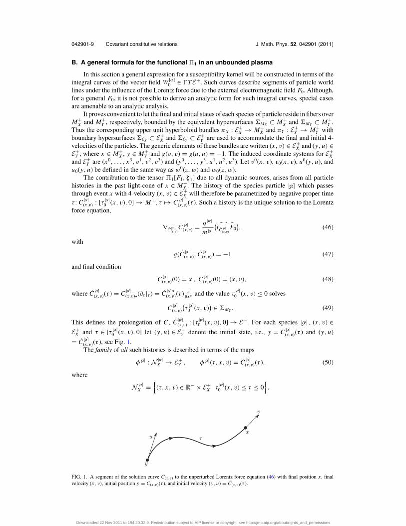
The contribution to the tensor �1[F1, ζ 1] due to all dynamic sources, arises from all particlehistories in the past light-cone of x ∈ M+

X . The history of the species particle �α� which passesthrough event x with 4-velocity (x, v) ∈ E+

X will therefore be parametrized by negative proper timeτ : C�α�

(x,v) : [τ �α�0 (x, v), 0] → M+, τ �→ C�α�

(x,v)(τ ). Such a history is the unique solution to the Lorentzforce equation,

∇C�α�(x,v)

C�α�(x,v) = q�α�

m�α�(

˜iC�α�(x,v)

F0), (46)

with

g(C�α�(x,v), C�α�

(x,v)) = −1 (47)

and final condition

C�α�(x,v)(0) = x , C�α�

(x,v)(0) = (x, v), (48)

where C�α�(x,v)(τ ) = C�α�

(x,v)�(∂τ |τ ) = C�α�a(x,v)(τ ) ∂

∂xa and the value τ �α�0 (x, v) ≤ 0 solves

C�α�(x,v)

(τ

�α�0 (x, v)

) ∈ �MY . (49)

This defines the prolongation of C , C�α�(x,v) : [τ �α�

0 (x, v), 0] → E+. For each species �α�, (x, v) ∈E+

X and τ ∈ [τ �α�0 (x, v), 0] let (y, u) ∈ E+

Y denote the initial state, i.e., y = C�α�(x,v)(τ ) and (y, u)

= C�α�(x,v)(τ ), see Fig. 1.The family of all such histories is described in terms of the maps

φ�α� : N �α�X → E+

Y , φ�α�(τ, x, v) = C�α�(x,v)(τ ), (50)

where

N �α�X =

{(τ, x, v) ∈ R− × E+

X

∣∣ τ �α�0 (x, v) ≤ τ ≤ 0

}.

y

ux

v

τ

FIG. 1. A segment of the solution curve C(x,v) to the unperturbed Lorentz force equation (46) with final position x , finalvelocity (x, v), initial position y = C(x,v)(τ ), and initial velocity (y, u) = C(x,v)(τ ).



The manifold N �α�X with boundary is naturally a fiber bundle over E+

X with projection � �α�X : N �α�

X

→ E+X , (τ, x, v) �→ �

�α�X (τ, x, v) = (x, v) and for any form α ∈ ��pNX it follows from (4) that

�∫�

�α�X

α = dx I ∧ dy J∫ 0

τ�α�0 (x,v)

α(1)(τ, x, v)dτ,

where α = α(1)(τ, x, v)dx I ∧ dy J ∧ dτ + α(2)(τ, x, v)dx I ∧ dy J .Let ��5

�EYE+

Y be the set of sections over �EY with values in �5E+Y , i.e., if α ∈ ��5

�EYE+

Y then

for each (y, u) ∈ �EY , α|(y,u) ∈ �5(y,u)E+

Y . Let the map ϕ�α� : ��5�EY

E+Y → ��5E+

X be given by

ϕ�α�(α)|(x,v) = φ�α��τ

�α�0 (x,v)

(α|τ

�α�0 (x,v)) ∈ �5

(x,v)E+X , (51)

where φ�α�τ : E+

X → E+, φ�α�τ (x, v) = φ(τ, x, v). For each species �α� let the initial data be given by

ζ�α�1 ∈ ��5

�EYE+

Y with iW �α�0ζ

�α�1 = 0.

In terms of these maps, it will now be shown that the general polarization functional �1 on M+X

is given by

�1[F1, ζ 1] =∑�α�

q�α� ��∫πX

�∫�

�α�X

dτ ∧ φ�α��(iW �α�1 (F1)θ

�α�0 ) + �d

(�1[F1]

)+

∑�α�


ϕ�α�(ζ �α�1 ) + �d

(Z1[ζ 1]

),

(52)

where�1 and Z1 are arbitrary linear functionals of F1 and ζ 1, respectively. The excitation�1[F1, ζ 1],in (52), is the general solution to (44) where the source θ1 satisfies (38) and (39). The first two termson the right hand side of (52) are linear functionals of F1 whereas the last term is a linear functionalof the initial data ζ 1. Clearly �d

(�1[F1]

)and �d

(Z1[ζ 1]

)are in the kernel of d�, the homogeneous

differential operator associated with (44).The proof that (52) solves (44) requires the following lemma which is proved in the Appendix.

Lemma 1: Let N be a manifold with a boundary �N ⊂ N and let V ∈ �T N be a nonvanishingvector field on N such that every integral curve of V intersects �N precisely once. For each σ ∈ Nlet the integral curve of V terminating at σ be given by γσ : [τ0(σ ), 0] → N, where γσ (0) = σ andγσ (τ0(σ )) ∈ �N . The set N = {

(σ, τ ) ⊂ R− × N∣∣ τmin(σ ) ≤ τ ≤ 0

}is a fibered manifold over N

with projection �N : N → N, (τ, σ ) �→ �N (τ, σ ) = σ . The family of integral curves of V can bedescribed by the map φN : N → N, φN (τ, σ ) = γσ (τ ). Let ζ ∈ ��

p�N

N such that iV ζ = 0, i.e.,ζ is a p-form on �N with values in �p N . Let ϕN : ��p

�NN → ��p N be given by ϕN (ζ )|σ =

φ�N τ0(σ )(ζ |τ0(σ )) ∈ �p�N

N .If β ∈ ��p N is a p-form on N with compact support such that iVβ = 0 and ξ ∈ ��p N has

the form

ξ = �∫�N

φ�N (β) ∧ dτ + ϕN (ζ ) (53)

then

iV dξ = β, (54)

ξ |�N = ζ .This lemma is applied with N = E+

X , �N = ��α�X , V = W �α�

0 , τ0 = τ�α�0 , φN = φ�α�, ϕN = ϕ�α�,

ζ = ζ�α�1 , and

β = −iW �α�1 (F1)θ

�α�0 . (55)

Thus ξ in (53) becomes the 5-form ξ�α�1 ∈ ��5E+

X ,

ξ�α�1 = −�

∫�

�α�X

φ�α��(iW �α�1 (F1)θ

�α�0

) ∧ dτ + ϕ�α�(ζ �α�1 ) = �

∫�

�α�X

dτ ∧ φ�α��(iW �α�1 (F1)θ

�α�0

) + ϕ�α�(ζ �α�1 ),

(56)



since deg(φ�α��(iW �α�

1 (F1)θ�α�0 )

) = 5. In order to satisfy (38) let

θ�α�1 = dξ �α�

1 . (57)

Furthermore, from (54) and (55)

iW �α�0θ

�α�1 = iW �α�

0dξ �α�

1 = −iW �α�1 (F1)θ

�α�0

so (39) is satisfied. In terms of ξ �α�1 (52) can be written

�1[F1, ζ 1]|x =∑�α�


ξ�α�1 + �d

(�1[F1]

)|x + �d(Z1[ζ 1]

).

Then from (5)

d � �1[F1, ζ 1] = d � �( ∑

�α�q�α��

∫πX

ξ�α�1

)

= −∑�α�

q�α�d�∫πX

ξ�α�1 = −

∑�α�

q�α��∫πX

dξ �α�1

= −∑�α�

q�α��∫πX

θ�α�1 .

Thus the Maxwell equation (44) is also satisfied. That (52) is the general solution to (44) follows fromthe fact that the difference between any two solutions of (44) satisfies the homogeneous differentialequation associated with (44).

Thus we have succeeded in eliminating θ �α�1 from the perturbation system (38)–(41), thereby

reducing the system to d F1 = 0 and

ε0d � F1 + 12

∑�α�

q�α�d�∫πX

�∫�

�α�X

dτ ∧ φ�α��(iW �α�1 (F1)θ

�α�0 ) +

∑�α�

q�α�d�∫πX

ϕ�α�(ζ �α�1 ) = 0 (58)

in terms of (θ0, F0), for the perturbation F1. The perturbation θ1 is then given by (57) and (56).

C. The susceptibility kernel for an unbounded collisionless plasma

Equating (52) and (45) with the initial data,

Z1[ζ 1] =∑�α�


ϕ�α�(ζ �α�1 ) + �d

(Z1[ζ 1]

), (59)

yields

�∫

pX

χ ∧ p�Y (F1) =∑�α�


�∫�

�α�X

dτ ∧ φ�α��(iW �α�1 (F1)θ

�α�0 ) + �d

(�1[F1]

)(60)

Away from the initial hypersurface boundary ∂(M+X × M+

Y ) = �MX × M+Y ∪ M+

X ×�MY , using (5)and (A2) one has

�∫

pX

�X dX ξ ∧ p�Y (F1) = �∫

pX

�X d ξ ∧ p�Y (F1) = �d�∫

pX

ξ ∧ p�Y (F1) = �d(�1[F1]

),

where �1[F1] is a linear functional of F1. The gauge freedom χ → �X dX ξ given in (10) is equivalentto the addition of the term �d

(�1[F1]

)in (52).

If F1 is restricted to have support in a certain domain one may find χ such that

�∫

pX

χ ∧ p�Y (F1) =∑�α�


�∫�

�α�X

dτ ∧ φ�α��(iW �α�1 (F1)θ

�α�0 ). (61)



To find such a susceptibility kernel requires the following maps.For (y, u) ∈ E+

Y , let C�α�(y,u) : R+ → M+ and C�α�

(y,u) : [0, τ �α�1 (y, u)

) → E+ be the unique solutionsto the unperturbed Lorentz force equation (46) and (47) with initial conditions

C�α�(y,u)(0) = y C�α�

(y,u)(0) = (y, u), (62)

where τ �α�1 (y, u) ∈ R+ ∪ {∞} is the supremum of the values of τ such that C�α�

(y,u)(τ ) ∈ M . Let

��α� : N �α�Y → M+

X × M+Y ,

��α�(τ, y, u) = (C�α�

(y,u)(τ ), y), (63)

where

N �α�Y =

{(τ, y, u) ∈ R+ × E+

X

∣∣ 0 ≤ τ < τ�α�1 (y, u)

}.

This map gives the final and initial positions of a solution to the unperturbed Lorentz force equationin terms of the initial position, velocity, and proper time parameter τ ∈ [0, τ �α�

1 (y, u)).

Observe that��α� is never surjective, since if��α�(τ, y, u) = (x, y) then x ∈ J+(y). Also��α� isnever injective since��α�(0, y, u) = (y, y) for all (y, u) ∈ E+

Y . Thus��α� does not possess an inverseand one must work locally on M+

X × M+Y in order to establish the diffeomorphism ��α� : D → D′,

��α� = (��α�|D′

)−1, (64)

i.e.,

��α�(C(y,u)(τ ), y) = (τ, y, u)

with D ⊂ M+X × M+

Y and D′ ⊂ N �α�Y given by

D ={

(x, y)

∣∣∣∣ There exists a unique u∈Ey and τ∈R+ such that C�α�(y,u)(τ ) = x for all �α�

}, (65)

D′ ={

(τ, y, u)∣∣∣��α�(τ, y, u) ∈ D for all �α�

}.

This map ��α� encodes the solution to the 2-point problem, namely given an initial event y ∈ MY

and final event x ∈ MX find the unique worldline to the unperturbed Lorentz force equation whichpasses though these two points. This worldline is specified by its initial velocity (y, u) ∈ E+

X and itsproper time τ . The statement that ��α� does not have an inverse is equivalent to the statement thatin general there may not be a unique solution to the two point problem on an arbitrary domain. Thedomain D is the set of all pairs (x, y) such that there is a unique worldline.

Set

χ =∑�α�χ �α�, (66)

where

χ �α�|(x,y) = 12

q�α� 2

m�α� �X dycd ∧ i (y)abcd�

�α��(

dτ ∧��α��Y

(gνaubi (u)

ν θ�α�0

))∣∣∣(x,y)

(67)

for points (x, y) ∈ D. In the Appendix (Lemma 6) it is shown that given x ∈ M+X (61) and F1 with

support in

Dx = D ∩ p−1X {x} = {y ∈ MY |(x, y) ∈ D} (68)

then (61) holds at x . Furthermore, although (dYχ )|(x,y) is unique, χ has the gauge freedom given by(9).

One may write (67) implicitly as

χ �α� ∧ p�Yγ = −q�α� �X S��α��(

dτ ∧��α��Y (i

W�α�1 (γ )

θ�α�0 )

)(69)



for all γ ∈ ��2 M+Y where S : �6

(x,y)(M+X × M+

Y ) → �6(x,y)(M+

X × M+Y ),

S(α) = i (y)0123α ∧ dy0123. (70)

The tensor projector S has the simplest representation in the coordinate basis employed here sincei (y)a dyb = δb

a .From (64) for a chosen species �α� one must consider τ and u to be functions of (x, y) as well as

the species label �α�. Thus let��α� be given by the functions τ = τ (x, y) and uμ = uμ(x, y), wherewe have dropped the species label, i.e., τ (x, y) and uμ(x, y) solve the implicit equation

C�α�(y,u(x,y))

(τ (x, y)

) = x, (71)

where u0(x, y) is the solution to ua(x, y)ub(x, y)gab(y) = −1 and u0(x, y) = ga0(y)ua(x, y). Letf �α�0 = f �α�

0 (y, u) represent the unperturbed probability function on E+Y . The contribution to the

susceptibility kernel from species �α� is given in local coordinates by (Lemma 7 in the Appendix.)

χ �α�|(x,y) = − f �α�0

q�α�2

m�α�| det g|3/2

4u0gμcubεdejkεcbihεμνσ×(

ua

2

∂τ

∂ya

∂uν

∂xd

∂uσ

∂xe− ua

2

∂τ

∂xd

∂uν

∂ya

∂uσ

∂xe+ ua

2

∂τ

∂xd

∂uν

∂xe

∂uσ

∂ya

+ ( − �ν p f u pu f + q�α�

m�α� F0p f gνpu f) ∂τ∂xd

∂uσ

∂xe

)dx jk ∧ dyih,

(72)

where g, F0, and �ν e f are all evaluated at y ∈ M+Y and each τ and u belongs to the species �α�. This

is a key result of our article.

D. A spacetime inhomogeneous microscopically neutral plasma

In a Vlasov model, a plasma or gas is deemed microscopically neutral if in its unperturbedstate F0 = 0. Let M be Minkowski spacetime with global Lorentzian coordinates so that �νab = 0.Assume that f �α�

0 solves the zeroth order Maxwell–Vlasov system (35) with θ �α�0 = i

W�α�0

( f �α�0 �) and

F0 = 0. In this scenario one can calculate χ explicitly.Since Minkowski spacetime is flat and F0 = 0 the integral curves C(x,v) in global Lorentzian

coordinates are the straight lines

τ =√

−g(x − y, x − y) u = (x − y)

τ. (73)

Differentiating with respect to xa and ya gives

∂τ

∂xa= −ua ,

∂τ

∂ya= ua ,

∂ua

∂xb= (δa

b + uaub)

τ,

∂ua

∂yb= − (δa

b + uaub)

τ. (74)

If follows from (72) that

χ �α�|(x,y) = q�α� f�α�0 (y,u)

4u0τ 2 gμcubεcbih(2dx0μ + εdσ jkεμνσuνuddx jk

) ∧ dyih, (75)

where τ (x, y) and u(x, y) are given by (73).It is often useful to explore the response of an inhomogeneous plasma due to a monochromatic

electromagnetic plane wave with constant amplitude E ,

F1 = Ee−iωx0+ikx1dx01 . (76)

Setting the initial hypersurface as �EY = {y0 = y0

0

}, the general initial 5-form ζ

�α�1 ∈ ��5

�EYE+

Y

satisfying iW0ζ�α�1 = 0 is given in terms of its components by

ζ�α�1 |(0,yμ,uν ) = (

u0dy1 − u1dy0) ∧ (

ζ�α�1,1dy2 ∧ du123 + ζ

�α�1,2dy3 ∧ du123

) + ζ�α�1,3dy23 ∧ du123

+(u0dy123 − u1dy023

)(ζ

�α�1,4du12 + ζ

�α�1,5du13 + ζ

�α�1,6du23

),

(77)



where ζ �α�1,A = ζ

�α�1,A(yμ, uν) for A = 1, . . . 6. For the integral curves (73) and the initial hypersurface

�EY = {y0 = y0

0

}one has τ0(x, v) = (y0

0 − x0)/v0 and the map ϕ is given by (51) with φ�τ (ya) =xa + τ ya and φ�τ (ua) = va . From (45) with χ given by (75) and Z1[ζ 1] given by (59) one has

�1[F1, ζ 1] =

−∑�α�

q�α� 2

m�α� Ee−iωx0+ikx1

{dx01

∫dv123T �α� (v0)2 − (v1)2

v0+ dx12

∫dv123T �α�v2

−dx02∫

dv123T �α� v2v1

v0+ dx13

∫dv123T �α�v3 + dx03

∫dv123T �α� v

3v1

v0

}

+∑�α�

q�α�{

dx02∫

dv123(ζ

�α�1,4

v1(x0 − y00 )

v0− ζ

�α�1,1v

1)

+dx03∫

dv123(ζ

�α�1,5

v1(x0 − y00 )

v0− ζ

�α�1,2v

1)

+dx12∫

dv123(v0ζ

�α�1,1 − ζ

�α�1,4(x0 − y0

0 ))

+ dx13∫

dv123(v0ζ

�α�1,2 − ζ

�α�1,5(x0 − y0

0 ))

+dx23∫

dv123

(ζ

�α�1,3 + ζ

�α�1,4

v1v3(x0 − y00 )

(v0)2− ζ

�α�1,5

v1v2(x0 − y00 )

(v0)2+ ζ

�α�1,6(x0 − y0

0 )(v1

v0− 1

))}

+ � d(�1[F1]

) + �d(Z1[ζ 1]

), (78)

where∫

dv123 denotes the triple integral operator� ∞

−∞ dv123, v0 = √1 + vμvμ,

T �α� = T �α�(x, v) =∫ 0

(y00 −x0)/v0

eiτ (−ωv0+kv1) f �α�0 (x + τv, v)τdτ, (79)

and ζ �α�1,A = ζ

�α�1,A(xμ, vμ) = ζ

�α�1,A

(xμ − x0vμ/v0, vν

)in (78). This response is not in general plane

fronted.For the particular case of a plane fronted plasma distribution,

f �α�0 (x, v) = h�α�

0 (x0, x1, v1)δ(v2)δ(v3), (80)

with initial data,

ζ�α�1 = 0,

(78) becomes the plane fronted 2-form,

�1[F1, ζ ]|x

= −dx01∑�α�

q�α� 2

m�α� Ee−iωx0+ikx1∫ ∞

−∞dv1

∫ 0

(y00 −x0)/v0

dτ eiτ (−ωv0+kv1)h�α�0 (x0 + τv0, x1 + τv1, v1)

τ

v0

+ � d(�1[F1]

), (81)

describing the response of a spacetime inhomogeneous unbounded plasma to (76).

E. Spacetime homogeneous unbounded plasmas

The previous discussion simplifies considerably if the unperturbed plasmas is homogeneous inspace and time. In Minkowski spacetime M , an unbounded unperturbed plasma is deemed spacetimehomogeneous if A�z F0 = F0 and A�zθ

�α�0 = θ

�α�0 for all z ∈ M , where the translation map Az : M → M ,

Az(x) = x + z induces the map Az : E → E , Az = Az�. Such spacetime homogeneity implies that



in all inertial frames the medium is stationary and spatially homogeneous in all directions. Sucha spacetime homogeneous plasma will give rise to a spacetime homogeneous electromagneticconstitutive relation. In addition to the components (F0)ab with respect to an inertial frame beingconstant, the functions f �α�(x, v) are independent of event position x and can therefore be writtenf �α�(v).

In this scenario the Fourier transform (17) of the susceptibility kernel (18) for each species, isthen given by

χ �α�ab

e f (k)dxab

= 12 q�α�dxgh

∫ 0

−∞dτ

∫dv123 f �α�

0 (v)e−ik·L�α�v vg

v0

(gνeu f −gν f ue

)(L�α�

νh(τ ) − uν

u0L�α�

0h(τ )

),

(82)

where F0 is the 4 × 4 real matrix with components (F0)ab = ηac(F0)cb generating the matrices

D�α�ab(τ ) = exp

(τ

q�α�m�α� F0

)a

b, D�α�

ba(τ ) = gbc D�α�c

d (τ )gda ,

L�α�ab(τ ) =

∫ τ

0D�α�a

b(τ ′) dτ ′, L�α�b

a(τ ) = gbc L�α�cd (τ )gda ,

(83)

k · L�α�v = ka L�α�ab(τ )vb,

ua(τ, v1, v2, v3) = D�α�ab(τ )vb. (84)

The susceptibility kernel (82) can be shown to agree with the results of O’Sullivan and Derfler.12

Furthermore, for a microscopically neutral spacetime homogeneous plasma with F0 = 0,G1 = 0, and f �α�

0 (v) = h�α�0 (v1)δ(v2)δ(v3) it follows from (81) and (43) that for Im(ω) > 0,

1 =∑�α�

q�α� 2

m�α�ε0

∫ ∞

−∞

h�α�0 (v1) dv1

v0(−ωv0 + kv1)2. (85)

The relativistic Landau damped dispersion relation for plane fronted Langmuir modes in an unper-turbed spacetime homogeneous plasma arises by analytic continuation of the integral (85) to thelower-half complex ω plane.

F. Langmuir modes for an inhomogeneous unbounded plasma in Minkowski spacetime

If the plasma is microscopically neutral but spacetime inhomogeneous in its unperturbed state theLandau dispersion relation corresponding to (85) becomes more involved. We define the generalizedLangmuir sector to contain perturbations described by (81) but with the external polarization specifiedby �1[F1] set to zero. Since ζ �α�

1 = 0, �1[F1, 0] will be denoted �1[F1]. Thus (43) with G1 = 0becomes

ε0 F1 = −�1[F1]. (86)

Consider the case where planar inhomogeneities in a plasma composed of electrons and ions arisefrom the unperturbed spacetime inhomogeneous solution to the Maxwell–Vlasov system Eqs. (35)and (36) with F0 = 0 and

f �el�0 (x0, x1, x2, x3, v1, v2, v3) = f �ion�

0 (x0, x1, x2, x3, v1, v2, v3)

= h(

x1 − v1x0

v0, v1

)δ(v2)δ(v3),

(87)

where q�el� = −q�ion�.



For example, one might consider

h(x1, v1) = n�ion�(x1)A�ion�(x1) exp(

− m�ion�v0

kB T �ion�(x1)

),

where A�ion�(x1) normalizes (87). Then f �ion� initially at x0 = 0 represents a distribution ofions where, at each spatial point x1, the velocities belong to the one-dimensional Maxwell–Juttner distribution. In such a distribution the temperature T �ion�(x1) and the number den-sity of ions n�ion�(x1) depend on position. It follows from (87) that f �el� also initially repre-sents a position dependent Maxwell–Juttner distribution, where n�el�(x1) = n�ion�(x1) and T �el�(x1)= T �ion�(x1)m�el�/m�ion�. After the initial moment, the ions and electrons drift according to (87) andvelocities do not remain in the Maxwell–Juttner distributions. Alternatively (87) might describe aplasma composed of particles and antiparticles.

In the theory of a spacetime homogeneous plasma ω and k satisfy the transcendental dispersionrelation (85). This relation contains an integral that is potentially singular. The Landau prescriptioncircumvents this singularity by complexifyingω and defining an analytic continuation for the integralin the complex ω plane.

Setting h�α�0 (x0, x1, v1) = h

(x1 − v1x0/v0, v1

)in (80) yields (87) and (81) becomes

�1[F1]|x

=−dx01q�el� 2( 1

m�ion� + 1

m�el�)

Ee−iωx0+ikx1∫ ∞

−∞dv1h

(x1−v1x0

v0,v1

)∫ 0

(y00 −x0)/v0

dτ eiτ (−ωv0+kv1) τ

v0.

(88)

To compare with the results (85) given for the homogeneous case, consider the limit y00 → −∞

with Im(ω) > 0. Furthermore, for the nonevanescent modes considered here Im(k) = 0. Thus (88)becomes

�1[F1]|x = −dx01ε0Q20 Ee−iωx0+ikx1

∫ ∞

−∞dv1 h(x1 − v1x0/v0, v1)

v0(−ωv0 + kv1)2, (89)

where

Q20 = q�el� 2

ε0m�ion� + q�el� 2

ε0m�el� .

In a spacetime inhomogeneous plasma there is no time-harmonic solution or associated transcen-dental dispersion relation between ω and k. We therefore propose solving (86) with a longitudinalfield F1 represented as the packet

F1(x0, x1) = dx01∫ ∞

−∞dω

∫ ∞

−∞dk E(ω, k)e−iωx0+i kx1

. (90)

Substituting (89) and (90) into (86) yields∫ ∞

−∞dω

∫ ∞


= Q20

∫ ∞

−∞dω

∫ ∞


∫ ∞

−∞dv1 h(x1 − v1x0/v0, v1)

v0(ωv0 + kv1)2.

Performing the inverse Fourier transform gives

4π2 E(ω, k)

= Q20

∫ ∞

−∞dx0

∫ ∞

−∞dx1

∫ ∞

−∞dω

∫ ∞

−∞dk E(ω, k)ei(−(ω−ω)x0+(k−k)x1)

∫ ∞

−∞dv1 h(x1 − v1x0/v0, v1)

v0(ωv0 + kv1)2.



Since ∫ ∞

−∞dx0

∫ ∞

−∞dx1ei(−(ω−ω)x0+(k−k)x1)h(x1 − v1x0/v0, v1)

= 2π h(k − k, v1)δ(ω − ω + v1(k − k)/v0),

where

h(k, v1) =∫ ∞

−∞e−iksh(s, v1)ds,

one has

E(ω, k) = Q20

2π

∫ ∞

−∞dω

∫ ∞

−∞dk

∫ ∞

−∞dv1 E(ω, k)

v0(ωv0 + kv1)2h(k − k, v1)δ

(ω − ω + v1(k − k)/v0

).

(91)

Since we restrict to nonevanescent modes k and k are real. For E(ω, k) to be nonzero one requiresthe argument of the δ-function to be zero. Since v1 is real and therefore v1(k − k)/v0 is real itfollows that although Im(ω) > 0 and Im(ω) > 0 the difference ω − ω is real. Furthermore, fromω − ω + v1(k − k)/v0 = 0 it follows that |ω − ω| < |k − k|. Thus (91) becomes

E(ω, k) = Q20

2π

∫ ∞

−∞dk I (ω, k, k), (92)

where

I (ω, k, k) =∫

S(ω,k,k)dω E(ω, k)

(k − k)

(ωk − kω)2h

(k − k,

k − k√(k − k)2 − (ω − ω)2

)(93)

and the contour of integration for ω in (93) is the straight line S(ω, k, k) where Im(ω) = Im(ω) > 0and −|k − k| < Re(ω − ω) < |k − k|. Since (ω − ω)2 < (k − k)2 the arguments of h in (93) arealways real and nonsingular on S(ω, k, k).

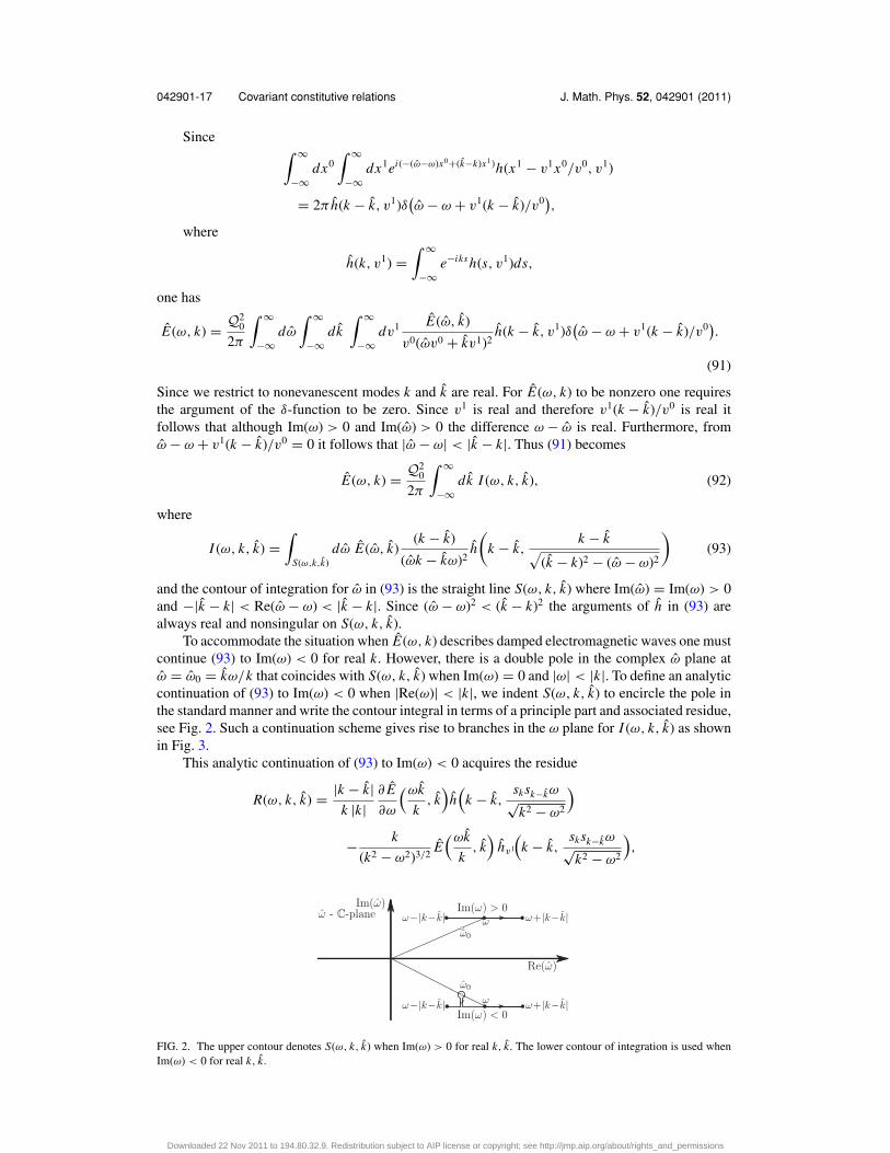
To accommodate the situation when E(ω, k) describes damped electromagnetic waves one mustcontinue (93) to Im(ω) < 0 for real k. However, there is a double pole in the complex ω plane atω = ω0 = kω/k that coincides with S(ω, k, k) when Im(ω) = 0 and |ω| < |k|. To define an analyticcontinuation of (93) to Im(ω) < 0 when |Re(ω)| < |k|, we indent S(ω, k, k) to encircle the pole inthe standard manner and write the contour integral in terms of a principle part and associated residue,see Fig. 2. Such a continuation scheme gives rise to branches in the ω plane for I (ω, k, k) as shownin Fig. 3.

This analytic continuation of (93) to Im(ω) < 0 acquires the residue

R(ω, k, k) = |k − k|k |k|

∂ E

∂ω

(ωk

k, k

)h(

k − k,sksk−kω√k2 − ω2

)

− k

(k2 − ω2)3/2E

(ωk

k, k

)hv1

(k − k,

sksk−kω√k2 − ω2

),

ω - C-planeIm(ω)

Re(ω)

Im(ω) > 0

Im(ω) < 0

ω

ω

ω0

ω0

ω+|k−k|ω−|k−k|

ω+|k−k|ω−|k−k|

FIG. 2. The upper contour denotes S(ω, k, k) when Im(ω) > 0 for real k, k. The lower contour of integration is used whenIm(ω) < 0 for real k, k.



ω - C-planeIm(ω)

Re(ω)

|k|− |k|

bran

chcu

t

bran

chcu

t

√k2 − ω2 > 0

FIG. 3. Branch cuts in ω for I (ω, k, k).

where hv1 (k, v1) = ∂ h∂v1 (k, v1), sk = k/|k|, and sk−k = (k − k)/|k − k|. In the case when Im(ω) = 0,

the principle value of (93) is taken together with residue 12 R(ω, k, k). Equation (92) then gives

E(ω, k) = k

2π

∫ ∞

−∞I (ω, k, k) dk if Im(ω) > 0 or |Re(ω)| > |k|,

E(ω, k) = k

2π

∫ ∞

−∞I (ω, k, k) dk − ik

∫ ∞

−∞R(ω, k, k) dk

if Im(ω) < 0 and |Re(ω)| ≤ |k|,

E(ω, k) = k

2π

∫ ∞

−∞P I (ω, k, k) dk − ik

2

∫ ∞

−∞R(ω, k, k) dk

if Im(ω) = 0 and |Re(ω)| < |k|,(94)

where P I (ω, k, k) in (94) refers to the principle part of (93) when Im(ω) = 0 and |Re(ω)| < |k| andhence the pole at ω0 lies on the contour S(ω, k, k). Thus in each domain above, the perturbationE(ω, k) must be determined by solving a nonstandard integral equation.

IV. CONCLUSIONS

In this article a classical covariant description of electromagnetic interactions in continuousmatter in an arbitrary background gravitational field has been formulated in terms of a polarization2-form that enters into the macroscopic Maxwell equations. Linear dispersive constitutive rela-tions arise when this 2-form is expressed as an affine functional of the Maxwell 2-form with theaid of a 2-point susceptibility kernel. We have explored the constraints on this kernel imposedby causality requirements, spacetime Killing symmetries and local gauge freedoms. The formal-ism has been applied to an analysis of constitutive models for waves in collisionless plasmas. Inparticular a formula for the linear susceptibility of a fully ionized inhomogeneous unbounded non-stationary collisionless plasma to a perturbation in the presence of gravity has been given in termsof maps describing the dynamics of the plasma. This formula has been elucidated by referenceto both homogeneous and inhomogeneous perturbations in Minkowski spacetime. In the formercase one recovers the standard Landau dispersion relation when perturbing Langmuir modes. Inthe latter case we have described a generalized damping mechanism for such modes that mayarise when the unperturbed state is both inhomogeneous and nonstationary. Such a mechanismarises from the analytic continuation of an integral equation that replaces the Landau dispersionrelation.

It is concluded that the use of a covariant 2-point affine susceptibility kernel in describingthe electromagnetic response of dispersive media offers a modeling tool that naturally generalizesthe use of permittivity and permeability tensors used to model electromagnetic interactions innonrelativistic media. The formulation in terms of an arbitrary background spacetime metric offers



potential applications in a number of astrophysical contexts involving electromagnetic fields ininhomogeneous or nonstationary plasmas.

ACKNOWLEDGMENTS

The authors are grateful to support from Engineering and Physical Sciences Research Consul(U.K.) (EPSRC)(EP/E001831/1) and the Cockcroft Institute (STFC ST/G008248/1).

APPENDIX: PROOFS OF RESULTS USED USED IN THE TEXT

Lemma 2: Local representation of �∫πNα in (4) from the implicit definition in Eq. (3).

Proof: On a fibered manifold N of dimension n + r with projection πN : N → N overa manifold N of dimension n. Thus at each point σ ∈ N one has the fiber Nσ = π−1

N {σ }= {

(σ ′, ς ) ∈ N∣∣πN (σ ′, ς ) = σ

}so dim(Nσ ) = r is the fiber dimension. Let (σ 1, . . . , σ n) and

(σ 1, . . . , σ n, ς1 . . . ς r ) be local coordinates for patches on N and N , respectively.Consider first the case when α ∈ ��p+rN consists of a single component αI (σ, ς )dσ I ∧

dς1...r with no sum on I . Hence explicit summation will be used in this particular proof.Set I = {1, . . . , n}\I so that dσ I ∧ dσ I = ±dσ 1...n and let β = ∑

J βJ (σ )dσ J then β ∧ dσ I

= ±β IαI dσ 1...n so that

∑J

∫(σ,ς)∈N

π�N (βJ (σ )dσ J ) ∧ αI (σ, ς )dσ I ∧ dς1...r

=∑

J

∫(σ,ς)∈N

βJ (σ )dσ J ∧ αI (σ, ς )dσ I ∧ dς1...r

=∑

J

∫(σ,ς)∈N

βJ (σ )dσ J ∧ dσ I ∧ αI (σ, ς )dς1...r

=∫

(σ,ς)∈Nβ I (σ )dσ I ∧ dσ I ∧ αI (σ, ς )dς1...r

=∫σ∈N

β I (σ )dσ I ∧ dσ I∫Nσ

αI (σ, ς )dς1...r

=∑

J

∫σ∈N

βJ (σ )dσ J ∧ dσ I∫Nσ

αI (σ, ς )dς1...r

=∫σ∈N

β ∧ dσ I∫Nσ

αI (σ, ς )dς1...r .

Thus by linearity ∫Nπ�N (β) ∧ α =

∑I

∫σ∈N

β ∧ dσ I∫Nσ

αI (σ, ς )dς1...r , (A1)

where α = ∑I αI (σ, ς )dσ I ∧ dς1...r . If (4) holds then for α = ∑

I αI (σ, ς )dσ I ∧ dς1...r ,∫Nβ ∧ �

∫πN

α =∑

I

∫Nβ ∧ dσ I

∫ς∈Nσ

i (σ )I α|(σ,ς) =

∑I

∫Nβ ∧ dσ I

∫ς∈Nσ

αI dς1...r

=∫Nπ�N (β) ∧ α.



Hence (3). Conversely if (3) holds for α = ∑I αI (σ, ς )dσ I ∧ dς1...r then from (A1)∫

Nβ ∧ �

∫πN

α =∫Nπ�N (β) ∧ α =

∑I

∫Nβ ∧ dσ I

∫ς∈Nσ

i (σ )I α|(σ,ς).

Since this is true for all β then (4) holds.If α does not contain the factor ς1...r , i.e., α = αI K (σ, ς )dσ I ∧ dς K , where K �= {1, . . . , r}

then the right hand side of (3) becomes∫Nπ�N (β) ∧ α =

∑J

∫NβJαI K (σ, ς )dσ J ∧ dσ I ∧ dς K = 0

and the right hand side of (4) becomes

∑I

dσ I∫ς∈Nσ

αI K (σ, ς )dς K = 0.

Thus by linearity (3) and (4) are equivalent for all α. �Lemma 3: Verification of Eq. (5)(

d�∫

πN

α

)∣∣∣∣σ

=(

�∫

πN

dα

)∣∣∣∣σ

.

Proof Let deg(α) = p + r , deg(β) = n − p − 1 and ∂N and ∂N be the boundaries of N andN . Since σ /∈ ∂N one may choose β to have support away from ∂N thus∫

∂Nβ ∧

(�∫

πN

α)

= 0

and since α has support away from ∂N then∫∂Nπ�Nβ ∧ α = 0.

It follows that∫Nβ ∧

(�∫

πN

dα)

=∫Nπ�N (β) ∧ dα

= (−1)n−p−1∫N

d(π�N (β) ∧ α

) + (−1)n−p∫N

dπ�N (β) ∧ α

= (−1)n−p−1∫∂Nπ�N (β) ∧ α + (−1)n−p

∫Nπ�N (dβ) ∧ α

= (−1)n−p∫

Ndβ ∧

(�∫

πN

α)

= (−1)n−p∫

Nd(β ∧

(�∫

πN

α))

+∫

Nβ ∧ d

(�∫

πN

α)

= (−1)n−p∫∂Nβ ∧

(�∫

πN

α)

+∫

Nβ ∧ d

(�∫

πN

α)

=∫

Nβ ∧ d

(�∫

πN

α). �



Lemma 4: Proof of

�∫

pX

�Xα = ��∫

pX

α. (A2)

Proof: The only nontrivial α ∈ ��(MX × MY ) in (A2) can be written α = αI dx I ∧ dy0123.Then

�∫

pX

�X(αI dx I ∧ dy0123

) = �∫

pX

αI (�dx I ) ∧ dy0123 = �dx I

∫MX

αI dy0123 = ��∫

pX

αI dx I ∧ dy0123.

�Lemma 5: � is causal on M+

X if and only if

• Z is causal on MX+,

• (dYχ )|(x,y) = 0 for all (x, y) ∈ M+X × M+

Y such that y /∈ J−(x), and

• ι��MY(χ )

∣∣(x,y) = 0 for all (x, y) ∈ M+

X ×�MY such that y /∈ J−(x), where

ι�MY: M+

X ×�MY ↪→ M+X × M+

Y is the natural embedding.

(A3)

Proof: If ι�MY: �MY ↪→ M+

Y is the natural embedding then i (x)ab ι

��MY

χ |(x,y) = ι��MYi (x)ab χ |(x,y) and∫

y∈M+Y

i (x)ab

(χ | ∧ p�Y (d A|y)

)=

∫y∈M+

Y

i (x)ab

(χ ∧ dY (p�Y A)

)|(x,y)

=∫

y∈M+Y

i (x)ab dY

(χ ∧ p�Y A|y

)∣∣(x,y) −

∫y∈M+

Y

i (x)ab

(dYχ ∧ p�Y A|y

)∣∣(x,y)

=∫

y∈M+Y

dY(i (x)ab χ ∧ p�Y A|y

)∣∣(x,y) −

∫y∈M+

Y

i (x)ab

(dYχ ∧ p�Y A|y

)∣∣(x,y)

=∫

y∈�MY

ι��MYi (x)ab

(χ ∧ p�Y A|y

)∣∣(x,y) −

∫y∈M+

Y

i (x)ab

(dYχ ∧ p�Y A|y

)∣∣(x,y)

=∫

y∈�MY \J−(x)i (x)ab ι

��MY

(χ ∧ p�Y A|y

)∣∣(x,y) +

∫y∈�MY ∩J−(x)

i (x)ab ι

��MY

(χ ∧ p�Y A|y

)∣∣(x,y)

−∫

y∈M+Y \J−(x)

i (x)ab

(dYχ ∧ p�Y A|y

)∣∣(x,y) −

∫y∈M+

Y ∩J−(x)i (x)ab

(dYχ ∧ p�Y A|y

)∣∣(x,y).

(A4)

First one argues that (A3) implies that� is causal on M+X . Given x ∈ M+

X and F1, F2 ∈ ��2 M+Y

such that F1|y = F2|y = 0 for y ∈ J−(y), set F = F1 − F2 so that F = 0 on J−(x). Since M+Y

is topologically trivial F is exact, F = d A, and hence d A = 0 on J−(x). Then since J−(x) istopologically trivial there exists f ∈ ��0 M+

Y such that A = d f on J−(x). Thus one can choose agauge A = A − d f so that A = 0 on J−(x). Given ζ such that ζ |y = 0 for y ∈ J−(x) ∩�MY thenZ [ζ ]|x = 0 since Z is causal. Thus from (A4)

�[F, ζ ]ab(x) =∫

y∈M+Y

i (x)ab

(χ | ∧ p�Y (d A|y)

)

=∫


��MY

(χ ∧ p�Y A|y

)∣∣(x,y) +

∫y∈�MY ∩J−(x)

i (x)ab ι

��MY

(χ ∧ p�Y A|y

)∣∣(x,y)

−∫

y∈M+Y \J−(x)

i (x)ab

(dYχ ∧ p�Y A|y

)∣∣(x,y) −

∫y∈M+

Y ∩J−(x)i (x)ab

(dYχ ∧ p�Y A|y

)∣∣(x,y) = 0,

since ι��MYχ |(x,y) = 0 for y ∈ �MY \J−(x), A|y = 0 for y ∈ J−(x), and dYχ = 0 for y ∈ M+

Y \J−(x).



Conversely if� is causal on M+X then setting F = 0 in (6) shows that Z must be causal on M+

X .Then setting ζ = 0 then for all A such that A = 0 on J−(x) (A4) yields

0 = �[F, ζ ]ab(x)

=∫


��MY

(χ(x,y) ∧ p�Y A|y

)∣∣(x,y) −

∫y∈M+

Y \J−(x)i (x)ab

(dYχ(x,y) ∧ p�Y A|y

)∣∣(x,y). (A5)

The four-dimensional domain M+Y \J−(x) denotes points outside the backward light-cone of x , while

the three-dimensional domain�MY \J−(x) denotes the points on�MY that are not causally connectedto x . Choosing such an A to have support about a small neighborhood of y ∈ M+

Y \J−(x)\�MY resultsin the first term of (A5) being zero and thus (dYχ )|(x,y) = 0. Likewise setting A to have supportabout a small neighborhood of y ∈ �MY \J−(x) implies ι��MY

(χ )|(x,y) = 0. �One can now prove Lemma 1 in Sec. III B.

Proof of Lemma 1: Given σ ∈ N , with V nonvanishing there exists a coordinate system(σ 1, . . . , σ n) on N adapted to V so that V = ∂

∂σ 1 and the image of the curve γσ : [τ0(σ ), 0] → Nis contained in the coordinate patch. Write β = βI dσ I then since iVβ = 0 the sum is overI ∈ {2, . . . , n}. With σ 1 distinguished write βI (σ ) = βI (σ 1, σ ), where σ = (σ 2, . . . , σ n). Also sinceiVβ = 0, β|(σ 1,σ ) = βI (σ 1, σ )dσ I . Likewise since iV ζ = 0 one has ζ |σ0 = ζI (σ0)dσ I .

Solving for the integral curves of V gives φN (τ, σ 1, σ ) = (τ + σ 1, σ ),

φ�N (β)|(τ,σ 1,σ ) = βI (τ + σ 1, σ )dσ I ,

and one may write τ0(σ 1, σ ) = τ0(σ ) − σ 1, giving

ϕN (ζ )|(σ 1,σ ) = φ�Nτ0(σ 1,σ )(ζ |τ0(σ )) = ζI(τ0(σ ), σ

)dσ I .

Thus,

ξ |(σ 1,σ ) = �∫

�N

φ�N (β) ∧ dτ + ϕN (ζ )

=( ∫ 0

τ=τ0(σ )−σ 1βI (σ 1 + τ, σ )dτ + ζI

(τ0(σ ), σ

))dσ I .

Hence iV ξ = 0 and one may write ξ |(σ 1,σ ) = ξI (σ 1, σ )dσ I . Now

ξI (σ 1, σ ) =∫ 0

τ=τ0(σ )−σ 1βI (σ 1 + τ, σ )dτ + ζI

(τ0(σ ), σ

)

=∫ σ 1

τ=τ0(σ )βI (τ ′, σ )dτ ′ + ζI

(τ0(σ ), σ

),

where τ ′ = τ + σ 1 and

iV dξ |(σ 1,σ ) = i ∂

∂σ1d(ξI (σ 1, σ )dσ I ) = i ∂

∂σ1

(dξI (σ 1, σ ) ∧ dσ I

) = ∂ξI (σ 1, σ )

∂σ 1dσ I

= ∂

∂σ 1

( ∫ σ 1

τ=τ0(σ )βI (τ ′, σ )dτ ′ + ζI

(τ0(σ ), σ

))dσ I = βI (σ 1, σ )dσ I = β|(σ 1,σ ).

Since σ 1 = 0 on �N

ξ |(0,σ ) = ξI (τ0(0, σ ), σ )dσ I = ξI (τ0(σ ), σ )dσ I = ζI (τ0(σ ), σ )dσ I = ζ |(0,σ ),

i.e., ξ |�N = ζ . �Lemma 6: Proof that (66) and (67) implies (61) and that (66) and (69) implies (61).



Proof: First (67) is equivalent to (69) since given γ ∈ ��2 M+Y one has i(y,u)γ = uaγabgbc ∂

∂yc

and hence W �α�(γ ) = q�α�m�α�V(y,u)(i(y,u)γ ) = q�α�

m�α� uaγabgbν ∂∂uν . From (67) it follows that

χ �α� ∧ p�Yγ = 12

q�α� 2

m�α� �X dycd ∧ i (y)abcd�

�α��(


(gνaubi (u)

ν θ�α�0

)) ∧ p�Yγ

= q�α� 2

m�α� �X Si (y)ab �

�α��(


(gνaubi (u)

ν θ�α�0

)) ∧ p�Yγ

= −q�α� 2

m�α� �X S��α��(


(gνaubi (u)

ν θ�α�0

)) ∧ i (y)ab p�Yγ

= −q�α� 2

m�α� �X S��α��(


(γabgνaubi (u)

ν θ�α�0

))= −q�α� �X S��α��

(dτ ∧�

�α��Y

(iW�α�(γ )θ

�α�0

)),

i.e., (69). That (69) implies (67) follows since the above argument is true for all γ .To prove (61) note that the domains N �α�

X and N �α�Y are related via the diffeomorphism

ϒ�α� : N �α�Y → N �α�

X , ϒ�α�(τ, y, u) = ( − τ, C�α�(y,u)(τ )

). (A6)

Thus ϒ�α��(dτ ) = −dτ and setting (x, v) = C�α�(y,u)(τ ) with τ > 0 yields

φ�α�(ϒ�α�(τ, y, u)) = φ�α�( − τ, C�α�

(y,u)(τ )) = φ�α�(−τ, x, v) = (y, u) = �

�α�Y (τ, y, u)

so that � �α�Y = φ�α� ◦ϒ�α� and thus � �α��

Y = ϒ�α�� ◦ φ�α��. Now

ϒ�α��(

dτ ∧ φ�α��(iW�α�(F1)θ�α�0

))= ϒ�α��(dτ ) ∧ ϒ�α��φ�α��(iW�α�(F1)θ

�α�0

) = −dτ ∧��α��Y

(iW�α�(F1)θ

�α�0

),

hence

χ �α� ∧ p�Y F1 = q�α� �X S��α��ϒ�α��(

dτ ∧ φ�α��(iW�α�(F1)θ�α�0

)). (A7)

From (63)

pX(��α�(τ, y, u)

) = pX(C�α�

(y,u)(τ ), y) = C�α�

(y,u)(τ )

and from (A6)

πX(�

�α�X

(ϒ�α�(τ, y, u)

)) = πX(�

�α�X

( − τ, C�α�(y,u)(τ )

)) = πX(C�α�

(y,u)(τ )) = C�α�

(y,u)(τ ).

Hence pX ◦��α� = πX ◦� �α�X ◦ ϒ�α� and so

��α�� ◦ p�X = ϒ�α�� ◦� �α��X ◦ π�X . (A8)

From the definition of S one has

�∫

pX

Sγ = �∫

pX

γ (A9)

for any γ ∈ ��8(MX × MY ).



Since ��α� : D → D′ is a diffeomorphism then∫D��α��γ =

∫D′γ (A10)

for any γ ∈ ��8(D′). Likewise since ϒ�α� : N �α�Y → N �α�

X is a diffeomorphism∫N �α�

Y

ϒ�α��γ =∫N �α�

X

γ (A11)

for any γ ∈ ��8(N �α�X ).

For convenience set α�α� = dτ ∧ φ�α��(iW�α�(F1)θ�α�0

) ∈ ��5N �α�X . For fixed x assume that F1 has

support in Dx . Then one can choose β ∈ ��2 MX so that p�Xβ ∧ p�Y F1 has support inside D. Thusfrom (A7)

supp(

p�X (�β) ∧��α��ϒ�α��α�α�) = supp(

p�Xβ ∧ χ �α� ∧ p�Y F1) ⊂ D. (A12)

Now∫MX

β ∧ �∫

pX

χ �α� ∧ p�Y F1 =∫

MX

β ∧ �∫

pX

q�α� �X S��α��ϒ�α��α�α� from (A7)

= q�α�∫

MX

β ∧ ��∫

pX

S��α��ϒ�α��α�α� from (A2)

= q�α�∫

MX

β ∧ ��∫

pX

��α��ϒ�α��α�α� from (A9)

= −q�α�∫

MX

(�β) ∧ �∫

pX

��α��ϒ�α��α�α�

= −q�α�∫

MX ×MY

p�X (�β) ∧��α��ϒ�α��α�α� from (3)

= −q�α�∫D

p�X (�β) ∧��α��ϒ�α��α�α� from (A12)

= −q�α�∫D��α��

(��α�� p�X (�β) ∧ ϒ�α��α�α�

)from (64)

= −q�α�∫D′��α�� p�X (�β) ∧ ϒ�α��α�α� from (A10)

= −q�α�∫N �α�

Y

��α�� p�X (�β) ∧ ϒ�α��α�α� sinceD′ ⊂ N �α�Y

= −q�α�∫N �α�

Y

ϒ�α�� α��X π�X (�β) ∧ ϒ�α��α�α� from (A8)

= −q�α�∫N �α�

X

��α��X π�X (�β) ∧ α�α� from (A11)

= −q�α�∫EX

π�X (�β) ∧ �∫

��α�X

α�α� from (3)

= −q�α�∫

MX

(�β) ∧ �∫

πX

�∫

��α�X

α�α� from (3)

= q�α�∫

MX

β ∧ ��∫

πX

�∫

��α�X

α�α�.

Summing over �α� gives∫MX

β ∧ �∫

pX

χ ∧ p�Y F1 =∑�α�

q�α�∫

MX

β ∧ ��∫

πX

�∫

��α�X

α�α�.

Since this is true for all β with support in a neighborhood of x then (61) holds at x . �



Lemma 7: The derivation of (72) from (67).

Proof: The derivation of (72) from (67) follows by first writing the Liouville vector field (36) as

W �α�0 = ua ∂

∂ya+ H ν ∂

∂uν, where H ν = −�ν e f ueu f + q�α�

m�α� F0e f gνeu f .

Then setting f �α�(y, u) = f �α�0 (y, u) + f �α�

1 (y, u) it follows from (31) that

θ�α�0 = i

W�α�0

( f �α�0 �) = f �α�

0 iW

�α�0

( | det g|u0

dy0123 ∧ du123)

= f �α�0

| det g|u0

(ucYc ∧ du123 + 1

2 HμεμνσY ∧ duνσ),

where Ya = i ∂∂ya

dy0123 and Y = dy0123. Consequently

gμaubi (u)μ θ

�α�0 = f �α�

0

| det g|u0

gμaub(

− 12 ucεμνσYc ∧ duνσ − H νεμνσY ∧ duσ

),

−dτ ∧ gμaubi (u)μ θ

�α�0 = f �α�

0

| det g|u0

gμaubεμνσ

(uc

2dτ ∧ Yc ∧ duνσ + H νdτ ∧ Y ∧ duσ

).

Under the maps � �α�Y and ψ�α�� one has

��α��Y (dya) = dya , �

�α��Y (duμ) = duμ,

and

ψ�α��(dya) = dya , ψ�α��(duμ) = ∂uμ

∂xadxa + ∂uμ

∂yadya , ψ�α��(dτ ) = ∂τ

∂xadxa + ∂τ

∂yadya .

So using the projector S given in (70) yields

−Sψ�α��(dτ ∧ gνaubi (u)ν θ

�α�0

) = f �α�0

| det g|u0

gμaubεμνσ

(uc

2

∂τ

∂yc

∂uν

∂xd

∂uσ

∂xe− uc

2

∂τ

∂xd

∂uν

∂yc

∂uσ

∂xe

+uc

2

∂τ

∂xd

∂uν

∂xe

∂uσ

∂yc+ H ν ∂τ

∂xd

∂uσ

∂xe

)Y ∧ dxde .

Hence from (67)

χ �α� = −q�α�2

m�α� �X

(i (y)ab Sψ�α��

(dτ ∧��

Y (gνaubi (u)ν θ

�α�0 )

))

= q�α�2

m�α� �X i (y)ab

(f �α�0

| det g|u0

gμaubεμνσ

(uc

2

∂τ

∂yc

∂uν

∂xd

∂uσ

∂xe− uc

2

∂τ

∂xd

∂uν

∂yc

∂uσ

∂xe

+uc

2

∂τ

∂xd

∂uν

∂xe

∂uσ

∂yc+ H ν ∂τ

∂xd

∂uσ

∂xe

)Y ∧ dxde

)

= − �X

(f �α�0

| det g|u0

gμaubεμνσ εab f g

(uc

2

∂τ

∂yc

∂uν

∂xd

∂uσ

∂xe− uc

2

∂τ

∂xd

∂uν

∂yc

∂uσ

∂xe

+uc

2

∂τ

∂xd

∂uν

∂xe

∂uσ

∂yc+ H ν ∂τ

∂xd

∂uσ

∂xe

)dxde ∧ dy f g

)

= q�α�2

m�α� f �α�0

| det g|3/22u0

gμbuaεμνσ εab f gεdehi

(uc

2

∂τ

∂yc

∂uν

∂xd

∂uσ

∂xe− uc

2

∂τ

∂xd

∂uν

∂yc

∂uσ

∂xe

+uc

2

∂τ

∂xd

∂uν

∂xe

∂uσ

∂yc+ H ν ∂τ

∂xd

∂uσ

∂xe

)dxhi ∧ dy f g.

�



1 J. Gratus and R.W. Tucker, Prog. Electromagn. Res. 13, 145, 2010.2 Points here refer in general to events in a spacetime manifold.3 In this article the term polarization will refer to any state of the medium that gives rise to magnetization or electrical

polarization in some frame.4 R. Bott and L. W. Tu, Differential Forms in Algebraic Topology (Springer, New York, 1982).5 G. De Rham, Differentiable Manifolds: Forms, Currents, Harmonic Forms (Springer-Verlag, Berlin, 1984).6 When A is not compact on MY invariance is modulo a boundary term.7 G. M. Wald, General Relativity (University of Chicago Press, Chicago, 1984).8 We write y ∈ J−(x) if x is (timelike or lightlike) causally connected to y and x lies in the future of y.9 Note that this definition of homogeneity refers only to the electromagnetic properties of a medium.

10 K. Yano and S. Ishihara, Tangent and Cotangent Bundles: Differential Geometry (Marcel Dekker, New York, 1973).11 J. Ehlers, General Relativity and Cosmology, in Proceedings of the XLVII Enrico Fermi School, edited by R. K. Sachs

(Academic, New York, 1971), pp. 1–70.12 R. A. O’Sullivan and H. Derfler Phys. Rev. A 8(5), 2645, 1973.


http://dx.doi.org/10.2528/PIERM10051310

http://dx.doi.org/10.1103/PhysRevA.8.2645

Covariant constitutive relations and relativistic …...In the following spacetime M is considered a...

Documents

Transcript of Covariant constitutive relations and relativistic …...In the following spacetime M is considered a...