Covariance and correlation

Dr David Field

Summary

• Correlation is covered in Chapter 6 of Andy Field, 3rd Edition, Discovering statistics using SPSS

• Assessing the co-variation of two variables• Scatter plots• Calculating the covariance and the “Pearson

product moment correlation” between two variables

• Statistical significance of correlations• Interpretation of correlations• Limitations and non-parametric alternatives

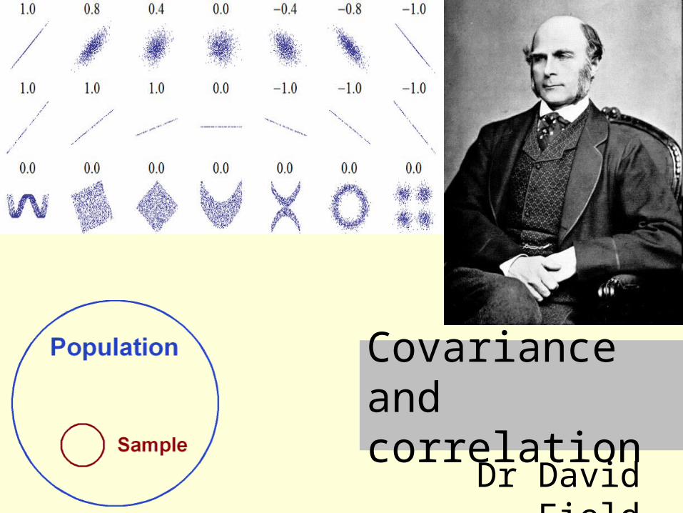
Introduction

• Sometimes it is not possible for researchers to experimentally manipulate an IV using random allocation to conditions and measure a dependent variable – e.g. relationship between income and self esteem

• But you can still measure two or more variables and ask what relationship, if any, they have

• One way to assess this relationship is using the “Pearson product moment correlation”– another example would be to look at the relationship

between alcohol consumption and exam performance in students

– it would be unethical to manipulate alcohol intake

• For each participant we record units of alcohol consumed per week and exam %

• Don’t forget that this is not an experiment, and any observed dependence of the 2 variables on each other could be due to both variables being caused by a 3rd variable (e.g. stress)

• Before performing any statistical analysis the first step is to visualise the relationship between the two variables using a scatter plot.

Units alcohol per

week Exam %

13 63

10 60

24 55

3 70

5 80

35 41

20 50

14 58

17 61

19 63

alcoholExam

%

13 63

10 60

24 55

3 70

5 80

35 41

20 50

14 58

17 61

19 63Scatterplot:

Calculating the covariance of two variables

• Covariance is a measure of how much two variables change together– presumes that for each participant in the sample two variables

have been measured

• If two variables tend to vary together (that is, when one of them is above its mean, then the other variable tends to be above its mean too), then the covariance between the two variables will be positive.

• If, when one of them is above its mean value the other variable tends to be below its mean value, then the covariance between the two variables will be negative.

• First, let’s revisit variance…

Variance of one variable

• To calculate variance– subtract the mean from each score– Square the results– Add up the squared scores– Divide by the number of scores -1

• Squaring makes sure that the variance will not be negative, and it emphasizes the effect of very large and very small scores that are far from the mean

• If all the scores are close to the mean the variable has restricted variance and it is unlikely that any other variable will co-vary with it

Covariance of two variables, X and Y

• For each pair of scores– subtract the mean of variable X from each score in X– subtract the mean of variable Y from each score in Y– Multiply each of the pairs of difference scores together– Sum the results– Divide by the number of scores – 1

• The -1 has negligible effect on the estimate of the population covariance when the sample is large

• But when the sample is small it has a noticeable effect• The -1 is included because it has been shown that small

samples tend to underestimate the underlying population covariance (as is also the case for variance)

alcohol exam %alcohol –

mean (16)

exam – mean (60.1)

Multiply difference

scores

13 63 -3 2.9 -8.7

10 60 -6 -0.1 0.6

24 55 8 -5.1 -40.8

3 70 -13 9.9 -128.7

5 80 -11 19.9 -218.9

35 41 19 -19.1 -362.9

20 50 4 -10.1 -40.4

14 58 -2 -2.1 4.2

17 61 1 0.9 0.9

19 63 3 2.9 8.7

Sum right hand column and divide by number of participants -1 to find the “population” covariance

-786 / 9 = -87.3

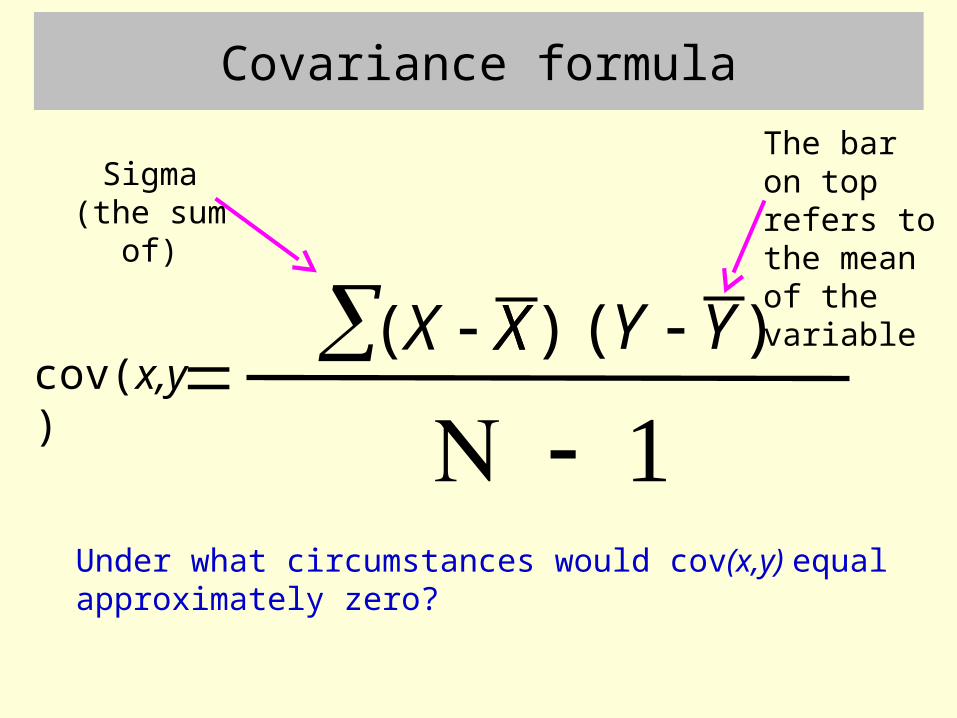
Covariance formula

)( XX

cov(x,y)X )( YY

The bar on top refers to the mean of the variable

Under what circumstances would cov(x,y) equal approximately zero?

Sigma (the sum of)

Converting covariance to correlation

• Knowing that the covariance of two variables is positive is useful as it indicates that as one increases, so does the other

• But, the actual value of covariance is dependent up the measurement units of the variables– if the exam scores had been given out of 45, instead of

as percentages, then the covariance with alcohol consumption would be -39.3 instead of -87.3

– but the real strength of the relationship is the same– because the covariance is dependent upon the

measurement units used it is hard to interpret unless we first standardize it.

Converting covariance to correlation

• Ideally we’d like to be able to ask if the covariation of alcohol consumption and exam scores is stronger or weaker than the covariation of alcohol consumption and hours studied

• The standard deviation provides the answer, because it is a universal unit of measurement into which any other scale of measurement can be converted– because the covariance uses the deviation scores of

two variables, to standardize the covariance we need to make use of the SD of both variables

Pearsons r correlation coefficient

rcov(x,y)

SDx * SDyThis means divide by the

total variation in both variables What is the biggest value r could

take?

Pearsons r correlation coefficient

• The result of standardisation is that r has a minimum of -1 and a maximum of 1– -1 perfect negative relationship– 0 no relationship– 1 perfect positive relationship– -0.5 moderate negative relationship– 0.5 moderate positive relationship

• To achieve a correlation of 1 (or -1) the shared variation, cov(x,y) has to be as big as the total variation in the data, represented by the two SD’s multiplied together

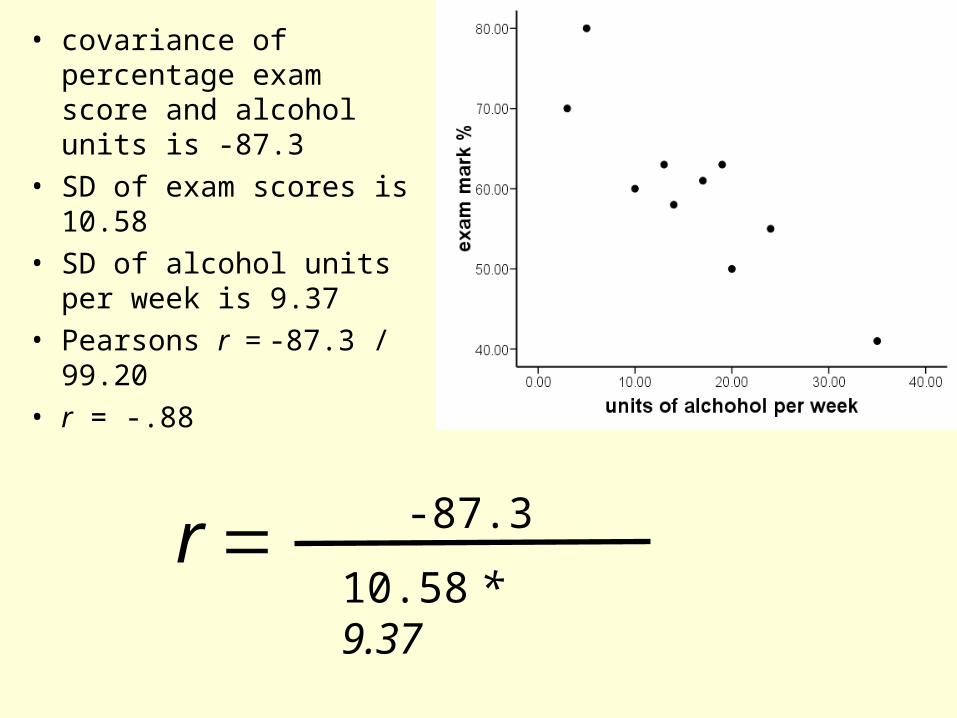
• covariance of percentage exam score and alcohol units is -87.3

• SD of exam scores is 10.58

• SD of alcohol units per week is 9.37

• Pearsons r = -87.3 / 99.20

• r = -.88

r -87.3

10.58 * 9.37

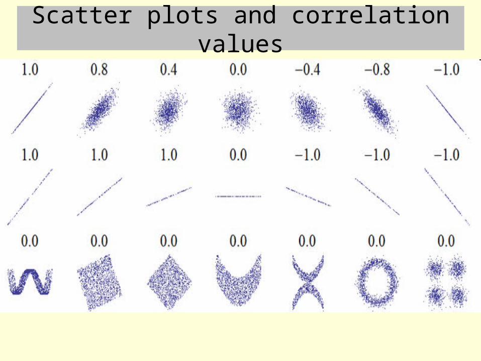
Scatter plots and correlation values

Scatter plots and correlation values

The scatter plot with 0 correlation provides a null hypothesis and null distribution for calculating an inferential statistic.

The correlation coefficient between two variables is itself a descriptive statistic, analogous to the effect size of the difference between two sample means.

We can also calculate the p value of an observed correlation (data) being obtained by random sampling from the null scatter plot.

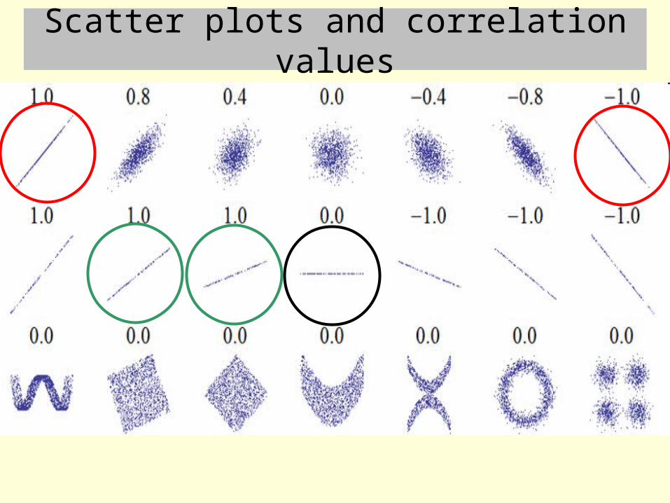
Scatter plots and correlation values

Statistical significance of correlations

• SPSS reports a 2 tailed p value for correlations– this is the probability of obtaining the data by random sampling

from a population scatter plot with 0 correlation– If p is less than 0.05 you can reject the null hypothesis, and declare

the correlation to be statistically significant– if you predicted the direction of correlation, then the p value can be

divided by 2 (one tailed test)

• The p value is very dependent on sample size– if sample size is large then very small values of the correlation

coefficient (e.g. -0.15) will easily reach significance

• Only report correlations that reach significance, but beyond this you should place more emphasis on interpretation of the direction and size of the correlation coefficient itself

The coefficient of determination (R2)

Venn diagrams showing proportion of variance shared between X and Y

0 correlation

Strong (but not perfect) correlation

Weak correlation

The coefficient of determination

• To express quantitatively what is expressed visually by the Venn diagrams– square the correlation coefficient (multiply it by itself)– the result will always be a positive number– it describes the proportion of variance that the two

variables have in common– it is also referred to as R2

0

0.25

0.5

0.75

1

1size of correlation

coe

ffici

en

t of d

ete

rmin

atio

n

00.8 0.6 0.4 0.2

Note the rapid decline of the coefficient as the correlation reduces.

r = 0.9 – 81% shared variance

r = 0.5 – 25% shared variance

r = 0.3 – 9% shared variance

Correlation - limitations

• Before running a correlation between any pair of variables produce a scatter plot in SPSS

• If there is a relationship between the two variables, but it appears to be non-linear, then correlation is not an appropriate statistic– non-linear relationships can be u shaped or n shaped,

or like the graph on the previous slide

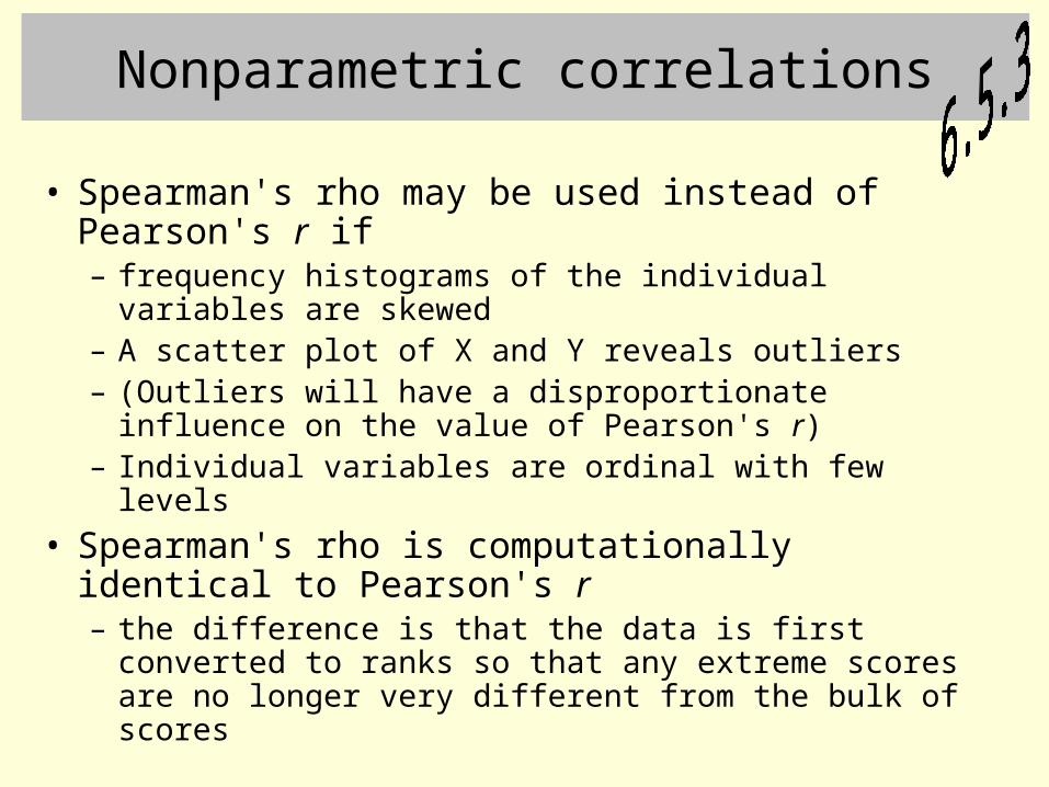
Nonparametric correlations

• Spearman's rho may be used instead of Pearson's r if– frequency histograms of the individual variables are

skewed– A scatter plot of X and Y reveals outliers– (Outliers will have a disproportionate influence on the

value of Pearson's r)– Individual variables are ordinal with few levels

• Spearman's rho is computationally identical to Pearson's r– the difference is that the data is first converted to ranks

so that any extreme scores are no longer very different from the bulk of scores

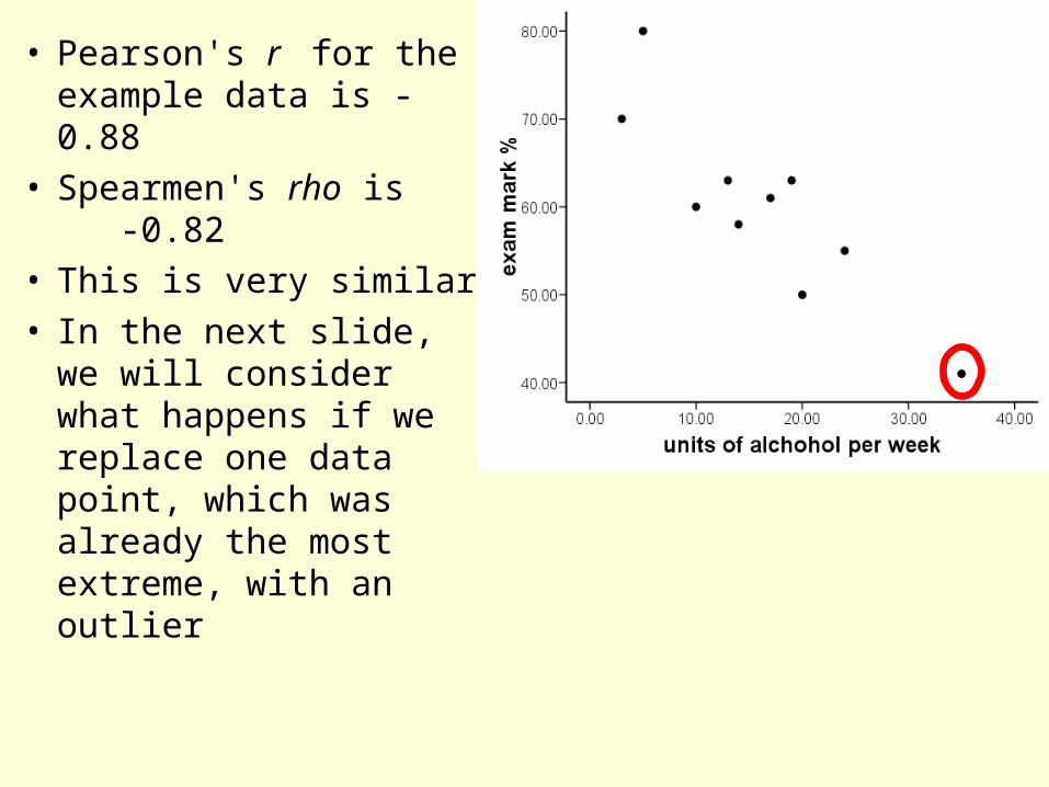
• Pearson's r for the example data is -0.88

• Spearmen's rho is -0.82

• This is very similar• In the next slide, we

will consider what happens if we replace one data point, which was already the most extreme, with an outlier

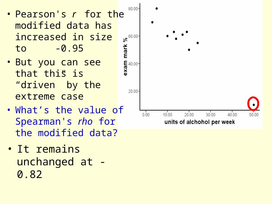
• Pearson's r for the modified data has increased in size to -0.95

• But you can see that this is “driven” by the extreme case

• What’s the value of Spearman's rho for the modified data?

• It remains unchanged at -0.82

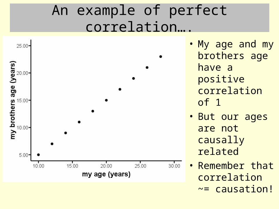
An example of perfect correlation….

• My age and my brothers age have a positive correlation of 1

• But our ages are not causally related

• Remember that correlation ~= causation!