Course Notes v17
82
Part I Speech Processing 1 In tr oduction Speech Processing: 1. Speec h/Speak er Recognition 2. Syn thesi s 3. Speec h Coding (Communication) In this course: 1. Analy sis (Modeling, Physio logy) (a) Time domain (b) Frequency domain 2. Coding 2 Review of Digital Signal Pr oces sing Fundamentals 2.1 Discre te- Time Signals Speech signals occur naturally as continuous-time acoustic signals, x a (t). How ev er, speech signals can be transduced into electrical signals, and sampled at period T = 1/F s to become discrete-time signals or sequences: x (n) = x a (t) t=nT = x a (nT ) . • Sampling Theorem: Let x a (t) be a continuous-time signal, and let X a ( ) be the corresponding frequency representation. Suppose x a (t) is bandlimited: x a ( ) = 0 , for | | > a , where a = 2πF a . If x a (t) is sampled at period T = 1/F s to become x (n), then x a (t) can be uniquely reconstructed from x (n) if F s > 2F a . Here, F a is referred to as the bandwidth of x a (t). The Nyquist rate is defined as F N = 2F a . If the original continuous-time signal is not band-limited, the sampling component must be preceded by a low-pass filter with cut-off frequency F c ≤ F s 2 in order to avoid aliasing. Note that speech signa ls are typical ly not band-limited. Ho wev er, the majorit y of useful infor mati on is contained below certain frequencies. For example, for speech coding, speech is generally sampled at 8kHz (narrowband coding) or 16 kHz (wideband coding). For music, the sampling rate is generally much higher, such as 44.1kHz or PCM coded music. 1
description
UCLA EE114 Coursereader
Transcript of Course Notes v17
7/18/2019 Course Notes v17
http://slidepdf.com/reader/full/course-notes-v17 1/82
Part I
Speech Processing
1 Introduction
Speech Processing:
1. Speech/Speaker Recognition
2. Synthesis
3. Speech Coding (Communication)
In this course:
1. Analysis (Modeling, Physiology)
(a) Time domain
(b) Frequency domain
2. Coding
2 Review of Digital Signal Processing Fundamentals
2.1 Discrete-Time Signals
Speech signals occur naturally as continuous-time acoustic signals, xa (t). However, speech signals canbe transduced into electrical signals, and sampled at period T = 1/F s to become discrete-time signals orsequences:
x (n) = xa (t)t=nT = xa (nT ) .
• Sampling Theorem: Let xa (t) be a continuous-time signal, and let X a ( ) be the correspondingfrequency representation. Suppose xa (t) is bandlimited:
xa ( ) = 0, for | | > a,
where a = 2πF a. If xa (t) is sampled at period T = 1/F s to become x (n), then xa (t) can beuniquely reconstructed from x (n) if F s > 2F a. Here, F a is referred to as the bandwidth of xa(t). The
Nyquist rate is defined as F N = 2F a.
If the original continuous-time signal is not band-limited, the sampling component must be preceded
by a low-pass filter with cut-off frequency F c ≤ F s
2 in order to avoid aliasing.
Note that speech signals are typically not band-limited. However, the majority of useful information is
contained below certain frequencies. For example, for speech coding, speech is generally sampled at 8kHz(narrowband coding) or 16 kHz (wideband coding). For music, the sampling rate is generally much higher,
such as 44.1 kHz or PCM coded music.
1
7/18/2019 Course Notes v17
http://slidepdf.com/reader/full/course-notes-v17 2/82
2.2 Important Discrete-Time Functions
Several discrete-time functions are important to digital speech processing, and will be used repeatedly inthis course:
• The delta function: x (n) = δ (n)
x (n) = 1, for n = 0,
0, otherwise.
• The step function: x (n) = u (n)
x (n) =
1, for n ≥ 0,0, otherwise.
• The one-sided exponential function: x (n) = an u (n)
x (n) =
an, for n ≥ 0,0, otherwise.
• Sinusoidal functions:
x (n) = cos(2πf n),x (n) = sin(2πf n).
• Euler’s Identity: e jθn = cos (θn) + j sin (θn).⇒ Note that Euler’s Identity can be used to expand sinusoidal functions:cos(θn) = 1
2
e jθn + e− jθn
,
sin(θn) = 12j
e jθn − e− jθn
.
2.3 Important Discrete-Time Frequency-Domain Transforms
Frequency-domain transforms allow for spectral analysis of signals and systems. In this section, severalcommon discrete-time transforms will be reviewed:
• The Z-transform expresses an input signal x (n) as a geometric series in the complex variable z = re jω:
X (z) =∞
n=−∞x (n) z−n.
An important topic regarding the Z-transform is the region of convergence (ROC), which is definedas all portions of the Z-plane for which:
∞
n=−∞|x (n) z−n| =
∞
n=−∞|x (n) r−ne− jnω| =
∞
n=−∞|x (n) r−n| < ∞.
Note that different discrete-time signals may have the same Z-transform, but different ROCs (e.g.,
x1(n) = anu(n) and x2(n) = −anu(−n − 1)).
The inverse Z-transform allows the time-domain signal to be obtained from the transform-domain
representation:
x (n) = 1
2π j
C
X (z) zn−1 dz,
2
7/18/2019 Course Notes v17
http://slidepdf.com/reader/full/course-notes-v17 3/82
where C denotes a path surrounding the origin and contained in the ROC.
• The Discrete-Time Fourier Transform (DTFT) expresses an input signal as a geometric series in the
complex variable e jω:
X e jω
=∞
n=−∞x (n) e− jωn.
The DTFT represents a transformation from discrete time, n, to continuous frequency, ω. Bydefinition, the DTFT is periodic in frequency (ω) with period 2π. The inverse DTFT allows thetime-domain signal to be obtained from the frequency-domain representation:
x (n) = 1
2π
π
−π
X
e jω
e jωn dω.
Note that the DTFT can be interpreted as the Z-transform evaluated along the unit circle (|z| = 1):
X e jω = X (z)z=e
jω .
• The N -point Discrete Fourier Transform (DFT) provides a discrete frequency representation of afinite length discrete-time signal x (n) of length L ≤ N :
X (k) =L−1n=0
x (n) e− j 2πN kn , for 0 ≤ k ≤ N − 1.
The DFT represents a transformation from discrete time, n, to discrete frequency, k. Note that thelength of the sequence is not required to be equal to the size of the DFT, as long as L ≤ N . If L < N ,the sequence is said to be zero-padded with N − L zeros. The discrete frequency representationgiven by the DFT is at many times easier to handle in practice than the continuous representation
provided by the DTFT.
Note that the DFT assumes implicit periodicity of period N , both in the time and frequency domain.
The inverse DFT is given by:
x (n) = 1
N
N −1k=0
X (k) e j 2πN kn , for 0 ≤ n ≤ N − 1.
Note also that the DFT can be interpreted as a uniform sampling of the DTFT along the unit circle:
X (k) = X e jω
ω= 2πkN
.
There exist computationally efficient algorithms for determining the DFT, namely the Fast FourierTransforms (FFTs), many of which require the length of the input time-domain signal to be a power
of 2. Since this is not generally the case, time signals may be zero-padded to produce lengths of 2v
(also known as radix-2).
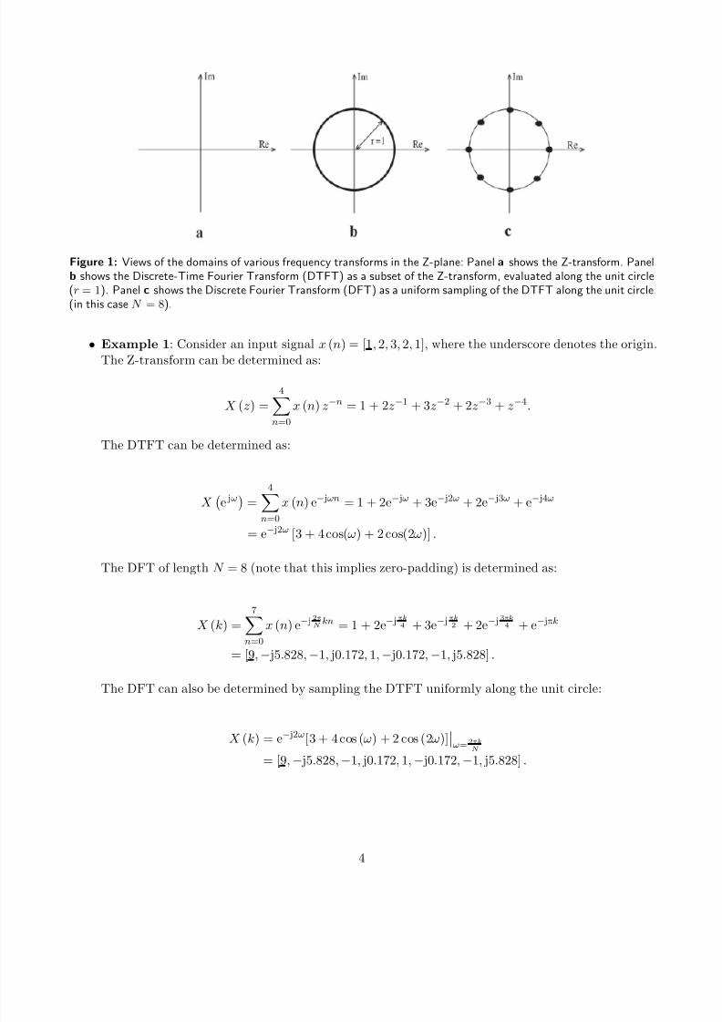
Figure 1 provides views of the domains of the transforms previously discussed, in the Z-plane.
3
7/18/2019 Course Notes v17
http://slidepdf.com/reader/full/course-notes-v17 4/82
Figure 1: Views of the domains of various frequency transforms in the Z-plane: Panel a shows the Z-transform. Panelb shows the Discrete-Time Fourier Transform (DTFT) as a subset of the Z-transform, evaluated along the unit circle(r = 1). Panel c shows the Discrete Fourier Transform (DFT) as a uniform sampling of the DTFT along the unit circle(in this case N = 8).
• Example 1: Consider an input signal x (n) = [1, 2, 3, 2, 1], where the underscore denotes the origin.
The Z-transform can be determined as:
X (z) =4
n=0
x (n) z−n = 1 + 2z−1 + 3z−2 + 2z−3 + z−4.
The DTFT can be determined as:
X
e jω
=4
n=0
x (n) e− jωn = 1 + 2e− jω + 3e− j2ω + 2e− j3ω + e− j4ω
= e− j2ω
[3 + 4 cos(ω) + 2 cos(2ω)] .
The DFT of length N = 8 (note that this implies zero-padding) is determined as:
X (k) =7
n=0
x (n) e− j 2πN kn = 1 + 2e− j πk
4 + 3e− j πk2 + 2e− j 3πk
4 + e− jπk
= [9, − j5.828, −1, j0.172, 1, − j0.172, −1, j5.828] .
The DFT can also be determined by sampling the DTFT uniformly along the unit circle:
X (k) = e− j2ω[3 + 4 cos (ω) + 2 cos (2ω)]ω= 2πk
N
= [9, − j5.828, −1, j0.172, 1, − j0.172, −1, j5.828] .
4
7/18/2019 Course Notes v17
http://slidepdf.com/reader/full/course-notes-v17 5/82
2.4 Properties of Frequency-Domain Transforms
There exist several important properties pertaining to frequency-domain transforms of discrete-time signals
that assist in the analysis of signals and systems. Note that if the properties discussed in this sectionapply identically to all transforms previously discussed, they will only be explicitly formalized for theDFT, for the sake of brevity. However, differences occur, the properties will be formalized separately for
each necessary transform.
• Linearity:Let x1 (n) and x2 (n) be time-domain signals, with X 1 (k) and X 2 (k) being the corresponding DFTs:
x1 (n) ↔ X 1 (k) ,
x2 (n) ↔ X 2 (k) .
In this case, a linear combination of the time-domain signals will produce a linear combination of the frequency-domain signals:
αx1 (n) + βx2 (n)
↔αX 1 (k) + βX 2 (k) .
One subtle aspect of the linearity property is when dealing with time-domain signals of variouslengths, say N 1 and N 2, they must be initially zero-padded to at least length N = max(N 1, N 2) toavoid aliasing in the time domain.
• Convolution:Convolution of signals in the time-domain results in multiplication of corresponding signals in the
frequency domain. Conversely, multiplication in the time domain results in convolution in thefrequency domain. For the DTFT, this property refers to standard convolution, denoted by ∗:
x1 (n) ∗ x2 (n) ↔ X 1 e jω
X 2 e jω
,
x1 (n) x2 (n) ↔ 12π
X 1
e jω ∗ X 2
e jω .
However, due to the implied periodicity of the DFT, this property refers to circular convolution,denoted by , in this case:
x1 (n) x2 (n) ↔ X 1 (k) X 2 (k) ,
x1 (n) x2 (n) ↔ 1
N X 1 (k) X 2 (k) .
• Time-Shifts:Introducing a time shift results in modulation in the frequency domain by a complex exponential.For the DTFT, this refers to a standard time shift:
x (n − no) ↔ e− jnoωX
e jω
.
However, for the DFT, due to the implied periodicity, this refers to a modular time shift:
x ((n − no)mod N ) ↔ e− j2πknoN X (k) .
5
7/18/2019 Course Notes v17
http://slidepdf.com/reader/full/course-notes-v17 6/82
• Real Time-Domain Signals:Real time-domain signals will results in frequency-domain transforms which are conjugate symmetric.
That is:
x (n) ≡ real ↔ X (k) = X ∗ (−k mod N ) .
This property is important for speech processing since speech signals are naturally real.
2.5 Insight Into Discrete-Time Frequencies
For continuous-time signals, frequencies can take values within the entire range (−∞, ∞). Generally,continuous-time frequencies are denoted (radians per second) or F (hertz). However, as can be interpreted
from the sampling theorem previously discussed, sampling limits the range of possible frequency components
in a signal. For a discrete-time signal, frequencies are generally denoted by ω (radians per sample), which
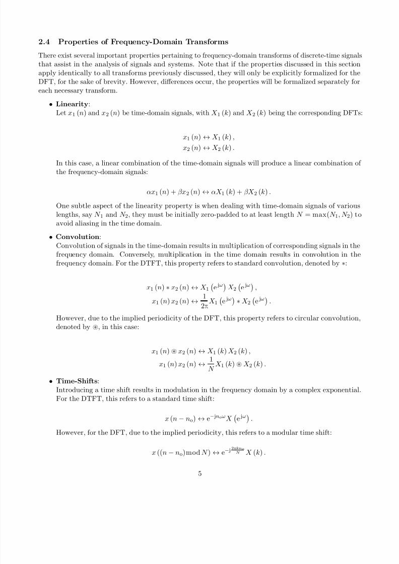
take values within [0, 2π). Figure 2 provides examples of unit amplitude discrete-time signals at variousfrequencies.
1 2 3 4 5 6 7 8 9 10
−1
0
1
1 2 3 4 5 6 7 8 9 10
−1
0
1
1 2 3 4 5 6 7 8 9 10
−1
0
1
a
b
c
Figure 2: Examples of Discrete-Time Frequencies: Panel a shows a unit-amplitude signal of frequency ω = 0. Panel bshows a unit-amplitude signal of frequency ω = π
2. Panel c shows a unit-amplitude signal of frequency ω = π, which is
the highest possible frequency. Note that the phase is zero in each case.
The relationship between discrete-time frequencies and corresponding continuous-time frequencies is
dependent on the sampling frequency, F s:
ω =
F s.
6
7/18/2019 Course Notes v17
http://slidepdf.com/reader/full/course-notes-v17 7/82
Furthermore, when the DFT is used for spectral analysis, the spacing between frequency bins is givenas:
∆ω = 2π
N .
• Example 2:
Let x (n) be a discrete-time signal with sampling rate F s = 8kHz. If a segment of the signalcorresponding to 25ms is extracted for spectral analysis, and a radix-2 FFT is to be used, what is
the minimum length N of the signal used (after zero-padding) during the transform?
A signal of duration T = 25 ms with sampling rate F s comprises:
N = 0.025s × 8000 samples/s = 200 samples.
However, since the length of the signal must of the form 2v, the final length of the signal after zeropadding should be:
ν = log2(N ) = 8 → N FFT = 28 = 256 samples.
• Example 3:Let x (n) be a discrete-time signal with sampling rate F s = 8kHz. A segment of the signalcorresponding to 25ms is extracted for spectral analysis. If the DFT is used for spectral analysis,what is the minimum length, N , of signal used in order to provide frequency resolution ∆F ≤ 20Hz?
(In this case, don’t worry about using FFTs.)
Note that the minimum frequency resolution is given in the continuous-frequency domain, so thediscrete-frequency resolution must be determined:
∆ω = ∆
F s=
2π∆F
F s≤ 0.005π.
The frequency resolution provided by the DFT is given by ∆ω = 2π
N , so the minimum signal lengthcan be determined as:
2π
N ≤ 0.005π ⇒ N ≥ 400 samples.
The minimum length of the discrete signal, after zero-padding, to guarantee frequency resolution of 20 Hz is N = 400 samples.
2.6 Linear Time-Invariant Systems
The properties of linearity and time-invariance greatly simplify the analysis of systems. Consider the
system:
x(n) −→ H (z) −→ y(n)
Here, Y (Z ) = H (z) X (z), and y (n) is determined as:
y (n) = (h ∗ x) (n) =∞
m=−∞h (m) x (n − m) ,
7
7/18/2019 Course Notes v17
http://slidepdf.com/reader/full/course-notes-v17 8/82
where h (n) is the impulse response. Note that if the system applies the DFT, circular convolution () isused instead. To make the outputs of standard and circular convolution equivalent, the size of the DFT
needs to chosen as N ≥ N 1 + N 2 − 1, where N 1 and N 2 are the lengths of the signals being convolved.Systems comprise zeros and poles (which will be discussed later during the topic of speech production).Zeros and poles are characterized by a spectral location as well as a bandwidth. The effect of zeros areattenuations in the frequency response, whereas the effect of poles are gains in the frequency response.
• Linearity:Let x1 (n) and x2 (n) be input signals, and let y1 (n) and y2 (n) be corresponding output signals. If the system H (z) is linear, then:
αx1 (n) + βx2 (n) → αy1 (n) + βy2 (n) .
• Time Invariance:The property of time-invariance describes a system H (z) as remaining constant throughout time. If
H (z) is time-invariant, then:
x (n−
no)→
y (n−
no) .
As will be seen later in the course, the speech production system is highly time-varying. However,aspects of the speech production system can be sampled at high enough rates to allow the assumption
of stationarity and thus assume time-invariance.
If a system is LTI, then the transfer function H (z), or equivalently the impulse response h (n),completely characterizes the system.
Additionally, systems that are in series can be combined to form a single cascaded system:
x(n) −→ H 1(z) −→ H 2(z) −→ y(n) =⇒ x(n) −→ H (z) −→ y(n)
where H (z) = H 1 (z) H 2 (z), or equivalently, h (n) = (h1
∗h2) (n).
8
7/18/2019 Course Notes v17
http://slidepdf.com/reader/full/course-notes-v17 9/82
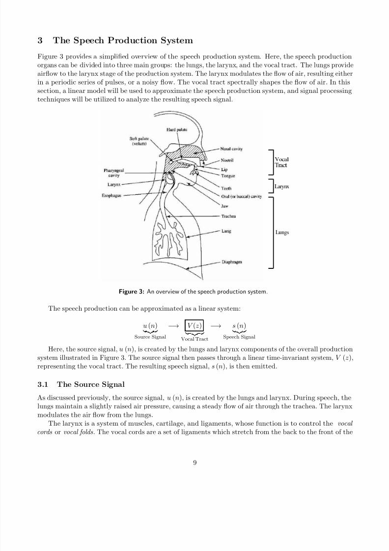
3 The Speech Production System
Figure 3 provides a simplified overview of the speech production system. Here, the speech productionorgans can be divided into three main groups: the lungs, the larynx, and the vocal tract. The lungs provide
airflow to the larynx stage of the production system. The larynx modulates the flow of air, resulting either
in a periodic series of pulses, or a noisy flow. The vocal tract spectrally shapes the flow of air. In thissection, a linear model will be used to approximate the speech production system, and signal processing
techniques will be utilized to analyze the resulting speech signal.
Figure 3: An overview of the speech production system.
The speech production can be approximated as a linear system:
u (n) Source Signal
−→ V (z) Vocal Tract
−→ s (n) Speech Signal
Here, the source signal, u (n), is created by the lungs and larynx components of the overall production
system illustrated in Figure 3. The source signal then passes through a linear time-invariant system, V (z),
representing the vocal tract. The resulting speech signal, s (n), is then emitted.
3.1 The Source SignalAs discussed previously, the source signal, u (n), is created by the lungs and larynx. During speech, thelungs maintain a slightly raised air pressure, causing a steady flow of air through the trachea. The larynx
modulates the air flow from the lungs.The larynx is a system of muscles, cartilage, and ligaments, whose function is to control the vocal
cords or vocal folds . The vocal cords are a set of ligaments which stretch from the back to the front of the
9
7/18/2019 Course Notes v17
http://slidepdf.com/reader/full/course-notes-v17 10/82
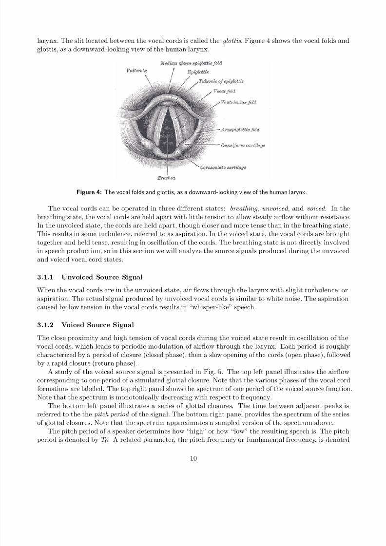
larynx. The slit located between the vocal cords is called the glottis . Figure 4 shows the vocal folds and
glottis, as a downward-looking view of the human larynx.
Figure 4: The vocal folds and glottis, as a downward-looking view of the human larynx.
The vocal cords can be operated in three different states: breathing , unvoiced , and voiced . In thebreathing state, the vocal cords are held apart with little tension to allow steady airflow without resistance.
In the unvoiced state, the cords are held apart, though closer and more tense than in the breathing state.This results in some turbulence, referred to as aspiration. In the voiced state, the vocal cords are brought
together and held tense, resulting in oscillation of the cords. The breathing state is not directly involvedin speech production, so in this section we will analyze the source signals produced during the unvoiced
and voiced vocal cord states.
3.1.1 Unvoiced Source Signal
When the vocal cords are in the unvoiced state, air flows through the larynx with slight turbulence, oraspiration. The actual signal produced by unvoiced vocal cords is similar to white noise. The aspiration
caused by low tension in the vocal cords results in “whisper-like” speech.
3.1.2 Voiced Source Signal
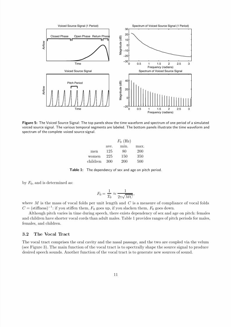
The close proximity and high tension of vocal cords during the voiced state result in oscillation of thevocal cords, which leads to periodic modulation of airflow through the larynx. Each period is roughlycharacterized by a period of closure (closed phase), then a slow opening of the cords (open phase), followed
by a rapid closure (return phase).A study of the voiced source signal is presented in Fig. 5. The top left panel illustrates the airflow
corresponding to one period of a simulated glottal closure. Note that the various phases of the vocal cordformations are labeled. The top right panel shows the spectrum of one period of the voiced source function.
Note that the spectrum is monotonically decreasing with respect to frequency.The bottom left panel illustrates a series of glottal closures. The time between adjacent peaks is
referred to the the pitch period of the signal. The bottom right panel provides the spectrum of the seriesof glottal closures. Note that the spectrum approximates a sampled version of the spectrum above.
The pitch period of a speaker determines how “high” or how “low” the resulting speech is. The pitchperiod is denoted by T 0. A related parameter, the pitch frequency or fundamental frequency, is denoted
10
7/18/2019 Course Notes v17
http://slidepdf.com/reader/full/course-notes-v17 11/82
!"#$
% " & ' ( ) *
+)",$- /)0&,$ /"123( 45 6$&")-7
8 89: 5 59: ; ;9: <<8
;8
58
8
58
;8
<8
=&$>0$2,? 4&3-"32@7
A 3 1 2 " B 0 - $ 4 - C 7
/D$,B&0# )' +)",$- /)0&,$ /"123( 45 6$&")-7
!"#$
% " & ' ( ) *
+)",$- /)0&,$ /"123(
8 89: 5 59: ; ;9: <;8
8
;8
E8
=&$>0$2,? 4&3-"32@7
A 3 1 2 " B 0 - $ 4 - C 7
/D$,B&0# )' +)",$- /)0&,$ /"123(
6"B,F 6$&")-
G()@$- 6F3@$ HD$2 6F3@$ I$B0&2 6F3@$
Figure 5: The Voiced Source Signal: The top panels show the time waveform and spectrum of one period of a simulatedvoiced source signal. The various temporal segments are labeled. The bottom panels illustrate the time waveform andspectrum of the complete voiced source signal.
F 0 (Hz)ave. min. max.
men 125 80 200women 225 150 350
children 300 200 500
Table 1: The dependency of sex and age on pitch period.
by F 0, and is determined as:
F 0 = 1
T 0≈ 1
2π√
MC ,
where M is the mass of vocal folds per unit length and C is a measure of compliance of vocal foldsC = (stiffness)−1: if you stiffen them, F 0 goes up, if you slacken them, F 0 goes down.
Although pitch varies in time during speech, there exists dependency of sex and age on pitch: females
and children have shorter vocal cords than adult males. Table 1 provides ranges of pitch periods for males,
females, and children.
3.2 The Vocal Tract
The vocal tract comprises the oral cavity and the nasal passage, and the two are coupled via the velum(see Figure 3). The main function of the vocal tract is to spectrally shape the source signal to producedesired speech sounds. Another function of the vocal tract is to generate new sources of sound.
11
7/18/2019 Course Notes v17
http://slidepdf.com/reader/full/course-notes-v17 12/82
3.2.1 Spectral Shaping
It is commonly assumed that the relationship between the source signal airflow and the airflow outputted
by the vocal tract can be approximated by a linear filter, V (z). Certain configurations of the vocaltract components create specific resonant frequencies, referred to as formant frequencies or formants , and
denoted by F i. Note that the term formant can refer to information regarding both the spectral locationand bandwidth of the corresponding resonance. In terms of the expression for H (z), the energy gain
present for formants is due to p poles. Since speech is naturally a real signal, the vocal tract transferfunction’s poles are either real or complex conjugate pairs:
V (z) = G
p1/2k=1
(1 − ckz−1)
1 − c∗kz−1 p2=1
(1 − rz−1)
, p = p1 + p2.
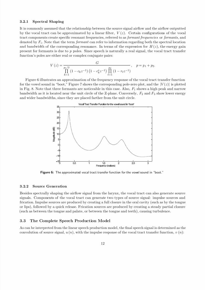
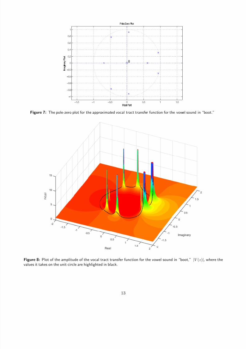
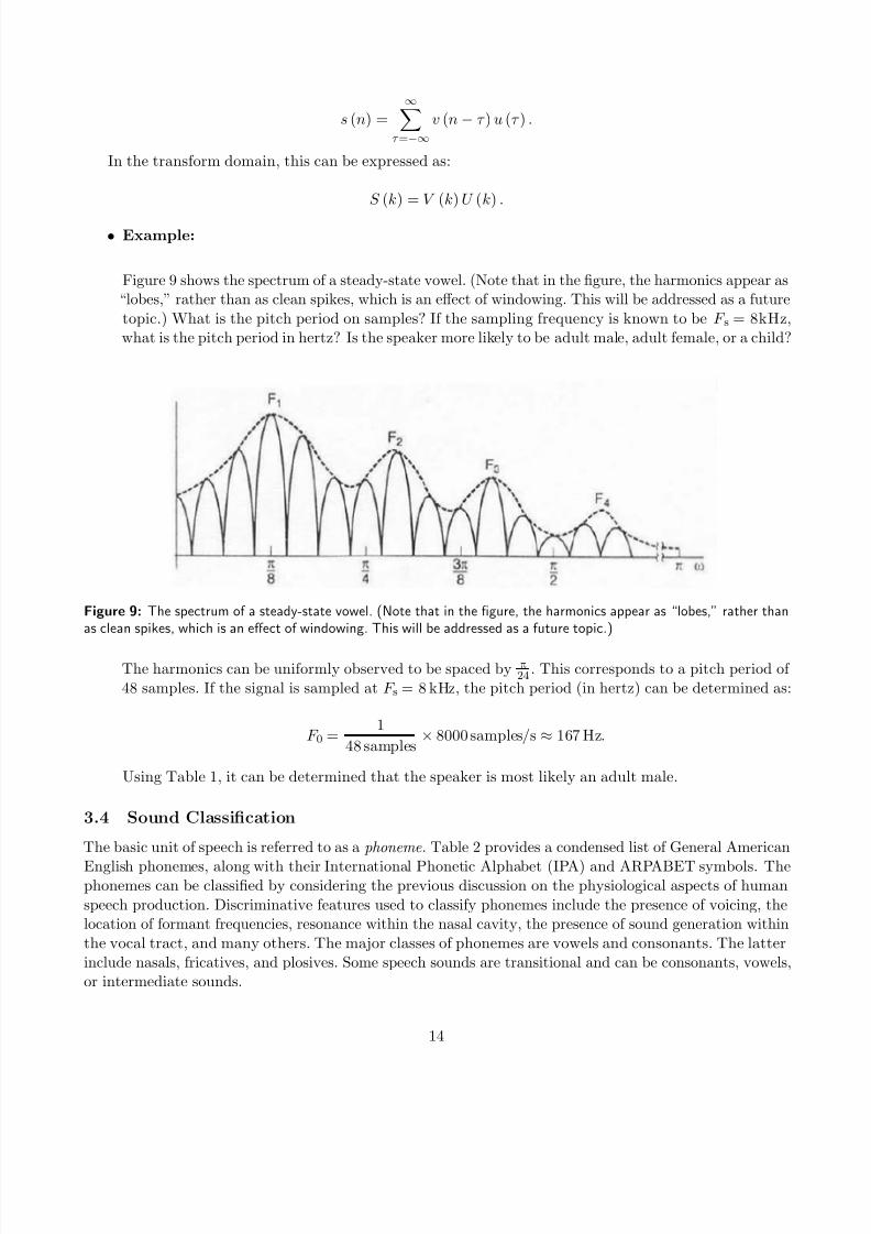
Figure 6 illustrates an approximation of the frequency response of the vocal tract transfer functionfor the vowel sound in “boot,” Figure 7 shows the corresponding pole-zero plot, and the |V (z)| is plottedin Fig. 8. Note that three formants are noticeable in this case. Also, F 1 shows a high peak and narrowbandwidth as it is located near the unit circle of the Z-plane. Conversely, F 2 and F 3 show lower energyand wider bandwidths, since they are placed farther from the unit circle.
Figure 6: The approximated vocal tract transfer function for the vowel sound in “boot.”
3.2.2 Source Generation
Besides spectrally shaping the airflow signal from the larynx, the vocal tract can also generate sourcesignals. Components of the vocal tract can generate two types of source signal: impulse sources and
frication. Impulse sources are produced by creating a full closure in the oral cavity (such as by the tongueor lips), followed by a quick release. Frication sources are produced by creating a steady partial closure(such as between the tongue and palate, or between the tongue and teeth), causing turbulence.
3.3 The Complete Speech Production Model
As can be interpreted from the linear speech production model, the final speech signal is determined as the
convolution of source signal, u (n), with the impulse response of the vocal tract transfer function, v (n):
12
7/18/2019 Course Notes v17
http://slidepdf.com/reader/full/course-notes-v17 13/82
Figure 7: The pole-zero plot for the approximated vocal tract transfer function for the vowel sound in “boot.”
Figure 8: Plot of the amplitude of the vocal tract transfer function for the vowel sound in “boot,” |V (z)|, where thevalues it takes on the unit circle are highlighted in black.
13
7/18/2019 Course Notes v17
http://slidepdf.com/reader/full/course-notes-v17 14/82
s (n) =
∞τ =−∞
v (n − τ ) u (τ ) .
In the transform domain, this can be expressed as:
S (k) = V (k) U (k) .
• Example:
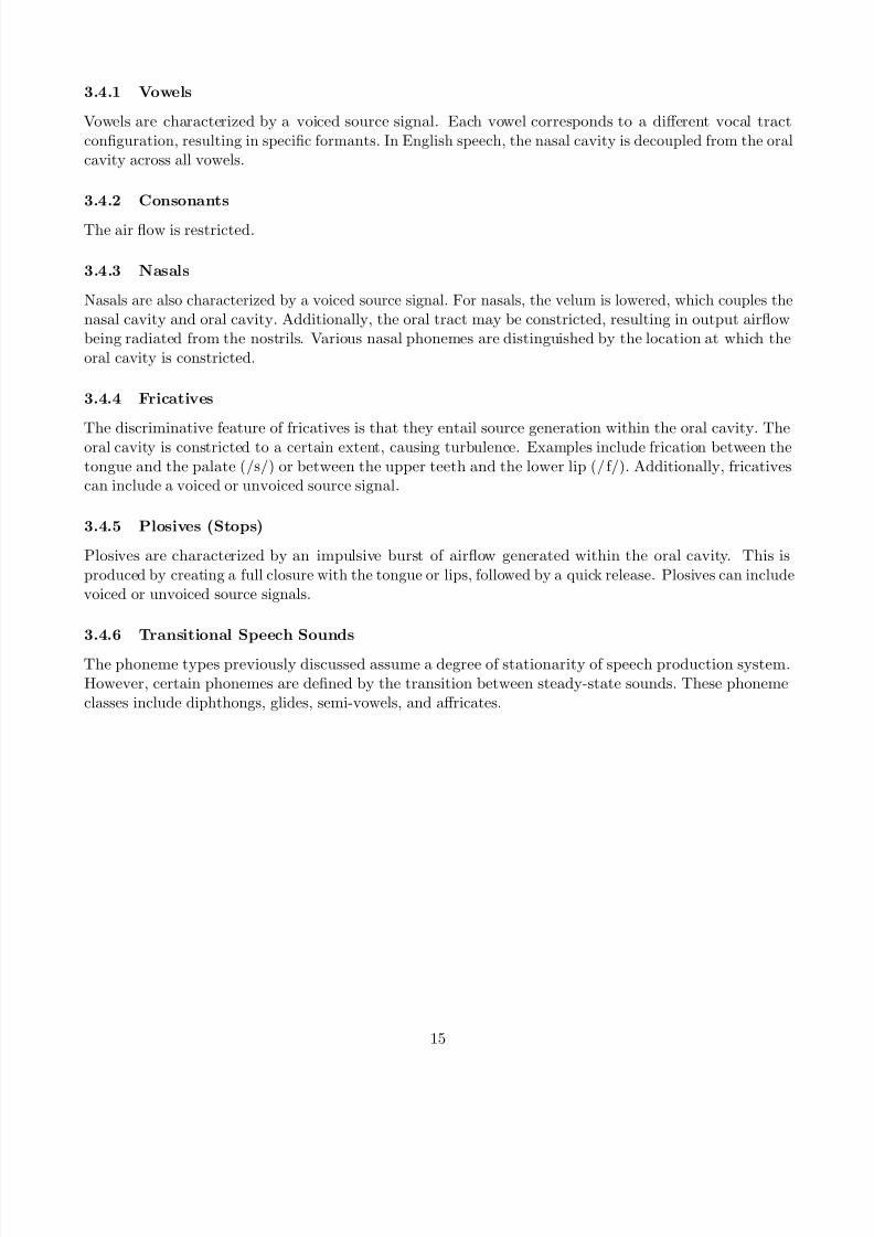
Figure 9 shows the spectrum of a steady-state vowel. (Note that in the figure, the harmonics appear as“lobes,” rather than as clean spikes, which is an effect of windowing. This will be addressed as a future
topic.) What is the pitch period on samples? If the sampling frequency is known to be F s = 8kHz,what is the pitch period in hertz? Is the speaker more likely to be adult male, adult female, or a child?
Figure 9: The spectrum of a steady-state vowel. (Note that in the figure, the harmonics appear as “lobes,” rather thanas clean spikes, which is an effect of windowing. This will be addressed as a future topic.)
The harmonics can be uniformly observed to be spaced by π
24 . This corresponds to a pitch period of
48 samples. If the signal is sampled at F s = 8 kHz, the pitch period (in hertz) can be determined as:
F 0 = 1
48 samples × 8000 samples/s ≈ 167 Hz.
Using Table 1, it can be determined that the speaker is most likely an adult male.
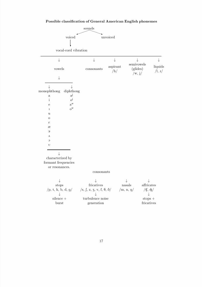
3.4 Sound Classification
The basic unit of speech is referred to as a phoneme . Table 2 provides a condensed list of General American
English phonemes, along with their International Phonetic Alphabet (IPA) and ARPABET symbols. Thephonemes can be classified by considering the previous discussion on the physiological aspects of human
speech production. Discriminative features used to classify phonemes include the presence of voicing, thelocation of formant frequencies, resonance within the nasal cavity, the presence of sound generation within
the vocal tract, and many others. The major classes of phonemes are vowels and consonants. The latter
include nasals, fricatives, and plosives. Some speech sounds are transitional and can be consonants, vowels,
or intermediate sounds.
14
7/18/2019 Course Notes v17
http://slidepdf.com/reader/full/course-notes-v17 15/82
3.4.1 Vowels
Vowels are characterized by a voiced source signal. Each vowel corresponds to a different vocal tractconfiguration, resulting in specific formants. In English speech, the nasal cavity is decoupled from the oral
cavity across all vowels.
3.4.2 Consonants
The air flow is restricted.
3.4.3 Nasals
Nasals are also characterized by a voiced source signal. For nasals, the velum is lowered, which couples the
nasal cavity and oral cavity. Additionally, the oral tract may be constricted, resulting in output airflowbeing radiated from the nostrils. Various nasal phonemes are distinguished by the location at which the
oral cavity is constricted.
3.4.4 Fricatives
The discriminative feature of fricatives is that they entail source generation within the oral cavity. Theoral cavity is constricted to a certain extent, causing turbulence. Examples include frication between thetongue and the palate (/s/) or between the upper teeth and the lower lip (/f /). Additionally, fricativescan include a voiced or unvoiced source signal.
3.4.5 Plosives (Stops)
Plosives are characterized by an impulsive burst of airflow generated within the oral cavity. This isproduced by creating a full closure with the tongue or lips, followed by a quick release. Plosives can include
voiced or unvoiced source signals.
3.4.6 Transitional Speech Sounds
The phoneme types previously discussed assume a degree of stationarity of speech production system.However, certain phonemes are defined by the transition between steady-state sounds. These phonemeclasses include diphthongs, glides, semi-vowels, and affricates.
15

7/18/2019 Course Notes v17
http://slidepdf.com/reader/full/course-notes-v17 16/82
Phoneme ARPABET Example Phoneme ARPABET Example
/i/ IY beat /N/ NG sing
/I/ IH bit /p/ P pet/e j/ EY bait /t/ T ten/E/ EH bet /k/ K kit/æ/ AE bat /b/ B bet/a/ AA bob /d/ D debt
/2/ AH but /g/ G get/O/ AO bought /h/ HH hat
/ow/ OW boat /f / F fat/Ú/ UH book /T/ TH thing/u/ UW boot /s/ S sat/@/ AX about / S / SH shut/1/ IX roses /v/ V vat/Ç / ER bird /D/ DH that/Ä/ AXR butter /z/ Z zoo
/aw/ AW down /Z/ ZH azure/a j/ AY bite /Ù / CH church/O j/ OY boy /Ã/ JH judge
/ j/ Y you /û/ WH which/w/ W wit /ł
"/ EL battle
/ô/ R rent /m"
/ EM bottom/l/ L let /n
"/ EN button
/m/ M met /R/ DX batter/n/ N net /P/ Q (glottal stop)
Table 2: Condensed IPA and ARPABET lists for General American English.
16
7/18/2019 Course Notes v17
http://slidepdf.com/reader/full/course-notes-v17 17/82
Possible classification of General American English phonemes
vocal-cord vibration
voiced unvoiced
sounds
↓ ↓ ↓ ↓ ↓
vowels consonants aspirant
/h/
semivowels(glides)/w, j/
liquids/l, ô/
↓
↓ ↓monophthong diphthong
a a j
i e j
e aw
I ow
u
o
E
æ
Ç
2
O
Ú
↓characterized by
formant frequenciesor resonances.
consonants
↓ ↓ ↓ ↓stops
/p, t, k, b, d, g/fricatives
/s, S , z, Z, v, f , T, D/nasals
/m, n, N/affricates
/Ù , Ã/↓ ↓ ↓
silence +burst
turbulence noisegeneration
stops +fricatives
17
7/18/2019 Course Notes v17
http://slidepdf.com/reader/full/course-notes-v17 18/82
4 Tube Model of the Vocal Tract
How can one find the transfer function V (z)?
Wave equations:
−∂u(x,t)
∂x =A
ρc2∂p(x,t)
∂t
−∂p(x,t)
∂x =
ρ
A
∂u(x,t)
∂twhere
A = cross-sectional area (assumed uniform)t = timeρ = 1.14 × 10⁻³ g cm−3
volume velocity u =0cm3/s to 1000cm3/sc ≈ 340 m/s to 350m/s in air p = pressure.
The pressure is usually given in terms of the sound pressure level, SPL, in dB:
SPL = 20 log P rms
P ref ,
where P ref = 20 µPa is the reference pressure, considered to be the audibility threshold for humans at1 kHz.
Note that in the equations above we can draw parallels to electric circuits by making the followinganalogies:
Acoustic quantity Analogous electric quantity
p, pressure v, voltageu, velocity i, currentρ/A, acoustic inductance L, inductanceA/(ρc2), acoustic capacitance C , capacitance
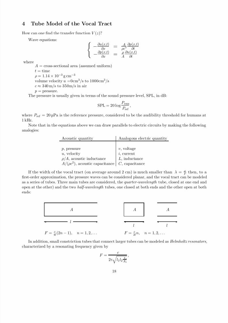
If the width of the vocal tract (on average around 2 cm) is much smaller than λ = cF then, to a
first-order approximation, the pressure waves can be considered planar, and the vocal tract can be modeled
as a series of tubes. Three main tubes are considered, the quarter-wavelength tube, closed at one end and
open at the other) and the two half-wavelength tubes, one closed at both ends and the other open at both
ends:
A
l
F = c4l(2n − 1), n = 1, 2, . . .
A A
l lF = c
2ln, n = 1, 2, . . .
In addition, small constriction tubes that connect larger tubes can be modeled as Helmholtz resonators ,
characterized by a resonating frequency given by
F = c
2π
l1l2A2
A1
,
18

7/18/2019 Course Notes v17
http://slidepdf.com/reader/full/course-notes-v17 19/82
l2
A2
A1
l1
wine bottle.
Figure 10: Helmholtz resonator
where l1 and A1 are the length and cross-sectional area of the constriction, and l2 and A2 are the lengthand area of the previous tube, see Fig. 10.
19
7/18/2019 Course Notes v17
http://slidepdf.com/reader/full/course-notes-v17 20/82
5 Short-Time Speech Analysis
We have previously looked at properties and applications of linear, time-invariant (LTI) systems. However,
when modeling the speech production system as a linear system, it must be considered time-varying due to
the dynamic nature of speech. Thus, in order to correctly analyze the spectral or temporal characteristics
of speech, we can extract short segments that can be assumed stationary. That is, we can window speechsegments wherein information regarding pitch, formants, etc., doesn’t change significantly.
5.1 The Short-Time Fourier Transform
Common tools used to analyze the spectral characteristics of speech with respect to time are the discrete-
time short-time Fourier Transform (STFT) and the discrete STFT. For an input speech signal s (n), the
discrete-time STFT is defined as:
S n
e jω
=∞
m=−∞s (m) w (n − m) e− jωm,
where w (n) is the analysis window used to extract the current speech signal segment, and is nonzeroonly on the range n
∈[0, N w
−1].
The STFT provides information regarding the spectral characteristics of speech signals as a function of
two variables, n and ω . The STFT can be interpreted in two ways:
1. Fixed time (n):If the time index, n, is fixed, the STFT provides the Fourier Transform of xn (m) = s (m) w (n − m),
a speech signal windowed on the range n ∈ [n − N w + 1, n]:
S n
e jω
=∞
m=−∞xn (m) e− jωm.
2. Fixed frequency (ω):
If the frequency, ω , is fixed, S ne jω2 provides the trajectory of energy values with respect to time
contained by the input speech signal at frequency ω .
Note that the discrete-time STFT provides the frequency variable ω as a continuous function, which
may not be feasible for some applications. Thus the discrete STFT can be used:
S n (k) =∞
m=−∞s (m) w (n − m) e− j 2π
N km .
The discrete STFT can also be expressed as the discrete-time STFT, sampled uniformly in the frequency
domain:
S n (k) = S n
e jωω= 2πk
N
5.2 The Analysis Window
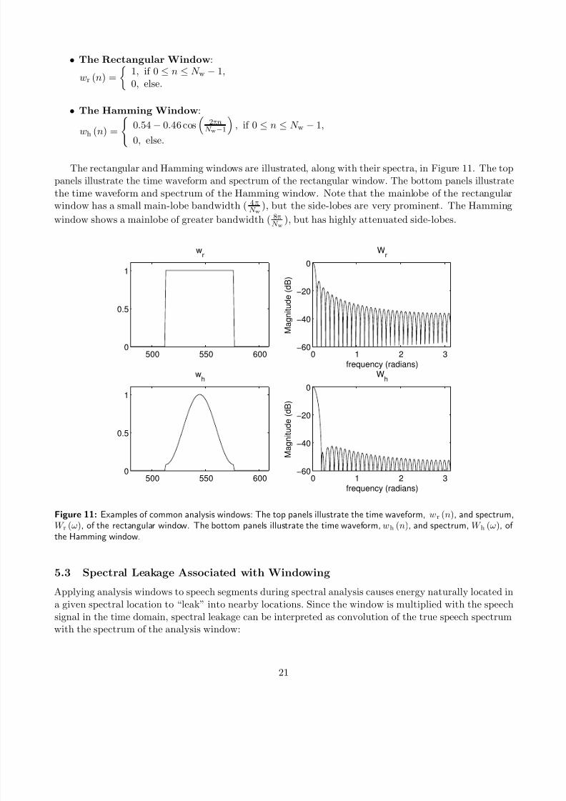
Two common analysis windows used are the rectangular window and the Hamming window:
20
7/18/2019 Course Notes v17
http://slidepdf.com/reader/full/course-notes-v17 21/82
• The Rectangular Window:
wr (n) =
1, if 0 ≤ n ≤ N w − 1,0, else.
• The Hamming Window:
wh (n) = 0.54 − 0.46 cos 2πnN w−1 , if 0 ≤ n ≤ N w − 1,
0, else.
The rectangular and Hamming windows are illustrated, along with their spectra, in Figure 11. The top
panels illustrate the time waveform and spectrum of the rectangular window. The bottom panels illustrate
the time waveform and spectrum of the Hamming window. Note that the mainlobe of the rectangularwindow has a small main-lobe bandwidth ( 4π
N w), but the side-lobes are very prominent. The Hamming
window shows a mainlobe of greater bandwidth ( 8π
N w), but has highly attenuated side-lobes.
500 550 6000
0.5
1
wr
500 550 6000
0.5
1
wh
0 1 2 3−60
−40
−20
0
frequency (radians)
M a g n i t u d e ( d B )
Wr
0 1 2 3−60
−40
−20
0
frequency (radians)
M a g n i t u d e
( d B )
Wh
Figure 11: Examples of common analysis windows: The top panels illustrate the time waveform, wr (n), and spectrum,W r (ω), of the rectangular window. The bottom panels illustrate the time waveform, wh (n), and spectrum, W h (ω), of the Hamming window.
5.3 Spectral Leakage Associated with Windowing
Applying analysis windows to speech segments during spectral analysis causes energy naturally located in
a given spectral location to “leak” into nearby locations. Since the window is multiplied with the speechsignal in the time domain, spectral leakage can be interpreted as convolution of the true speech spectrumwith the spectrum of the analysis window:
21
7/18/2019 Course Notes v17
http://slidepdf.com/reader/full/course-notes-v17 22/82
w (n) s (n) ↔ 1
2πW
e jω ∗ S
e jω
.
Thus, the optimal (yet unrealistic) window would have a frequency response composed of a deltafunction located at ω = 0. Since this window would be infinite in duration, we instead desire to usewindows which have spectra showing low-bandwidth main lobes and highly attenuated side-lobes, andthus approximating the optimal delta function case.
In the case of voiced speech, spectral leakage will cause harmonics to appear as lobes, as opposed toclean spikes.
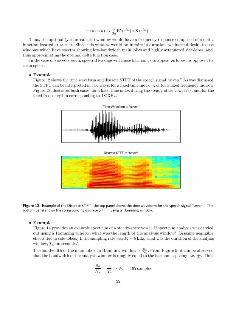
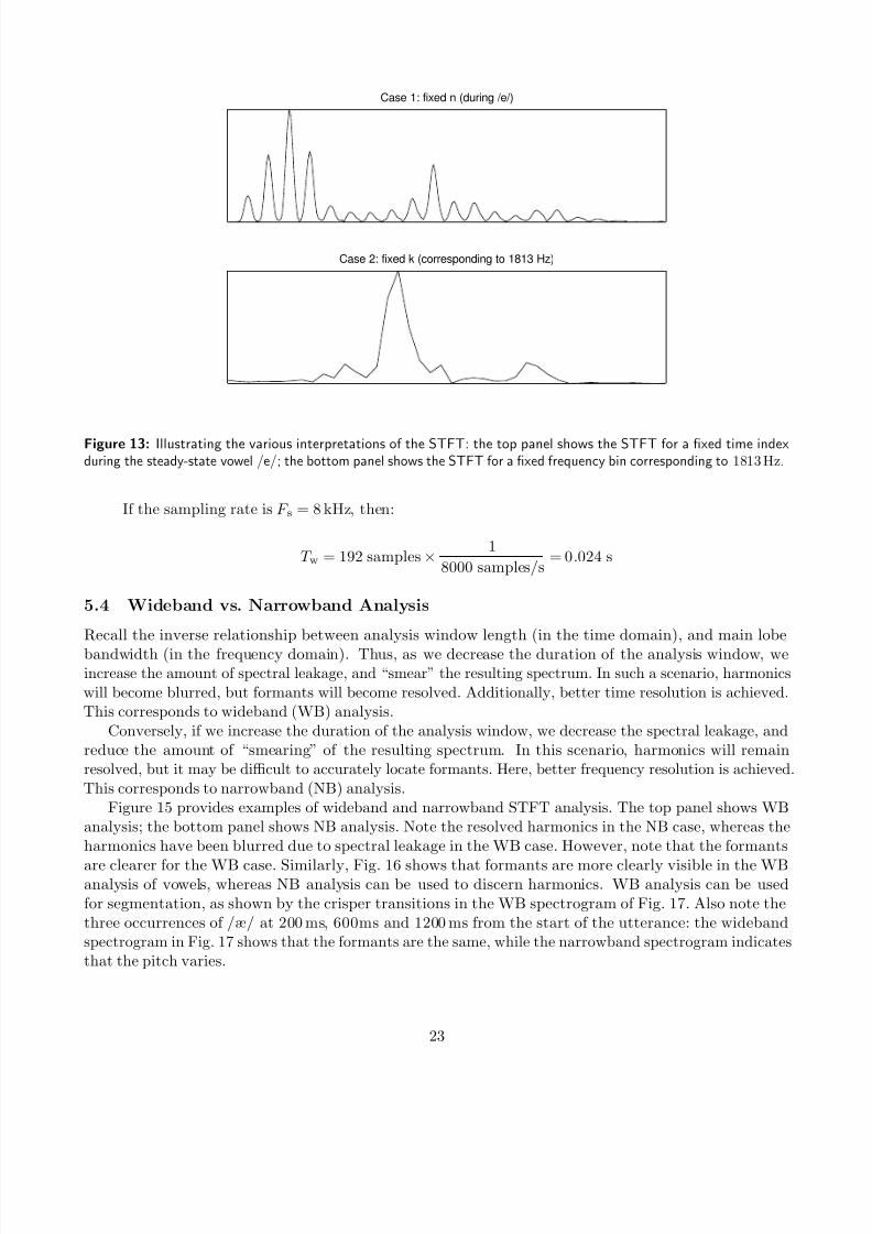
• Example:Figure 12 shows the time waveform and discrete STFT of the speech signal “seven.” As was discussed,
the STFT can be interpreted in two ways, for a fixed time index n, or for a fixed frequency index k.Figure 13 illustrates both cases: for a fixed time index during the steady-state vowel /e/, and for the
fixed frequency bin corresponding to 1813 Hz.
Time Waveform of "seven"
Discrete STFT of "seven"
Figure 12: Example of the Discrete STFT: the top panel shows the time waveform for the speech signal “seven.” Thebottom panel shows the corresponding discrete STFT, using a Hamming window.
• Example:Figure 14 provides an example spectrum of a steady-state vowel. If spectrum analysis was carried
out using a Hamming window, what was the length of the analysis window? (Assume negligibleeffects due to side-lobes.) If the sampling rate was F s = 8 kHz, what was the duration of the analysis
window, T w, in seconds?
The bandwidth of the main lobe of a Hamming window is 8π
N w. From Figure 9, it can be observed
that the bandwidth of the analysis window is roughly equal to the harmonic spacing, i.e. π
24 . Thus:
8π
N w=
π
24 ⇒ N w = 192 samples.
22
7/18/2019 Course Notes v17
http://slidepdf.com/reader/full/course-notes-v17 23/82
Case 1: fixed n (during /e/)
Case 2: fixed k (corresponding to 1813 Hz)
Figure 13: Illustrating the various interpretations of the STFT: the top panel shows the STFT for a fixed time indexduring the steady-state vowel /e/; the bottom panel shows the STFT for a fixed frequency bin corresponding to 1813 Hz.
If the sampling rate is F s = 8 kHz, then:
T w = 192 samples × 1
8000 samples/s = 0.024 s
5.4 Wideband vs. Narrowband Analysis
Recall the inverse relationship between analysis window length (in the time domain), and main lobe
bandwidth (in the frequency domain). Thus, as we decrease the duration of the analysis window, weincrease the amount of spectral leakage, and “smear” the resulting spectrum. In such a scenario, harmonics
will become blurred, but formants will become resolved. Additionally, better time resolution is achieved.
This corresponds to wideband (WB) analysis.Conversely, if we increase the duration of the analysis window, we decrease the spectral leakage, and
reduce the amount of “smearing” of the resulting spectrum. In this scenario, harmonics will remainresolved, but it may be difficult to accurately locate formants. Here, better frequency resolution is achieved.
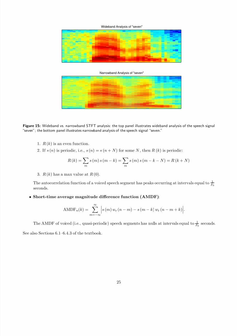
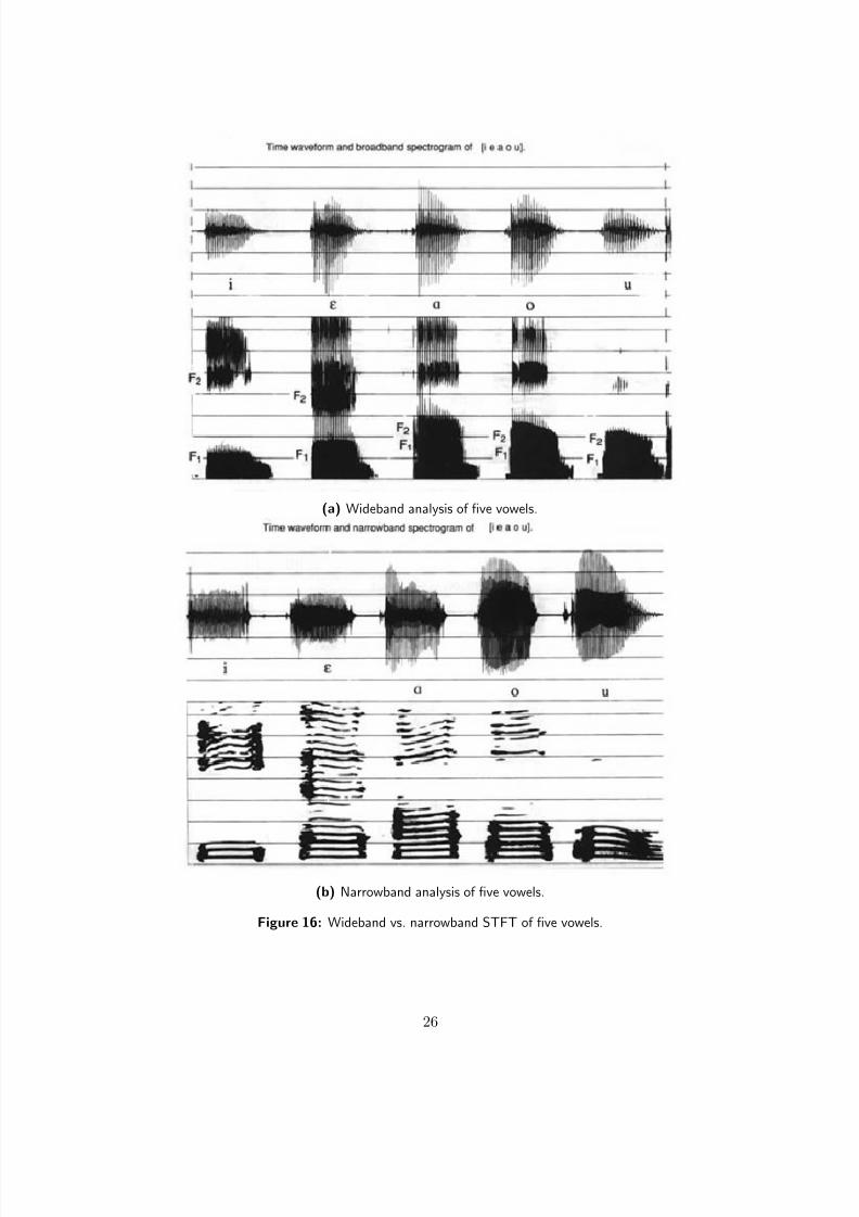
This corresponds to narrowband (NB) analysis.Figure 15 provides examples of wideband and narrowband STFT analysis. The top panel shows WB
analysis; the bottom panel shows NB analysis. Note the resolved harmonics in the NB case, whereas theharmonics have been blurred due to spectral leakage in the WB case. However, note that the formants
are clearer for the WB case. Similarly, Fig. 16 shows that formants are more clearly visible in the WBanalysis of vowels, whereas NB analysis can be used to discern harmonics. WB analysis can be usedfor segmentation, as shown by the crisper transitions in the WB spectrogram of Fig. 17. Also note thethree occurrences of /æ/ at 200 ms, 600ms and 1200 ms from the start of the utterance: the widebandspectrogram in Fig. 17 shows that the formants are the same, while the narrowband spectrogram indicates
that the pitch varies.
23
7/18/2019 Course Notes v17
http://slidepdf.com/reader/full/course-notes-v17 24/82
Figure 14: The spectrum of a steady-state vowel.
5.5 Time-Domain Analysis
Although short-time spectral analysis is widely used for speech processing applications, there exist anumber of short-time time-domain speech features which are also important.
• Short-Time Energy:
STE(n) =∞
m=−∞|s (m)|2 w (n − m) .
The short-time energy is commonly used in voice-activity detection (VAD) and automatic speechrecognition (ASR) of high-energy segments (i.e., vowels). It helps detect pauses, boundaries between
phonemes, words, or syllables, and voiced vs. unvoiced sounds.
• Zero-Crossing Rate:
ZCR(n) =
∞
m=−∞
1
2N w sgn(s (m))
−sgn(s (m
−1))wr (n
−m) .
The zero-crossing rate is used in applications such as VAD to differentiate between periodic signals(low ZCR) and noisy signals (high ZCR). Typical values of ZCRs are 1400 crossings per secondfor voiced sounds and 4900 crossings per second for unvoiced sounds. A threshold at about 2500crossings per second can be used to discriminate voiced vs. unvoiced sounds. ZCR can be used toestimate the frequency of a periodic sound: note that the frequency F a of a sinusoid is related to the
zero crossing rate by
F a = ZCRF s2
.
• Short-Time Autocorrelation:
Rn (k) =∞
m=−∞xn (m) xn (m − k) , (1)
where xn (m) = s (m) w (n − m). The short-time autocorrelation is an important tool in determining
Linear Predictive Coefficients (LPCs), which are used in ASR as well as speech coding.The (non-windowed) autocorrelation function, R (k) =
∞m=−∞ s (m) s (m − k), has several impor-
tant properties:
24
7/18/2019 Course Notes v17
http://slidepdf.com/reader/full/course-notes-v17 25/82
Wideband Analysis of "seven"
Narrowband Analysis of "seven"
Figure 15: Wideband vs. narrowband STFT analysis: the top panel illustrates wideband analysis of the speech signal“seven”; the bottom panel illustrates narrowband analysis of the speech signal “seven.”
1. R (k) is an even function.
2. If s (n) is periodic, i.e., s (n) = s (n + N ) for some N , then R (k) is periodic:
R (k) =m
s (m) s (m − k) =m
s (m) s (m − k − N ) = R (k + N )
3. R (k) has a max value at R (0).
The autocorrelation function of a voiced speech segment has peaks occurring at intervals equal to 1F 0
seconds.
• Short-time average magnitude difference function (AMDF):
AMDFn(k) =
∞m=−∞
s (m) wr (n − m) − s (m − k) wr (n − m + k).
The AMDF of voiced (i.e., quasi-periodic) speech segments has nulls at intervals equal to 1F 0
seconds.
See also Sections 6.1–6.4.3 of the textbook.
25
7/18/2019 Course Notes v17
http://slidepdf.com/reader/full/course-notes-v17 26/82
(a) Wideband analysis of five vowels.
(b) Narrowband analysis of five vowels.
Figure 16: Wideband vs. narrowband STFT of five vowels.
26
7/18/2019 Course Notes v17
http://slidepdf.com/reader/full/course-notes-v17 27/82
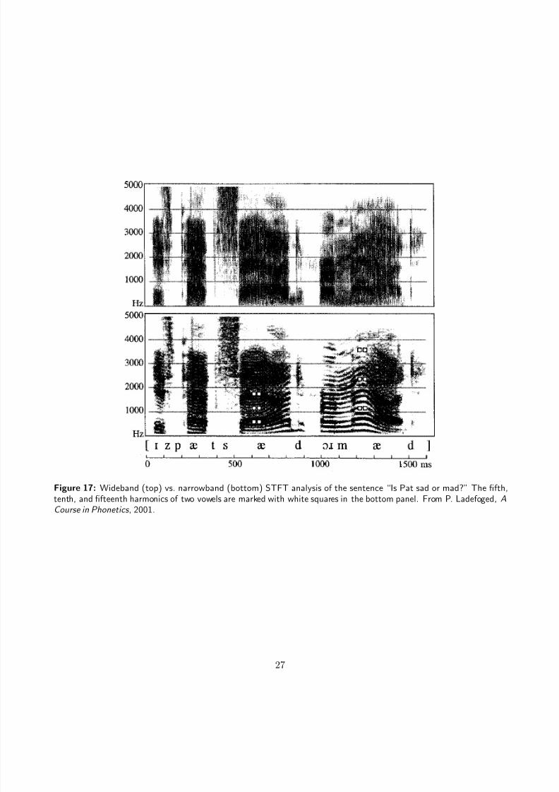
Figure 17: Wideband (top) vs. narrowband (bottom) STFT analysis of the sentence “Is Pat sad or mad?” The fifth,tenth, and fifteenth harmonics of two vowels are marked with white squares in the bottom panel. From P. Ladefoged, ACourse in Phonetics , 2001.
27
7/18/2019 Course Notes v17
http://slidepdf.com/reader/full/course-notes-v17 28/82
6 Linear Prediction Analysis
Linear prediction analysis is based on the notion that speech samples can be predicted accurately fromprevious speech. That is, speech samples can be estimated as a linear combination of past samples. Indetermining the optimal weights by which to combine previous samples, we reveal important spectralinformation regarding the signal.
6.1 The All-Pole Vocal Tract Model
As discussed previously, we assume an all-pole model for the vocal-tract transfer function:
V (z) = G
p1/2k=1
(1 − ckz−1)
1 − c∗kz−1 p2=1
(1 − rz−1)
, p = p1 + p2.
Since speech is naturally a real signal, the poles appear either as complex conjugate pairs, ( ck, c∗k), oras real poles, r. An alternative form of the vocal tract transfer function, which will prove useful for linear
prediction analysis, is:
V (z) = G1 −
pk=1
akz−k. (2)
Recall the expression that relates the source signal U (z) and the output speech S (z) in a linear system:
S (z) = V (z) U (z) . (3)
By substituting the expression for the all-pole transfer function from (2) into the expression for thelinear speech production model (3), we obtain:
S (z) =
p
k=1
akS (z) z−k + GU (z) .
By taking the inverse Z-transform we obtain:
s (n) =
pk=1
aks (n − k) + Gu (n) .
Thus, the current speech sample, s (n) can be predicted as a function of past speech samples{s (n − 1) , . . . , s (n − p)} and the current source signal sample, u (n). The parameters ak are referred to
as the Linear Predictive Coefficients (LPCs).The expression A (z) = 1 − p
k=1 akz−k is referred to as the inverse filter , since it theoretically inverts
the effect of the vocal tract, and returns the source signal. If the vocal tract truly is an all-pole system
and is modeled perfectly during linear predictive analysis, then inverse filtering simply gives the sourcefunction:
A (z) S (z) = A (z) V (z) U (z)
= A (z) G
A (z)U (z)
= GU (z) .
28
7/18/2019 Course Notes v17
http://slidepdf.com/reader/full/course-notes-v17 29/82
6.2 Deriving Linear Predictive Coefficients
To derive the linear predictive coefficients, ak, we first define the least-square error function:
E =∞
n=−∞(s (n) − s (n))2
=∞
n=−∞
s (n) −
pk=1
aks (n − k)2
, (4)
where s (n) is the estimate of s (n) based on the past samples.To derive each optimal coefficient, we minimize the least-square error function by setting the derivative
of E with respect to that coefficient to zero:
∂E
∂ai=
∂
∂ai
∞n=−∞
s (n) −
pk=1
aks (n − k)
2
= 2
∞n=−∞
s (n) − pk=1
aks (n − k) ∂
∂ais (n) −
pk=1
aks (n − k)= −2
∞n=−∞
s (n) s (n − i) −
pk=1
aks (n − k) s (n − i)
= 0.
This leads to the normal equations :
∞n=−∞
s (n) s (n − i) =
pk=1
ak
∞n=−∞
s (n − k) s (n − i) . (5)
Note that using (5) in (4) yields the minimum least-square error:
E min =∞
n=−∞
s2 (n) −
pk=1
aks (n − k) s(n)
. (6)
The minimum error is actually the square of the gain used for the LPC-based vocal tract transferfunction, if the excitation, u (n) is normalized such that
∞n=−∞ u2 (n) = 1.
The normal equations can be solved by means of two methods: using the autocorrelation function or
using the covariance function. The covariance method is more accurate, but induces a higher computational
complexity. There exist efficient algorithms for determining LPCs using the autocorrelation method.
6.3 The Autocorrelation Method
The autocorrelation method for linear prediction analysis assumes that a signal is only nonzero overan interval of N w samples, with N w > p. That is, the signal was windowed prior to analysis. In thefollowing, let us assume that that interval is [0, N w − 1], and, in the notation of (1), let R (k) = Rn (k),with n = N w − 1. When applying the autocorrelation function:
R (i) =
N w−1m=i
x (m) x (m − i) , i = 0, . . . , N w − 1,
29
7/18/2019 Course Notes v17
http://slidepdf.com/reader/full/course-notes-v17 30/82
where x (m) = s (m) w (n − m), n = N w − 1. Because x(m) is non-zero only for m ∈ [0, N w − 1], andx(m − i) is non-zero for m ∈ [i, N w + i − 1], the summation only needs to be carried out over the range[i, N w − 1]. In this case, the normal equations (5), where we use the windowed signal, x (n), instead of s (n), become:
R (i) =
p
k=1 akR (i − k) , and more generally
R (i) =
pk=1
akR (|i − k|) , i = 1, . . . , p .
Note that in the above equation we took advantage of the property that the autocorrelation is an even
function. The normal equations (5) can be written in matrix form as:
R (0) R (1) · · · R ( p − 1)R (1) R (0) · · ·
... ...
. . .
R ( p − 1) R (0)
R
a1...
a p
a
=
R (1)
...
R ( p)
r
.
The matrix R is Toeplitz, meaning that is symmetric with identical elements on the diagonals. Thereexist efficient algorithms to invert Toeplitz matrices, so the matrix a can be determined as:
a = R −1r.
The minimum least-square error (6) is then calculated as:
E min = R (0) − p
k=1
akR (k) .
• Example: Consider the speech segment [3, 2, −1, 1] (note that we used N w = 4). Find the 2nd-order
vocal tract transfer function using linear predictive analysis.
R (i) = [15, 3, −1, 3].
For order p = 2:
R =
15 33 15
, r =
3−1
, a = R −1r =
2
9− 1
9
,
E min = R (0) −2
k=1
akR (k)
= 15 −
2
9
(3) −
−1
9
(−1) =
128
9 ≈ 14.22,
G =
E min ≈ 3.77,
⇒ V (z) = 3.77
1 − 29 z−1 + 1
9 z−2,
30
7/18/2019 Course Notes v17
http://slidepdf.com/reader/full/course-notes-v17 31/82
with roots at z = c1 and z = c∗1, with c1 =
1 + j√
8
/9 ≈ 0.11 + j0.31. This corresponds to anestimated formant F 1 ≈ 0.196F s.
The choice of the order p during LPC analysis should reflect the number of formants expected. Recall
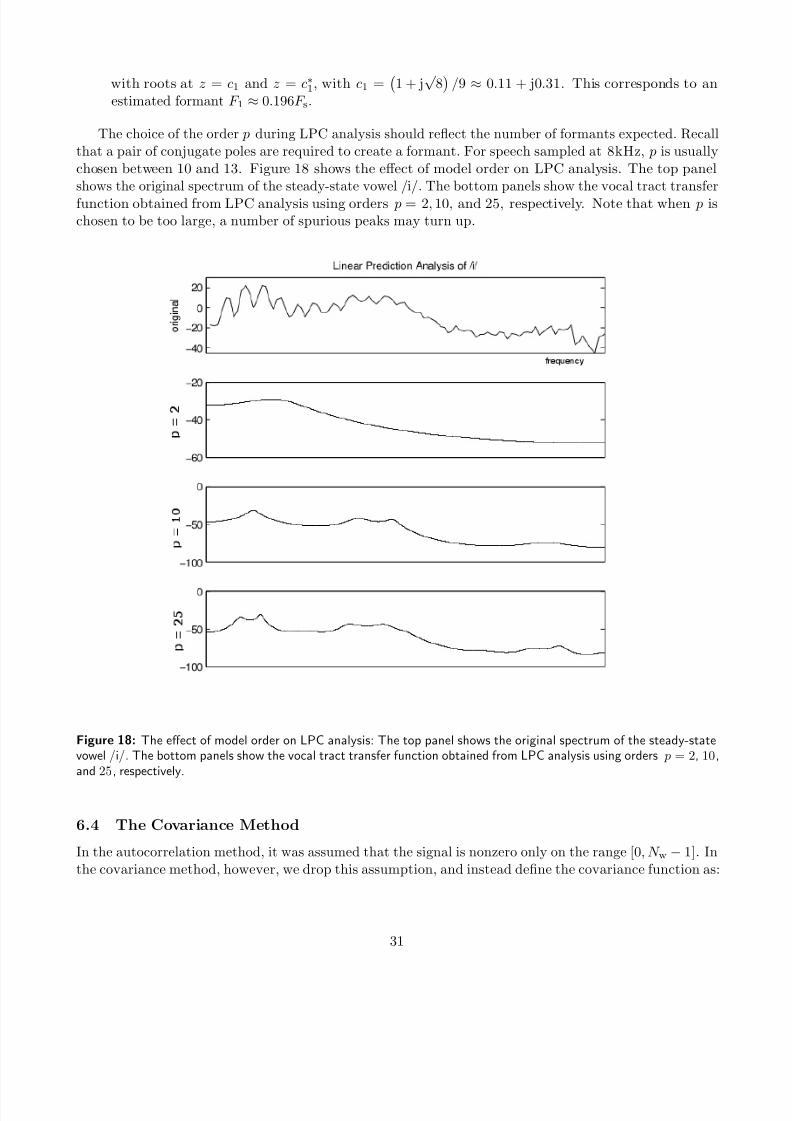
that a pair of conjugate poles are required to create a formant. For speech sampled at 8kHz, p is usuallychosen between 10 and 13. Figure 18 shows the effect of model order on LPC analysis. The top panelshows the original spectrum of the steady-state vowel /i/. The bottom panels show the vocal tract transfer
function obtained from LPC analysis using orders p = 2, 10, and 25, respectively. Note that when p ischosen to be too large, a number of spurious peaks may turn up.
Figure 18: The effect of model order on LPC analysis: The top panel shows the original spectrum of the steady-statevowel /i/. The bottom panels show the vocal tract transfer function obtained from LPC analysis using orders p = 2, 10,and 25, respectively.
6.4 The Covariance Method
In the autocorrelation method, it was assumed that the signal is nonzero only on the range [0, N w − 1]. In
the covariance method, however, we drop this assumption, and instead define the covariance function as:
31
7/18/2019 Course Notes v17
http://slidepdf.com/reader/full/course-notes-v17 32/82
φ (i, k) =
pn=0
s (n − k) s (n − i) , 0 ≤ i ≤ p, 0 ≤ k ≤ p. (7)
Note that since the signal is not “windowed,” as in the autocorrelation case, the summation in (7) isalways carried out on the range [0, p].
The normal equations for the covariance method become:
φ (i, 0) =
pk=1
akφ (i, k) , for 1 ≤ i ≤ p.
In matrix form, the normal equations can be expressed as:
φ (1, 1) φ (1, 2) · · · φ (1, p)φ (2, 1) φ (2, 2) · · ·
... ...
. . .
φ ( p, 1) φ ( p, p)
Φ
a1
...a p
a
=
φ (1, 0)
...φ ( p, 0)
φ
.
Note that the matrix Φ is symmetric but not necessarily Toeplitz. Thus it is generally more difficultto determine the inverse of Φ than of R . Nevertheless, the linear predictive coefficients can be solved as:
a = Φ−1φ.
Furthermore, the minimum error is determined as:
E min = φ (0, 0) − pk=1
akφ (0, k) .
The covariance matrix can be interpreted as the error (4) being windowed, as opposed to the signalbeing windowed (as in the autocorrelation case).
• Example: Consider the speech segment [. . . , −3, 1, −2, 3, 2, −1, 1, −2, 0, 1, . . . ] (compare this withthe previous example). Find the 2nd-order vocal tract transfer function using the covariance method
of linear predictive analysis. The origin is denoted by the underscore.For order p = 2:
Φ =
17 −2−2 14
, φ =
−2−4
, a = Φ−1φ = − 1
117
1836
,
E min = φ (0, 0) −2
k=1
akφ (0, k)
= 14 −− 18
117 (−2) −− 36
117 (−4) =
1458
117 ≈ 12.46,
G =
E min ≈ 3.53,
⇒ V (z) = 3.68
1 + 18117 z−1 + 36
117 z−2,
with poles at z = c1 and z = c∗1, with c1 = 1117
−9 + j√
4131 ≈ −0.077+j0.55, corresponding to an
estimated formantF 1 ≈ 0.272F s.
32
7/18/2019 Course Notes v17
http://slidepdf.com/reader/full/course-notes-v17 33/82
Part II
Image Processing
7 Examples of Applications
• Photography
• Computer vision
• Remote sensing
– Planetary exploration
– Environmental monitoring
– Geology
– Reconnaisance
• Medicine
– Magnetic resonance imaging (MRI)
– Positron emission tomography (PET)
– Angiograms
– Digital radiography
• Communications
– Videoconferencing
– HDTV
• Chemistry
• Etc.
8 Image Processing v. 1D DSP
• Similarities
– Sampling
– Filtering
– Impulse response
– Transforms
• Differences
– Data size
– Complexity (1D vs. 2D)
– Conceptual challenges due to dimensionality
– Interface with human visual system
33

7/18/2019 Course Notes v17
http://slidepdf.com/reader/full/course-notes-v17 34/82
9 Overview
• Introduction
• 2D linear system theory
– Math preliminaries
– Continuous 2D systems, including convolution, FT– Discrete systems
– Image sampling
• Image transforms
– Fourier (2D discrete)
– Discrete cosine transform (DCT)
– Other (KL, etc.)
• Image Enhancement
– Histogram modification
– Edge detection
– Noise filtering
• Image compression
• Human visual perception vs. digital image processing
34
7/18/2019 Course Notes v17
http://slidepdf.com/reader/full/course-notes-v17 35/82
10 1D vs. 2D
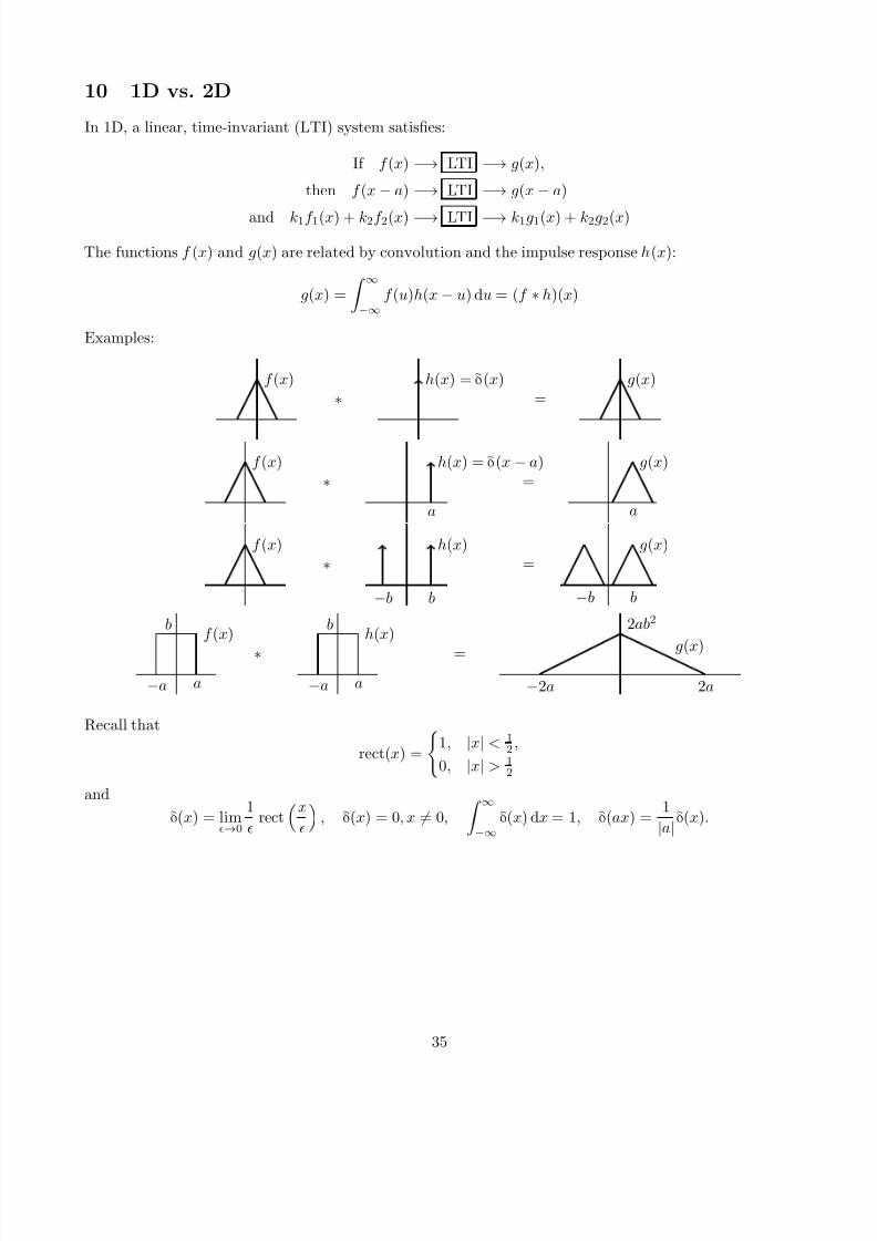
In 1D, a linear, time-invariant (LTI) system satisfies:
If f (x) −→ LTI −→ g(x),
then f (x − a) −→ LTI −→ g(x − a)
and k1f 1(x) + k2f 2(x) −→ LTI −→ k1g1(x) + k2g2(x)
The functions f (x) and g(x) are related by convolution and the impulse response h(x):
g(x) =
∞−∞
f (u)h(x − u) du = (f ∗ h)(x)
Examples:
f (x)
∗h(x) = δ(x)
=g(x)
f (x)
∗a
h(x) = δ(x − a)=
g(x)
a
f (x)
∗
b
h(x)
−b
=g(x)
b−b
−a a
f (x)b
∗−a a
h(x)b
=
−2a
2ab2
2a
g(x)
Recall that
rect(x) =
1, |x| < 1
2 ,
0, |x| > 12
and
δ(x) = lim→0
1
rect
x
, δ(x) = 0, x = 0,
∞−∞
δ(x) dx = 1, δ(ax) = 1
|a|δ(x).
35

7/18/2019 Course Notes v17
http://slidepdf.com/reader/full/course-notes-v17 36/82
The 2D impulse is defined
δ(x, y) = lim→0
1
rect
x
1
rect
y
= δ(x)δ(y),
δ(x, y) = 0, for (x, y) = (0, 0), and
δ(x, y) dx dy = 1.
Note thatf (x, y) ∗ δ(x − a, y − b) = f (x − a, y − b).
x
y
δ(x, y)
x
y
δ(x − a, y − b)
ba
A 2D linear, shift-invariant (LSI) system satisfies:
If f (x, y) −→ LSI −→ g(x, y),
then f (x − a, y − b) −→ LSI −→ g(x − a, y − b)
and k1f 1(x, y) + k2f 2(x, y) −→ LSI −→ k1g1(x, y) + k2g2(x, y)
An LSI system can be completely defined by its impulse response:
δ(x, y) −→ LSI −→ h(x, y)
Example: Astronomical imaging: Actual image of a star resembles a δ(x − a, y − b) and the resultingimage is h(x − a, y − b). Several stars produce similar images.
In general, the output of a 2D LSI system can be understood as the superposition of shifted and scaled
versions of h(x, y):
g(x, y) =
f (x, y)h(x − x, y − y) dx dy = (f ∗ h)(x, y) = (h ∗ f )(x, y).
Examples (note: a dot represents a delta)
x
y
δ(x − a, y)
a
f (x, y)
x
y
δ(x − b, y)
b
h(x, y)
x
y
δ(x − a − b, y)
a + b
g(x, y)
x
y
a−d
c
−c
f (x, y)
x
y
b
h(x, y)
x
y
b − d
a + b
c
−c
g(x, y)
36
7/18/2019 Course Notes v17
http://slidepdf.com/reader/full/course-notes-v17 37/82
11 The Fourier Transform
The FT is probably the single most important mathematical tool in image processing. We will review the
1D FT and then study the 2D FT.Although image processing generally involves 2D discrete functions, it uses many techniques modeled
on analog processes. A good understanding of 1D and 2D continuous FT theory is essential to imageprocessing.
Given a 1D continuous function f (x), the FT and invest FT (IFT) are defined as follows
F (u) :=
∞−∞
f (x)e− j2πux dx = F[f ](u)
f (x) :=
∞−∞
F (u)e j2πux du = F−1[F ](x).
(8a)
(8b)
The units of u are the inverse of the units of x, i.e., if x is measured in seconds, then u is measured inhertz, if x is in meters, u is in cycles per meter (spacial frequency).
F (u) is a decomposition of f (x) into its component frequencies.Example:
F (u) = 12δ(u + a) + 12δ(u − a).
Using the sifting property of the delta function: ∞−∞
δ(x − x0)f (x) d(x) = f (x0),
we obtain
f (x) =
∞−∞
1
2δ(u + a) +
1
2δ(u − a)
e j2πux dx =
1
2e j2πax +
1
2e− j2πax = cos(2πax).
In general, the 1D FT provides the decomposition of f (x) in terms of cosines of the form A cos(2πf x + θ).
The set of all cosines at all combinations of A, f , and θ, provides a complete basis to build 1D functions.Some important transforms:
δ(x) −→ 1
b rectx
a
−→ b|a| sinc(au)
e−πx2 −→ e−πu2 ,
where
sinc(x) := sin(πx)
πx
is the normalized cardinal sine function.
The Convolution Theorem states that if
g(x) = (f ∗ h)(x) =
∞−∞
f (z)h(x − z) dz =
∞−∞
h(z)f (x − z) dz,
thenG(u) = F (u)H (u),
where G(u), F (u), and H (u) are the FTs of g(x), f (x), and h(x), respectively.
37
7/18/2019 Course Notes v17
http://slidepdf.com/reader/full/course-notes-v17 38/82
The 2D FT of f (x, y) expresses f (x, y) as a sum of 2D sinusoids A cos(ax + by + θ). Each sinusoidhas spatial frequency ρ =
√ a2 + b2, period 1/ρ, and its contours of constant amplitude make an angle
φ = tan−1 ba with respect to the x-axis.
Given a 2D continuous function f (x, y)
F (u, v) := f (x, y)e− j2π(ux+vy) dx dy = F[f ](u, v)
f (x, y) :=
F (u, v)e j2π(ux+vy) du dv = F−1[F ](x, y).
(9a)
(9b)
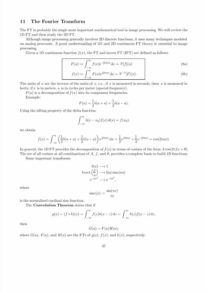
The 2D FT expresses f (x, y) in terms of a combination of 2D sinusoidal corrugations .Example:
F (u, v) = 1
2δ(u + a, v) +
1
2δ(u − a, v)
u
vF (u, v)
−a a
f (x, y) = cos(2πax).
In this case, f (x, y) depends only on x and the corrugations are parallel with the y-axis.
x
y
u
v
−a a
A rotation of f (x, y) causes a corresponding rotation of F (u, v)
x
y
tan−1 b
a
u
v
−aa
tan−1 ba
38
7/18/2019 Course Notes v17
http://slidepdf.com/reader/full/course-notes-v17 39/82
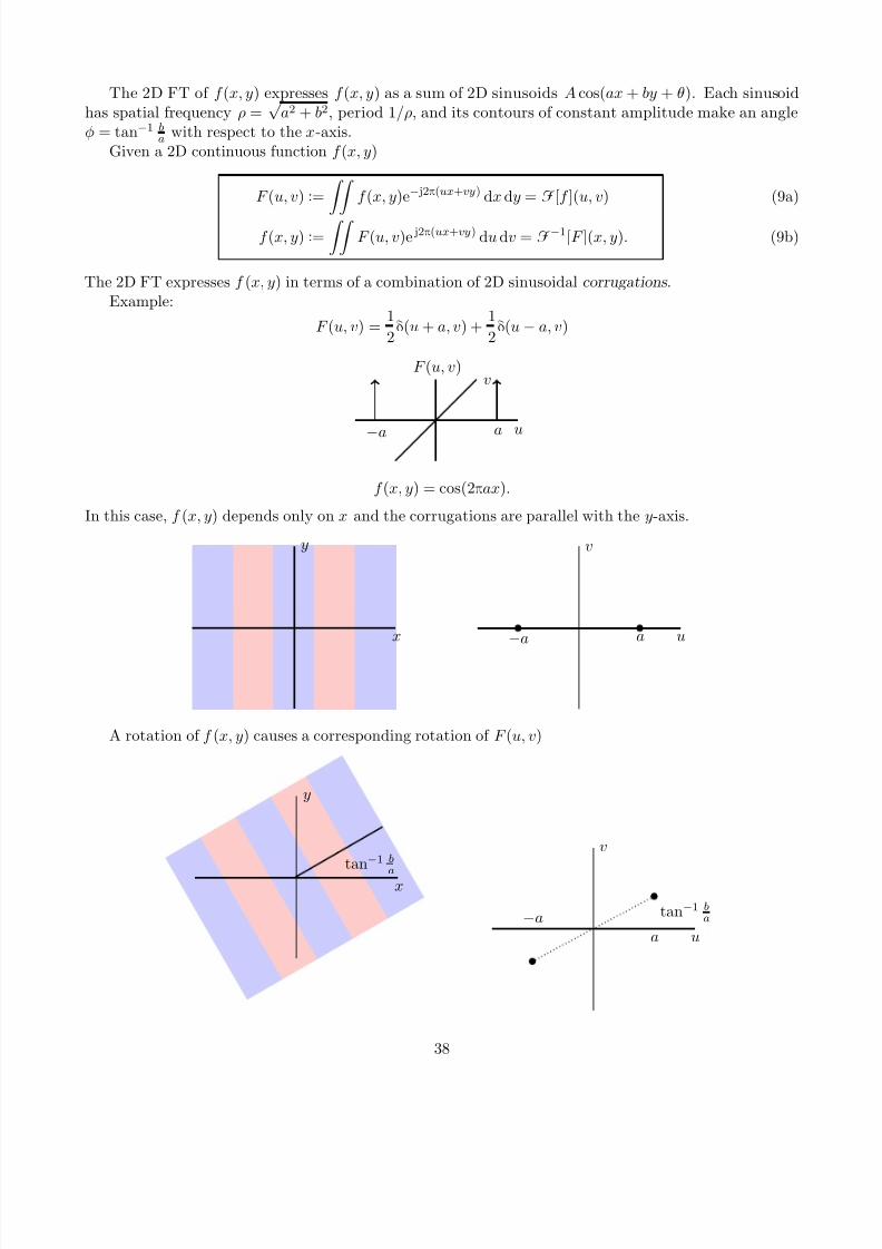
Figure 19: Illustration of the Fourier transform of a sinusoidal corrugation.
The set of all sinusoidal corrugations (at all amplitudes, frequencies, phase shifts, and rotations)constitutes a complete basis for any function f (x, y). The 2D FT expresses f (x, y) as a linear combination
of such corrugations.Theorems for the 2D FT are generally analogous to their 1D counterparts
39

7/18/2019 Course Notes v17
http://slidepdf.com/reader/full/course-notes-v17 40/82
1D: f (x) ↔ F (u) 2D: f (x, y) ↔ F (u, v)
Shift f (x − a) ↔ e− j2πauF (u) f (x − a, y − b) ↔ e− j2π(au+bv)F (u, v)Stretch f (ax) ↔ 1
|a|F ua
f (ax, by) ↔ 1
|ab|F ua , vb
Convolution (f ∗ g)(x) ↔ F (u)G(u) (f ∗ g)(x, y) ↔ F (u, v)G(u, v)Correlation rfg(x) = f (x) ∗ g∗(−x) ↔ F (u)G∗(u) rfg(x, y) = f (x, y) ∗ g∗(−x, −y) ↔ F (u, v)G∗(u, v)
f ∗(x) ↔ F ∗(−u) f ∗(x, y) ↔ F ∗(−u, −v)
f (−x) ↔ F (−u) f (−x, −y) ↔ F (−u, −v)f ∗(−x) ↔ F ∗(u) f ∗(−x, −y) ↔ F ∗(u, v)
The cross-correlation between f and g is defined as
rfg(x) :=
∞−∞
f (u)g∗(u − x) du.
Note from the table above thatF[rfg](u, v) = (F[rgf ](u, v))∗ ,
which shows, upon IFT, thatrgf (x, y) = r∗fg(−x, −y).
40
7/18/2019 Course Notes v17
http://slidepdf.com/reader/full/course-notes-v17 41/82
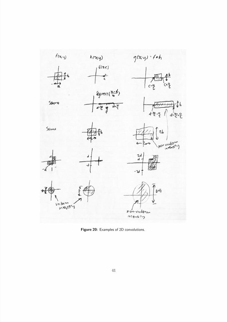
Figure 20: Examples of 2D convolutions.
41
7/18/2019 Course Notes v17
http://slidepdf.com/reader/full/course-notes-v17 42/82
11.1 FT of Separable Functions
If f (x, y) = f 1(x)f 2(y) then the FT can be written
F (u, v) =
f 1(x)e− j2πux f 2(y)e− j2πvy dx dy = F 1(u)F 2(v),
where F 1(u) = F[f 1](u) and F 2(v) = F[f 2](v). Therefore, if f (x, y) is separable, so is F (u, v).
Example:
f (x, y) =
1, |x| < W x
2 and |y| < W y
2 ,
0, elsewhere.
Using the rect(·) function
rect(x) =
1, |x| < 1
2 ,
0, elsewhere,
we have that
f (x, y) = rect
x
W x
rect
y
W y
.
We also know that
F
rect
x
W x
(u) = W x sinc(W xu),
F
rect
y
W y
(v) = W y sinc(W yv).
ThereforeF (u, v) = W x W y sinc(W xu)sinc(W yv).
12 Discrete Signals
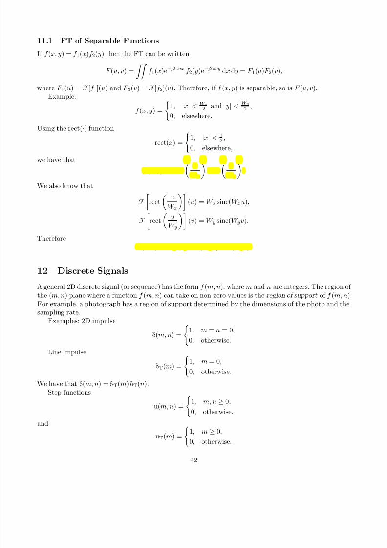
A general 2D discrete signal (or sequence) has the form f (m, n), where m and n are integers. The region of the (m, n) plane where a function f (m, n) can take on non-zero values is the region of support of f (m, n).
For example, a photograph has a region of support determined by the dimensions of the photo and thesampling rate.
Examples: 2D impulse
δ(m, n) =
1, m = n = 0,
0, otherwise.
Line impulse
δT(m) =
1, m = 0,
0, otherwise.
We have that δ(m, n) = δT(m) δT(n).Step functions
u(m, n) =
1, m, n ≥ 0,
0, otherwise.
and
uT(m) =
1, m ≥ 0,
0, otherwise.
42
7/18/2019 Course Notes v17
http://slidepdf.com/reader/full/course-notes-v17 43/82
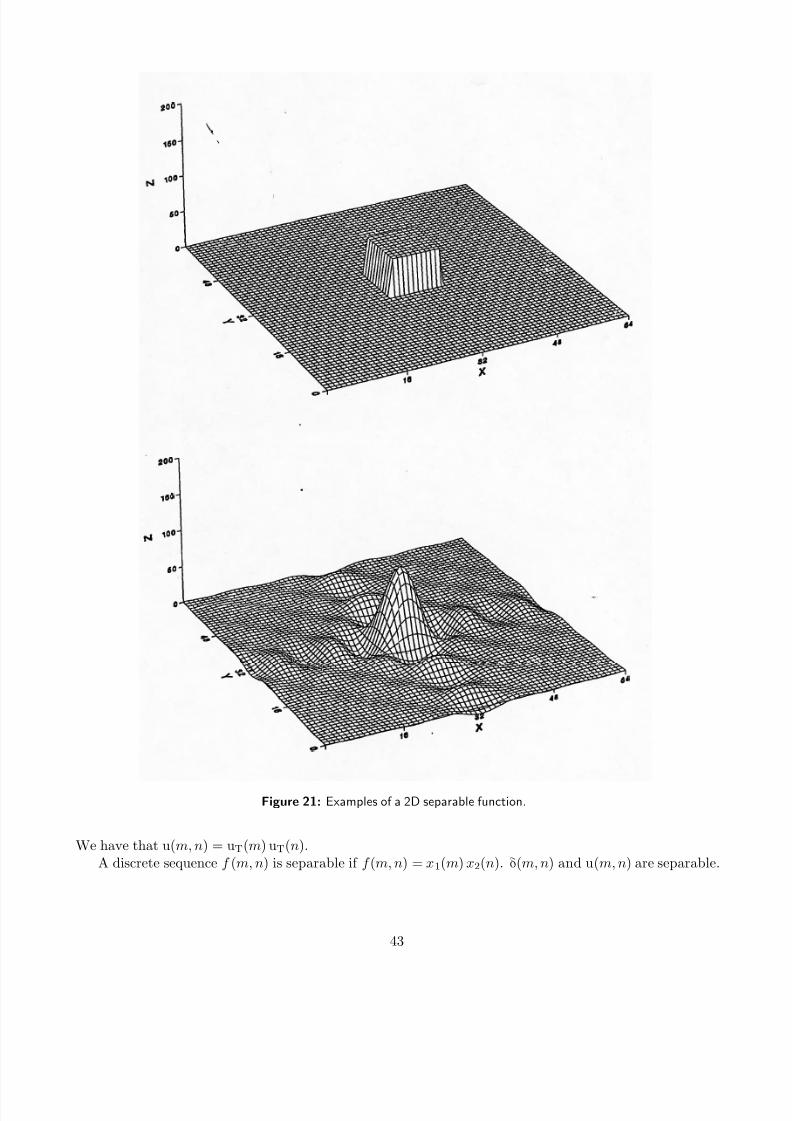
Figure 21: Examples of a 2D separable function.
We have that u(m, n) = uT(m) uT(n).A discrete sequence f (m, n) is separable if f (m, n) = x1(m) x2(n). δ(m, n) and u(m, n) are separable.
43
7/18/2019 Course Notes v17
http://slidepdf.com/reader/full/course-notes-v17 44/82
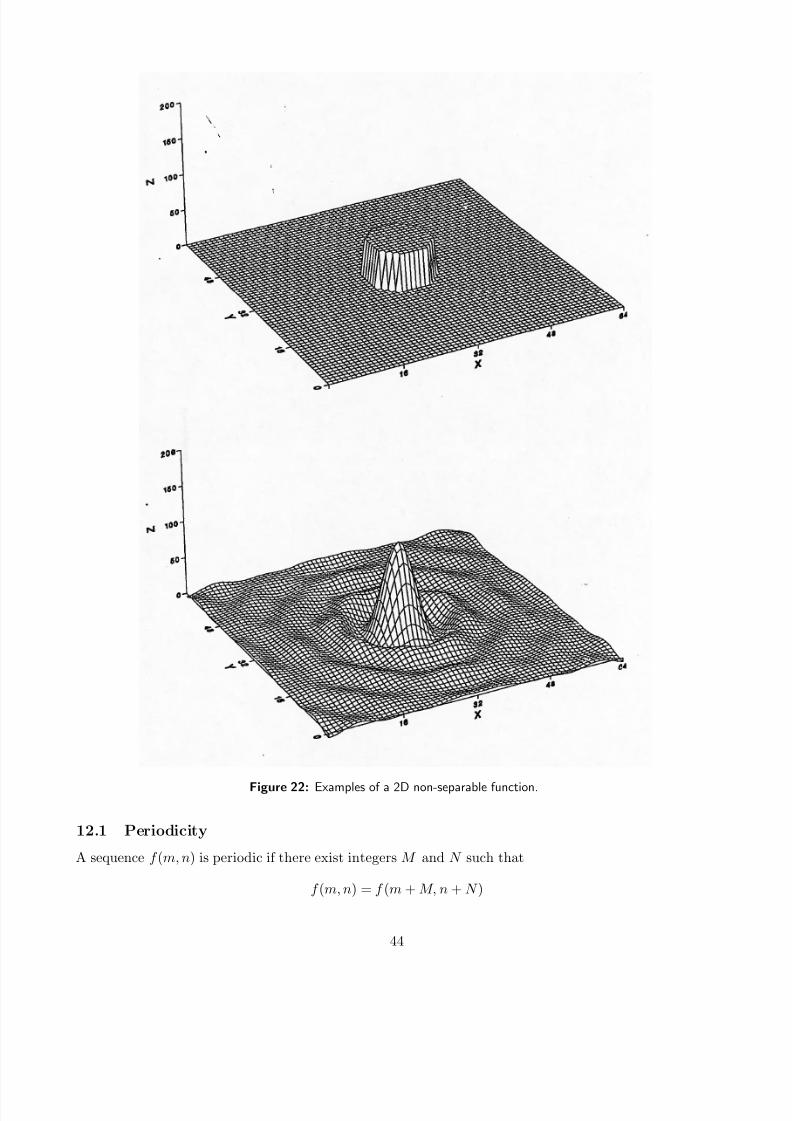
Figure 22: Examples of a 2D non-separable function.
12.1 Periodicity
A sequence f (m, n) is periodic if there exist integers M and N such that
f (m, n) = f (m + M, n + N )
44
7/18/2019 Course Notes v17
http://slidepdf.com/reader/full/course-notes-v17 45/82
for all m, n.
12.2 Input-Output
A 2D system produces an output sequence g(m, n) from an input sequence f (m, n):
g(m, n) = T [f (m, n)] .
Linearity:T [k1f 1(m, n) + k2f 2(m, n)] = k1g1(m, n) + k2g2(m, n).
Shift-invariance:
If T [f (m, n)] = g(m, n), then T [f (m − m1, n − n1)] = g(m − m1, n − n1).
The response h(m, n) of a 2D LSI system to the input δ(m, n) is the impulse response. The function|h(m, n)|2 is sometimes called point spread function.
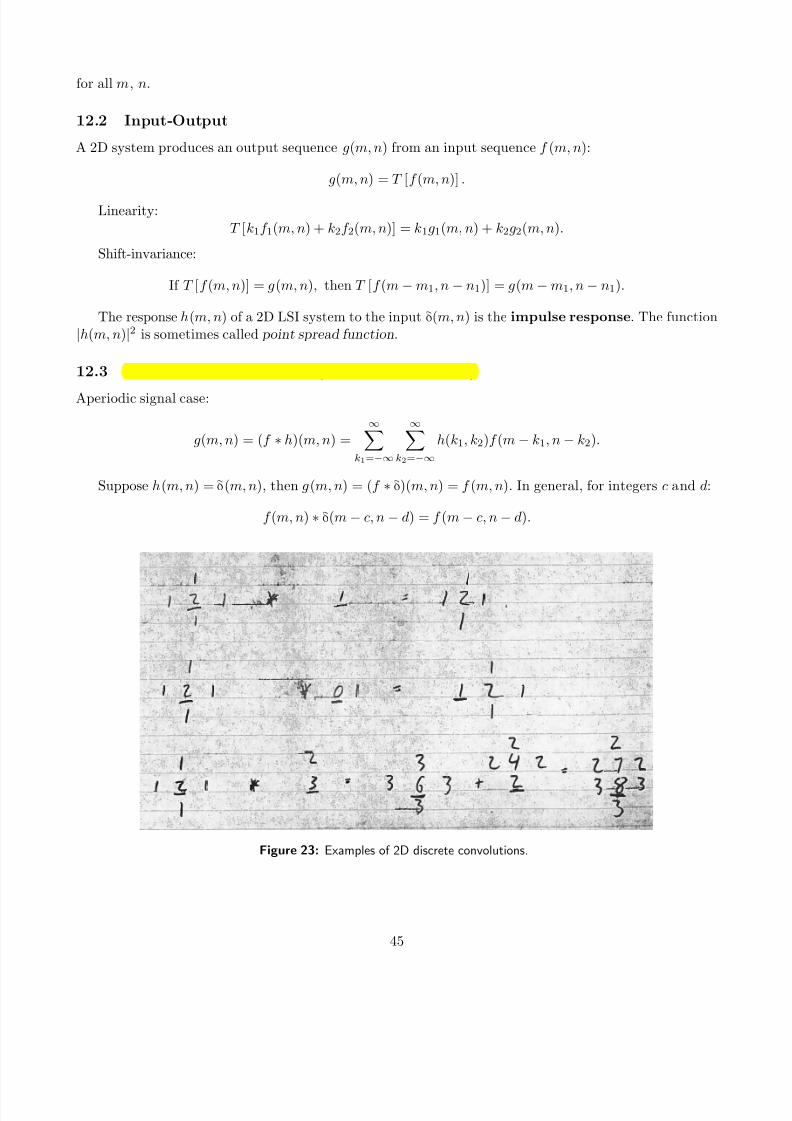
12.3 2D Discrete Convolution (Linear Convolution)
Aperiodic signal case:
g(m, n) = (f ∗ h)(m, n) =∞
k1=−∞
∞k2=−∞
h(k1, k2)f (m − k1, n − k2).
Suppose h(m, n) = δ(m, n), then g(m, n) = (f ∗ δ)(m, n) = f (m, n). In general, for integers c and d:
f (m, n) ∗ δ(m − c, n − d) = f (m − c, n − d).
Figure 23: Examples of 2D discrete convolutions.
45

7/18/2019 Course Notes v17
http://slidepdf.com/reader/full/course-notes-v17 46/82
A general sequence f (m, n) can be expressed as a sum of weighted, shifted impulses:
f (m, n) = f (0, 0)δ(m, n) + f (1, 0)δ(m − 1, n) + f (0, 1)δ(m, n − 1) + · · ·
=
∞k1=−∞
∞k2−=−∞
f (k1, k2)δ(m − k1, n − k2).
Therefore the output of an LSI system can be written as
g(m, n) = f (0, 0)h(m, n) + f (1, 0)h(m − 1, n) + f (0, 1)h(m, n − 1) + · · ·
=∞
k1=−∞
∞k2−=−∞
f (k1, k2)h(m − k1, n − k2) = (f ∗ h)(m, n).
As with 1D, 2D convolution is commutative, associative, and distributive.An LSI system is separable if h(m, n) is separable. A separable system’s response can be computed
with 1D convolutions and requires fewer multiplications to calculate.An LSI system is stable if every bounded input produces a bounded output
12.4 Cross-correlation
For aperiodic signals
rfg(m, n) :=∞
k1=−∞
∞k2=−∞
f (k1, k2)g∗(k1 − m, k2 − n) = f (m, n) ∗ g∗(−m, −n).
Figure 24: Examples of 2D discrete cross-correlations.
12.5 2D DTFT
For a stable aperiodic sequence with
∞m=−∞
∞n=−∞
|u(m, n)| < ∞,
46
7/18/2019 Course Notes v17
http://slidepdf.com/reader/full/course-notes-v17 47/82
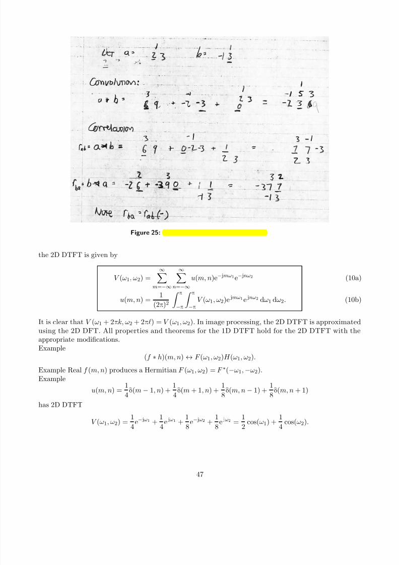
Figure 25: 2D convolutions vs. cross-correlations.
the 2D DTFT is given by
V (ω1, ω2) =∞
m=−∞
∞n=−∞
u(m, n)e− jmω1e− jnω2
u(m, n) = 1(2π)2
π−π
π−π
V (ω1, ω2)e jmω1e jnω2 dω1 dω2.
(10a)
(10b)
It is clear that V (ω1 + 2πk, ω2 + 2π) = V (ω1, ω2). In image processing, the 2D DTFT is approximatedusing the 2D DFT. All properties and theorems for the 1D DTFT hold for the 2D DTFT with theappropriate modifications.Example
(f ∗ h)(m, n) ↔ F (ω1, ω2)H (ω1, ω2).
Example Real f (m, n) produces a Hermitian F (ω1, ω2) = F ∗(−ω1, −ω2).Example
u(m, n) = 1
4
δ(m
−1, n) +
1
4
δ(m + 1, n) + 1
8
δ(m, n
−1) +
1
8
δ(m, n + 1)
has 2D DTFT
V (ω1, ω2) = 1
4e− jω1 +
1
4e jω1 +
1
8e− jω2 +
1
8e jω2 =
1
2 cos(ω1) +
1
4 cos(ω2).
47
7/18/2019 Course Notes v17
http://slidepdf.com/reader/full/course-notes-v17 48/82
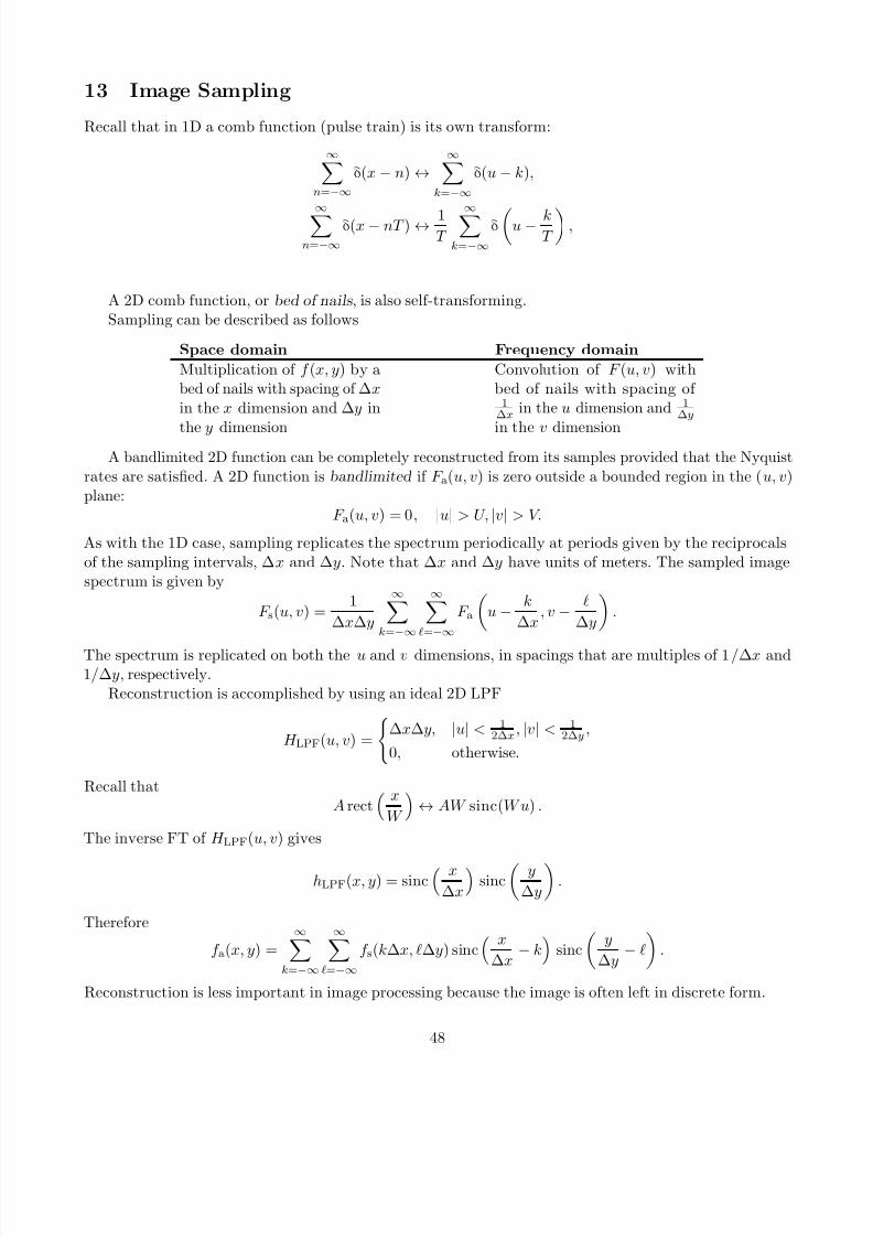
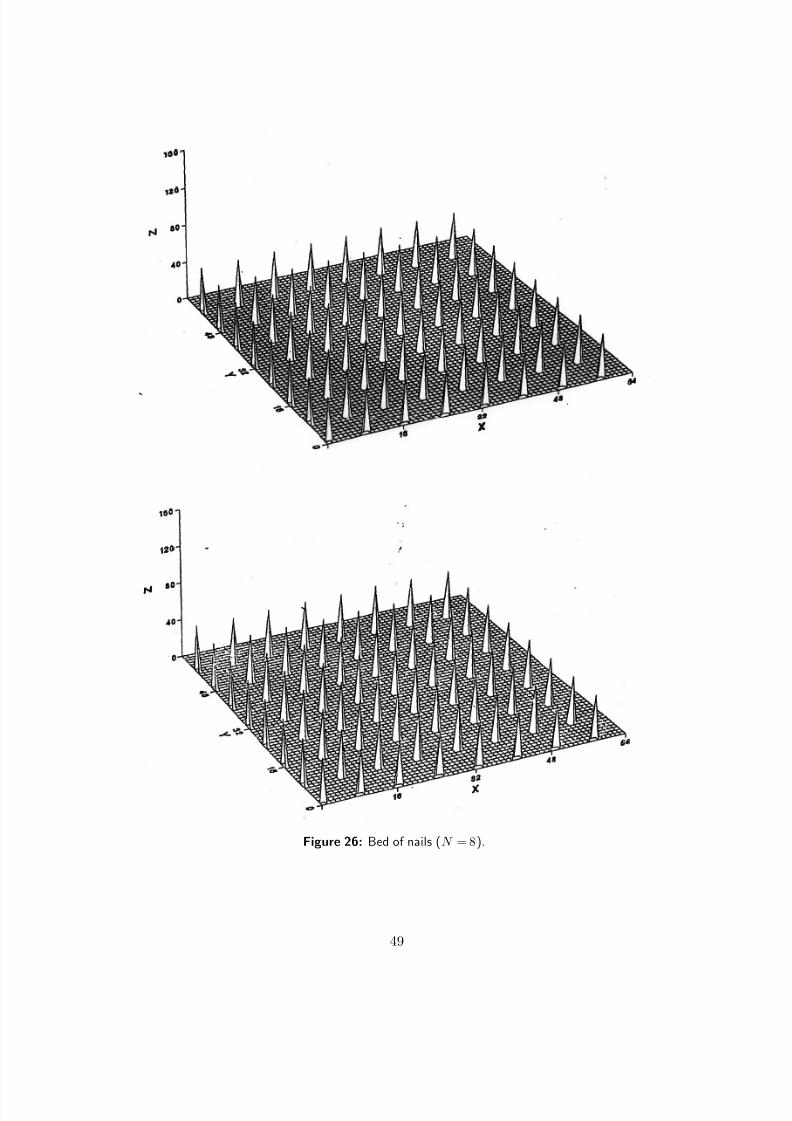
13 Image Sampling
Recall that in 1D a comb function (pulse train) is its own transform:
∞n=−∞
δ(x − n) ↔∞
k=−∞δ(u − k),
∞n=−∞
δ(x − nT ) ↔ 1T
∞k=−∞
δ
u − kT
,
A 2D comb function, or bed of nails , is also self-transforming.Sampling can be described as follows
Space domain Frequency domain
Multiplication of f (x, y) by abed of nails with spacing of ∆xin the x dimension and ∆y in
the y dimension
Convolution of F (u, v) withbed of nails with spacing of
1∆x in the u dimension and 1
∆y
in the v dimensionA bandlimited 2D function can be completely reconstructed from its samples provided that the Nyquist
rates are satisfied. A 2D function is bandlimited if F a(u, v) is zero outside a bounded region in the (u, v)plane:
F a(u, v) = 0, |u| > U, |v| > V.
As with the 1D case, sampling replicates the spectrum periodically at periods given by the reciprocalsof the sampling intervals, ∆x and ∆y. Note that ∆x and ∆y have units of meters. The sampled imagespectrum is given by
F s(u, v) = 1
∆x∆y
∞k=−∞
∞=−∞
F a
u − k
∆x, v −
∆y
.
The spectrum is replicated on both the u and v dimensions, in spacings that are multiples of 1/∆x and1/∆y, respectively.
Reconstruction is accomplished by using an ideal 2D LPF
H LPF(u, v) =
∆x∆y, |u| < 1
2∆x , |v| < 12∆y ,
0, otherwise.
Recall thatA rect
x
W
↔ AW sinc(W u) .
The inverse FT of H LPF(u, v) gives
hLPF(x, y) = sinc x
∆x
sinc
y∆y
.
Therefore
f a(x, y) =
∞k=−∞
∞=−∞
f s(k∆x, ∆y) sinc x
∆x − k
sinc
y
∆y −
.
Reconstruction is less important in image processing because the image is often left in discrete form.
48
7/18/2019 Course Notes v17
http://slidepdf.com/reader/full/course-notes-v17 49/82
Figure 26: Bed of nails (N = 8).
49
7/18/2019 Course Notes v17
http://slidepdf.com/reader/full/course-notes-v17 50/82
Figure 27: Bed of nails (N = 4).
50
7/18/2019 Course Notes v17
http://slidepdf.com/reader/full/course-notes-v17 51/82
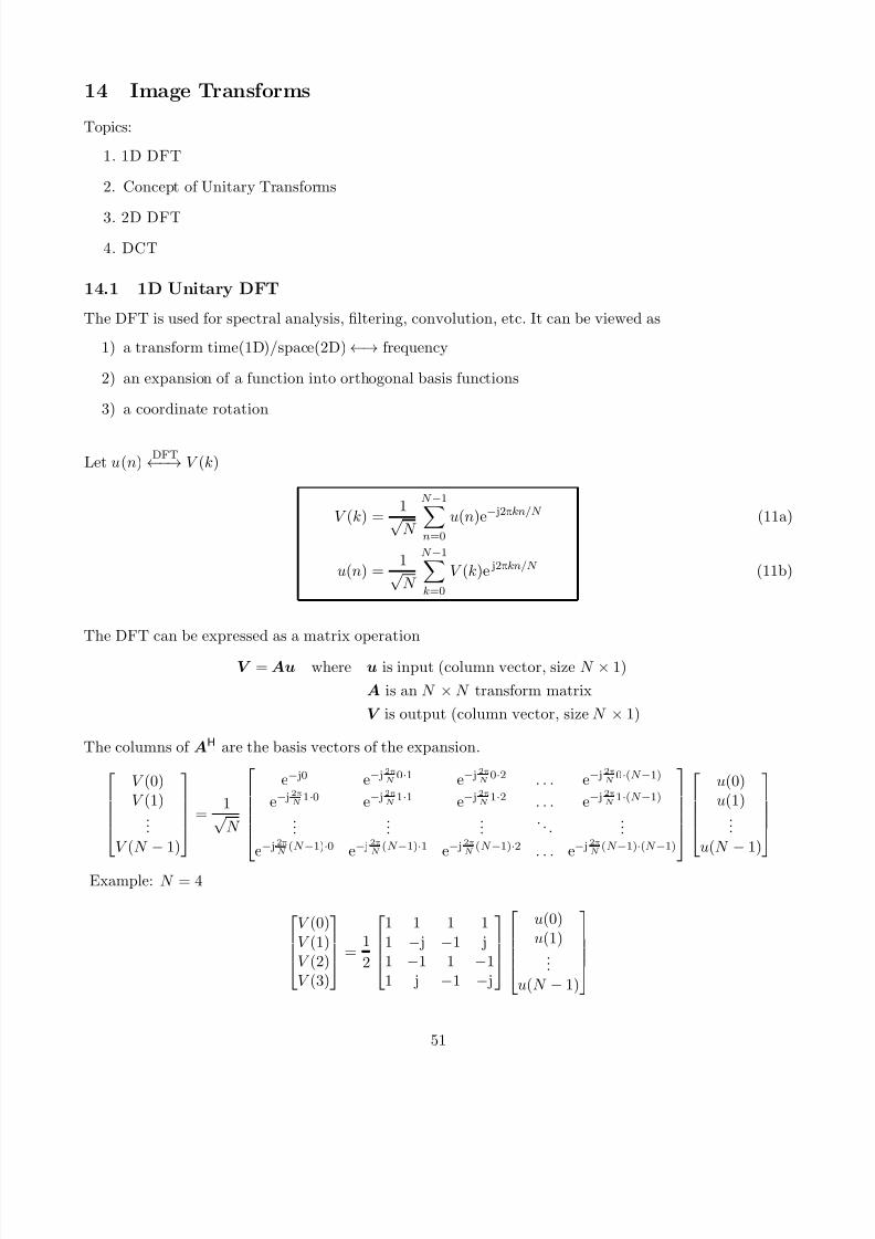
14 Image Transforms
Topics:
1. 1D DFT
2. Concept of Unitary Transforms
3. 2D DFT
4. DCT
14.1 1D Unitary DFT
The DFT is used for spectral analysis, filtering, convolution, etc. It can be viewed as
1) a transform time(1D)/space(2D) ←→ frequency
2) an expansion of a function into orthogonal basis functions
3) a coordinate rotation
Let u(n) DFT←−→ V (k)
V (k) = 1√
N
N −1n=0
u(n)e− j2πkn/N
u(n) = 1√
N
N −1k=0
V (k)e j2πkn/N
(11a)
(11b)
The DFT can be expressed as a matrix operation
V = Au where u is input (column vector, size N × 1)
A is an N × N transform matrix
V is output (column vector, size N × 1)
The columns of AH are the basis vectors of the expansion.
V (0)V (1)
...V (N − 1)
= 1√
N
e− j0 e− j 2πN
0·1 e− j 2πN
0·2 . . . e− j 2πN
0·(N −1)
e− j 2πN
1·0 e− j 2πN
1·1 e− j 2πN
1·2 . . . e− j 2πN
1·(N −1)
... ...
... . . .
...
e− j 2πN
(N −1)·0 e− j 2πN
(N −1)·1 e− j 2πN
(N −1)·2 . . . e− j 2πN
(N −1)·(N −1)
u(0)u(1)
...u(N − 1)
Example: N = 4
V (0)V (1)V (2)V (3)
=
1
2
1 1 1 11 − j −1 j1 −1 1 −11 j −1 − j
u(0)u(1)
...u(N − 1)
51
7/18/2019 Course Notes v17
http://slidepdf.com/reader/full/course-notes-v17 52/82
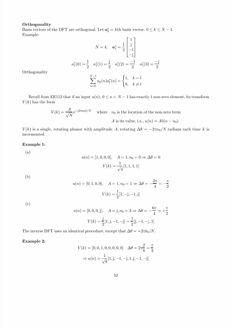
OrthogonalityBasis vectors of the DFT are orthogonal. Let a∗k = kth basis vector. 0 ≤ k ≤ N − 1.Example:
N = 4, a∗1 = 1
2
1 j−1
− j
a∗1(0) = 1
2 a∗1(1) =
j
2 a∗1(2) =
−1
2 a∗1(3) =
− j
2Orthogonality
N −1n=0
ak(n)a∗l (n) =
1, k = l
0, k = l
Recall from EE113 that if an input u(n), 0 ≤ n < N − 1 has exactly 1 non-zero element, its transform
V (k) has the form
V (k) = A
√ N e− j2πn0k/N where n0 is the location of the non-zero term
A is its value, i.e., u(n) = Aδ(n − n0)
V (k) is a single, rotating phasor with amplitude A, rotating ∆θ = −2πn0/N radians each time k isincremented.
Example 1:
(a)u(n) = [1, 0, 0, 0], A = 1, n0 = 0 ⇒ ∆θ = 0
V (k) = 1√
4[1, 1, 1, 1]
(b)
u(n) = [0, 1, 0, 0], A = 1, n0 = 1 ⇒ ∆θ = −2π
4 = −π
2
V (k) = 1
2[1, − j, −1, j]
(c)
u(n) = [0, 0, 0, j], A = j, n0 = 3 ⇒ ∆θ = −6π
4 = +
π
2
V (k) = j
2[1, j, −1, − j] =
1
2[j, −1, − j, 1]
The inverse DFT uses an identical procedure, except that ∆θ = +2πk0/N .
Example 2:
V (k) = [0, 0, 1, 0, 0, 0, 0, 0] ∆θ = 2π2
8 =
π
2
⇒ u(n) = 1√
8[1, j, −1, − j, 1, j, −1, − j]
52
7/18/2019 Course Notes v17
http://slidepdf.com/reader/full/course-notes-v17 53/82
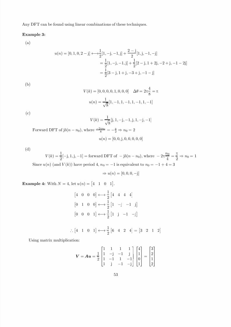
Any DFT can be found using linear combinations of these techniques.
Example 3:
(a)
u(n) = [0, 1, 0, 2
− j]
←→1
2
[1,
− j,
−1, j] +
2 − j
2
[1, j,
−1,
− j]
= 1
2[1, − j, −1, j] +
1
2[2 − j, 1 + 2j, −2 + j, −1 − 2j]
= 1
2[3 − j, 1 + j, −3 + j, −1 − j]
(b)
V (k) = [0, 0, 0, 0, 1, 0, 0, 0] ∆θ = 2π4
8 = π
u(n) = 1√
8[1, −1, 1, −1, 1, −1, 1, −1]
(c)V (k) =
1√ 8
[j, 1, − j, −1, j, 1, − j, −1]
Forward DFT of jδ(n − n0), where −2πn08 = −π
2 ⇒ n0 = 2
u(n) = [0, 0, j, 0, 0, 0, 0, 0]
(d)
V (k) = 1
2[− j, 1, j, −1] = forward DFT of − jδ(n − n0), where − 2π
n0
4 =
π
2 ⇒ n0 = 1
Since u(n) (and V (k)) have period 4, n0 = −1 is equivalent to n0 = −1 + 4 = 3
⇒ u(n) = [0, 0, 0, − j]
Example 4: With N = 4, let u(n) =
4 1 0 1
.
4 0 0 0
←→ 1
2
4 4 4 4
0 1 0 0 ←→ 1
2
1 − j −1 j
0 0 0 1 ←→ 1
2
1 j −1 − j
∴ 4 1 0 1 ←→ 126 4 2 4 = 3 2 1 2
Using matrix multiplication:
V = Au = 1
2
1 1 1 11 − j −1 j1 −1 1 −11 j −1 − j
4101
=
3212
53
7/18/2019 Course Notes v17
http://slidepdf.com/reader/full/course-notes-v17 54/82
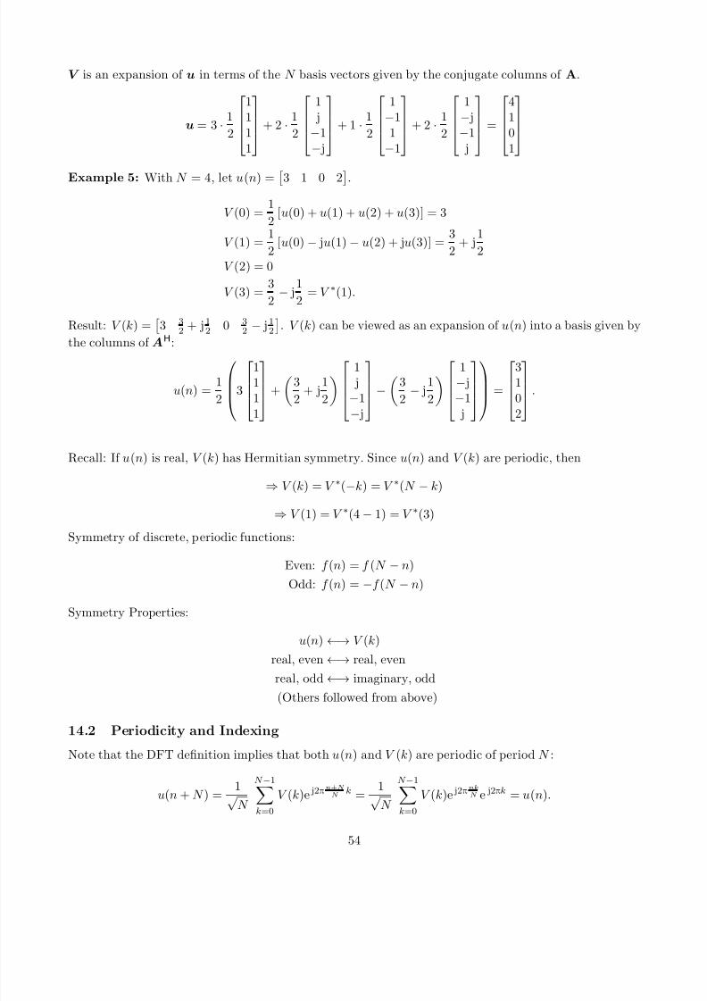
V is an expansion of u in terms of the N basis vectors given by the conjugate columns of A.
u = 3 · 1
2
1111
+ 2 · 1
2
1 j−1− j
+ 1 · 1
2
1−11
−1
+ 2 · 1
2
1− j−1 j
=
4101
Example 5: With N = 4, let u(n) = 3 1 0 2.V (0) =
1
2 [u(0) + u(1) + u(2) + u(3)] = 3
V (1) = 1
2 [u(0) − ju(1) − u(2) + ju(3)] =
3
2 + j
1
2V (2) = 0
V (3) = 3
2 − j
1
2 = V ∗(1).
Result: V (k) =
3 3
2 + j 12 0 3
2 − j 12
. V (k) can be viewed as an expansion of u(n) into a basis given by
the columns of AH:
u(n) = 1
2
3
1111
+
3
2 + j
1
2
1 j−1− j
−
3
2 − j
1
2
1− j−1 j
=
3102
.
Recall: If u(n) is real, V (k) has Hermitian symmetry. Since u(n) and V (k) are periodic, then
⇒ V (k) = V ∗(−k) = V ∗(N − k)
⇒V (1) = V ∗(4
−1) = V ∗(3)
Symmetry of discrete, periodic functions:
Even: f (n) = f (N − n)
Odd: f (n) = −f (N − n)
Symmetry Properties:
u(n) ←→ V (k)
real, even ←→ real, even
real, odd ←→ imaginary, odd
(Others followed from above)
14.2 Periodicity and Indexing
Note that the DFT definition implies that both u(n) and V (k) are periodic of period N :
u(n + N ) = 1√
N
N −1k=0
V (k)e j2πn+N N k =
1√ N
N −1k=0
V (k)e j2πnkN e j2πk = u(n).
54
7/18/2019 Course Notes v17
http://slidepdf.com/reader/full/course-notes-v17 55/82
In general, u(n) = u(n + N ), V (k) = V (k + N ), any integer.Example:
u(n) =
0 1 2 3 ⇒ u(n − 1) =
3 0 1 2
.
Although any window of length N is sufficient, by convention we use 0 ≤ n ≤ N − 1. This places theorigin on the left, not the center. Make sure you define vectors this way avery time you use functions such
as fft in Matlab.
14.3 DFT Properties
Parseval:N −1n=0
|u(n)|2 =N −1k=0
|V (k)|2 .
Reversal:If u(n) ↔ V (k), then u(−n) ↔ V (−k).
Note that if u(n) =
a b c d e f g h
thenu(−n) =
a h g f e d c b
.
Circular convolution:(u1 u2)(n) ↔ V 1(k)V 2(k).
Shift: If u(n) ↔ V (k), thenu(n − n0) ↔ e− j2πn0kV (k).
Exampleu(n) =
3 1 0 2
↔ V (k) =
3 32 + j 1
2 0 32 − j 1
2
then
u(n − 1) = 2 3 1 0 ↔ e− j2πk/4
V (k) = 3 1
2 − j3
2 0 1
2 + j3
2 .Shifting u(n) imposes a progressive phase term on V (k).
15 Unitary Transformations
The general form for a 1D unitary transformation is
V (k) =N −1n=0
u(n)a(k, n)
u(n) =
N −1k=0
V (k)a∗(k, n).
(12a)
(12b)
In matrix formV = Au,
where A is unitary , i.e.,A−1 = AH = (A∗)T .
55
7/18/2019 Course Notes v17
http://slidepdf.com/reader/full/course-notes-v17 56/82
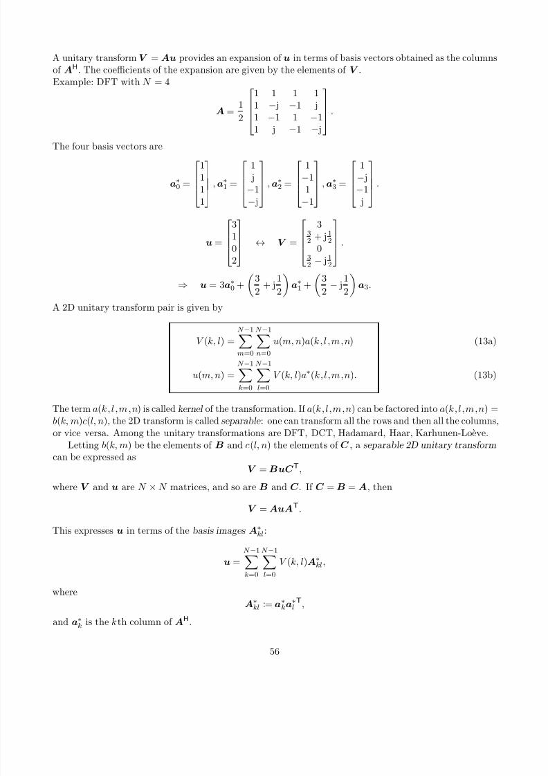
A unitary transform V = Au provides an expansion of u in terms of basis vectors obtained as the columns
of AH. The coefficients of the expansion are given by the elements of V .Example: DFT with N = 4
A = 1
2
1 1 1 11 − j −1 j1 −1 1 −11 j
−1
− j
.
The four basis vectors are
a∗0 =
1111
,a∗1 =
1 j−1− j
,a∗2 =
1−11
−1
,a∗3 =
1− j−1 j
.
u =
3102
↔ V =
332 + j 1
20
32
− j 1
2
.
⇒ u = 3a∗0 +
3
2 + j
1
2
a∗1 +
3
2 − j
1
2
a3.
A 2D unitary transform pair is given by
V (k, l) =
N −1m=0
N −1n=0
u(m, n)a(k,l ,m,n)
u(m, n) =N −1k=0
N −1l=0
V (k, l)a∗(k,l,m,n).
(13a)
(13b)
The term a(k,l ,m,n) is called kernel of the transformation. If a(k,l,m,n) can be factored into a(k,l,m,n) =b(k, m)c(l, n), the 2D transform is called separable : one can transform all the rows and then all the columns,
or vice versa. Among the unitary transformations are DFT, DCT, Hadamard, Haar, Karhunen-Loeve.Letting b(k, m) be the elements of B and c(l, n) the elements of C , a separable 2D unitary transform
can be expressed asV = BuC T,
where V and u are N × N matrices, and so are B and C . If C = B = A, then
V = AuAT.
This expresses u in terms of the basis images A∗kl:
u =N −1k=0
N −1l=0
V (k, l)A∗kl,
whereA∗kl := a
∗ka
∗lT,
and a∗k is the kth column of AH.
56
7/18/2019 Course Notes v17
http://slidepdf.com/reader/full/course-notes-v17 57/82
16 2D Unitary DFT
V (k, l) =
N −1m=0
N −1n=0
u(m, n)a(k,l ,m,n)
u(m, n) =N −1
k=0
N −1
l=0
V (k, l)a∗(k,l,m,n),
(14a)
(14b)
where the kernel of the transformation is
a(k,l ,m,n) = 1
N e− j2π
mk+nlN .
Since the kernel is factorable, the 2D DFT is separable, i.e., it can be implemented by 1D transforms of
rows, followed by 1D transform of columns (or vice versa).Example:
u(m, n) =
0 1 0 00 1 0 00 1 0 0
0 1 0 0
.
1D transform of columns :
⇒
0 2 0 00 0 0 00 0 0 00 0 0 0
.
1D transform of rows :
⇒
1 − j −1 j0 0 0 00 0 0 00 0 0 0
.
Example of 2D DFTs2D DFT, N = 4:
A = 1
2
1 1 1 11 − j −1 j1 −1 1 −11 j −1 − j
AH =
1
2
1 1 1 11 j −1 − j1 −1 1 −11 − j −1 j
,
and
a∗0 = 1
2
1111
, a∗1 = 1
2
1 j−1
− j
, etc.
Basis images (or basis maps):
A∗00 = a∗0a
∗0T =
1
4
1 1 1 11 1 1 11 1 1 11 1 1 1
, etc.
57
7/18/2019 Course Notes v17
http://slidepdf.com/reader/full/course-notes-v17 58/82
Example
u =
0 1 0 00 1 0 00 1 0 00 1 0 0
↔ V =
1 − j −1 j0 0 0 00 0 0 00 0 0 0
.
This means that we can express u as follows:
u = (1)A∗00 + (− j)A∗
01 + (−1)A∗02 + (j)A∗
03.
16.1 2D Periodic (Cyclic) Convolution
(u1 u2)(m, n) ↔ V 1(k, l)V 2(k, l).
For instance, u1(m, n) may be an image and u2(m, n) the impulse response of a digital filter, such as alow-pass filter. The filtering operation can be applied in the frequency domain by simply multiplyingV 1(k, l) and V 2(k, l) element by element, and then inverse transforming.
17 The Unitary Discrete Cosine Transform (DCT)
The DCT is a real transform, i.e., a real u(n) produces a real V (k). It can be obtained using a DFT. Most
fast DCT algorithms use FFTs. Of all unitary transforms, only the DFT is used more than the DCT.For a 1D sequence u(n), 0 ≤ n ≤ N − 1, the DCT V (k), 0 ≤ k ≤ N − 1, is given by
V = Cu,
where
C (k, n) =
1√ N
, k = 0, 0 ≤ n ≤ N − 1, 2N cos
π(2n+1)k
2N
, 1 ≤ k ≤ N − 1, 0 ≤ n ≤ N − 1.
As with the DFT, the DCT basis vectors are sinusoidal. The DCT is best understood in terms of a DFT
of a sequence of length 2N derived from u(n).The DFT implies a periodicity N in the sequence u(n). This periodicity can result in discontinuities
that do not reflect the nature of the signal u(n).u(n) =
1 2 3 4
. The periodic signal has discontinuities that cause energy to be placed in high-
frequency bins of V (k), the DFT of u(n).Principle behind DCT: Make the input symmetric by doubling the length of u(n) by defining u(n) of
period 2N , where u(n) = u(n), 0 ≤ n ≤ N − 1, and u(n) = u(2N − 1 − n) for N ≤ n ≤ 2N − 1. Thenon-unitary definition of the DCT is thus:
V (k) =N −1
n=0
2u(n)cos
2πk
n + 1
2
2N
, 0 ≤ k ≤ N − 1.
The inverse transform is:
u(n) = 1
2N
V (0) +
N −1k=0
2V (k)cos
2πk
n + 1
2
2N
.
58
7/18/2019 Course Notes v17
http://slidepdf.com/reader/full/course-notes-v17 59/82
Note that V (0) is considered separately because in a symmetric DFT of length 2N the DC element isrepresented only once: V (1) = V (2N − 1), V (2) = V (2N − 2), . . ., V (0) = V (0). The 1D unitary DCT isgiven by:
V (k) = α(k)
N −1n=0
u(n)cos
π(2n + 1)k
2N
, 0 ≤ k ≤ N − 1
u(n) =
N
−1
n=0
α(k)V (k)cosπ(2n + 1)k2N
, 0 ≤ n ≤ N − 1
α(0) = 1√
N , α(k) =
2
N , 1 ≤ k ≤ N − 1.
(15a)
(15b)
(15c)
The 2D unitary DCT is given by:
V (k, l) = α(k)α(l)N −1m=0
N −1n=0
u(m, n)cos
π(2m + 1)k
2N
cos
π(2n + 1)l
2N
u(m, n) =N −1
k=0
N −1
l=0
α(k)α(l)V (k, l)cosπ(2m + 1)k
2N cosπ(2n + 1)l
2N .
(16a)
(16b)
For signals that generate a smooth u(n) the DCT is well localized. In general, the N → 2N mappingimplicit in the DCT gives smoother sequences than the periodic N extension of the DFT. This is why the
DCT has better energy compression for most sequences.Example:
0.65 0.27 −0.27 −0.65
has DCT 0 1 0 0
and DFT 0 0.46 − j0.46 0 0.46 + j0.46 .
Because 0.65 0.27 −0.27 −0.65 −0.65 −0.27 0.27 0.65
is smooth under 2N periodicity, its DCT is compact.Example
1 1 1 1
has DFT and DCT equal to 2 0 0 0
.
Example
1 0 0 0has DCT equal to
0.5 0.65 0.5 0.27
and DFT 0.5 0.5 0.5 0.5
.
The DCT of an impulse is not DC.
59
7/18/2019 Course Notes v17
http://slidepdf.com/reader/full/course-notes-v17 60/82
The DFT kernel is symmetric, i.e., exchanging n with k will not affect the transform. In the DCT the
kernel is not symmetric with respect to n and k.Example: mid-frequency
1 0 −1 0
has DCT
0 0.92 1
−0.38
and DFT 0 1 0 1
.
Example: high-frequency 1 −1 1 −1
has DCT
0 0.765 0 1.848
and DFT 0 0 2 0
.
For signals whose periodic extension is smooth, the energy localization with the DFT seems to be
better than with the DCT. This is because the assumption of periodicity of the DFT does not apply withthe DCT.
For the DCT, C = C T and the expansion using the DCT is fundamentally different from the expansion
using the IDCT.
60

7/18/2019 Course Notes v17
http://slidepdf.com/reader/full/course-notes-v17 61/82
18 Image Enhancement
Image enhancement techniques are used to improve the perception of images to human observers. Thereare subjective and objective measures of quality.
The image may also be processed for further machine-based analysis.Among image enhancements techniques are
1. Contrast enhancement
(a) Histogram (gray scale) modification
(b) High-pass (linear) filtering
(c) Homomorphic processing
2. Denoising and noise smoothing (background noise, Gaussian noise, salt-and-pepper noise, specklenoise, quantization noise)
(a) Low-pass (linear) filtering
(b) Median (nonlinear) filtering
(c) Out-of-range pixel smoothing (nonlinear)
3. Edge detection
(a) Gradient-based edge detection
(b) Laplacian-based edge detection
18.1 Contrast Enhancement
18.1.1 Histogram modification
Let u(m, n) be the intensity level of pixel (m, n) of a given image. Histogram modification allows one to
change the range of values taken on by the intensity function, thereby improving the contrast of the image.
Let y (m, n) be the result of the transformation
y = T [u].
As an example, consider the 4 × 4 image with intensities given by
u =
3 3 4 52 3 4 42 3 4 43 3 4 5
,
where 0 is black and 7 is white. The histogram and the cumulative histogram of the image are given by
u p(u) P (u)
0 0 01 0 02 2 23 6 84 6 145 2 166 0 167 0 16
61

7/18/2019 Course Notes v17
http://slidepdf.com/reader/full/course-notes-v17 62/82
Assume that ideally we would like to have a cumulative histogram given by
y P d(y)
0 21 42 63 8
4 105 126 147 16
The transformation from u to y can now be obtained as follows:
1. Pick a value of u
2. Look up P (u)
3. Find P d(y) that is closest to P (u)
4. Choose the corresponding y
In our example:
1. u = 0 → P (u) = 0 → P d(y) = 2 → y = 0
2. u = 1 → P (u) = 0 → P d(y) = 2 → y = 0
3. u = 2 → P (u) = 2 → P d(y) = 2 → y = 0
4. u = 3 → P (u) = 8 → P d(y) = 8 → y = 3
5. u = 4 → P (u) = 14 → P d(y) = 14 → y = 6
6. u = 5 → P (u) = 16 → P d(y) = 16 → y = 7
7. u = 6 → P (u) = 16 → P d(y) = 16 → y = 7
8. u = 7 → P (u) = 16 → P d(y) = 16 → y = 7
which corresponds to the transformation
u y
0 01 02 0
3 34 65 76 77 7
62
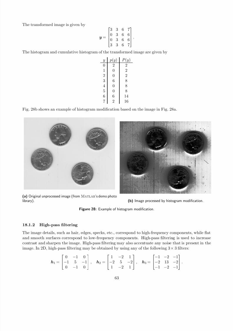
7/18/2019 Course Notes v17
http://slidepdf.com/reader/full/course-notes-v17 63/82
The transformed image is given by
y =
3 3 6 70 3 6 60 3 6 63 3 6 7
.
The histogram and cumulative histogram of the transformed image are given by
y p(y) P (y)
0 2 21 0 22 0 23 6 84 0 85 0 86 6 147 2 16
Fig. 28b shows an example of histogram modification based on the image in Fig. 28a.
(a) Original unprocessed image (from Matlab’s demo photolibrary). (b) Image processed by histogram modification.
Figure 28: Example of histogram modification.
18.1.2 High-pass filtering
The image details, such as hair, edges, specks, etc., correspond to high-frequency components, while flatand smooth surfaces correspond to low-frequency components. High-pass filtering is used to increasecontrast and sharpen the image. High-pass filtering may also accentuate any noise that is present in the
image. In 2D, high-pass filtering may be obtained by using any of the following 3 × 3 filters:
h1 =
0 −1 0−1 5 −10 −1 0
, h2 =
1 −2 1−2 5 −21 −2 1
, h3 =
−1 −2 −1−2 13 −2−1 −2 −1
.
63
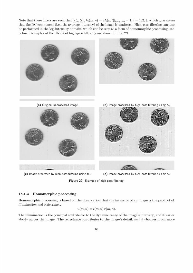
7/18/2019 Course Notes v17
http://slidepdf.com/reader/full/course-notes-v17 64/82
Note that these filters are such that
m
n hi(m, n) = H i(k, l)|k=0,l=0 = 1, i = 1, 2, 3, which guarantees
that the DC component (i.e., the average intensity) of the image is unaltered. High-pass filtering can also
be performed in the log-intensity domain, which can be seen as a form of homomorphic processing, seebelow. Examples of the effects of high-pass filtering are shown in Fig. 29.
(a) Original unprocessed image. (b) Image processed by high-pass filtering using h1.
(c) Image processed by high-pass filtering using h2. (d) Image processed by high-pass filtering using h3.
Figure 29: Example of high-pass filtering.
18.1.3 Homomorphic processing
Homomorphic processing is based on the observation that the intensity of an image is the product of illumination and reflectance ,
u(m, n) = i(m, n) r(m, n).
The illumination is the principal contributor to the dynamic range of the image’s intensity, and it varies
slowly across the image. The reflectance contributes to the image’s detail, and it changes much more
64
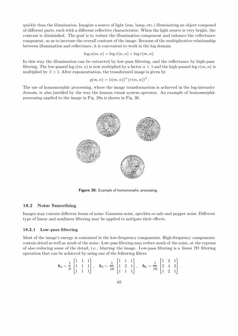
7/18/2019 Course Notes v17
http://slidepdf.com/reader/full/course-notes-v17 65/82
quickly than the illumination. Imagine a source of light (sun, lamp, etc.) illuminating an object composed
of different parts, each with a different reflective characteristic. When the light source is very bright, thecontrast is diminished. The goal is to reduce the illumination component and enhance the reflectancecomponent, so as to increase the overall contrast of the image. Because of the multiplicative relationshipbetween illumination and reflectance, it is convenient to work in the log domain
log u(m, n) = log i(m, n) + log r(m, n).
In this way the illumination can be extracted by low-pass filtering, and the reflectance by high-passfiltering. The low-passed log i(m, n) is now multiplied by a factor α < 1 and the high-passed log r(m, n) is
multiplied by β > 1. After exponentiation, the transformed image is given by
y(m, n) = (i(m, n))α (r(m, n))β .
The use of homomorphic processing, where the image transformation is achieved in the log-intensitydomain, is also justified by the way the human visual system operates. An example of homomorphicprocessing applied to the image in Fig. 28a is shown in Fig. 30.
Figure 30: Example of homomorphic processing.
18.2 Noise Smoothing
Images may contain different forms of noise: Gaussian noise, speckles or salt-and-pepper noise. Differenttype of linear and nonlinear filtering may be applied to mitigate their effects.
18.2.1 Low-pass filtering
Most of the image’s energy is contained in the low-frequency components. High-frequency componentscontain detail as well as much of the noise. Low-pass filtering may reduce much of the noise, at the expense
of also reducing some of the detail, i.e., blurring the image. Low-pass filtering is a linear 2D filteringoperation that can be achieved by using one of the following filters
h4 = 1
9
1 1 1
1 1 11 1 1
, h5 =
1
10
1 1 1
1 2 11 1 1
, h6 =
1
16
1 2 1
2 4 21 2 1
.
65
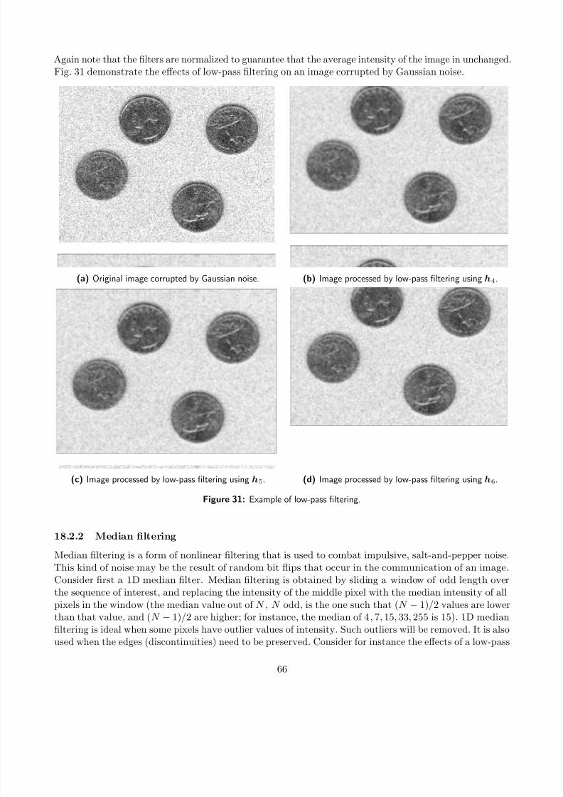
7/18/2019 Course Notes v17
http://slidepdf.com/reader/full/course-notes-v17 66/82
Again note that the filters are normalized to guarantee that the average intensity of the image in unchanged.
Fig. 31 demonstrate the effects of low-pass filtering on an image corrupted by Gaussian noise.
(a) Original image corrupted by Gaussian noise. (b) Image processed by low-pass filtering using h4.
(c) Image processed by low-pass filtering using h5. (d) Image processed by low-pass filtering using h6.
Figure 31: Example of low-pass filtering.
18.2.2 Median filtering
Median filtering is a form of nonlinear filtering that is used to combat impulsive, salt-and-pepper noise.This kind of noise may be the result of random bit flips that occur in the communication of an image.Consider first a 1D median filter. Median filtering is obtained by sliding a window of odd length overthe sequence of interest, and replacing the intensity of the middle pixel with the median intensity of allpixels in the window (the median value out of N , N odd, is the one such that (N − 1)/2 values are lowerthan that value, and (N − 1)/2 are higher; for instance, the median of 4, 7, 15, 33, 255 is 15). 1D median
filtering is ideal when some pixels have outlier values of intensity. Such outliers will be removed. It is alsoused when the edges (discontinuities) need to be preserved. Consider for instance the effects of a low-pass
66
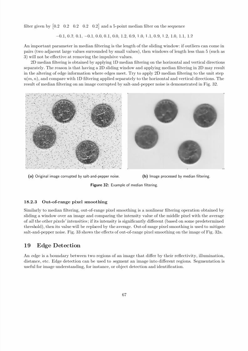
7/18/2019 Course Notes v17
http://slidepdf.com/reader/full/course-notes-v17 67/82
filter given by
0.2 0.2 0.2 0.2 0.2
and a 5-point median filter on the sequence
−0.1, 0.2, 0.1, −0.1, 0.0, 0.1, 0.0, 1.2, 0.9, 1.0, 1.1, 0.9, 1.2, 1.0, 1.1, 1.2
An important parameter in median filtering is the length of the sliding window: if outliers can come inpairs (two adjacent large values surrounded by small values), then windows of length less than 5 (such as3) will not be effective at removing the impulsive values.
2D median filtering is obtained by applying 1D median filtering on the horizontal and vertical directionsseparately. The reason is that having a 2D sliding window and applying median filtering in 2D may result
in the altering of edge information where edges meet. Try to apply 2D median filtering to the unit stepu(m, n), and compare with 1D filtering applied separately to the horizontal and vertical directions. The
result of median filtering on an image corrupted by salt-and-pepper noise is demonstrated in Fig. 32.
(a) Original image corrupted by salt-and-pepper noise. (b) Image processed by median filtering.
Figure 32: Example of median filtering.
18.2.3 Out-of-range pixel smoothing
Similarly to median filtering, out-of-range pixel smoothing is a nonlinear filtering operation obtained by
sliding a window over an image and comparing the intensity value of the middle pixel with the averageof all the other pixels’ intensities ; if its intensity is significantly different (based on some predeterminedthreshold), then its value will be replaced by the average. Out-of-range pixel smoothing is used to mitigate
salt-and-pepper noise. Fig. 33 shows the effects of out-of-range pixel smoothing on the image of Fig. 32a.
19 Edge DetectionAn edge is a boundary between two regions of an image that differ by their reflectivity, illumination,distance, etc. Edge detection can be used to segment an image into different regions. Segmentation isuseful for image understanding, for instance, or object detection and identification.
67
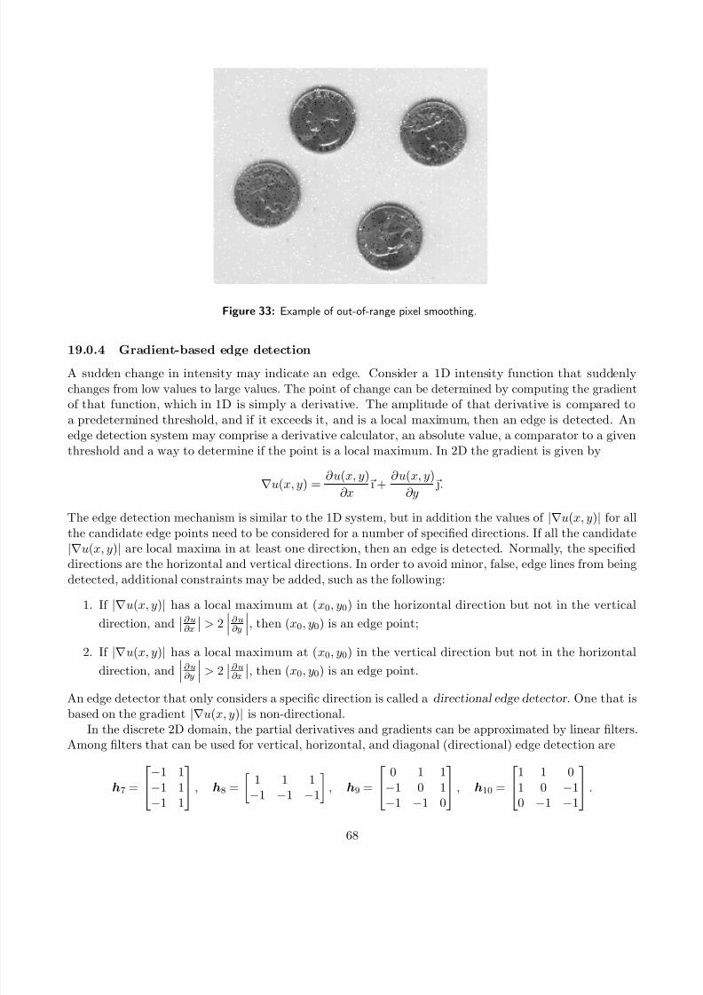
7/18/2019 Course Notes v17
http://slidepdf.com/reader/full/course-notes-v17 68/82
Figure 33: Example of out-of-range pixel smoothing.
19.0.4 Gradient-based edge detection
A sudden change in intensity may indicate an edge. Consider a 1D intensity function that suddenlychanges from low values to large values. The point of change can be determined by computing the gradient
of that function, which in 1D is simply a derivative. The amplitude of that derivative is compared toa predetermined threshold, and if it exceeds it, and is a local maximum, then an edge is detected. Anedge detection system may comprise a derivative calculator, an absolute value, a comparator to a giventhreshold and a way to determine if the point is a local maximum. In 2D the gradient is given by
∇u(x, y) = ∂ u(x, y)
∂x ı +
∂u(x, y)
∂y .
The edge detection mechanism is similar to the 1D system, but in addition the values of |∇u(x, y)| for allthe candidate edge points need to be considered for a number of specified directions. If all the candidate|∇u(x, y)| are local maxima in at least one direction, then an edge is detected. Normally, the specifieddirections are the horizontal and vertical directions. In order to avoid minor, false, edge lines from beingdetected, additional constraints may be added, such as the following:
1. If |∇u(x, y)| has a local maximum at (x0, y0) in the horizontal direction but not in the vertical
direction, and∂u∂x
> 2∂u∂y , then (x0, y0) is an edge point;
2. If |∇u(x, y)| has a local maximum at (x0, y0) in the vertical direction but not in the horizontal
direction, and∂u∂y
> 2
∂u∂x
, then (x0, y0) is an edge point.
An edge detector that only considers a specific direction is called a directional edge detector . One that isbased on the gradient |∇u(x, y)| is non-directional.
In the discrete 2D domain, the partial derivatives and gradients can be approximated by linear filters.Among filters that can be used for vertical, horizontal, and diagonal (directional) edge detection are
h7 =
−1 1−1 1−1 1
, h8 =
1 1 1−1 −1 −1
, h9 =
0 1 1−1 0 1−1 −1 0
, h10 =
1 1 0
1 0 −10 −1 −1
.
68
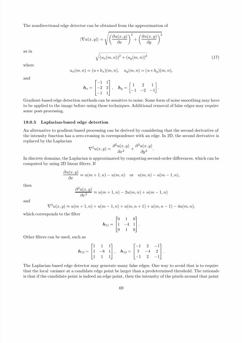
7/18/2019 Course Notes v17
http://slidepdf.com/reader/full/course-notes-v17 69/82
The nondirectional edge detector can be obtained from the approximation of
|∇u(x, y)| =
∂ u(x, y)
∂x
2
+
∂ u(x, y)
∂y
2
as in
(ux
(m, n))2 + (uy
(m, n))2 (17)
whereux(m, n) = (u ∗ hx)(m, n), uy(m, n) = (u ∗ hy)(m, n),
and
hx =
−1 1−2 2−1 1
, hy =
1 2 1−1 −2 −1
.
Gradient-based edge detection methods can be sensitive to noise. Some form of noise smoothing may have
to be applied to the image before using these techniques. Additional removal of false edges may require
some post-processing.
19.0.5 Laplacian-based edge detection
An alternative to gradient-based processing can be derived by considering that the second derivative of the intensity function has a zero-crossing in correspondence with an edge. In 2D, the second derivative isreplaced by the Laplacian
∇2u(x, y) = ∂ 2u(x, y)
∂x2 +
∂ 2u(x, y)
∂y 2 .
In discrete domains, the Laplacian is approximated by computing second-order differences, which can becomputed by using 2D linear filters. If
∂ u(x, y)
∂x ≈u(m + 1, n)
−u(m, n) or u(m, n)
−u(m
−1, n),
then∂ 2u(x, y)
∂x2 ≈ u(m + 1, n) − 2u(m, n) + u(m − 1, n)
and∇2u(x, y) ≈ u(m + 1, n) + u(m − 1, n) + u(m, n + 1) + u(m, n − 1) − 4u(m, n),
which corresponds to the filter
h11 =
0 1 0
1 −4 10 1 0
.
Other filters can be used, such as
h12 =
1 1 1
1 −8 11 1 1
, h13 =
−1 2 −1
2 −4 2−1 2 −1
.
The Laplacian-based edge detector may generate many false edges. One way to avoid that is to requirethat the local variance at a candidate edge point be larger than a predetermined threshold. The rationale
is that if the candidate point is indeed an edge point, then the intensity of the pixels around that point
69

7/18/2019 Course Notes v17
http://slidepdf.com/reader/full/course-notes-v17 70/82
should vary greatly. The variance should be small if the candidate point is simply an outlier. The variance
over a (2M + 1) × (2M + 1) window is computed as follows:
σ2(m, n) = 1
(2M + 1)2
m+M k=m−M
n+M l=n−M
(u(k, l) − µ(k, l))2 ,
whereµ(m, n) =
1
(2M + 1)2
m+M k=m−M
n+M l=n−M
u(k, l)
is the sample mean. The value of M is a design parameter, and is typically M = 2. The threshold willdepend on the nature of the image. Examples of edge detection are shown in Fig. 34
70
7/18/2019 Course Notes v17
http://slidepdf.com/reader/full/course-notes-v17 71/82
(a) Original unprocessed image(from Matlab’s demo photo li-brary).
(b) Image processed by gradient-based edge detection using h7.
(c) Image processed by gradient-based edge detection using h8.
(d) Image processed by gradient-based edge detection using h9.
(e) Image processed by gradient-based edge detection using h10.
(f) Image processed by gradient-based edge detection using (17).
(g) Image processed by Laplacian-based edge detection using h11, withno zero-crossing detection or variancethresholding.
(h) Image processed by Laplacian-based edge detection using h12, withno zero-crossing detection or variancethresholding.
Figure 34: Example of edge detection.
71
7/18/2019 Course Notes v17
http://slidepdf.com/reader/full/course-notes-v17 72/82
20 Image Compression and Coding
Goal: To reduce the number of bits needed to encode an image by eliminating redundancy.Current and future application examples:
Application Raw data volume (1 Mibit = 220 bits)
Color image (256 × 256, 24-bit color) 1.5Mibit
Color video, 1920 × 1080, 24-bit color, 60 fps 2.98 Gibit/sDigital Radiology Facility 64 Mibit/image, 1800 images per monthSAR Facility 800 Mibit/image, 5 to 10 images per dayFax 2 Mibit/page
Almost all compression techniques use one or more of the following principles:
1. Resources, i.e., storage space and transmission time, will be conserved if one uses short messages tocommunicate the occurrence of common events
2. Pixels within a given region are often correlated
3. If loss must occur, discard information less vital to the image
Compression techniques are divided into two classes
1. Reversible, error-free, distortionless: all information is preserved, complete reconstruction is possible.
Typical compression 3 : 1
2. Irreversible, lossy: some information is lost. Typical compression 20 : 1 for single images.
20.1 Information Theory Background
The information of a random event with probability P (E) is
I (E) =−
log P (E).
The base of the logarithm determines the units of information, a bit if the base is 2, a nat if the base is e.Example: E = {coin toss = heads}
P (E) = 1
2 ⇒ I (E) = − log2
1
2 = 1bit.
Now consider an information source with an alphabet of L possible symbols, each with probability pi,i = 0, 1, . . . , L − 1,
L−1i=0
pi = 1.
If M 1 symbols are generated by this source, symbol i will appear M pi times. The informationcontributed by symbol i is
I i = −Mpi log2 pi bits.
The total information in the string of M symbols is
I = −M L−1i=0
pi log2 pi.
72
7/18/2019 Course Notes v17
http://slidepdf.com/reader/full/course-notes-v17 73/82
The average information per symbol, H is
H = −L−1i=0
pi log2 pi = Entropy.
According to Shannon’s noiseless coding theorem, it is always possible to devise a code with an average of
B bits per symbol where
H ≤ B ≤ H + 1
n,
where n is the number of symbols encoded at one time. Usually n = 1.
20.2 Huffman Coding
Huffman Coding is a common, reversible image compression technique that encodes one symbol at a time
and results in a variable-length code with the lowest possible bit rate.To generate a Huffman codebook
1. Map initial symbols to symbol nodes and order based on symbol probabilities
2. Combine two symbol nodes having the lowest probabilities into a new symbol node, using 0 and 1 tolink the new node to the former symbols
3. Repeat until only two symbol nodes remain.
20.3 How to generate a Huffman tree
Let us use an example. Assume your source’s alphabet is given in the following table, together with the
symbols’ probabilities:
Symbol Probability
a 0.1
b 0.4c 0.04d 0.1e 0.07f 0.29
Let’s first rank the symbols by descending probability and create a node for each symbol (which willbecome a leaf in the tree):
73
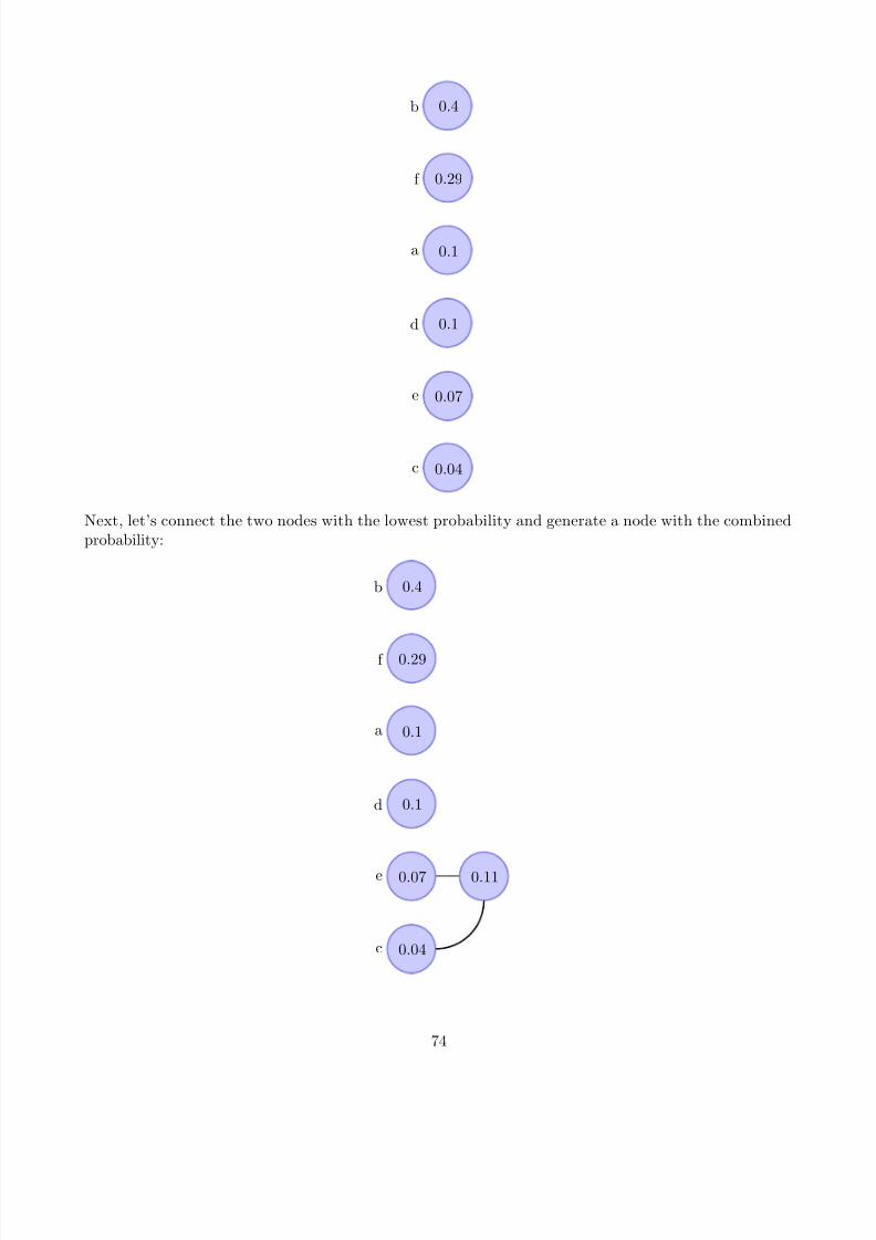
7/18/2019 Course Notes v17
http://slidepdf.com/reader/full/course-notes-v17 74/82
0.4b
0.29f
0.1a
0.1d
0.07e
0.04c
Next, let’s connect the two nodes with the lowest probability and generate a node with the combinedprobability:
0.4b
0.29f
0.1a
0.1d
0.07e
0.04c
0.11
74
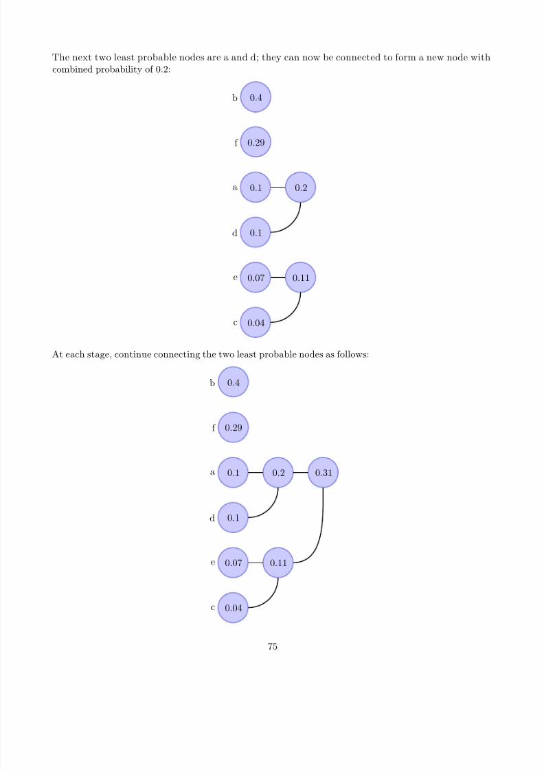
7/18/2019 Course Notes v17
http://slidepdf.com/reader/full/course-notes-v17 75/82
The next two least probable nodes are a and d; they can now be connected to form a new node withcombined probability of 0.2:
0.4b
0.29f
0.1a
0.1d
0.07e
0.04c
0.11
0.2
At each stage, continue connecting the two least probable nodes as follows:
0.4b
0.29f
0.1a
0.1d
0.07e
0.04c
0.11
0.2 0.31
75
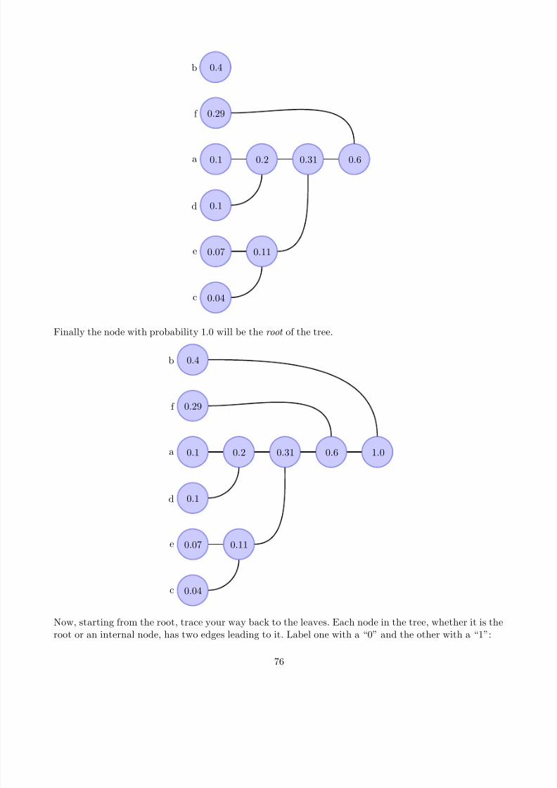
7/18/2019 Course Notes v17
http://slidepdf.com/reader/full/course-notes-v17 76/82
0.4b
0.29f
0.1a
0.1d
0.07e
0.04c
0.11
0.2 0.31 0.6
Finally the node with probability 1.0 will be the root of the tree.
0.4b
0.29f
0.1a
0.1d
0.07e
0.04c
0.11
0.2 0.31 0.6 1.0
Now, starting from the root, trace your way back to the leaves. Each node in the tree, whether it is the
root or an internal node, has two edges leading to it. Label one with a “0” and the other with a “1”:
76
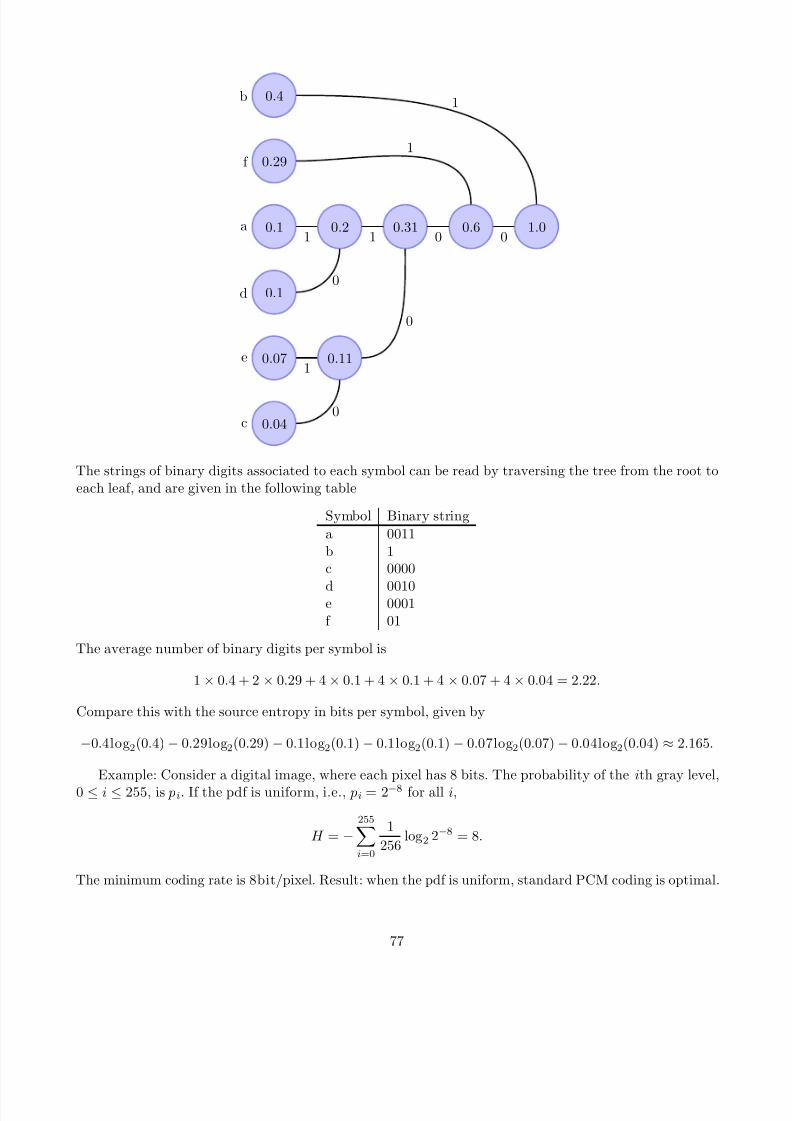
7/18/2019 Course Notes v17
http://slidepdf.com/reader/full/course-notes-v17 77/82
0.4b
0.29f
0.1a
0.1d
0.07e
0.04c
0.111
0
0.21
0
0.311
0
0.60
1
1.00
1
The strings of binary digits associated to each symbol can be read by traversing the tree from the root to
each leaf, and are given in the following table
Symbol Binary string
a 0011b 1c 0000
d 0010e 0001f 01
The average number of binary digits per symbol is
1 × 0.4 + 2 × 0.29 + 4 × 0.1 + 4 × 0.1 + 4 × 0.07 + 4 × 0.04 = 2.22.
Compare this with the source entropy in bits per symbol, given by
−0.4log2(0.4) − 0.29log2(0.29) − 0.1log2(0.1) − 0.1log2(0.1) − 0.07log2(0.07) − 0.04log2(0.04) ≈ 2.165.
Example: Consider a digital image, where each pixel has 8 bits. The probability of the ith gray level,0 ≤ i ≤ 255, is pi. If the pdf is uniform, i.e., pi = 2−8 for all i,
H = −255i=0
1
256 log2 2−8 = 8.
The minimum coding rate is 8bit/pixel. Result: when the pdf is uniform, standard PCM coding is optimal.
77
7/18/2019 Course Notes v17
http://slidepdf.com/reader/full/course-notes-v17 78/82
Example: Suppose the image pdf is
pi =
2−7, 0 ≤ i ≤ 127,
0, 128 ≤ i ≤ 255.
Then H = 7, and sending 8 bit/pixel is not optimal.If an image having M bits per pixel has entropy H , the minimum possible distortionless coding scheme
uses H bits per pixel, and the maximum compression rate is
C = M
H ,
and the efficiency of a code using B bits per pixel is
efficiency = H
B.
Note that although the codewords are of variable length, they are uniquely decodable. No end-of-wordcode needs to be sent.
Problem: if M different symbols are possible, there are L codewords, with the longest codeword having
length L.
In the modified Huffman coding , the first L1 symbols are Huffman coded, with symbol i given byi = qL1 + j.
20.4 Run-length Coding (RLC)
RLC is especially good for documents, drawings, and other two-tone images. RLC is the basis for faxtransmission.
Principle: Encode the lengths of runs of consecutive pixels. Possibilities include:
1. Encoding the number of zeros between two consecutive 1s (good when P (1) 1)
2. Encoding the distance to the next 1 → 0 or 0 → 1 transition.
Often the run-lengths themselves are Huffman coded.
20.5 Bit-plane Encoding
Consider an 8-bit image as 8 separate two-tone images. Encode each plane separately.
20.6 Distortion Function
In communication, the rate distortion function, RD, gives the minimum possible coding rate for a given
channel-induced distortion. In image compression, the channel is the image compression/decompression
process. A quantizer that achieves RD is called a Shannon quantizer .Examples:
1. Binary source: d = 1 if coding error occurs, d = 0 is no coding errors occur, p(1) = 12 . Note: if D = 0, the minimum rate is 1 bit/symbol, if D = 0.5, RD = 0.
2. Gaussian source with variance σ 2.
RD = max
0,
1
2 log2
σ2
D
Note: if we accept D = σ2, no information needs to be sent.
78
7/18/2019 Course Notes v17
http://slidepdf.com/reader/full/course-notes-v17 79/82
21 Transform Coding and Compression
Steps:
1. Transform u(m, n) to get V (k, l)
2. Quantization: Each element of V (k, l) is called a coefficient. Each coefficient is quantized using nk,l
bits, where nk,l
is larger for (k, l
) where the variance of V
(k, l
), σ
2
k,l, is large. The value
nk.l is called
the bit allocation.
Example of bit allocation with N = 4, coded as 0.5bit/pixel, i.e., 8 bits per 4 × 4 block.
3 2 0 02 1 0 00 0 0 00 0 0 0
The coded image is V (k, l).
3. Send V (k, l) to the receiver.
4. Inverse-transform V (k, l) to get u(m, n).
22 The JPEG Standard
JPEG = Joint Photographic Expert Group, representatives form industry and academia from all overthe world. “Joint” refers to ISO (international Standardization Organization) and CCITT (ComiteConsultatif International Telephonique et Telegraphique, now ITU-T, International Telegraph Union,Telecommunication Standardization Sector).Goal: A compression standard ensuring compatibility, universality, etc.
There are several modes (progressive, lossless, etc.) in JPEG. We consider only the basic lossy mode.The algorithm (assume the image consists of M -bit integers)
1. Break the image up into non-overlapping 8 × 8 blocks.
2. For each block u(m, n), take the 8 × 8 DCT:
u(m, n) → V (k, l).
3. Quantize each DCT coefficient. The quantization step size for each (k, l) is stored in a look-up table
as q (k, l), 1 ≤ q (k, l) ≤ 255:
V (k, l) = integerround
V (k, l)
q (k, l)
,
where q (k, l) is determined by the just noticeable threshold: if the contribution of V (k, l) will not be
noticed, then V (k, l) = 0. The DC coefficient, V (0, 0), is then converted to a differential value:
∆V = V (0, 0)
block n− V (0, 0)
block n−1
4. The 64 DCT coefficients are then mapped to a 1D vector of length 64 by using a zig-zag approach.This orders V (k.l) in approximate order of increasing spatial frequency. Many coefficients of V (k, l)are zero or near zero.
79
7/18/2019 Course Notes v17
http://slidepdf.com/reader/full/course-notes-v17 80/82
5. The 1D vector of length L1 = 64 is run-length coded (DC element excluded). Each non-zero value is
represented by two symbols:
Symbol 1 : (Run length, size S ), where S is the number of bits used to code symbol 2;
Symbol 2 : Amplitude, axpressed as an S -bit number. For M = 8-bit images, shifted to a range−127 ≤ p ≤ 128, the maximum possible DCT coefficient’s amplitude is 1
8 × 64 × 128 = 1024 ⇒S max = M + 3.
6. Symbol is entropy-coded using modified Huffman code.
Color images contain three components, one component of luminance (gray scale), and two components of
chrominance . In JPEG, chrominance is coded with less precision than luminance.JPEG performance for color images depends on quantization table, image stats, etc.):
0.25 to 0.5 bits per pixel moderate quality, but degradationnoticeable
≈ 1 bit per pixel excellent, acceptable for most uses1.5 to 2 bits per pixel usually indistinguishable from origi-
nal
Other JPEG features include
1. Progressive encoding: sen most important information first. Two options
(a) Send most important DCT coefficient first
(b) Send most significant bits of all DCT coefficients first
2. Lossless predictive coding algorithm based on 2D prediction
23 Video Compression
1. Intraframe techniques compress single images and use spatial redundancy to reduce the bit rate
2. Interframe techniques use temporal redundancies between frames.
A full video compression scheme incorporates both types of redundancy.Video applications can be classified as
• Symmetric : compression and decompression are performed with equal frequency – Example: videoconferencing, video telephone, etc.
• Asymmetric : compress only once – Example: movies, electronic publishing, etc.
The goal of most video compression schemes is often a rate of about 1.5 Mibit/s. This is a good rate for
LANs, existing communication channels, etc. One of the most recent standards is MPEG (motion picture
experts group). Achieved and projected bit rates (for 30 frames/s, non-interlaced) are:
Resolution Compressed bit rate (Mibit/s)352 × 240 ≈ 1.5 (VHS-like quality)720 × 489 ≈ 7.51920 × 1080 (HDTV) ≈ 30
80
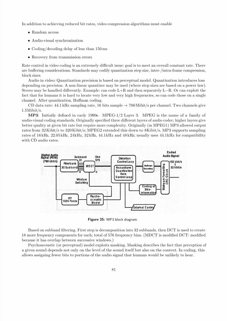
7/18/2019 Course Notes v17
http://slidepdf.com/reader/full/course-notes-v17 81/82
In addition to achieving reduced bit rates, video compression algorithms must enable
• Random access
• Audio-visual synchronization
• Coding/decoding delay of less than 150 ms
• Recovery from transmission errors
Rate control in video coding is an extremely difficult issue: goal is to meet an overall constant rate. There
are buffering considerations. Standards may codify quantization step size, inter-/intra-frame compression,block sizes.
Audio in video: Quantization precision is based on perceptual model. Quantization introduces lossdepending on precision. A non-linear quantizer may be used (where step sizes are based on a power law).Stereo may be handled differently. Example: can code L+R and then separately L−R. Or can exploit thefact that for humans it is hard to locate very low and very high frequencies, so can code those on a single
channel. After quantization, Huffman coding.CD data rate: 44.1 kHz sampling rate, 16 bits sample → 700 Mibit/s per channel. Two channels give
1.5Mibit/s.MP3: Initially defined in early 1990s. MPEG-1/2 Layer 3. MPEG is the name of a family of audio-visual coding standards. Originally specified three different layers of audio codec; higher layers give
better quality at given bit rate but require more complexity. Originally (in MPEG1) MP3 allowed output
rates from 32 Kibit/s to 320 Kibit/s; MPEG2 extended this down to 8Kibit/s. MP3 supports samplingrates of 16 kHz, 22.05 kHz, 24kHz, 32 kHz, 44.1kHz and 48 kHz; usually uses 44.1kHz for compatibilitywith CD audio rates.
Figure 35: MP3 block diagram.
Based on subband filtering. First step is decomposition into 32 subbands, then DCT is used to create18 more frequency components for each; total of 576 frequency bins. (MDCT is modified DCT: modifiedbecause it has overlap between successive windows.)
Psychoacoustic (or perceptual) model exploits masking. Masking describes the fact that perception of
a given sound depends not only on the level of the sound itself but also on the context. In coding, thisallows assigning fewer bits to portions of the audio signal that humans would be unlikely to hear.
81

7/18/2019 Course Notes v17
http://slidepdf.com/reader/full/course-notes-v17 82/82
AAC (Advanced Audio Coding): Also developed by MPEG in mid 1990s. Like MP3 it uses MDCT,
perceptual coding. Better than MP3 (music will sound better at same bit rate; same quality at lower bitrate). Supported in iTunes, many video games, standards such as MPEG4, etc.