Gas Pipeline Hydraulics Course No: P06-001

Credit: 6 PDH

Shashi Menon, Ph.D., P.E.

Continuing Education and Development, Inc.22 Stonewall CourtWoodcliff Lake, NJ 07677

P: (877) 322-5800info@cedengineering.com

Gas Pipeline Hydraulics

E. Shashi Menon, Ph.D., P.E.

SYSTEK Technologies, Inc. 3900 Chickasaw Drive, Lake Havasu City, AZ 86406

www.systek.us (928) 453-9587

2

Introduction to gas pipeline hydraulics

This online course on gas pipeline hydraulics covers the steady state analysis of compressible fluid flow

through pipelines. Mathematical derivations are reduced to a minimum, since the intent is to provide the

practicing engineer a practical tool to understand and apply the concepts of gas flow in pipes. In

particular, we will cover natural gas pipeline transportation including how pipelines are sized for a

particular flow rate, the pressure required to transport a given volume of gas and the compression

horsepower required. The properties of natural gas that affect pipe flow will be reviewed first followed by

the concepts of laminar and turbulent flow and Reynolds number. Frictional pressure loss and the method

of calculating the friction factor using the Moody diagram and the Colebrook and AGA methods will be

illustrated with examples. Several other popular flow equations, such as the Weymouth and Panhandle

formulas will be introduced and explained with example problems. Increasing pipeline throughput using

intermediate compressor stations as well as pipe loops will be discussed. The strength requirement of

pipes, allowable operating pressure and hydrostatic test pressure will be reviewed with reference to the

DOT code requirements. Several fully solved example problems are used to illustrate the concepts

introduced in the various sections of the course. A multiple choice quiz is included at the end of the

course.

1. Properties of Gas

Gases and liquids are generally referred to as fluids. Gases are classified as compressible fluids because

unlike liquids, gases are subject to large variations in volume with changes in pressure and temperature.

Liquids on the other hand are generally considered to be incompressible. Liquid density and volume

change very little with pressure. However, liquids do show a variation in volume as the temperature

changes. The mass of a gas is the quantity of matter and does not change with temperature or pressure.

Mass of gas is measured in slugs or pound mass (lbm) in the U.S. Customary system of units (USCS). In

the Systeme International (SI) units, mass is measured in kilograms (kg). Weight is a term that is

sometimes used synonymously with mass. Strictly speaking, weight of a substance is a force (vector

3

quantity), while mass is a scalar quantity. Weight depends upon the acceleration due to gravity and hence

depends upon the geographical location. Weight is measured in pounds (lb) or more correctly in pound

force (lbf) in the USCS units. In SI units weight is expressed in Newton (N). If the weight of a substance

is 10 lbf, its mass is said to be 10 lbm. The relationship between weight W in lb and mass M in slugs is as

follows:

W = Mg (1.1)

where g is the acceleration due to gravity at the specific location. At sea level, it is equal to 32.2 ft/s2 in

USCS units and 9.81 m/s2 in SI units.

Volume of a gas is the space occupied by the gas. Gases fill the container that houses the gas. The

volume of a gas generally varies with temperature and pressure. However, if the gas occupies a fixed

volume container, increasing the pressure will increase the gas temperature, and vice versa. This is

called Charles Law for gases. If the gas is contained in a cylindrical vessel with a piston and a weight is

placed on the piston, the pressure within the gas is constant equal to the weight on the piston, divided by

the piston area. Any increase in temperature will also increase the gas volume by the movement of the

piston, while the gas pressure remains constant. This is another form of the Charles Law for gases.

Charles law will be discussed in more detail later in this section. Volume of a gas is measured in cubic

feet (ft3) in the USCS units and cubic meters (m3) in SI units.

Density of a gas is defined as the mass per unit volume as follows:

Density = mass / volume (1.2)

Therefore density is measured in slug/ft3 or lbm/ft3 in USCS units and in kg/m3 in SI units. Similar to

volume, gas density also varies with temperature and pressure. Since density is inversely proportional to

the volume from Eq. (1.2), we can conclude that density increases with pressure while the volume

decreases. Similarly, increase in temperature decreases the density, while volume increases.

Specific weight of a gas refers to the weight per unit volume. It is referred to in lb/ft3 in USCS units and

N/m3 in SI units. It is defined as:

4

Specific weight = weight of gas / volume occupied (1.3)

The specific weight, like the volume of a gas, varies with the temperature and pressure. If the weight of a

certain quantity of gas is 10 lb and the volume occupied is 1000 ft3, the specific weight is 100010

or 0.01

lb/ft3. On the other hand the density of this gas can be stated as 0.01 lbm/ft3 or ⎟⎠⎞

⎜⎝⎛

2.3201.0

= 0.00031

slug/ft3. Therefore, specific weight and density are closely related.

Specific volume of gas is the inverse of the specific weight and is expressed in ft3/lb in the USCS units

and m3/N in SI units. It is defined as:

Specific volume = volume of gas / weight of gas (1.4)

Specific gravity of a fluid is defined as a ratio of the density of the fluid to that of a standard fluid such as

water or air at some standard temperature. For liquids, water is the standard of comparison, while for

gases air is used as the basis.

Specific gravity of gas = density of gas / density of air (at the same temperature) (1.5)

Being a ratio of similar properties, the specific gravity is dimensionless. Thus the specific gravity of a

particular gas may be stated as 0.65 relative to air at 60 OF. Sometimes, specific gravity is abbreviated to

gravity and may be stated as follows:

Gravity of gas = 0.65 (air = 1.00)

Using molecular weights, we can define the gas gravity as the ratio of the molecular weight of the gas to

that of air. The molecular weight of air is usually considered to be 29.0 and therefore, the specific gravity

of gas can be stated as follows:

0.29

MwG = (1.6)

where:

G = specific gravity of gas, dimensionless

Mw = molecular weight of gas

The specific gravity of a gas, like its density, varies with temperature and pressure.

5

Viscosity of a fluid relates to the resistance to flow of the fluid. The higher the viscosity, the more difficult

it is to flow. The viscosity of a gas is very small compared to that of a liquid. For example, a typical crude

oil may have a viscosity of 10 centipoise (cP), whereas a sample of natural gas has a viscosity of 0.0019

cP. Viscosity may be referred to as absolute or dynamic viscosity measured in cP or kinematic viscosity

measured in centistokes (cSt). Both these units are SI units, but commonly used even when working with

USCS units. Other units of viscosity in USCS units are lb/ft-s for dynamic viscosity and ft2/s for kinematic

viscosity.

Specific heat of a gas is defined as the quantity of heat required to raise the temperature of one lb of gas

by one OF. For gases, two specific heats are used: Cp, the specific heat at constant pressure and Cv, the

specific heat at constant volume. The ratio of the specific heats CvCp

is designated as γ and is an

important parameter in flow of gases and in expansion and contraction of gases.

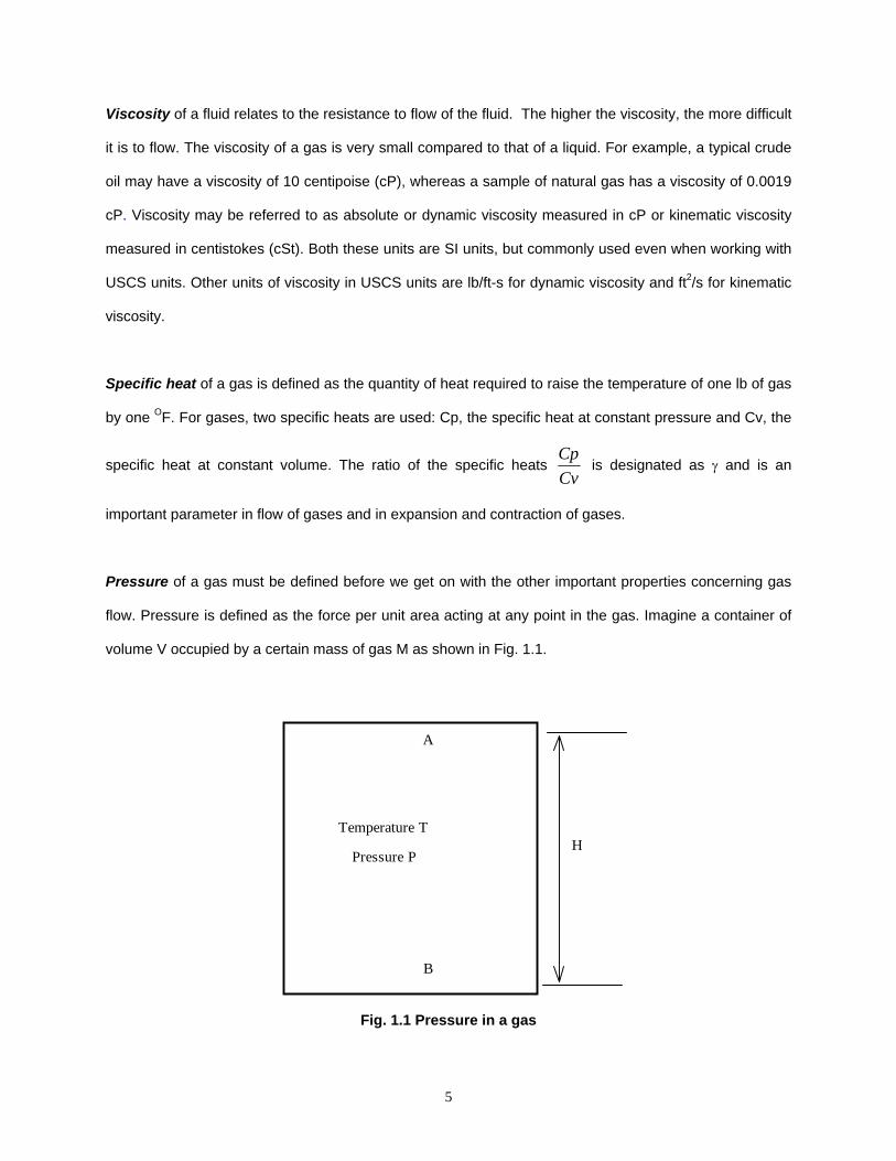
Pressure of a gas must be defined before we get on with the other important properties concerning gas

flow. Pressure is defined as the force per unit area acting at any point in the gas. Imagine a container of

volume V occupied by a certain mass of gas M as shown in Fig. 1.1.

Fig. 1.1 Pressure in a gas

B

A

HPressure P

Temperature T

6

The gas is contained within this volume at some temperature T and pressure P and is in equilibrium. At

every point within the container there is said to be a constant pressure P. Since the density of gas,

compared to that of a liquid, is very small, the pressure of the gas at a point A near the top of the

container will be the same as that at a point B near the bottom of the container. If the difference in

elevations between the two points is H, theoretically, the pressure of gas at the bottom point will be higher

than that at the top point by the additional weight of the column of gas of height H. However, since the

gas density is very small, this additional pressure is negligible. Therefore we say that the pressure of gas

is constant at every point within the container. In USCS units, gas pressure is expressed in lb/in2 or psi

and sometimes in lb/ft2 or psf. In SI units, pressure is stated as kilopascal (kPa), megapascal (MPa), bar

or kg/cm2. When dealing with gases it is very important to distinguish between gauge pressure and

absolute pressure. The absolute pressure at any point within the gas is the actual pressure inclusive of

the local atmospheric pressure (approximately 14.7 psi at sea level). Thus in the example above, if the

local atmospheric pressure outside the gas container is Patm and the gas pressure in the container as

measured by a pressure gauge is Pg, the absolute or total gas pressure in the container is:

Pabs = Pg + Patm (1.7)

The adder to the gauge pressure is also called the base pressure. In USCS units, the gauge pressure is

denoted by psig while the absolute pressure is stated as psia. Therefore, if the gauge pressure is 200

psig and the atmospheric pressure is 14.7 psi, the absolute pressure of the gas is 214.7 psia. In most

equations involving flow of gases and the gas laws, absolute pressure is used. Similar to absolute

pressure, we also refer to the absolute temperature of gas. The latter is obtained by adding a constant to

the gas temperature. For example, in USCS units, the absolute temperature scale is the Rankin scale. In

SI units, Kelvin is the absolute scale for temperature. The temperature in OF or OC can be converted to

absolute units as follows:

OR = OF + 460 (1.8)

K = OC + 273 (1.9)

Note that degrees Rankin is denoted by OR whereas for degrees Kelvin, the degree symbol is dropped.

Thus it is common to refer to the absolute temperature of a gas at 80 OF as (80 + 460) = 540 OR and if the

7

gas was at 20 OC, the corresponding absolute temperature will be (20 + 273) = 293 K. In most

calculations involving gas properties and gas flow, the absolute temperature is used.

The Compressibility factor, Z is a dimensionless parameter less than 1.00 that represents the deviation of

a real gas from an ideal gas. Hence it is also referred to as the gas deviation factor. At low pressures

and temperatures Z is nearly equal to 1.00 whereas at higher pressures and temperatures it may range

between 0.75 and 0.90. The actual value of Z at any temperature and pressure must be calculated taking

into account the composition of the gas and its critical temperature and pressure. Several graphical and

analytical methods are available to calculate Z. Among these, the Standing-Katz, AGA and CNGA

methods are quite popular. The critical temperature and the critical pressure of a gas are important

parameters that affect the compressibility factor and are defined as follows.

The critical temperature of a pure gas is that temperature above which the gas cannot be compressed

into a liquid, regardless of the pressure. The critical pressure is the minimum pressure required at the

critical temperature of the gas to compress it into a liquid.

As an example, consider pure methane gas with a critical temperature of 343 OR and critical pressure of

666 psia. The reduced temperature of a gas is defined as the ratio of the gas temperature to its critical

temperature, both being expressed in absolute units (OR or K). It is therefore a dimensionless number.

Similarly, the reduced pressure is a dimensionless number defined as the ratio of the absolute pressure

of gas to its critical pressure. Therefore we can state the following:

c

r TTT = (1.10)

c

r PPP = (1.11)

where:

P = pressure of gas, psia

8

T = temperature of gas, OR

Tr = reduced temperature, dimensionless

Pr = reduced pressure, dimensionless

Tc = critical temperature, OR

Pc = critical pressure, psia

Using the preceding equations, the reduced temperature and reduced pressure of a sample of methane

gas at 70OF and 1200 psia pressure can be calculated as follows:

5452.1343

46070=

+=rT

and

8018.1666

1200==rP

For natural gas mixtures, the terms pseudo-critical temperature and pseudo-critical pressure are used.

The calculation methodology will be explained shortly. Similarly we can calculate the pseudo-reduced

temperature and pseudo-reduced pressure of a natural gas mixture, knowing its pseudo-critical

temperature and pseudo-critical pressure.

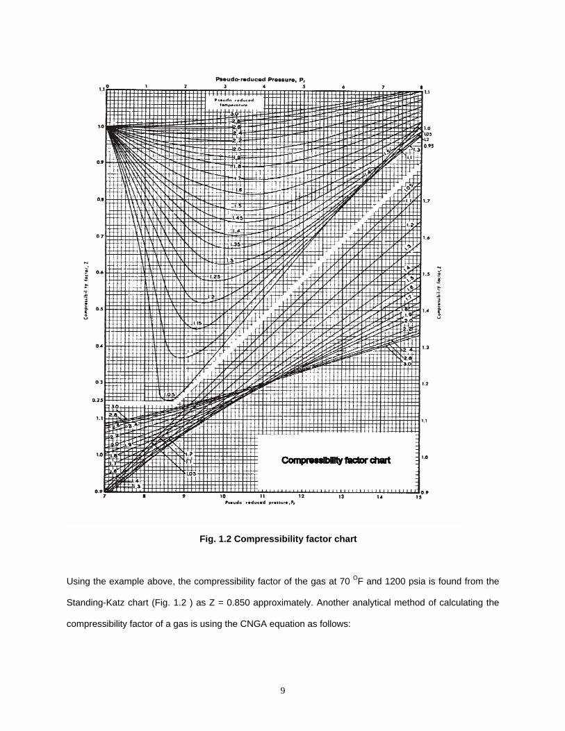
The Standing-Katz chart (Fig. 1.2_ can be used to determine the compressibility factor of a gas at any

temperature and pressure, once the reduced pressure and temperature are calculated knowing the

critical properties.

9

Fig. 1.2 Compressibility factor chart

Using the example above, the compressibility factor of the gas at 70 OF and 1200 psia is found from the

Standing-Katz chart (Fig. 1.2 ) as Z = 0.850 approximately. Another analytical method of calculating the

compressibility factor of a gas is using the CNGA equation as follows:

10

( )

⎥⎥⎦

⎤

⎢⎢⎣

⎡

⎟⎟⎠

⎞⎜⎜⎝

⎛+

=

825.3

785.1103444001

1

f

Gavg

TP

Z (1.12)

where:

Pavg = Gas pressure, psig.

Tf = Gas temperature, OR

G = Gas gravity (air = 1.00)

The CNGA equation for compressibility factor is valid when the average gas pressure Pavg is greater than

100 psig. For pressures less than 100 psig, compressibility factor is taken as 1.00. It must be noted that

the pressure used in the CNGA equation is the gauge pressure, not the absolute pressure.

Example 1

Calculate the compressibility factor of a sample of natural gas (gravity = 0.6) at 80 OF and 1000 psig using

the CNGA equation.

Solution

From the Eq. (1.12), the compressibility factor is:

( )⎥⎥⎦

⎤

⎢⎢⎣

⎡⎟⎟⎠

⎞⎜⎜⎝

⎛

+×

+

=×

825.3

6.0785.1

)46080(1034440010001

1Z = 0.8746

The CNGA method of calculating the compressibility, though approximate, is accurate enough for most

gas pipeline hydraulics work.

The heating value of a gas is expressed in Btu/ft3. It represents the quantity of heat in Btu (British

Thermal Unit) generated by the complete combustion of one cubic foot of the gas with air at constant

pressure and a fixed temperature of 60 OF. Two values of the heating value of a gas are used: Gross

heating value and Net heating value. The gross heating value is also called the higher heating value

11

(HHV) and the net heating value is called the lower heating value (LHV). The difference in the two values

represents the latent heat of vaporization of the water at standard temperature when complete

combustion of the gas occurs.

Natural gas mixtures

Natural gas generally consists of a mixture of several hydrocarbons, such as methane, ethane, etc.

Methane is the predominant component in natural gas. Sometimes small amounts of non-hydrocarbon

elements, such as nitrogen (N2), carbon-dioxide (CO2) and hydrogen sulfide (H2S) are also found. The

properties of a natural gas mixture can be calculated from the corresponding properties of the

components in the mixture. Kay’s rule is generally used to calculate the properties of a gas mixture, and

will be explained next.

Example 2

A natural gas mixture consists of the following components:

Component Percent Molecular weight

Methane C1 85 16.01

Ethane C2 10 30.07

Propane C3 5 44.10

________

Total 100

Calculate the specific gravity of this natural gas mixture.

Solution

Using Kay’s rule for a gas mixture, we can calculate the average molecular weight of the gas from the

component molecular weights given. By dividing the molecular weight by the molecular weight of air, we

can determine the specific gravity of the gas mixture. The average molecular weight per Kay’s rule is

calculated using a weighted average:

( ) ( ) ( ) 846.1810.4405.007.3010.004.1685.0 =×+×+×=M

12

Therefore, the specific gravity of the gas mixture is using Eq. (1.6):

6499.029846.18

==G

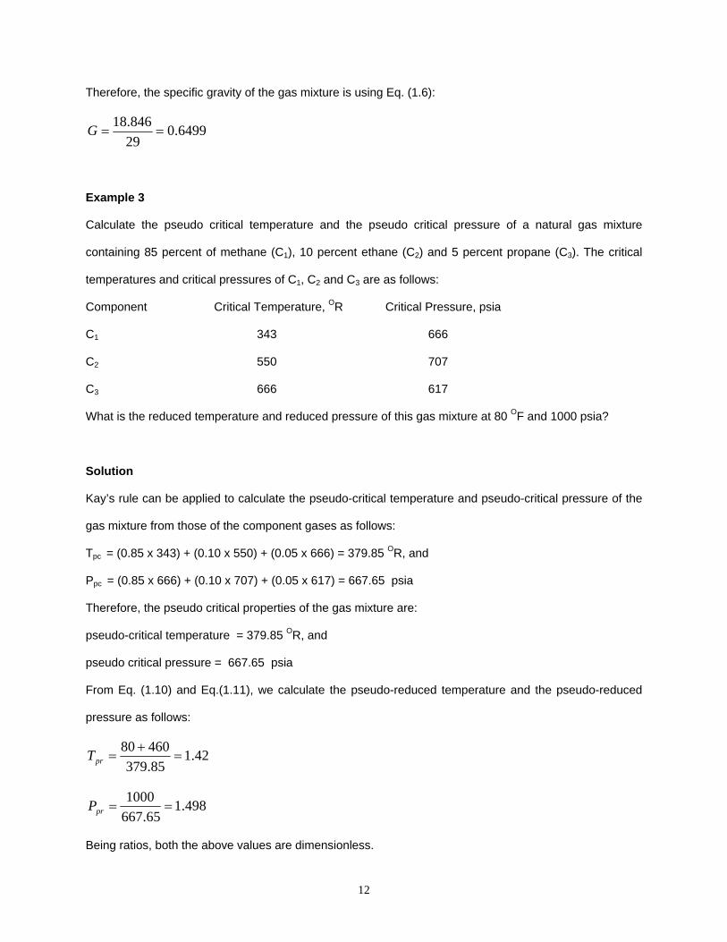
Example 3

Calculate the pseudo critical temperature and the pseudo critical pressure of a natural gas mixture

containing 85 percent of methane (C1), 10 percent ethane (C2) and 5 percent propane (C3). The critical

temperatures and critical pressures of C1, C2 and C3 are as follows:

Component Critical Temperature, OR Critical Pressure, psia

C1 343 666

C2 550 707

C3 666 617

What is the reduced temperature and reduced pressure of this gas mixture at 80 OF and 1000 psia?

Solution

Kay’s rule can be applied to calculate the pseudo-critical temperature and pseudo-critical pressure of the

gas mixture from those of the component gases as follows:

Tpc = (0.85 x 343) + (0.10 x 550) + (0.05 x 666) = 379.85 OR, and

Ppc = (0.85 x 666) + (0.10 x 707) + (0.05 x 617) = 667.65 psia

Therefore, the pseudo critical properties of the gas mixture are:

pseudo-critical temperature = 379.85 OR, and

pseudo critical pressure = 667.65 psia

From Eq. (1.10) and Eq.(1.11), we calculate the pseudo-reduced temperature and the pseudo-reduced

pressure as follows:

42.185.37946080

=+

=prT

498.165.667

1000==prP

Being ratios, both the above values are dimensionless.

13

If the gas composition is not known, the pseudo-critical properties may be calculated approximately from

the gas gravity as follows:

GTpc 344.307491.170 += (1.13)

GPpc 718.58604.709 −= (1.14)

where G is the gas gravity and other symbols are defined before.

Example 4

Calculate the pseudo critical temperature and pseudo critical pressure for a natural gas mixture

containing 85 percent methane, 10 percent ethane and 5 percent propane, using the approximate

method.

Solution

In Example 2, we calculated the gas gravity for this mixture as 0.6499. Using Eq. (1.13) and (1.14) the

pseudo critical properties are calculated as follows:

Tpc = 170.491 + 307.344 x (0.6499) = 370.23 OR

Ppc = 709.604 - 58.718 x (0.6499) = 671.44 psia

In a previous example, we calculated the pseudo-critical properties using the more accurate method as

379.85 OR and 667.65 psia. Comparing these with the approximate method using the gas gravity, we find

that the values are within 2.5 percent for the pseudo critical temperature and within 0.6 percent for the

pseudo critical pressure.

Gas Laws

The compressibility of a gas was introduced earlier and we defined it as a dimensionless number close to

1.0 that also represents how far a real gas deviates from an ideal gas. Ideal gases or perfect gases obey

Boyles and Charles law and have pressure, temperature and volume related by the ideal gas equation.

These laws for ideal gases are as follows:

14

Boyles Law defines the variation of pressure of a given mass of gas with its volume when the temperature

is held constant. The relationship between pressure P and volume V is

PV = constant (1.15)

Or

P1V1 = P2V2 (1.16)

where P1, V1 are the initial conditions and P2, V2 are the final conditions of a gas when temperature is

held constant. This is also called isothermal conditions.

Boyles law applies only when the gas temperature is constant. Thus if a given mass of gas has an initial

pressure of 100 psia and a volume of 10 ft3, with the temperature remaining constant at 80 OF and the

pressure increases to 200 psia, the corresponding volume of gas becomes:

Final volume = =×

20010100

5 ft3

Charles law applies to variations in pressure-temperature and volume-temperature, when the volume and

pressures are held constant. Thus keeping the volume constant, the pressure versus temperature

relationship according to Charles law is as follows:

=TP

constant (1.17)

Or

2

2

1

1

TP

TP

= (1.18)

Similarly if the pressure is held constant, the volume varies directly as the temperature as follows:

=TV

constant (1.19)

Or

2

2

1

1

TV

TV

= (1.20)

15

where P1, V1 and T1 are the initial conditions and P2, V2 and T2 are the final conditions. It must be noted

that pressures and temperatures must be in absolute units.

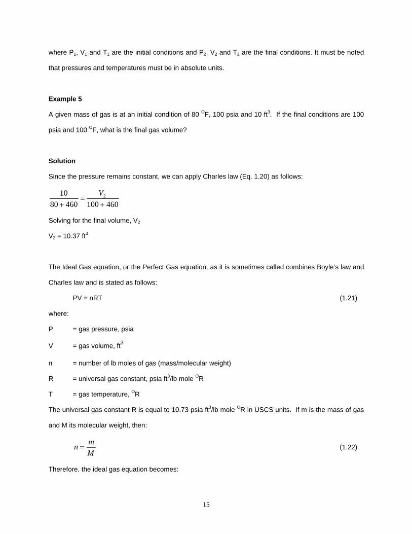
Example 5

A given mass of gas is at an initial condition of 80 OF, 100 psia and 10 ft3. If the final conditions are 100

psia and 100 OF, what is the final gas volume?

Solution

Since the pressure remains constant, we can apply Charles law (Eq. 1.20) as follows:

4601004608010 2

+=

+V

Solving for the final volume, V2

V2 = 10.37 ft3

The Ideal Gas equation, or the Perfect Gas equation, as it is sometimes called combines Boyle’s law and

Charles law and is stated as follows:

PV = nRT (1.21)

where:

P = gas pressure, psia

V = gas volume, ft3

n = number of lb moles of gas (mass/molecular weight)

R = universal gas constant, psia ft3/lb mole OR

T = gas temperature, OR

The universal gas constant R is equal to 10.73 psia ft3/lb mole OR in USCS units. If m is the mass of gas

and M its molecular weight, then:

Mmn = (1.22)

Therefore, the ideal gas equation becomes:

16

M

mRTPV = (1.23)

The constant R is the same for all ideal gases and therefore it is referred to as the universal gas constant.

The ideal gas equation discussed above is accurate only at low pressures. Because, in practice most

gas pipelines operate at pressures higher than atmospheric pressures, the ideal gas equation must be

modified when applied to real gases by including the effect of gas compressibility. Thus, when applied

to real gases, the compressibility factor or gas deviation factor is used in Eq. (1.21) as follows:

PV = ZnRT (1.24)

where Z is the gas compressibility factor at the given pressure and temperature.

Example 6

Calculate the volume of a 10 lb mass of gas (Gravity = 0.6) at 500 psig and 80 OF, assuming the

compressibility factor as 0.895. The molecular weight of air may be taken as 29 and the base pressure is

14.7 psia.

Solution

The number of lb moles n is calculated using Eq. (1.22). The molecular weight of the gas:

M = 0.6 x 29 = 17.4

Therefore, 5747.04.17

10==n lb mole

Using the real gas Eq. (1.24):

(500 + 14.7) V = 0.895 x 0.5747 x 10.73 x (80 + 460)

Therefore, V = 5.79 ft3

17

2. Pressure Drop Due To Friction

The Bernoulli’s equation essentially states the principle of conservation of energy. In a flowing fluid (gas

or liquid) the total energy of the fluid remains constant. The various components of the fluid energy are

transformed from one form to another, but no energy is lost as the fluid flows in a pipeline. Consider an

upstream location A and downstream location B in a pipe transporting a gas, at a flow rate of Q as shown

in Fig. 2.1

Fig 2.1 Energy of gas in pipe flow

At point A, the gas has a certain pressure PA, density ρ A, and temperature T A. Also the elevation of point

A above a certain datum is Z A. Similarly, the corresponding values for the downstream location B are P B,

ρ B, TB and ZB. If the pressures and elevations at A and B were the same, there would be no “driving

force” and hence no gas flow. Due to the difference in pressures and elevations, gas flows from point A

to point B. The reason for the pressure difference in a flowing gas is partly due to the elevation difference

and more due to the friction between the flowing gas and the pipe wall. As the internal roughness of the

pipe increases the friction increases. The velocity of the gas, which is proportional to the volume flow rate

Elevation Datum

ΖΒ

Pressure PA

A

B

ΖΑ

Pressure PB

Flow Q

Velocity VA

Velocity VB

density ρB

density ρA

18

Q, also changes depending upon the cross sectional area of the pipe and the pressures and temperature

of the gas. By the principle of conservation of mass, the same mass of gas flows at A as it does at B, if no

volumes of gas are taken out or introduced into the pipe between points A and B. Therefore, if VA and VB

represent the gas velocities at points A and B, we can state the following for the principle of conservation

of mass.

Mass flow = AAVAρA = ABVBρB (2.1)

In the above equation the product of the area A and Velocity V represents the volume flow rate, and by

multiplying the result by the density ρ, we get the mass flow rate at any cross section of the pipe. If the

pipe cross section is the same throughout (constant diameter pipeline), the mass flow equation reduces

to:

VAρA = VBρB (2.2)

Referring to Fig 2.1, for the flow of gas in a pipeline, the energy of a unit mass of gas at A may be

represented by the following three components:

Pressure energy A

APρ

(2.3)

Kinetic energy g

VA

2

2

(2.4)

Potential energy Z A (2.5)

All energy components have been converted to units of fluid head in feet and g is the acceleration due to

gravity. Its value at sea level is 32.2 ft/s2 in USCS units and 9.81 m/s2 in SI units.

If the frictional energy loss (in ft of head) in the pipeline from point A to point B is hf, we can write the

energy conservation equation or the Bernoulli’s equation as follows:

fBB

B

BA

A

A

A hZg

VPZg

VP+++=++

22

22

ρρ (2.6)

19

The term hf is also called the pressure loss due to friction between points A and B. Starting with the

Bernoulli’s equation, researchers have developed a formula for calculating the pressure drop in a gas

pipeline, taking into account the pipe diameter, length, elevations along the pipe, gas flow rate and the

gravity and compressibility of the gas. This basic equation is referred to the Fundamental Flow Equation,

also known as the General Flow equation.

As gas flows through a pipeline, its pressure decreases and the gas expands. In addition to the gas

properties, such as gravity and viscosity, the pipe inside diameter and pipe internal roughness influence

the pressure versus flow rate. Since the volume flow rate Q can vary with the gas pressure and

temperature, we must refer to some standard volume flow rate, based on standard conditions, such as 60

OF and 14.7 psia pressure. Thus the gas flow rate Q will be referred to as standard ft3/day or SCFD.

Variations of this are million standard ft3/day or MMSCFD and standard ft3/h or SCFH. In SI units, the gas

flow rate in a pipeline is stated in standard m3/hr or standard m3/day.

Pressure P1

Length L

Pressure P2Flow Q

1 2

Elevation H1Elevation H2

D

Fig 2.2 Steady state flow in a gas pipeline

Referring to Fig 2.2, for a pipe segment of length L and inside diameter D, the upstream pressure P1 and

the downstream pressure P2 are related to the flow rate and gas properties (based on USCS units) as

follows:

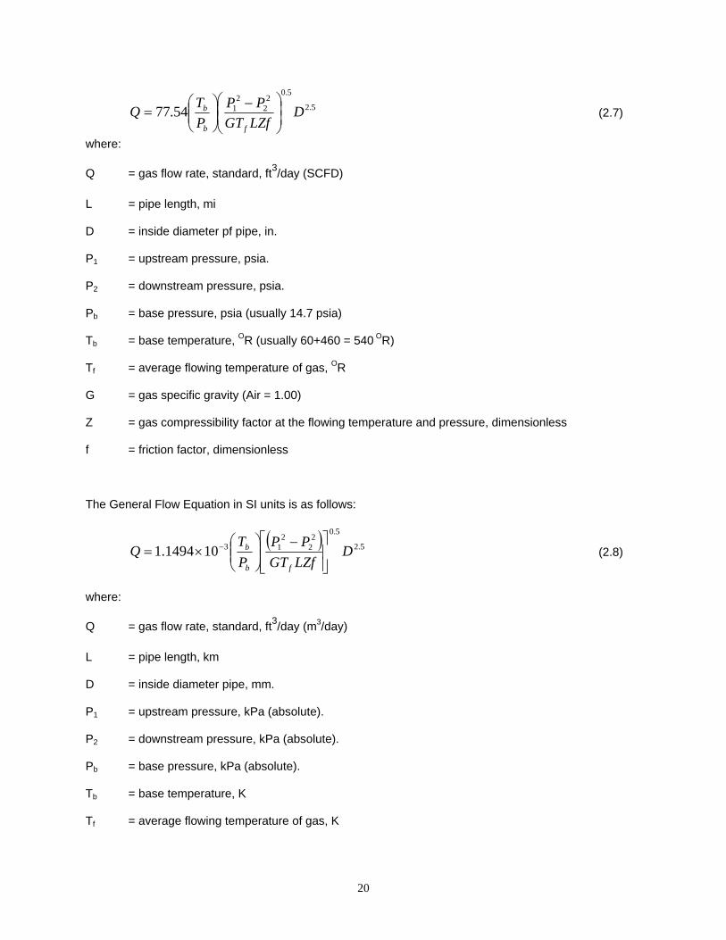
20

5.2

5.02

22

154.77 DLZfGTPP

PTQ

fb

b⎟⎟⎠

⎞⎜⎜⎝

⎛ −⎟⎟⎠

⎞⎜⎜⎝

⎛= (2.7)

where:

Q = gas flow rate, standard, ft3/day (SCFD)

L = pipe length, mi

D = inside diameter pf pipe, in.

P1 = upstream pressure, psia.

P2 = downstream pressure, psia.

Pb = base pressure, psia (usually 14.7 psia)

Tb = base temperature, OR (usually 60+460 = 540 OR)

Tf = average flowing temperature of gas, OR

G = gas specific gravity (Air = 1.00)

Z = gas compressibility factor at the flowing temperature and pressure, dimensionless

f = friction factor, dimensionless

The General Flow Equation in SI units is as follows:

( ) 5.2

5.02

22

13101494.1 DLZfGTPP

PT

Qfb

b

⎥⎥⎦

⎤

⎢⎢⎣

⎡ −⎟⎟⎠

⎞⎜⎜⎝

⎛×= − (2.8)

where:

Q = gas flow rate, standard, ft3/day (m3/day)

L = pipe length, km

D = inside diameter pipe, mm.

P1 = upstream pressure, kPa (absolute).

P2 = downstream pressure, kPa (absolute).

Pb = base pressure, kPa (absolute).

Tb = base temperature, K

Tf = average flowing temperature of gas, K

21

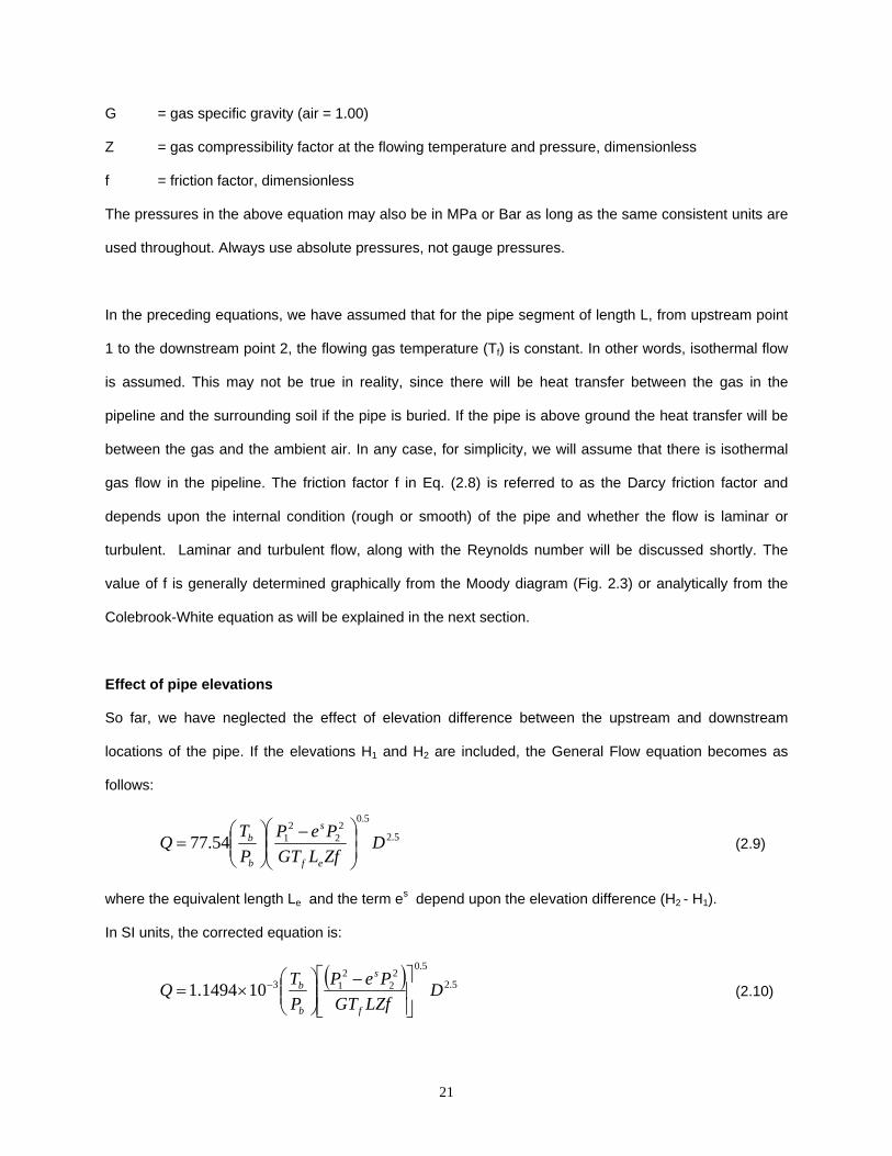
G = gas specific gravity (air = 1.00)

Z = gas compressibility factor at the flowing temperature and pressure, dimensionless

f = friction factor, dimensionless

The pressures in the above equation may also be in MPa or Bar as long as the same consistent units are

used throughout. Always use absolute pressures, not gauge pressures.

In the preceding equations, we have assumed that for the pipe segment of length L, from upstream point

1 to the downstream point 2, the flowing gas temperature (Tf) is constant. In other words, isothermal flow

is assumed. This may not be true in reality, since there will be heat transfer between the gas in the

pipeline and the surrounding soil if the pipe is buried. If the pipe is above ground the heat transfer will be

between the gas and the ambient air. In any case, for simplicity, we will assume that there is isothermal

gas flow in the pipeline. The friction factor f in Eq. (2.8) is referred to as the Darcy friction factor and

depends upon the internal condition (rough or smooth) of the pipe and whether the flow is laminar or

turbulent. Laminar and turbulent flow, along with the Reynolds number will be discussed shortly. The

value of f is generally determined graphically from the Moody diagram (Fig. 2.3) or analytically from the

Colebrook-White equation as will be explained in the next section.

Effect of pipe elevations

So far, we have neglected the effect of elevation difference between the upstream and downstream

locations of the pipe. If the elevations H1 and H2 are included, the General Flow equation becomes as

follows:

5.2

5.02

22

154.77 DZfLGTPeP

PTQ

ef

s

b

b⎟⎟⎠

⎞⎜⎜⎝

⎛ −⎟⎟⎠

⎞⎜⎜⎝

⎛= (2.9)

where the equivalent length Le and the term es depend upon the elevation difference (H2 - H1).

In SI units, the corrected equation is:

( ) 5.2

5.02

22

13101494.1 DLZfGT

PePPTQ

f

s

b

b

⎥⎥⎦

⎤

⎢⎢⎣

⎡ −⎟⎟⎠

⎞⎜⎜⎝

⎛×= − (2.10)

22

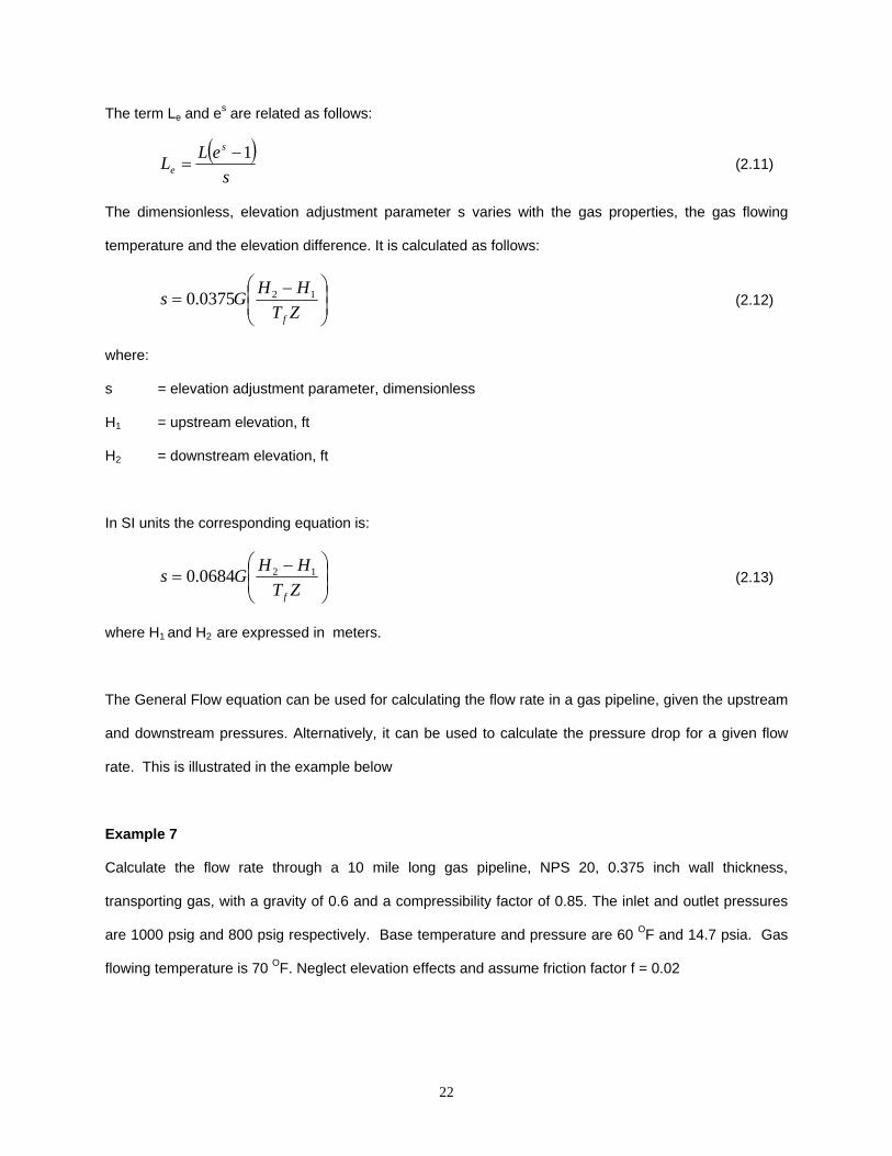
The term Le and es are related as follows:

( )

seLL

s

e1−

= (2.11)

The dimensionless, elevation adjustment parameter s varies with the gas properties, the gas flowing

temperature and the elevation difference. It is calculated as follows:

⎟⎟⎠

⎞⎜⎜⎝

⎛ −=

ZTHHGs

f

120375.0 (2.12)

where:

s = elevation adjustment parameter, dimensionless

H1 = upstream elevation, ft

H2 = downstream elevation, ft

In SI units the corresponding equation is:

⎟⎟⎠

⎞⎜⎜⎝

⎛ −=

ZTHHGs

f

120684.0 (2.13)

where H1 and H2 are expressed in meters.

The General Flow equation can be used for calculating the flow rate in a gas pipeline, given the upstream

and downstream pressures. Alternatively, it can be used to calculate the pressure drop for a given flow

rate. This is illustrated in the example below

Example 7

Calculate the flow rate through a 10 mile long gas pipeline, NPS 20, 0.375 inch wall thickness,

transporting gas, with a gravity of 0.6 and a compressibility factor of 0.85. The inlet and outlet pressures

are 1000 psig and 800 psig respectively. Base temperature and pressure are 60 OF and 14.7 psia. Gas

flowing temperature is 70 OF. Neglect elevation effects and assume friction factor f = 0.02

23

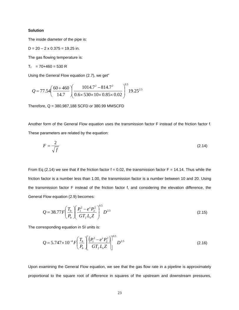
Solution

The inside diameter of the pipe is:

D = 20 – 2 x 0.375 = 19.25 in.

The gas flowing temperature is:

Tf = 70+460 = 530 R

Using the General Flow equation (2.7), we get”

5.2

5.022

25.1902.085.0105306.0

7.8147.10147.144606054.77 ⎟

⎟⎠

⎞⎜⎜⎝

⎛

××××

−⎟⎠⎞

⎜⎝⎛ +

=Q

Therefore, Q = 380,987,188 SCFD or 380.99 MMSCFD

Another form of the General Flow equation uses the transmission factor F instead of the friction factor f.

These parameters are related by the equation:

f

F 2= (2.14)

From Eq (2.14) we see that if the friction factor f = 0.02, the transmission factor F = 14.14. Thus while the

friction factor is a number less than 1.00, the transmission factor is a number between 10 and 20. Using

the transmission factor F instead of the friction factor f, and considering the elevation difference, the

General Flow equation (2.9) becomes:

5.2

5.02

22

177.38 DZLGTPeP

PTFQ

ef

s

b

b⎟⎟⎠

⎞⎜⎜⎝

⎛ −⎟⎟⎠

⎞⎜⎜⎝

⎛= (2.15)

The corresponding equation in SI units is:

( ) 5.2

5.02

22

1410747.5 DZLGTPeP

PTFQ

ef

s

b

b

⎥⎥⎦

⎤

⎢⎢⎣

⎡ −⎟⎟⎠

⎞⎜⎜⎝

⎛×= − (2.16)

Upon examining the General Flow equation, we see that the gas flow rate in a pipeline is approximately

proportional to the square root of difference in squares of the upstream and downstream pressures,

24

or ( )22

21 PP − . In comparison, in liquid flow through pipes, the flow rate is directly proportional to the

square root of the pressure difference or ( )21 PP − . This is a very important feature of gas flow in

pipes. The result of this is that the pressure gradient in a gas pipeline is slightly curved, compared to a

straight line in liquid flow. Also in a gas pipeline, reduction in upstream or downstream pressure at the

same flow rate will not be reflected to the same extent throughout the pipeline, unlike liquid flow.

Suppose the upstream pressure and downstream pressures are 1000 and 800 psia, respectively, at a

certain flow rate in a gas pipeline. By keeping the flow rate the same, a 100 psia reduction in upstream

pressure will not result in exactly 100 psia reduction in the downstream pressure, due to the Q versus

( )22

21 PP − relationship in gas flow. In a liquid pipeline, on the other hand, a 100 psia reduction in

upstream pressure will result in exactly 100 psia reduction in the downstream pressure.

Other interesting observations from the General Flow equation are as follows. The higher the gas gravity

and compressibility factor, the lower will be the flow rate, other items remaining the same. Similarly, the

longer the pipe segment, the lower will be the gas flow rate. Obviously, the larger the pipe diameter, the

greater will be the flow rate. Hotter gas flowing temperature causes reduction in flow rate. This is in stark

contrast to liquid flow in pipes where the higher temperature causes reduction in the liquid gravity and

viscosity, and hence increase the flow rate for a given pressure drop. In gas flow, we find that cooler

temperatures cause increase in flow rate. Thus summer flow rates are lower than winter flow rates in gas

pipelines.

Several other flow equations or pressure drop formulas for gas flow in pipes are commonly used. Among

these Panhandle A, Panhandle B and Weymouth equations have found their place in the gas pipeline

industry. The General Flow equation however is the most popular one and the friction factor f is

calculated by either using the Colebrook equation or the AGA formulas. Before we discuss the other flow

equations, we will review the different types of flows, Reynolds number and how the friction factor is

calculated using the Colebrook-White equation or the AGA method.

25

The flow through a pipeline may be classified as laminar, turbulent or critical flow depending upon the

value of a dimensionless parameter called the Reynolds number. The Reynolds number depends upon

the gas properties, pipe diameter and flow velocity and is defined as follows:

µ

ρVD=Re (2.17)

where: Re = Reynolds number, dimensionless V = average gas velocity, ft/s

D = pipe inside diameter, ft

ρ = gas density, lb/ft3 µ = gas viscosity, lb/ft-s In terms of the more commonly used units in the gas pipeline industry, the following formula for Reynolds

number is more appropriate, in USCS units:

⎟⎟⎠

⎞⎜⎜⎝

⎛⎟⎟⎠

⎞⎜⎜⎝

⎛=

DGQ

TP

b

b

µ0004778.0Re (2.18)

where: Pb = base pressure, psia

Tb = base temperature, OR

G = gas specific gravity

Q = gas flow rate, standard ft3/day (SCFD)

D = pipe inside diameter, in.

µ = gas viscosity, lb/ft-s

The corresponding version in SI units is as follows:

⎟⎟⎠

⎞⎜⎜⎝

⎛⎟⎟⎠

⎞⎜⎜⎝

⎛=

DGQ

TP

b

b

µ5134.0Re (2.19)

where:

26

Pb = base pressure, kPa

Tb = base temperature, K

G = gas specific gravity

Q = gas flow rate, standard m3/day

D = pipe inside diameter, mm

µ = gas viscosity, Poise

The flow in a gas pipeline is considered to be laminar flow when the Reynolds number is below 2000.

Turbulent flow is said to exist when the Reynolds number is greater than 4000. When the Reynolds

numbers is between 2000 and 4000, the flow is called critical flow, or undefined flow.

Therefore,

Re <= 2000 Flow is laminar

Re > 4000 Flow is turbulent

And Re > 2000 and Re <= 4000 Flow is critical flow

In practice, most gas pipelines operate at flow rates that produce high Reynolds numbers, and therefore

in the turbulent flow regime. Actually, the turbulent flow regime is further divided into three regions known

as smooth pipe flow, fully rough pipe flow and transition flow. This is illustrated in the Moody diagram

shown in Fig 2.3 below.

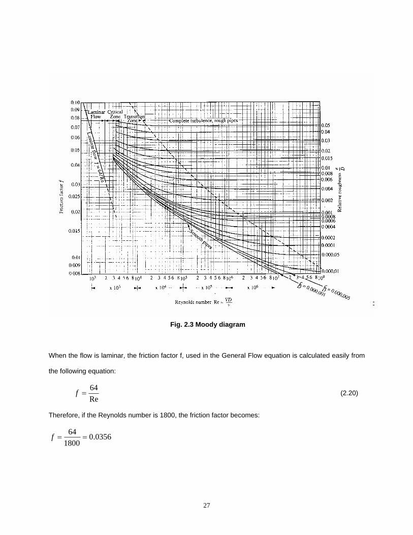
27

Fig. 2.3 Moody diagram

When the flow is laminar, the friction factor f, used in the General Flow equation is calculated easily from

the following equation:

Re64

=f (2.20)

Therefore, if the Reynolds number is 1800, the friction factor becomes:

0356.01800

64==f

28

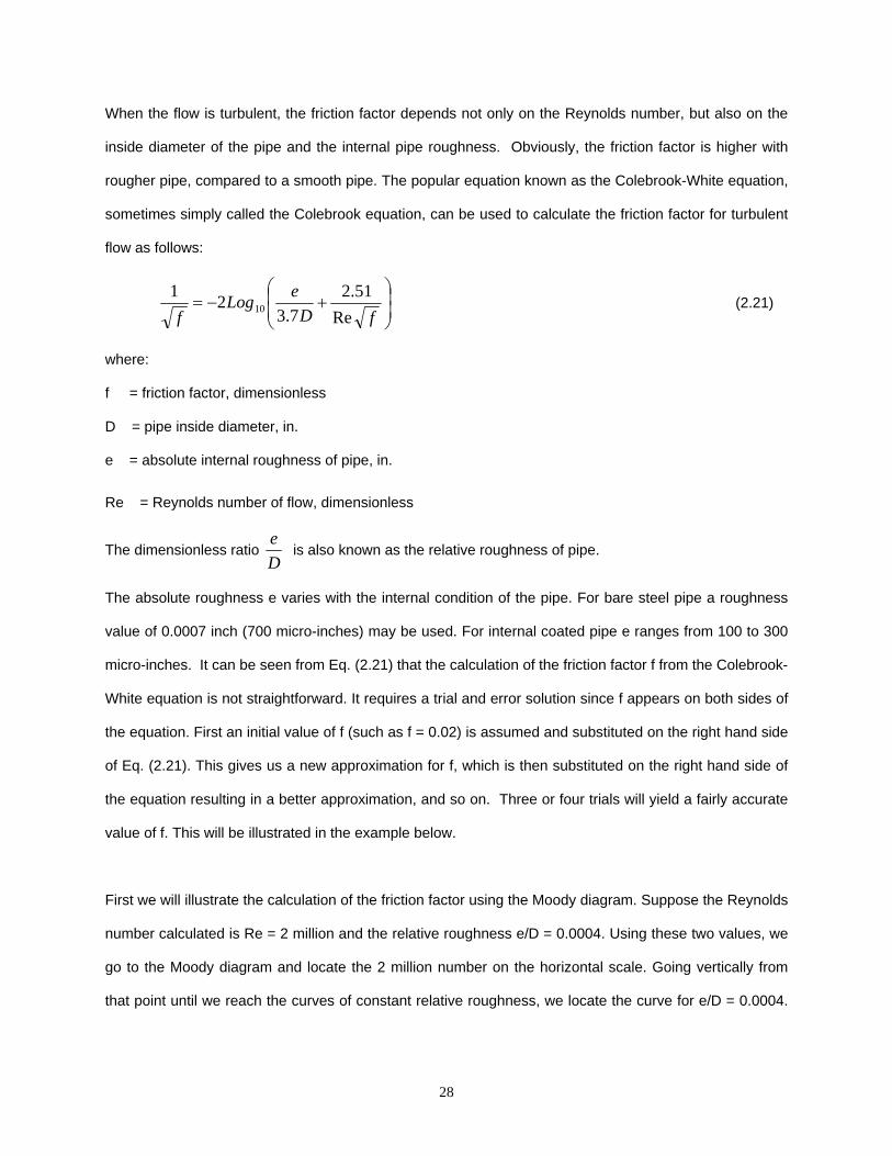
When the flow is turbulent, the friction factor depends not only on the Reynolds number, but also on the

inside diameter of the pipe and the internal pipe roughness. Obviously, the friction factor is higher with

rougher pipe, compared to a smooth pipe. The popular equation known as the Colebrook-White equation,

sometimes simply called the Colebrook equation, can be used to calculate the friction factor for turbulent

flow as follows:

⎟⎟⎠

⎞⎜⎜⎝

⎛+−=

fDeLog

f Re51.2

7.321

10 (2.21)

where:

f = friction factor, dimensionless

D = pipe inside diameter, in.

e = absolute internal roughness of pipe, in.

Re = Reynolds number of flow, dimensionless

The dimensionless ratio De

is also known as the relative roughness of pipe.

The absolute roughness e varies with the internal condition of the pipe. For bare steel pipe a roughness

value of 0.0007 inch (700 micro-inches) may be used. For internal coated pipe e ranges from 100 to 300

micro-inches. It can be seen from Eq. (2.21) that the calculation of the friction factor f from the Colebrook-

White equation is not straightforward. It requires a trial and error solution since f appears on both sides of

the equation. First an initial value of f (such as f = 0.02) is assumed and substituted on the right hand side

of Eq. (2.21). This gives us a new approximation for f, which is then substituted on the right hand side of

the equation resulting in a better approximation, and so on. Three or four trials will yield a fairly accurate

value of f. This will be illustrated in the example below.

First we will illustrate the calculation of the friction factor using the Moody diagram. Suppose the Reynolds

number calculated is Re = 2 million and the relative roughness e/D = 0.0004. Using these two values, we

go to the Moody diagram and locate the 2 million number on the horizontal scale. Going vertically from

that point until we reach the curves of constant relative roughness, we locate the curve for e/D = 0.0004.

29

From the point of intersection, we go horizontally to the left and read the value of the friction factor f as f =

0.016.

In the next example, the calculation of f using the Colebrook equation will be explained.

Example 8

A gas pipeline, NPS 24 with 0.500 in. wall thickness transports 250 MMSCFD of natural gas having a

specific gravity of 0.65 and a viscosity of 0.000008 lb/ft-s. Calculate the value of Reynolds number and

the Colebrook-White friction factor, based on a pipe roughness of 700 micro-inches. The base

temperature and base pressure are 60 OF and 14.73 psia, respectively. What is the corresponding

transmission factor F?

Solution

Inside diameter of pipe = 24 – 2 x 0.5 = 23.0 in.

Base temperature = 60 + 460 = 520 OR

Using Eq. (2.18), the Reynolds number is:

⎟⎟⎠

⎞⎜⎜⎝

⎛×××

⎟⎠⎞

⎜⎝⎛=

23000008.01025065.0

52073.140004778.0Re

6

= 11,953,115

Therefore the flow is in the turbulent region.

From Eq. (2.21), we calculate the friction factor as follows:

Relative roughness = De

= 23

10700 6−× = 0.0000304

⎟⎟⎠

⎞⎜⎜⎝

⎛+−=

fLog

f 115,953,1151.2

7.30000304.021

10

First assume f = 0.02 and calculate a better approximation from above as:

⎟⎟⎠

⎞⎜⎜⎝

⎛+−=

02.0115,953,1151.2

7.30000304.021

10Logf

= 10.0264 or f = 0.0099

Therefore f = 0.0099 is a better approximation.

30

Next using this value, we get the next better approximation as:

⎟⎟⎠

⎞⎜⎜⎝

⎛+−=

0099.0115,953,1151.2

7.30000304.021

10Logf

Solving for f we get f = 0.0101. The next trial yields f = 0.0101, which is the same as the last calculated

value. Hence the solution for the friction factor is f = 0.0101. The corresponding transmission factor F is

calculated from Eq. (2.14) as:

95.190101.02

==F

Another popular correlation for the transmission factor (and hence the friction factor) is the AGA equation.

It is also referred to as the AGA NB-13 method. Using the AGA method, the transmission factor F is

calculated in two steps. First the transmission factor is calculated for the rough pipe law. Next F is

calculated based upon the smooth pipe law. These two zones refer to the Moody diagram discussed

earlier. The smaller of the two values calculated is the AGA transmission factor. This factor is then used

in the General Flow equation to calculate the pressure drop. The method of calculation is as follows:

Using the rough pipe law, AGA recommends the following formula for F for a given pipe diameter and

roughness. It is calculated independent of the Reynolds number.

⎟⎠⎞

⎜⎝⎛=

eDLogF 7.34 10 (2.22)

This calculation for the rough pipe regime is also called the Von Karman rough pipe flow equation.

Next, F is calculated for the partially turbulent zone using the following equations, taking into account the

Reynolds number, the pipe drag factor and the Von Karman smooth pipe transmission factor Ft.

⎟⎟⎠

⎞⎜⎜⎝

⎛=

tf FLogDF

4125.1Re4 10 (2.23)

and

31

6.0Re4 10 −⎟⎟⎠

⎞⎜⎜⎝

⎛=

tt F

LogF (2.24)

where:

Ft = Von Karman smooth pipe transmission factor

Df = pipe drag factor

The value of Ft must be calculated from Eq. (2.24) by trial and error. The pipe drag factor Df is a

dimensionless parameter that is a function of the Bend Index (BI) of the pipe. The bend index depends

upon the number of bends and fittings in the pipe. The BI is calculated by adding all the angles and bends

in the pipe segment, and dividing the total by the total length of the pipe segment. The drag factor Df

generally ranges between 0.90 and 0.99 and can be found from Table 1 below.

Table 1 – Bend Index and Drag Factor

Bend Index Extremely low Average Extremely high 5o to 10o 60o to 80o 200o to 300o Bare steel 0.975 - 0.973 0.960 - 0.956 0.930 - 0.900 Plastic lined 0.979 - 0.976 0.964 - 0.960 0.936 - 0.910 Pig Burnished 0.982 - 0.980 0.968 - 0.965 0.944 - 0.920 Sand-Blasted 0.985 - 0.983 0.976 - 0.970 0.951 - 0.930 Note: The drag factors above are based on 40 ft joints of pipelines and mainline valves at 10 mile spacing

Additional data on the bend index and drag factor may be found in the AGA NB-13 Committee Report. An

example using the AGA transmission factor will be illustrated in the example below.

Example 9 A natural gas pipeline NPS 24 with 0.500 in. wall thickness transport gas at 250 MMSCFD. Calculate the

AGA transmission factor and friction factor. The gas gravity and viscosity are 0.59 and 0.000008 lb/ft-sec,

respectively. Assume an absolute pipe roughness of 750 micro-inches and a bend index of 60O. Given

base pressure = 14.7 psia and base temperature = 60 OF.

32

Solution

Pipe inside diameter = 24 – 2 x 0.5 = 23.0 in.

Base temperature = 60 + 460 = 520 OR

First calculate the Reynolds number from Eq. (2.18):

=××

××××=

520000008.00.237.1459.0102500004778.0Re

6

10,827,653

Next we will calculate the transmission factor for the fully turbulent flow using the rough pipe law Eq.

(2.22):

⎟⎠⎞

⎜⎝⎛ ×

=00075.0

0.237.34 10LogF = 20.22

Next, for the smooth pipe zone, the Von Karman transmission factor is calculated from Eq. (2.24) as:

6.0653,827,104 10 −⎟⎟⎠

⎞⎜⎜⎝

⎛=

tt F

LogF

Solving for Ft by trial and error, Ft = 22.16.

The bend index of 60O gives a drag factor Df of 0.96, from Table 1.

Therefore, the transmission factor for the partially turbulent flow zone is from Eq. (2.23):

⎟⎠⎞

⎜⎝⎛

××=

16.224125.1653,827,1096.04 10LogF = 21.27

Therefore, choosing the smaller of the two values calculated above, the AGA transmission factor is:

F = 20.22

The corresponding friction factor f is found from Eq. (2.14):

22.202=

f

Therefore, f = 0.0098

Average pipeline pressure

The gas compressibility factor Z used in the General Flow equation is based upon the flowing

temperature and the average pipe pressure. The average pressure may be approximated as the

33

arithmetic average 2

21 PP + of the upstream and downstream pressures P1 and P2. However, a more

accurate average pipe pressure is usually calculated as follows:

⎟⎟⎠

⎞⎜⎜⎝

⎛+

−+=21

21213

2PP

PPPPPavg (2.25)

The preceding equation may also be written as:

⎟⎟⎠

⎞⎜⎜⎝

⎛

−−

= 22

21

32

31

32

PPPP

Pavg (2.26)

Since the pressures used in the General Flow equation are in absolute units, all gauge pressures must be

converted to absolute pressures, when calculating the average pressure from Eq. (2.25) and (2.26). As

an example, if the upstream and downstream pressures are 1200 psia and 1000 psia respectively, the

average pressure in the pipe segment is:

⎟⎠⎞

⎜⎝⎛ ×

−+=2200

100012001000120032

avgP = 1103.03 psia

If we used the arithmetic average, this becomes:

( )1000120021

+=avgP = 1100 psia

Velocity of gas in pipe flow The velocity of gas flow in a pipeline under steady state flow can be calculated by considering the volume

flow rate and pipe diameter. In a liquid pipeline, under steady flow, the average flow velocity remains

constant throughout the pipeline, as long as the inside diameter does not change. However, in a gas

pipeline, due to compressibility effects, pressure variation and temperature variation, the average gas

velocity will vary along the pipeline even if the pipe inside diameter remains the same. The average

velocity in a gas pipeline at any location along the pipeline is a function of the flow rate, gas

compressibility factor, pipe diameter, pressure and temperature, as indicated in the equation below:

34

⎟⎠⎞

⎜⎝⎛

⎟⎟⎠

⎞⎜⎜⎝

⎛⎟⎟⎠

⎞⎜⎜⎝

⎛= 2002122.0

DQ

PTZ

TPV b

b

b (2.27)

where:

V = Average gas velocity, ft/s

Qb = gas flow rate, standard ft3/day (SCFD)

D = inside diameter of pipe, in.

Pb = base pressure, psia

Tb = base temperature, OR

P = gas pressure, psia.

T = gas temperature, OR

Z = gas compressibility factor at pipeline conditions, dimensionless

It can be seen from the velocity equation that the higher the pressure, the lower the velocity and vice

versa. The corresponding equation for the velocity in SI units is as follows:

⎟⎠⎞

⎜⎝⎛

⎟⎠⎞

⎜⎝⎛

⎟⎟⎠

⎞⎜⎜⎝

⎛= 27349.14

DQ

PZT

TPV b

b

b (2.28)

where:

V = gas velocity, m/s

Qb = gas flow rate, standard m3/day

D = inside diameter of pipe, mm

Pb = base pressure, kPa

Tb = base temperature, K

P = gas pressure, kPa.

T = gas temperature, K

Z = gas compressibility factor at pipeline conditions, dimensionless

In the SI version of the equation, the pressures may be in any one consistent set of units, such as kPa,

MPa or Bar.

35

Erosional velocity

The erosional velocity represents the upper limit of gas velocity in a pipeline. As the gas velocity

increases, vibration and noise result. Higher velocities also cause erosion of the pipe wall over a long

time period. The erosional velocity Vmax may be calculated approximately as follows:

GPZRTV29

100max = (2.29)

where:

Z = gas compressibility factor, dimensionless

R = gas constant = 10.73 ft3 psia/lb-moleR

T = gas temperature, 0R

G = gas gravity (air = 1.00)

P = gas pressure, psia

Example 10

A natural gas pipeline NPS 20 with 0.500 in. wall thickness transports natural gas (specific gravity = 0.65)

at a flow rate of 200 MMSCFD at an inlet temperature of 70 OF. Calculate the gas velocity at inlet and

outlet of the pipe, assuming isothermal flow. The inlet pressure is 1200 psig and the outlet pressure is

900 psig. The base pressure is 14.7 psia and the base temperature is 60 OF. Use average compressibility

factor of 0.95. Also, calculate the erosional velocity for this pipeline.

Solution

From Eq. (2.27) the gas velocity at the pipe inlet pressure of 1200 psig is:

95.07.1214

46070460607.14

0.1910200002122.0 2

6

1 ×⎟⎠⎞

⎜⎝⎛ +

⎟⎠⎞

⎜⎝⎛

+⎟⎟⎠

⎞⎜⎜⎝

⎛ ×=V

= 13.78 ft/s

Similarly, the gas velocity at the outlet pressure of 900 psig can be calculated using proportions from Eq.

(2.27):

36

7.9147.121478.132 ×=V = 18.30 ft/s

Finally, the erosional velocity can be calculated using Eq. (2.29):

7.121465.02953073.1095.0100max ××

××=u = 48.57 ft/s

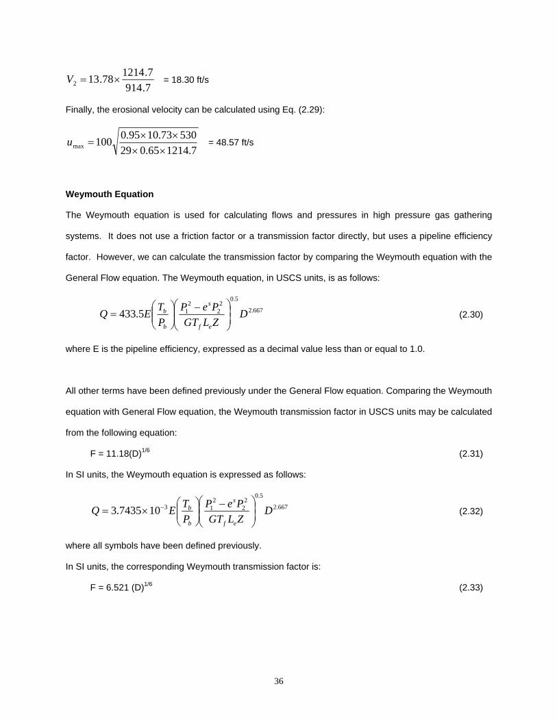
Weymouth Equation

The Weymouth equation is used for calculating flows and pressures in high pressure gas gathering

systems. It does not use a friction factor or a transmission factor directly, but uses a pipeline efficiency

factor. However, we can calculate the transmission factor by comparing the Weymouth equation with the

General Flow equation. The Weymouth equation, in USCS units, is as follows:

667.2

5.02

22

15.433 DZLGTPeP

PTEQ

ef

s

b

b⎟⎟⎠

⎞⎜⎜⎝

⎛ −⎟⎟⎠

⎞⎜⎜⎝

⎛= (2.30)

where E is the pipeline efficiency, expressed as a decimal value less than or equal to 1.0.

All other terms have been defined previously under the General Flow equation. Comparing the Weymouth

equation with General Flow equation, the Weymouth transmission factor in USCS units may be calculated

from the following equation:

F = 11.18(D)1/6 (2.31)

In SI units, the Weymouth equation is expressed as follows:

667.2

5.02

22

13107435.3 DZLGTPeP

PTEQ

ef

s

b

b⎟⎟⎠

⎞⎜⎜⎝

⎛ −⎟⎟⎠

⎞⎜⎜⎝

⎛×= − (2.32)

where all symbols have been defined previously.

In SI units, the corresponding Weymouth transmission factor is:

F = 6.521 (D)1/6 (2.33)

37

Panhandle Equations

The Panhandle A and the Panhandle B Equations have been used by many natural gas pipeline

companies, including a pipeline efficiency factor, instead of considering the pipe roughness. These

equations have been successfully used for Reynolds numbers in the range of 4 million to 40 million.

The more common versions of Panhandle A equation is as follows:

6182.2

5394.0

8539.0

22

21

0788.1

87.435 DZLTG

PePPTEQ

ef

s

b

b⎟⎟⎠

⎞⎜⎜⎝

⎛ −⎟⎟⎠

⎞⎜⎜⎝

⎛= (2.34)

where E is the pipeline efficiency, a decimal value less than 1.0, and all other symbols have been defined

before under General Flow equation.

In SI Units, the Panhandle A equation is stated as follows:

6182.2

5394.0

8539.0

22

21

0788.13105965.4 D

ZLTGPeP

PTEQ

ef

s

b

b⎟⎟⎠

⎞⎜⎜⎝

⎛ −⎟⎟⎠

⎞⎜⎜⎝

⎛×= − (2.35)

All symbols have been previously defined. It must be noted that in the preceding SI version, all pressures

are in kPa. If MPa or Bar is used, the constant in Eq.(2.35) will be different.

The Panhandle B equation, sometimes called the revised Panhandle equation, is used by many gas

transmission companies. It is found to be fairly accurate in turbulent flow for Reynolds numbers between

4 million and 40 million. It is expressed as follows, in USCS units:

53.2

51.0

961.0

22

21

02.1

737 DZLTG

PePPTEQ

ef

s

b

b⎟⎟⎠

⎞⎜⎜⎝

⎛ −⎟⎟⎠

⎞⎜⎜⎝

⎛= (2.36)

where all symbols are the same as defined for the Panhandle A equation (2.34).

The corresponding equation in SI units is as follows:

53.2

51.0

961.0

22

21

02.1210002.1 D

ZLTGPeP

PTEQ

ef

s

b

b⎟⎟⎠

⎞⎜⎜⎝

⎛ −⎟⎟⎠

⎞⎜⎜⎝

⎛×= − (2.37)

where all symbols are the same as defined for the Panhandle A equation (2.35).

38

Example 11 Calculate the outlet pressure in a natural gas pipeline, NPS 18 with 0.250 in. wall thickness, 20 miles

long, using Panhandle A and B equations. The gas flow rate is 150 MMSCFD at a flowing temperature of

70 OF. The inlet pressure is 1000 psig and the gas gravity and viscosity are 0.6 and 0.000008 lb/ft-sec,

respectively. Assume base pressure = 14.7 psia and base temperature = 60 OF. Assume that the

compressibility factor Z = 0.85 throughout and the pipeline efficiency is 0.95. Compare the results using

the Weymouth Equation. Neglect elevation effects.

Solution

Inside diameter D = 18 – 2 x 0.250 = 17.50 in

Gas flowing temperature Tf = 70 + 460 = 530 OR

Upstream pressure P1 = 1000 + 14.7 = 1014.7 psia

Base temperature Tb = 60 + 460 = 520 OR

Base pressure Pb = 14.7 psia

Using the Panhandle A Eq. (2.34), we get:

6182.2

5394.0

8539.0

22

20788.16 5.17

85.0205306.07.1014

7.1452095.087.43510150 ⎟

⎟⎠

⎞⎜⎜⎝

⎛

×××

−⎟⎠⎞

⎜⎝⎛×=×

P

Solving, P2 = 970.81 psia

Using the Panhandle B Eq. (2.36), we get:

53.2

51.0

961.0

22

202.16 5.17

85.0205306.07.1014

7.1452095.073710150 ⎟

⎟⎠

⎞⎜⎜⎝

⎛

×××

−⎟⎠⎞

⎜⎝⎛×=×

P

Solving for the outlet pressure P2, we get: P2 = 971.81 psia

Thus, both Panhandle A and B give results that are quite close. Next using the Weymouth Eq. (2.30) we get:

667.2

5.022

26 5.17

85.0205306.07.1014

7.1452095.05.43310150 ⎟

⎟⎠

⎞⎜⎜⎝

⎛

×××

−⎟⎠⎞

⎜⎝⎛×=×

P

Solving for the outlet pressure P2, we get:

39

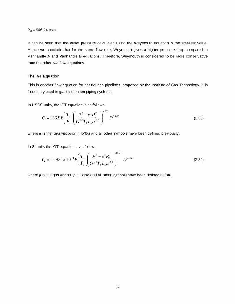
P2 = 946.24 psia

It can be seen that the outlet pressure calculated using the Weymouth equation is the smallest value.

Hence we conclude that for the same flow rate, Weymouth gives a higher pressure drop compared to

Panhandle A and Panhandle B equations. Therefore, Weymouth is considered to be more conservative

than the other two flow equations.

The IGT Equation

This is another flow equation for natural gas pipelines, proposed by the Institute of Gas Technology. It is

frequently used in gas distribution piping systems.

In USCS units, the IGT equation is as follows:

667.2

555.0

2.08.0

22

219.136 D

LTGPeP

PT

EQef

s

b

b⎟⎟⎠

⎞⎜⎜⎝

⎛ −⎟⎟⎠

⎞⎜⎜⎝

⎛=

µ (2.38)

where µ is the gas viscosity in lb/ft-s and all other symbols have been defined previously.

In SI units the IGT equation is as follows:

667.2

555.0

2.08.0

22

213102822.1 D

LTGPeP

PT

EQef

s

b

b⎟⎟⎠

⎞⎜⎜⎝

⎛ −⎟⎟⎠

⎞⎜⎜⎝

⎛×= −

µ (2.39)

where µ is the gas viscosity in Poise and all other symbols have been defined before.

40

3. Pressures and Piping System

In the previous sections we discussed how the pressure drop is related to the gas flow rate in a pipeline.

We calculated flow rates, for short pipe segments, from given upstream and downstream pressures using

the General Flow equation as well as Panhandle A, Panhandle B and Weymouth equations. In a long

pipeline, the pressures along the pipeline may be calculated considering the pipeline sub-divided into

short segments and by calculating the pressure drop in each segment. If we do not do this and consider

the pipeline as one long segment, the results will be inaccurate due to the nature of the relationship

between pressures and flow rates. To accurately calculate the pressures in a long gas pipeline, we have

to use some sort of a computer program, because subdividing the pipeline into segments and calculating

the pressures in each segment will become a laborious and time consuming process. Furthermore, if we

consider heat transfer effects, the calculations will be even more complex. We will illustrate the method of

calculating pressures by sub-dividing the pipeline, using a simple example. In this example we will first

calculate the pressures by considering the pipeline as one segment. Next we will sub-divide the pipeline

into two segments and repeat the calculations.

Example 12

A natural gas pipeline, AB is 100 mi long and is NPS16, 0.250 in. wall thickness. The elevation

differences may be neglected and the pipeline assumed to be along a flat elevation profile. The gas flow

rate is 100 MMSCFD. It is required to determine the pressure at the inlet A, considering a fixed delivery

pressure of 1000 psig at the terminus B. The gas gravity and viscosity are 0.6 and 0.000008 lb/ft-s,

respectively. The gas flowing temperature is 70 OF throughout. The base temperature and pressure are

60 OF and 14.7 psia respectively. Use CNGA method for calculating the compressibility factor. Assume

transmission factor F = 20.0 and use the General Flow equation for calculating the pressures.

Solution:

The inside diameter of the pipeline is:

D = 16-2x0.250 = 15.5 in.

41

For the compressibility factor, we need to know the gas temperature and the average pressure. Since we

do not know the upstream pressure at A, we cannot calculate an accurate average pressure. We will

assume that the average pressure is 1200 psig, since the pressure at B is 1000 psig. The approximate

compressibility factor will be calculated using this pressure from Eq. (1.12):

( )⎥⎥⎦

⎤

⎢⎢⎣

⎡⎟⎟⎠

⎞⎜⎜⎝

⎛ ××+

=×

825.3

6.0785.1

5301034440012001

1Z

Therefore, Z = 0.8440

This value can be adjusted after we calculate the actual pressures.

Using the General Flow equation, Eq. (2.7), considering the pipeline as one 100 mile long segment, the

pressure at the inlet A can be calculated as follows:

5.2

5.02216 5.15

844.01005306.07.1014

7.145202077.3810100 ⎟

⎟⎠

⎞⎜⎜⎝

⎛

×××

−⎟⎠⎞

⎜⎝⎛×=×

P

Solving for the pressure at A, we get:

P1 = 1195.14 psia or 1180.44 psig.

Based on this upstream pressure and the downstream pressure of 1000 psig at B, the average pressure

becomes, from Eq. (2.26):

⎟⎠⎞

⎜⎝⎛

+×

−+=7.101414.11957.101414.11957.101414.1195

32

avgP = 1107.38 psia or 1092.68 psig

This compares with the average pressure of 1200 psig we initially used to calculate Z. Therefore, a more

correct value of Z can be re-calculated using the average pressure calculation above. Strictly speaking

we must re-calculate Z based on the new average pressure of 1092.68 psig and then re-calculate the

pressure at A using the General Flow equation. The process must be repeated until successive values of

Z are within a small tolerance, such as 0.01. This is left as an exercise for the reader.

42

A B

NPS 16 pipeline 100 miles long

1000 psig

Flow

C

50 miles

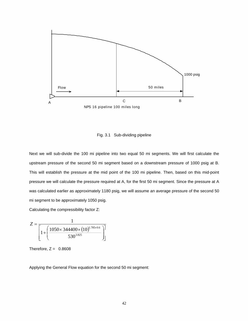
Fig. 3.1 Sub-dividing pipeline

Next we will sub-divide the 100 mi pipeline into two equal 50 mi segments. We will first calculate the

upstream pressure of the second 50 mi segment based on a downstream pressure of 1000 psig at B.

This will establish the pressure at the mid point of the 100 mi pipeline. Then, based on this mid-point

pressure we will calculate the pressure required at A, for the first 50 mi segment. Since the pressure at A

was calculated earlier as approximately 1180 psig, we will assume an average pressure of the second 50

mi segment to be approximately 1050 psig.

Calculating the compressibility factor Z:

( )⎥⎥⎦

⎤

⎢⎢⎣

⎡⎟⎟⎠

⎞⎜⎜⎝

⎛ ××+

=×

825.3

6.0785.1

5301034440010501

1Z

Therefore, Z = 0.8608

Applying the General Flow equation for the second 50 mi segment:

43

5.2

5.02216 5.15

8608.0505306.07.1014

7.145202077.3810100 ⎟

⎟⎠

⎞⎜⎜⎝

⎛

×××

−⎟⎠⎞

⎜⎝⎛×=×

P

Solving for the pressure at the mid point C, we get:

P1 = 1110.38 psia, or 1095.68 psig.

As before, the average gas pressure in the second segment must be calculated based on the above

pressure, the pressure at B, and the recalculated value of Z. We will skip that step for now and proceed

with the first 50 mi segment.

Applying the General Flow equation for the first 50 mi segment:

5.2

5.02216 5.15

8608.0505306.097.1062

7.145202077.3810100 ⎟

⎟⎠

⎞⎜⎜⎝

⎛

×××

−⎟⎠⎞

⎜⎝⎛×=×

P

Note that we have also assumed the same value for Z as before.

Solving for the pressure at A, we get:

P1 = 1198.45 psia or 1183.75 psig.

It is seen that the pressure at A is 1180 psig when we calculate based on the pipeline as one single 100

mi segment. Compared to this, the pressure at A is 1184 psig when we subdivide the pipeline into two 50

mi segments. Subdividing the pipeline into four equal 25 mile segments will result in a more accurate

solution. This shows the importance of sub-dividing the pipeline into short segments, for obtaining

accurate results. As mentioned earlier, some type of hydraulic simulation program should be used to

quickly and accurately calculate the pressures in a gas pipeline. One such commercial software is

GASMOD, published by SYSTEK Technologies, Inc. (www.systek.us). Using this hydraulic model, the

heat transfer effects may also be modeled.

The total pressure required at the inlet of a gas pipeline may be calculated easily using the method

illustrated in the previous example. Similarly, given the inlet and outlet pressures, we can calculate the

gas flow rate in the pipeline using the General Flow equation, Panhandle or Weymouth equations.

44

Next, we will now look at gas pipelines with intermediate flow injections and deliveries. As we increase

the flow rate through a gas pipeline, if we keep the same delivery pressure at the pipeline terminus, the

pressure at the pipeline inlet will increase. Suppose the inlet pressure of 1400 psig results in a delivery

pressure of 900 psig. If the MAOP of the pipeline is 1440 psig, we cannot increase the inlet pressure

above that, as flow rate increases. Therefore, we need to install intermediate compressor stations as

illustrated in the preceding discussions. Suppose the flow rate increase results in the inlet pressure of

1500 psig and we do not want to install an intermediate compressor station. We could install a parallel

loop for a certain length of the pipeline to reduce the total pressure drop in the pipeline such that the inlet

pressure will be limited to the MAOP. The length of pipe that needs to be looped can be calculated using

the theory of parallel pipes discussed in the next section. By installing a pipe loop we are effectively

increasing the diameter of the pipeline for a certain segment of the line. This increase in diameter will

decrease the pipeline pressure drop and hence bring the inlet pressure down below the 1500 psig

required at the higher flow rate.

Looping a section of the pipeline is thus regarded as a viable option to increase pipeline throughput. In

comparison with the installation of an intermediate compressor station, looping requires incremental

capital investment but insignificant increase in operating cost. In contrast, a new compressor station will

not only require additional capital investment, but also significant added operation and maintenance

costs.

Example 13

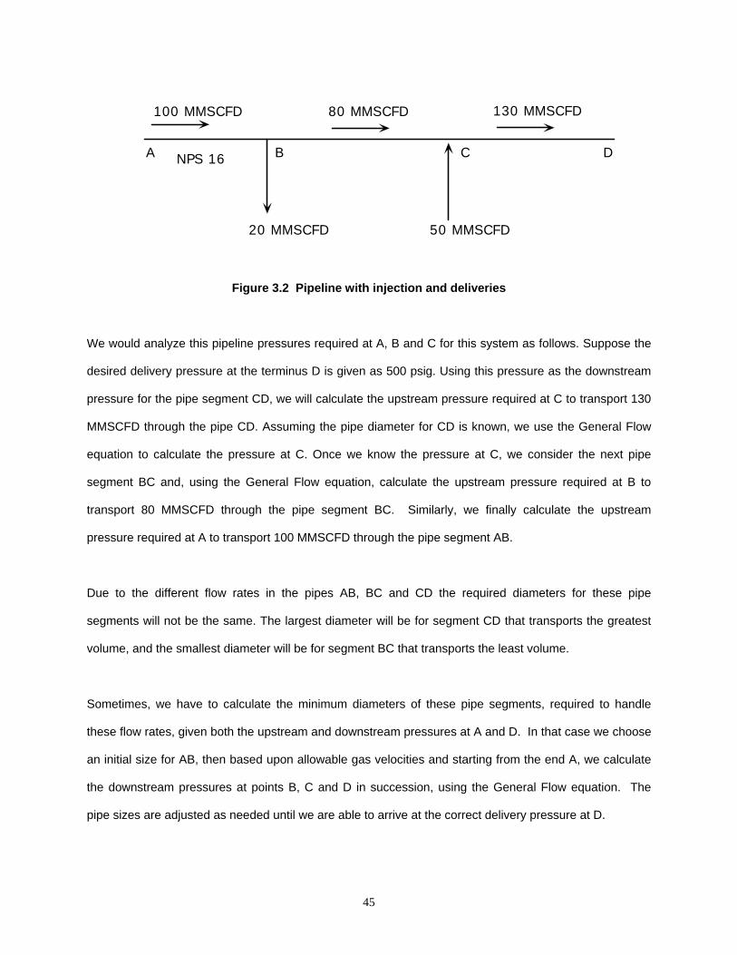
Consider a pipeline shown in Fig 3.2 where the gas enters the pipeline at A at 100 MMSCFD, and at

some point B, 20 MMSCFD is delivered to a customer. The remaining 80 MMSCFD continues to a point C

where an additional volume of 50 MMSCFD is injected into the pipeline. From that point the total volume

of 130 MMSCFD continues to the end of the pipeline at D, where it is delivered to an industrial plant at a

pressure of 800 psig.

45

Figure 3.2 Pipeline with injection and deliveries

We would analyze this pipeline pressures required at A, B and C for this system as follows. Suppose the

desired delivery pressure at the terminus D is given as 500 psig. Using this pressure as the downstream

pressure for the pipe segment CD, we will calculate the upstream pressure required at C to transport 130

MMSCFD through the pipe CD. Assuming the pipe diameter for CD is known, we use the General Flow

equation to calculate the pressure at C. Once we know the pressure at C, we consider the next pipe

segment BC and, using the General Flow equation, calculate the upstream pressure required at B to

transport 80 MMSCFD through the pipe segment BC. Similarly, we finally calculate the upstream

pressure required at A to transport 100 MMSCFD through the pipe segment AB.

Due to the different flow rates in the pipes AB, BC and CD the required diameters for these pipe

segments will not be the same. The largest diameter will be for segment CD that transports the greatest

volume, and the smallest diameter will be for segment BC that transports the least volume.

Sometimes, we have to calculate the minimum diameters of these pipe segments, required to handle

these flow rates, given both the upstream and downstream pressures at A and D. In that case we choose

an initial size for AB, then based upon allowable gas velocities and starting from the end A, we calculate

the downstream pressures at points B, C and D in succession, using the General Flow equation. The

pipe sizes are adjusted as needed until we are able to arrive at the correct delivery pressure at D.

BA D

100 MMSCFD

20 MMSCFD

NPS 16

80 MMSCFD 130 MMSCFD

C

50 MMSCFD

46

When pipes of different diameters are connected together end to end, they are referred to as series

pipes. If the flow rate is the same throughout the system, we can simplify calculations by converting the

entire system into one long piece of pipe with the same uniform diameter, using the equivalent length

concept. We calculate the equivalent length of each pipe segment (for the same pressure drop) based on

a fixed base diameter. For example a pipe of diameter D1 and length L1 will be converted to an equivalent

length Le1 of some base diameter D. This will be based on the same pressure drop in both pipes.

Similarly the remaining pipe segments, such as the pipe diameter D2 and length L2 will be converted to a

corresponding equivalent length Le2 of diameter D. Continuing the process we have the entire piping

system reduced to the following total equivalent length of the same diameter D as follows:

Total equivalent length = Le1 + Le2 + Le3 +…..

The base diameter D may be one of the segment diameters. For example, we may pick the base

diameter to be D1. Therefore the equivalent length becomes:

Total equivalent length = L1 + Le2 + Le3 +…..

From the General Flow equation, we see that the pressure drop versus the pipe diameter relationship is

such that ( )22

21 PP − is inversely proportional to the fifth power of the diameter and directly proportional

to the pipe length. Therefore, we can state the following:

5DCLPsq =∆ (3.1)

where:

∆Psq = (P1 2 – P2

2) for pipe segment.

P1, P2 = Upstream and downstream pressures of pipe segment, psia.

C = A constant

L = pipe segment length

D = pipe segment inside diameter

Therefore for the equivalent length calculations, we can state that for the second segment:

47

5

2

122 ⎟⎟

⎠

⎞⎜⎜⎝

⎛=

DD

LLe (3.2)

And for the third pipe segment the equivalent length is:

5

3

133 ⎟⎟

⎠

⎞⎜⎜⎝

⎛=

DD

LLe (3.3)

Therefore the total equivalent length Le for all pipe segments in terms of diameter D1 can be stated as:

5

3

13

5

2

121 ⎟⎟

⎠

⎞⎜⎜⎝

⎛+⎟⎟

⎠

⎞⎜⎜⎝

⎛+=

DD

LDD

LLLe + …. (3.4)

We are thus able to reduce the series pipe system to one of fixed diameter and equivalent length. The

analysis then would be easy since all pipe sizes will be the same. However, if the flow rates are different

in each section, there is really no benefit in calculating the equivalent length, since we have to consider

each segment separately and apply the General Flow equation for each flow rate. Therefore the

equivalent length approach is useful only if the flow rate is the same throughout the series piping system.

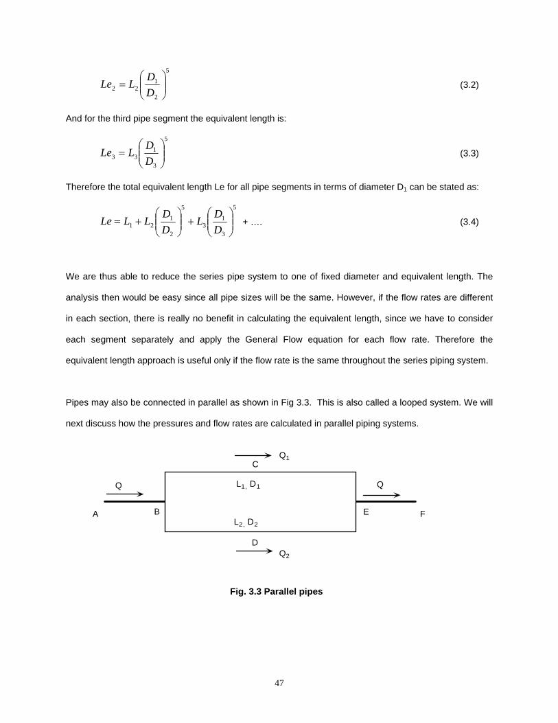
Pipes may also be connected in parallel as shown in Fig 3.3. This is also called a looped system. We will

next discuss how the pressures and flow rates are calculated in parallel piping systems.

Fig. 3.3 Parallel pipes

FA B

C

D

E

Q1

Q2

Q QL1, D1

L2, D2

48

In Fig 3.3 we have a pipe segment AB connected to two other pipes (BCE and BDE) in parallel, forming a

loop. The two pipes rejoin at E to form a single pipe segment EF. We can replace the two pipe segments

BCE and BDE by one pipe segment of some length Le and diameter De. This will be based on the same

pressure drop through the equivalent piece of pipe as the individual pipes BCE and BDE. The flow rate Q

through AB is split into two flows Q1 and Q2 as shown in the figure, such that Q1 + Q2 = Q.

Since B and E are the common junctions for each of the parallel pipes, there is a common pressure drop

∆P for each pipe BCE or BDE. Therefore the flow rate Q1 through pipe BCE results in pressure drop ∆P

just as the flow rate Q2 through pipe BDE results in the same pressure drop ∆P. The equivalent pipe of

length Le and diameter De must also have the same drop ∆P at the total flow Q, in order to completely

replace the two pipe loops. Using this principle, and noting the pressure versus diameter relationship

from the General Flow equation, we can calculate the equivalent diameter De based on setting Le equal

to the length of one of the loops BCE or BDE.

Another approach to solving the flows and pressures in a looped system is to calculate the flows Q1 and

Q2 based on the fact that the flows should total Q and the fact that there is a common pressure drop ∆P

across the two parallel segments.

Using the General Flow equation, for common ∆P, we can state that:

52

222

51

211

DQL

DQL

= (3.5)

where L1 and L2 are the two pipe segment lengths for BCE and BDE and D1 and D2 are the corresponding

inside diameters.

Simplifying the preceding equation, we get:

5.2

2

1

5.0

1

2

2

1⎟⎟⎠

⎞⎜⎜⎝

⎛⎟⎟⎠

⎞⎜⎜⎝

⎛=

DD

LL

QQ

(3.6)

Also

Q = Q1 + Q2 (3.7)

49

Using the two preceding equations, we can solve for the two flows Q1 and Q2. Once we know these flow

rates, the pressure drop in each of the pipe loops BCE or BDE can be calculated.

Looping a gas pipeline effectively increases pipe diameter, and hence results in increased throughput

capability. If a 50 mile section of NPS 16 pipeline is looped using an identical pipe size, the effective or

the equivalent diameter De and length Le are related as follows from the preceding Eq. (3.5):

52

222

51

211

5

2

DQL

DQL

DQL

e

e ==

By setting the length L1, L2 and Le to equal 50 miles, the equivalent diameter De may be calculated, after

some simplification and using Eq.(3.6), and (3.7) as follows:

25.2

2

152

5 1⎥⎥⎦

⎤

⎢⎢⎣

⎡⎟⎟⎠

⎞⎜⎜⎝

⎛+=

DDDDe

Since the loop diameters are the same, D1 = D2 = 15.5 in, assume a wall thickness of 0.25 in.

Solving for the equivalent diameter, we get:

25.255

5.155.1515.15

⎥⎥⎦

⎤

⎢⎢⎣

⎡⎟⎠⎞

⎜⎝⎛+=eD

Or De = 20.45 in.

Compared to the unlooped pipe, the looped pipeline will have an increased capacity of approximately:

QL/Q = (20.45/15.5)2.5 = 2.0

We have thus demonstrated that by looping the pipeline, the throughput can be increased to twice the

original value. Suppose instead of looping the NPS 16 pipe with an identical diameter pipe, we looped it

with NPS 20 pipe with a wall thickness of 0.375 inch, the equivalent diameter becomes:

De = 23.13 inch

And the increased capacity ratio becomes:

QL/Q = (23.13/15.5)2.5 = 2.72

50

Thus by looping the NPS 16 pipe with a NPS 20 pipe, the capacity can be increased to 2.72 times the

original throughput. This method of increasing pipeline capacity by looping involves initial capital

investment but no increased HP, such as that when we install a compressor. Thus we can compare the

cost of looping a pipeline with installing additional compressor stations.

51

4. Compressor Stations and HP

Compressor stations provide the pressure required to transport the gas in a pipeline from one location to

another. Suppose that a 20 mile long pipeline requires 1000 psig pressure at the pipe inlet A to deliver

the gas at 100 MMSCFD flow rate to the terminus B at 900 psig. If the gas at A is at 800 psig pressure, it

needs to be compressed to 1000 psig using a compressor located at A. The compressor is said to

provide a compression ratio of 7.148007.141000

++

= 1.25. Note that pressures must be converted to the

absolute pressures and hence the reason for adding 14.7, the base pressure, to the given pressures. We

say that the compressor suction pressure is 814.7 psia and the discharge pressure is 1014.7 psia.

Suppose the gas inlet temperature on the compressor suction side is 80 OF. Because of the compression

process, the gas temperature at the compressor discharge will increase, just like the discharge pressure.

If the compression process is adiabatic or isentropic, pressure versus volume will obey the adiabatic

compression equation as follows:

PVγ = constant (4.1)

where γ is the ratio of the specific heats (Cp/Cv) of the gas. This ratio is approximately 1.29 for natural

gas. Using the above equation in conjunction with the ideal gas equation, we can write a relationship

between the pressure P and the temperature T for the compression process as follows:

Constant1

=−

TP γγ

(4.2)

If the suction conditions are represented by the subscript 1 and the discharge conditions by the subscript

2, the discharge temperature of the compressed gas can be calculated as follows:

γ

γ 1

1

2

1

2

−

⎟⎟⎠

⎞⎜⎜⎝

⎛=⎟⎟

⎠

⎞⎜⎜⎝

⎛PP

TT

(4.3)

where all temperatures are in OR and the pressures are in psia.

Taking into account the compressibility of the gas, the temperature ratio above becomes:

γ

γ 1

1

2

2

1

1

2

−

⎟⎟⎠

⎞⎜⎜⎝

⎛⎟⎟⎠

⎞⎜⎜⎝

⎛=⎟⎟

⎠

⎞⎜⎜⎝

⎛PP

ZZ

TT

(4.4)

52

where Z1 and Z2 are gas compressibility factor at suction and discharge conditions, respectively.

When the compression process is polytropic, we use the polytropic coefficient n instead of g and the

temperature ratio then becomes:

n

n

PP

ZZ

TT

1

1

2

2

1

1

2

−

⎟⎟⎠

⎞⎜⎜⎝

⎛⎟⎟⎠

⎞⎜⎜⎝

⎛=⎟⎟

⎠

⎞⎜⎜⎝

⎛ (4.5)

Horsepower required

The compressors compress the natural gas and raise its pressure (and its temperature) to the level

required to ensure that the gas will be transported from point A to point B, such that the required outlet

pressure can be maintained. The higher the outlet pressure at B, the higher will be the pressure required

at A. This will cause the compressors to work harder. The energy input to the gas by the compressors

will depend upon the compression ratio and gas flow rate, among other factors. From the energy input to

the gas, we can calculate the horsepower (HP) needed.

The following equation may be used to calculate the compressor HP.

⎥⎥⎥

⎦

⎤

⎢⎢⎢

⎣

⎡−⎟⎟

⎠

⎞⎜⎜⎝

⎛⎟⎟⎠

⎞⎜⎜⎝

⎛⎟⎠⎞

⎜⎝⎛ +

⎟⎟⎠

⎞⎜⎜⎝

⎛−

=

−

1121

0857.0

1

1

2211

γγ

ηγγ

PPZZQTHP

a

(4.6)

where:

HP = compression horsepower

γ = Cp/Cv the ratio of specific heats of gas

Q = gas flow rate, MMSCFD

T1 = suction temperature of gas, OR

P1 =suction pressure of gas, psia

P2 = discharge pressure of gas, psia

Z1 = compressibility of gas at suction conditions, dimensionless

Z2 = compressibility of gas at discharge conditions, dimensionless

ηa = compressor adiabatic (isentropic) efficiency, decimal value

53

In SI units, the compressor Power required is as follows:

⎥⎥⎥

⎦

⎤

⎢⎢⎢

⎣

⎡−⎟⎟

⎠

⎞⎜⎜⎝

⎛⎟⎟⎠

⎞⎜⎜⎝

⎛⎟⎠⎞

⎜⎝⎛ +

⎟⎟⎠

⎞⎜⎜⎝

⎛−

=

−

1121

0639.4

1

1

2211

γγ

ηγγ

PPZZQTPower

a

(4.7)

where:

Power = compression Power, kW

Q = gas flow rate, Mm3/day

T1 = suction temperature of gas, K

P1 = suction pressure of gas, kPa

P2 = discharge pressure of gas, kPa

Other symbols are the same as defined previously.

The adiabatic efficiency, also called the isentropic efficiency, is approximately 0.75 to 0.85. Taking into

account a mechanical efficiency ηm of the compressor driver, the Brake Horsepower (BHP) required may

be calculated as follows:

m

HPBHPη

= (4.8)

The mechanical efficiency ηm of the driver generally varies from 0.95 to 0.98. By multiplying the two

efficiencies, we get the overall efficiency ηo as follows:

ηo = ηa x ηm (4.9)

The adiabatic efficiency can be calculated, knowing the actual discharge temperature of the gas, suction

and discharge pressures and the compressibility factors, using the following equation:

⎥⎥⎥

⎦

⎤

⎢⎢⎢

⎣

⎡−⎟⎟

⎠

⎞⎜⎜⎝

⎛⎟⎟⎠

⎞⎜⎜⎝

⎛⎟⎟⎠

⎞⎜⎜⎝

⎛−

=

−

1

1

1

2

2

1

12

1γ

γ

ηPP

ZZ

TTT

a (4.10)

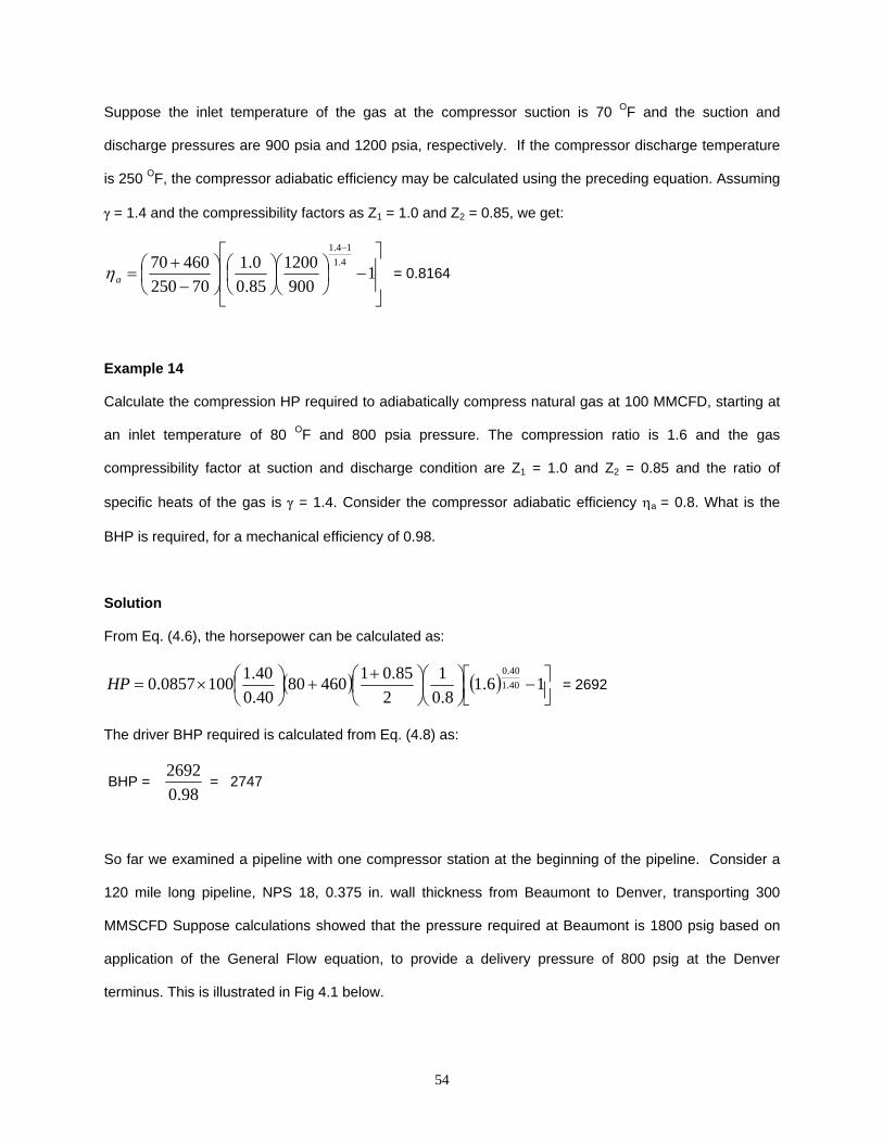
54

Suppose the inlet temperature of the gas at the compressor suction is 70 OF and the suction and

discharge pressures are 900 psia and 1200 psia, respectively. If the compressor discharge temperature

is 250 OF, the compressor adiabatic efficiency may be calculated using the preceding equation. Assuming

γ = 1.4 and the compressibility factors as Z1 = 1.0 and Z2 = 0.85, we get:

⎥⎥

⎦

⎤

⎢⎢

⎣

⎡−⎟

⎠⎞

⎜⎝⎛

⎟⎠⎞

⎜⎝⎛

⎟⎠⎞

⎜⎝⎛

−+

=

−

1900

120085.00.1

7025046070 4.1

14.1

aη = 0.8164

Example 14

Calculate the compression HP required to adiabatically compress natural gas at 100 MMCFD, starting at

an inlet temperature of 80 OF and 800 psia pressure. The compression ratio is 1.6 and the gas

compressibility factor at suction and discharge condition are Z1 = 1.0 and Z2 = 0.85 and the ratio of

specific heats of the gas is γ = 1.4. Consider the compressor adiabatic efficiency ηa = 0.8. What is the

BHP is required, for a mechanical efficiency of 0.98.

Solution

From Eq. (4.6), the horsepower can be calculated as:

( ) ( ) ⎥⎦⎤

⎢⎣⎡ −⎟

⎠⎞

⎜⎝⎛

⎟⎠⎞

⎜⎝⎛ +

+⎟⎠⎞

⎜⎝⎛×= 16.1

8.01

285.0146080

40.040.11000857.0 40.1

40.0HP = 2692

The driver BHP required is calculated from Eq. (4.8) as:

BHP = 98.0

2692 = 2747

So far we examined a pipeline with one compressor station at the beginning of the pipeline. Consider a

120 mile long pipeline, NPS 18, 0.375 in. wall thickness from Beaumont to Denver, transporting 300

MMSCFD Suppose calculations showed that the pressure required at Beaumont is 1800 psig based on

application of the General Flow equation, to provide a delivery pressure of 800 psig at the Denver

terminus. This is illustrated in Fig 4.1 below.

55

Figure 4.1 Compressor stations required

If the maximum allowable operating pressure (MAOP) of the pipeline is limited to 1400 psig, we cannot

just install one compressor station at the beginning to provide the necessary pressure, since the 1800

psig is beyond the pipe MAOP. Therefore, by installing an additional intermediate compressor station at

Grover, as shown in the figure, we can keep each compressor station discharge pressure at the MAOP

limit. The location of the Grover compressor station will depend upon the MAOP, the allowable

compression ratio and the suction pressure. One approach is to calculate the distance x between Grover

and Denver, such that starting at 1400 psig at Grover, the gas outlet pressure at Denver is exactly 800

psig. We would apply the General Flow equation to the x mile length of pipe with upstream pressure set

at P1 = (1400 + 14.7) psia and downstream pressure P2 = (800 +14.7) psia.

Having calculated the value of x and hence the location of Grover, we must calculate the suction pressure

at Grover, by considering the pipe segment between Beaumont and Grover. If the suction pressure at

Grover is too low, the compression ratio for the Grover compressor will be too high. Generally the

compression ratio is limited to 1.2 to 1.8 for centrifugal compressors. If the suction pressure at Grover is

Beaumont Denver

NPS 18 pipeline 120 miles long

800 psig

Flow

1800 psig

Grover

1400 psig1400 psig

1000 psig

Distance

56

too low, we will have to consider installing two (2) intermediate compressors instead of one at Grover.

These two compressor stations will be located such that the suction pressures do not fall too low and the

compression ratio is within limits.

57

5. Strength of Pipe

In earlier sections of this course, we calculated the pressures and flow rates in a natural gas pipeline.

Using the flow equations, we calculated the minimum pressure required to transport gas at a certain flow

rate and temperature from one point to another. The pipe used for transportation of gas should be able to

withstand the necessary internal pressure. The internal pressure in a pipe is limited to what the pipe

material and wall thickness can withstand at a certain temperature. As the pipe pressure is increased,

the stress in the pipe material increases. Ultimately, at some internal pressure the pipe will rupture.

Therefore for each pipe size and wall thickness, depending upon the pipe material, there is a safe internal

pressure beyond which it is not advisable to operate the pipeline. This is known as the maximum

allowable operating pressure (MAOP), sometimes shortened to maximum operating pressure (MOP).

There are two stresses developed in a pipe wall due to internal pressure. The larger of the two is called

the hoop stress and acts in the circumferential direction. The second is the axial or longitudinal stress that

acts along the axial direction. The axial stress is one-half the magnitude of the hoop stress. This is

illustrated in the Fig. 5.1.

Hoop Stress - Sh

Axial Stre

ss - Sa

Axial Stress - Sa

Pressure - P

Sh

Diameter - D

Fig 5.1 Pipe stresses due to internal pressure

The allowable internal pressure can be easily calculated using the Barlow’s equation as follows:

58

t

PDSh 2= (5.1)

where:

Sh = allowable hoop stress in pipe, psig

P = allowable internal pressure, psig

D = pipe outside diameter, in.

t = pipe wall thickness, in.

Even though the Barlow’s equation is for calculating the hoop stress in the pipe for a given internal

pressure, we can easily re-arrange the equation to solve for the pressure P.

DtSP h2

= (5.2)

Thus for an NPS 20 pipe, 0.500 in. wall thickness, if the allowable hoop stress is limited to 30,000 psig,

the allowable internal pressure is:

P = 150020

000,305.02=

×× psig

The longitudinal stress, Sa, can be calculated from a similar equation as follows:

t

PDSa 4= (5.3)

It must be noted that unlike the General Flow equation or other flow equations, the diameter used here is

the outside diameter, not the inside diameter. In practice, to calculate the internal design pressure for a

gas pipeline, we modify the Barlow’s equation slightly by introducing some factors that depend upon the

pipeline manufacturing method, operating temperature and the class location of the pipeline. The

modified equation is as follows:

D

tSEFTP 2= (5.4)

where:

P = internal design pressure, psig

D = outside diameter of pipe, in.

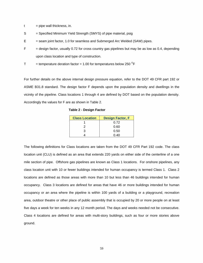
59

t = pipe wall thickness, in.

S = Specified Minimum Yield Strength (SMYS) of pipe material, psig

E = seam joint factor, 1.0 for seamless and Submerged Arc Welded (SAW) pipes.

F = design factor, usually 0.72 for cross country gas pipelines but may be as low as 0.4, depending

upon class location and type of construction.

T = temperature deration factor = 1.00 for temperatures below 250 OF

For further details on the above internal design pressure equation, refer to the DOT 49 CFR part 192 or

ASME B31.8 standard. The design factor F depends upon the population density and dwellings in the

vicinity of the pipeline. Class locations 1 through 4 are defined by DOT based on the population density.

Accordingly the values for F are as shown in Table 2.

Table 2 - Design Factor

Class Location Design Factor, F 1 0.72 2 0.60 3 0.50 4 0.40

The following definitions for Class locations are taken from the DOT 49 CFR Part 192 code. The class

location unit (CLU) is defined as an area that extends 220 yards on either side of the centerline of a one

mile section of pipe. Offshore gas pipelines are known as Class 1 locations. For onshore pipelines, any

class location unit with 10 or fewer buildings intended for human occupancy is termed Class 1. Class 2

locations are defined as those areas with more than 10 but less than 46 buildings intended for human

occupancy. Class 3 locations are defined for areas that have 46 or more buildings intended for human

occupancy or an area where the pipeline is within 100 yards of a building or a playground, recreation

area, outdoor theatre or other place of public assembly that is occupied by 20 or more people on at least

five days a week for ten weeks in any 12 month period. The days and weeks needed not be consecutive.

Class 4 locations are defined for areas with multi-story buildings, such as four or more stories above

ground.

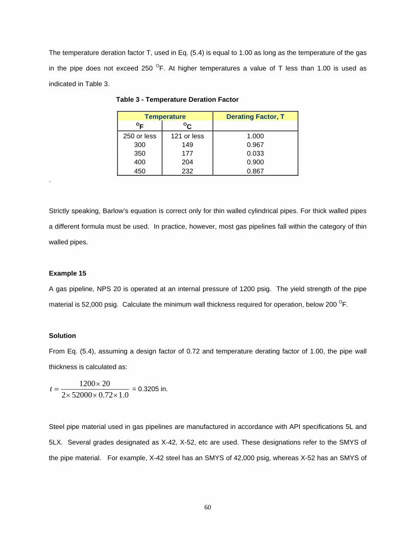
60

The temperature deration factor T, used in Eq. (5.4) is equal to 1.00 as long as the temperature of the gas

in the pipe does not exceed 250 OF. At higher temperatures a value of T less than 1.00 is used as

indicated in Table 3.

Table 3 - Temperature Deration Factor

Temperature Derating Factor, T OF OC

250 or less 121 or less 1.000 300 149 0.967 350 177 0.033 400 204 0.900 450 232 0.867

.

Strictly speaking, Barlow’s equation is correct only for thin walled cylindrical pipes. For thick walled pipes

a different formula must be used. In practice, however, most gas pipelines fall within the category of thin

walled pipes.

Example 15

A gas pipeline, NPS 20 is operated at an internal pressure of 1200 psig. The yield strength of the pipe

material is 52,000 psig. Calculate the minimum wall thickness required for operation, below 200 OF.

Solution

From Eq. (5.4), assuming a design factor of 0.72 and temperature derating factor of 1.00, the pipe wall

thickness is calculated as:

0.172.0520002201200

××××

=t = 0.3205 in.

Steel pipe material used in gas pipelines are manufactured in accordance with API specifications 5L and

5LX. Several grades designated as X-42, X-52, etc are used. These designations refer to the SMYS of

the pipe material. For example, X-42 steel has an SMYS of 42,000 psig, whereas X-52 has an SMYS of

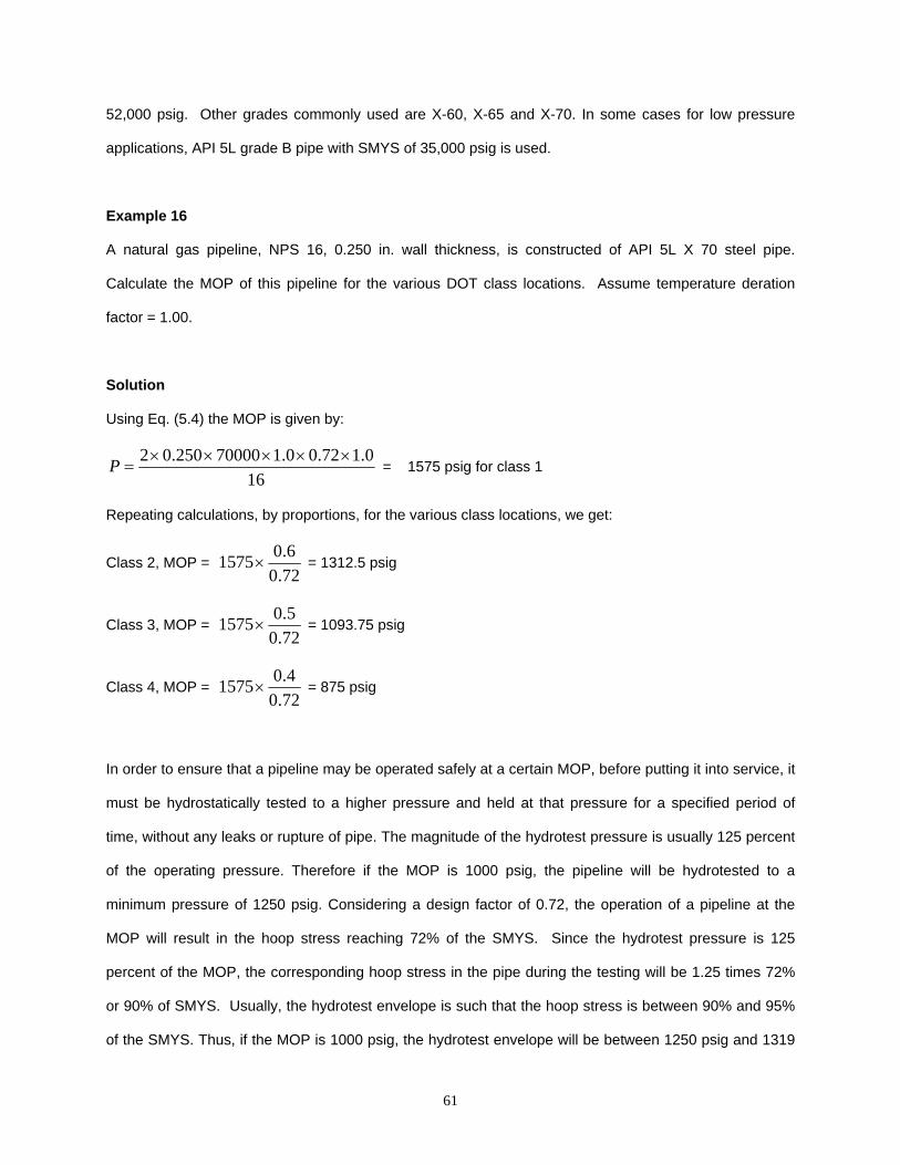
61

52,000 psig. Other grades commonly used are X-60, X-65 and X-70. In some cases for low pressure

applications, API 5L grade B pipe with SMYS of 35,000 psig is used.

Example 16

A natural gas pipeline, NPS 16, 0.250 in. wall thickness, is constructed of API 5L X 70 steel pipe.

Calculate the MOP of this pipeline for the various DOT class locations. Assume temperature deration

factor = 1.00.

Solution

Using Eq. (5.4) the MOP is given by:

160.172.00.170000250.02 ×××××

=P = 1575 psig for class 1

Repeating calculations, by proportions, for the various class locations, we get:

Class 2, MOP = 72.06.01575× = 1312.5 psig

Class 3, MOP = 72.05.01575× = 1093.75 psig

Class 4, MOP = 72.04.01575× = 875 psig

In order to ensure that a pipeline may be operated safely at a certain MOP, before putting it into service, it

must be hydrostatically tested to a higher pressure and held at that pressure for a specified period of

time, without any leaks or rupture of pipe. The magnitude of the hydrotest pressure is usually 125 percent

of the operating pressure. Therefore if the MOP is 1000 psig, the pipeline will be hydrotested to a

minimum pressure of 1250 psig. Considering a design factor of 0.72, the operation of a pipeline at the

MOP will result in the hoop stress reaching 72% of the SMYS. Since the hydrotest pressure is 125

percent of the MOP, the corresponding hoop stress in the pipe during the testing will be 1.25 times 72%

or 90% of SMYS. Usually, the hydrotest envelope is such that the hoop stress is between 90% and 95%

of the SMYS. Thus, if the MOP is 1000 psig, the hydrotest envelope will be between 1250 psig and 1319

62

psig. For buried pipelines, the hydrotest pressure is held constant for a period of 8 hours and it is

thoroughly checked for leaks. For above ground pipelines, the hydrotest period is 4 hours.

Frequently, in gas pipeline hydraulics, we are interested in knowing the quantity of pipe required for a

project. There is a simple formula for calculating the weight of pipe per unit length of pipe. For a given

pipe of outside diameter D and wall thickness t, the weight per foot of pipe is given by:

w = 10.68 t (D-t) (5.5)

where D and t are in inches and w is in lb/ft.

For example, a 20 mile pipeline, and NPS 20 with 0.500 in wall thickness, has a total pipe weight of:

W = 20 x 5280 x 10.68 x 0.500 x (20-0.5) = 10,996,128 lb or 5,498 tons

Summary

In this course we addressed the hydraulics of compressible fluids such as natural gases. First we

introduced the relevant properties of gas that affect pipeline hydraulics. Next, the methods of calculating

pressures and flow rates in a natural gas pipeline was analyzed, with reference to several popular

equation of gas flow. We compared the various flow equations and found some were more conservative

than others. Using the pressure calculated, the compressor HP was estimated. The need for installing

additional intermediate compressor stations, based on allowable pipe pressures, was explained.

Methods of increasing pipeline throughput were discussed. The strength requirement of pipes to

withstand the internal pressure was reviewed using the Barlow’s equation.

63

References

1. Pipeline Engineering, 2003, CRC Press, Florida, Henry Liu

2. Flow of Fluids through Valves, Fittings and Pipe, 1976, Crane Company, New York

3. Fundamentals of Pipe Flow, 1980, John Wiley and Sons, New York, Robert P. Benedict

4. The Properties of Petroleum Fluids, 1973, Petroleum Publishing Company, Tulsa, William D. McCain,

Jr.

5. Engineering Data Book, Tenth Edition, 1994, Gas Processors Suppliers Association, Tulsa, Oklahoma.