Course introduction G. Ferrari Trecate -...

Nonlinear systemsCourse introduction

G. Ferrari Trecate

Dipartimento di Ingegneria Industriale e dell’InformazioneUniversita degli Studi di Pavia

Advanced automation and control

Ferrari Trecate (DIS) Nonlinear systems Advanced autom. and control 1 / 38

Course schedule

Advanced automation and control

Industrial automation + Nonlinear systems

Lectures

Monday 14-16 room EF3, Thursday 16-18, room E1 (Industrialautomation)

Wednesday 14-16, room E1 (Nonlinear systems)

Office hours

By appointment ([email protected]). Office:Dipartimento di Ingegneria Industriale e dell’Informazione, floor F


[email protected]

Course website

http:

//sisdin.unipv.it/labsisdin/teaching/courses/ails/files/ails.php

a copy of the slides can be downloaded after authentication withlogin/password


http://sisdin.unipv.it/labsisdin/teaching/courses/ails/files/ails.php

http://sisdin.unipv.it/labsisdin/teaching/courses/ails/files/ails.php

Textbooks

For a review of basic systems theory and automatic control

G. F. Franklin, J. D. Powell, A. Emami-Naeini. Feedback Control ofDynamic Systems 6th ed., 2009 Prentice Hall

P. Bolzern, R. Scattolini, N. Schiavoni. Fondamenti di Controlli Automatici,2nd ed., 2004, McGraw-Hill, Italia

For the topics in nonlinear systems covered in the course

J.-J. E. Slotine e W. Li. Applied nonlinear control. Prentice-Hall (1991)

H.K. Khalil. Nonlinear systems - third edition. Prentice-Hall (2002)

S. Sastry. Nonlinear systems - Analysis, Stability and Control.Springer-Verlag (1999) (and C. Tomlin - slides of the course “AdvancedNonlinear Control”, Stanford University)

All above books cover several topics that will be not discussed in the course.Khalil an Sastry’s books are the most advanced (and difficult) ones

The exam will focus only on topics covered in the course


Exams

Closed-books closed-notes written exam split in two parts

First part: industrial automation

Second part: nonlinear systems

Total duration: ∼ 3h. No graphic or programmable calculators are allowed

Registration to exams

Through the university website

Usually, registrations end 7 days before the exam date


Nonlinear (NL) systems

Analysis vs. simulation

Steadily increasing computing power allows one to simulate complexNL systems

Simulation and intuition allow one to understand several aspects ofNL systems

However,

Impossible to use only simulation to prove interesting properties (e.g.stability)

Analysis procedures allow properties of NL systems to be rigorouslyassessed

I Sometimes, results are surprising and highlight behaviors one had nottought to simulate !


Nonlinear (NL) systems

NL systems vs. linear systems

Several results on the analysis and control of linear systemsHOWEVER

Most real systems are NL

Linear systems do not capture behaviors such asI isolated multiple equilibriaI limit cyclesI subharmonicsI complex dynamics, e.g. chaos

Next ...

Review of systems theory !

Examples of nonlinear behaviors


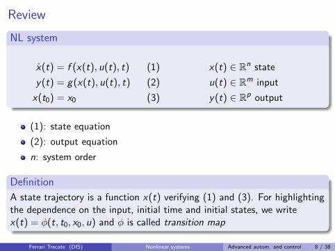
Review

NL system

x(t) = f (x(t), u(t), t) (1)

y(t) = g(x(t), u(t), t) (2)

x(t0) = x0 (3)

x(t) ∈ Rn state

u(t) ∈ Rm input

y(t) ∈ Rp output

(1): state equation

(2): output equation

n: system order

Definition

A state trajectory is a function x(t) verifying (1) and (3). For highlightingthe dependence on the input, initial time and initial states, we writex(t) = φ(t, t0, x0, u) and φ is called transition map


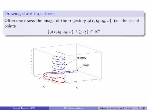
Drawing state trajectories

Often one draws the image of the trajectory φ(t, t0, x0, u), i.e. the set ofpoints

{φ(t, t0, x0, u), t ≥ t0} ⊂ Rn

02

46

810

2

4

6

8

10

0

5

10

15

20

25

30

35

40

x1

x2

t

Trajectory

Image


Review

NL system

x(t) = f (x(t), u(t), t)

y(t) = g(x(t), u(t), t)

x(t0) = x0

x(t) ∈ Rn

u(t) ∈ Rm

y(t) ∈ Rp

An NL system is:

Invariant if f and g do not depend upon timeI Without loss of generality, one can set t0 = 0 andφ(t, t0, x0, u) = φ(t, x0, u)

Autonomous if the system does not depend upon the input u(t)I φ(t, t0, x0, u) = φ(t, t0, x0)

Invariant and autonomous: x(t) = f (x(t)), y(t) = g(x(t))I φ(t, t0, x0, u) = φ(t, x0)

Static if n = 0I described only through the output equation y(t) = g(u(t), t)


Review of linear systems

A system is linear if f and g are linear functions of x and u

x(t) = A(t)x(t) + B(t)u(t)

y(t) = C (t)x(t) + D(t)u(t)

A(t), B(t), C (t), D(t) matrices

Linear Time-Invariant (LTI) system

x(t) = Ax(t) + Bu(t)

y(t) = Cx(t) + Du(t)

A, B, C , D matrices


Multiple isolated equilibria


NL vs. linear systems: Duffing oscillator

Model

ml2x1 = mgl sin(x1)− αx1 − kx1 + τ

−αx1: restoring torque (α > 0)

−kx1: damping torque (k > 0)

τ : electromagnetic torque (input)

NL system

Defining x2 = x1, u =τ

ml2,

x1 = x2

x2 =g

lsin(x1)−

α

ml2x1 −

k

ml2x2 + u


Review

Equilibrium

Given u(t) = u, ∀t ≥ 0, the state x ∈ Rn is an equilibrium state for thenonlinear time-invariant system x = f (x , u) if it verifies f (x , u) = 0a. Thepair (x , u) is called an equilibrium.

ax = x2 + 1, x(t) ∈ R has no equilibrium state

Duffing oscillator: equilibra for u = 0

Physical intuition: 3 equilibra


Duffing oscillator: equilibria of approximate models

NL system

x1 = x2

x2 =g

lsin(x1)−

α

ml2x1 −

k

ml2x2 + u

Linear approximation: sin(x1) ' x1

LTI system (u = 0)

x1 = x2

x2 =

(g

l−

α

ml2

)x1 −

k

ml2x2

Equilibrium states:

x2 = 0(g

l−

α

ml2

)6= 0⇒ x1 = 0

Either one or infinite equilibrium states


Duffing oscillator: equilibria of approximate models

NL system

x1 = x2

x2 =g

lsin(x1)−

α

ml2x1 −

k

ml2x2 + u

Approximation: sin(x1) ' x1 − x31/6

Approximated NL system (u = 0)

x1 = x2

x2 =

(g

l−

α

ml2

)x1 −

g

6lx3

1 −k

ml2x2

Equilibrium states:

x2 = 0(g

l−

α

ml2

)x1 −

g

6lx3

1 = 0

One can have 3 equilibrium states


Duffing oscillator: equilibria of the approximate NL model

If we set gl −

αml2

= 1, g6l = 1, k

ml2= η, we get

Automonous Duffing model:

x1 = x2

x2 = x1 − x31 − ηx2

Equilibrium states:

p1 =

[−10

], p2 =

[00

], p3 =

[10

],


Linear approximations around anequilibrium


Review: linearization around an equilibrium

Let (x , u) be an equilibrium for the NL invariant system

x = f (x , u)

y = g(x , u)

Deviations: δx(t) = x(t)− x , δu(t) = u(t)− u, δy(t) = y(t)− y

First order Taylor expansion about the equilibrium:

f (x , u) ' f (x , u) + Dx f (x , u)∣∣∣x=xu=u

(x − x) + Duf (x , u)∣∣∣x=xu=u

(u − u)

g(x , u) ' g(x , u) + Dxg(x , u)∣∣∣x=xu=u

(x − x) + Dug(x , u)∣∣∣x=xu=u

(u − u)

Dx f (x , u) =

∂f1(x, u)

∂x1

· · ·∂f1(x, u)

∂xn...

. . ....

∂fn(x, u)

∂x1

· · ·∂fn(x, u)

∂xn

Jacobian with respect to the variables x



One gets:

˙δx = x − ˙x = f (x , u) ' f (x , u)︸︷︷︸=0

+Dx f (x , u)∣∣∣x=xu=u

δx + Duf (x , u)∣∣∣x=xu=u

δu

δy = −y + y ' −g(x , u) + g(x , u)︸︷︷︸=0

+Dxg(x , u)∣∣∣x=xu=u

δx + Dug(x , u)∣∣∣x=xu=u

δu

Linearized system

Defining

A = Dx f (x , u)∣∣∣x=xu=u

, B = Duf (x , u)∣∣∣x=xu=u

, C = Dxg(x , u)∣∣∣x=xu=u

, D = Dug(x , u)∣∣∣x=xu=u

the linearized system around the equilibrium (x , u) is

˙δx = Aδx + Bδu

δy = Cδx + DδuFerrari Trecate (DIS) Nonlinear systems Advanced autom. and control 20 / 38


We hope state trajectories of the linearized system are goodapproximations of x(t)− x ... but this does not always happen

Example: (a): x = x3, (b): x = −x3

Linearized systems around x = 0 are the same: ˙δx = 0⇒ δx(t) = x0

but NL systems have different behaviors

−1 −0.8 −0.6 −0.4 −0.2 0 0.2 0.4 0.6 0.8 1−1

−0.8

−0.6

−0.4

−0.2

0

0.2

0.4

0.6

0.8

1

Case (a)

−1 −0.8 −0.6 −0.4 −0.2 0 0.2 0.4 0.6 0.8 1−1

−0.8

−0.6

−0.4

−0.2

0

0.2

0.4

0.6

0.8

1

Case (b)


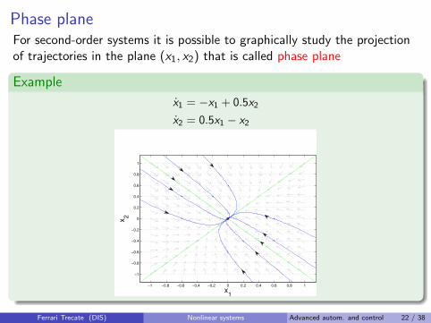
Phase planeFor second-order systems it is possible to graphically study the projectionof trajectories in the plane (x1, x2) that is called phase plane

Example

x1 = −x1 + 0.5x2

x2 = 0.5x1 − x2

−1 −0.8 −0.6 −0.4 −0.2 0 0.2 0.4 0.6 0.8 1

−1

−0.8

−0.6

−0.4

−0.2

0

0.2

0.4

0.6

0.8

1

x1

x2


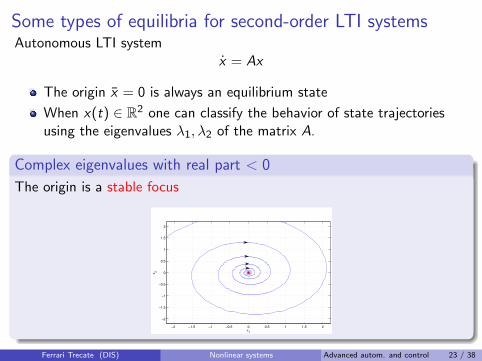
Some types of equilibria for second-order LTI systemsAutonomous LTI system

x = Ax

The origin x = 0 is always an equilibrium state

When x(t) ∈ R2 one can classify the behavior of state trajectoriesusing the eigenvalues λ1, λ2 of the matrix A.

Complex eigenvalues with real part < 0

The origin is a stable focus

−2 −1.5 −1 −0.5 0 0.5 1 1.5 2

−2

−1.5

−1

−0.5

0

0.5

1

1.5

2

x1

x2


Some types of equilibria for second-order LTI systemsAutonomous LTI system

x = Ax

The origin x = 0 is always an equilibrium state

When x(t) ∈ R2 one can classify the behavior of state trajectoriesusing the eigenvalues λ1, λ2 of the matrix A.

Real eigenvalues and λ1 < 0 < λ2

The origin is a saddle

−2 −1.5 −1 −0.5 0 0.5 1 1.5 2

−2

−1.5

−1

−0.5

0

0.5

1

1.5

2

x1

x2


Equilibria of second-order NL systems

Idea: analyze the behavior of state trajectories around an equilibrium stateusing the linearized system

Example: Duffing model for η = 1

NL system

x1 = x2

x2 = x1 − x31 − ηx2, η = 1

Linearized system

˙δx1 = δx2

˙δx2 = δx1 − 3x21 δx1 − δx2

Around p1 =[−1 0

]Tand p3 =

[1 0

]TDx f =

[0 1−2 −1

]⇒ Eigenvalues:−

1

2± j

√3

2

Can we conlude that p1 and p3 are stable foci ?


Equilibria of second-order NL systems

Around p2 =[0 0

]TDx f =

[0 11 −1

]⇒ Eigenvalues:− 1±

√5

2

Can we conlude that p2 is a saddle ?

−2.5 −2 −1.5 −1 −0.5 0 0.5 1 1.5 2 2.5

−5

−4

−3

−2

−1

0

1

2

3

4

5

x1

x2

From the state trajectories itseems the answer is yes...The analysis is local.


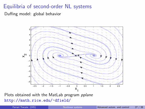
Equilibria of second-order NL systemsDuffing model: global behavior

−2.5 −2 −1.5 −1 −0.5 0 0.5 1 1.5 2 2.5

−5

−4

−3

−2

−1

0

1

2

3

4

5

x1

x2

Plots obtained with the MatLab program pplanehttp://math.rice.edu/~dfield/


http://math.rice.edu/~dfield/

Subharmonics


Subharmonics

Duffing model with input

x1 = x2

x2 = x1 − x31 − ηx2 + u

η= 0.025, u(t) = 7.5 sin(t)

0 10 20 30 40 50 60−4

−3

−2

−1

0

1

2

3

4

t

x1

Subharmonics

Harmonics that are NOT present in theinput appear in the output (even in theasymptotic regime)

Impossible for asymptotically stableLTI systems (because of thefrequency response theorem)


Chaos


Chaos

Duffing model with input

x1 = x2

x2 = x1 − x31 − ηx2 + u

η= 0.025, u(t) = 7.5 sin(t)

State trajectory x1 when x(0) = 0 and x(0) = 0 + ε

0 10 20 30 40 50 60−4

−3

−2

−1

0

1

2

3

4

t

x1

x1 perturbato

Chaos

Huge sensitivity to initialstates.

Simulations might bemeaningless


Limit cycles


Surge and rotating stall in jet engine compressorsEngine “de Havilland Goblin II”1

1Picture from WikipediaFerrari Trecate (DIS) Nonlinear systems Advanced autom. and control 33 / 38

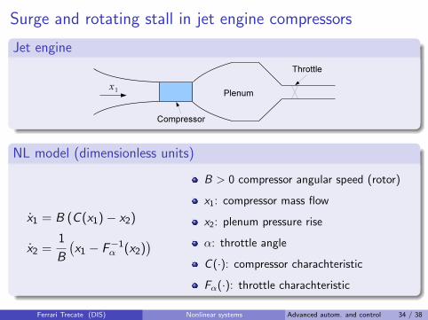
Surge and rotating stall in jet engine compressors

Jet engine

NL model (dimensionless units)

x1 = B (C (x1)− x2)

x2 =1

B

(x1 − F−1

α (x2))

B > 0 compressor angular speed (rotor)

x1: compressor mass flow

x2: plenum pressure rise

α: throttle angle

C (·): compressor charachteristic

Fα(·): throttle charachteristic


Analysis of equilibria

Computation of equilibria0 = B (C (x1)− x2)

0 =1

B

(x1 − F−1

α (x2)) ⇒

{x2 = C (x1)

x1 = F−1α (x2)

⇒ Fα(x1) = C (x1)

Equilibria for various throttle angle

0 0.5 1 1.5 2 2.5 3 3.5 40

1

2

3

4

5

6

7

8

9

10

x2

x1

Fα

3

Fα

2

Fα

1

0<α1<α

2<α

3


Unstalled operating point

0 0.5 1 1.5 2 2.5 3 3.5 40

1

2

3

4

5

6

7

8

9

10

x2

x1

This is the desired behavior: stable equilibrium


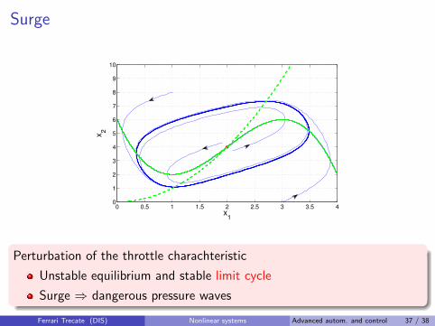
Surge

0 0.5 1 1.5 2 2.5 3 3.5 40

1

2

3

4

5

6

7

8

9

10

x2

x1

Perturbation of the throttle charachteristic

Unstable equilibrium and stable limit cycle

Surge ⇒ dangerous pressure waves


Rotating stall

0 0.5 1 1.5 2 2.5 3 3.5 40

1

2

3

4

5

6

7

8

9

10

x2

x1

Perturbation of the throttle charachteristic + decrease of the angularspeed B of the compressor

Stable equilibrium but insufficient pressure ⇒ rotating stall !


Course introduction G. Ferrari Trecate -...

Documents

Transcript of Course introduction G. Ferrari Trecate -...