COURSE INFORMATION - wbricken.com · COURSE INFORMATION Text: No text, many handouts (see below)...
92
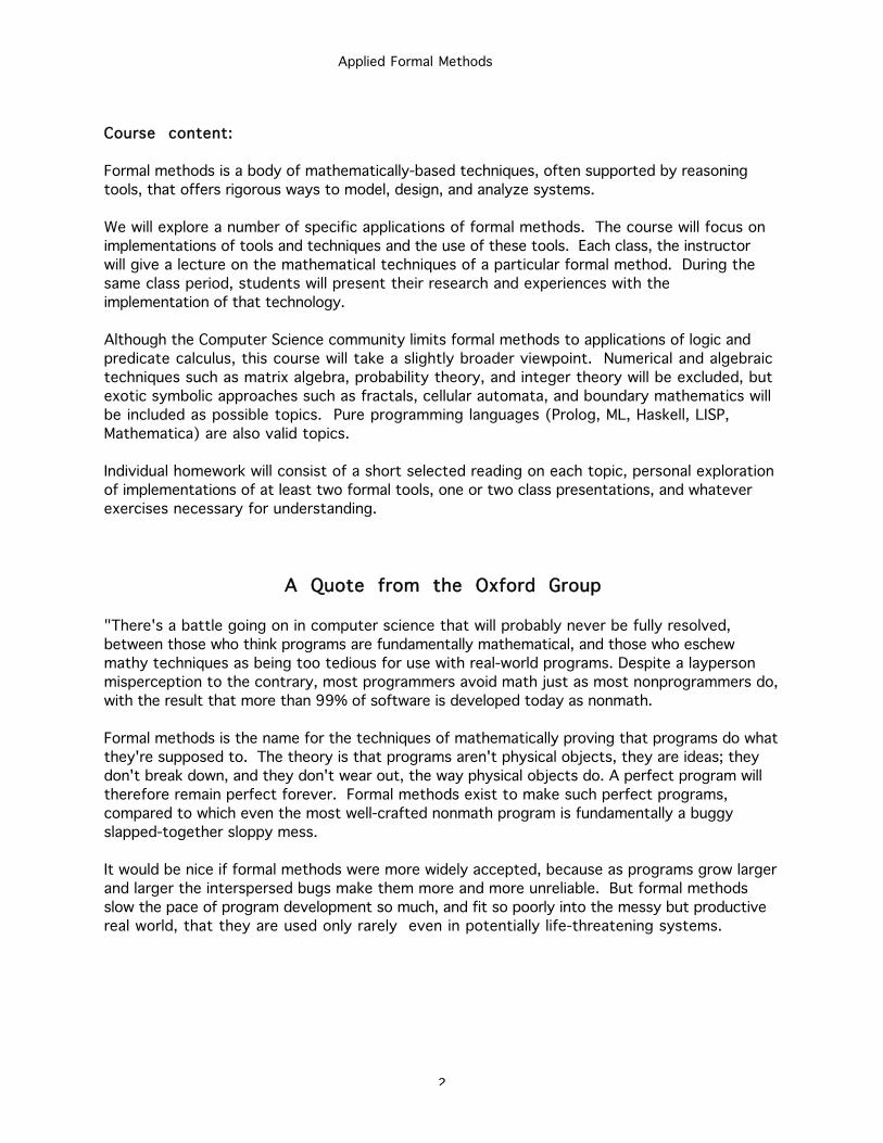
Applied Formal Methods 1 COURSE INFORMATION Text: No text, many handouts (see below) Class structure: Each student will prepare two reports on two formal methods topics. (Topic suggestions are below.) Each class period, a student and the instructor will jointly cover one selected topic. Evaluation: Available grades: non-completion: Incomplete, Withdraw, etc. completion: A A- B+ B B- C A: reserved for superior performance A- or B+: expected grade for conscientious performance B: adequate work B-: barely adequate C: equivalent to failing Grading Options: 1. Performance Quality: attendance, participation, assigned exercises 2. Grading Contract: specify a set of behaviors and an associated grade. 3. Self-determined: negotiate with instructor Discussion: If you prefer a clearly defined agenda, if you do well with concrete task assignments, or if you need a schedule of activities for motivation, then O Option 1 is a good idea. If you already understand the field, if you plan to excel in a particular area, or if you need clear performance goals for motivation, then O Option 2 is a good idea. If you are not concerned about grades, if you intend to do what you choose anyway, or if you are self-motivated, then O Option 3 is a good idea. I will notify any student who is not on a trajectory for personal success.
Transcript of COURSE INFORMATION - wbricken.com · COURSE INFORMATION Text: No text, many handouts (see below)...
Applied Formal Methods
1
COURSE INFORMATION
Text:
No text, many handouts (see below)
Class structure:
Each student will prepare two reports on two formal methods topics. (Topic suggestions
are below.) Each class period, a student and the instructor will jointly cover one
selected topic.
Eva luat ion :
Available grades:
non-completion: Incomplete, Withdraw, etc.
completion: A A- B+ B B- C
A: reserved for superior performance
A- or B+: expected grade for conscientious performance
B: adequate work
B - : barely adequate
C: equivalent to failing
Grading Options:
1. Performance Quality: attendance, participation, assigned exercises
2. Grading Contract: specify a set of behaviors and an associated grade.
3. Self-determined: negotiate with instructor
Discussion:
If you prefer a clearly defined agenda, if you do well with concrete task assignments, or
if you need a schedule of activities for motivation, then OOption 1 is a good idea.
If you already understand the field, if you plan to excel in a particular area, or if you
need clear performance goals for motivation, then OOption 2 is a good idea.
If you are not concerned about grades, if you intend to do what you choose anyway, or if
you are self-motivated, then OOption 3 is a good idea.
I will notify any student who is not on a trajectory for personal success.
Applied Formal Methods
2
Course content:
Formal methods is a body of mathematically-based techniques, often supported by reasoning
tools, that offers rigorous ways to model, design, and analyze systems.
We will explore a number of specific applications of formal methods. The course will focus on
implementations of tools and techniques and the use of these tools. Each class, the instructor
will give a lecture on the mathematical techniques of a particular formal method. During the
same class period, students will present their research and experiences with the
implementation of that technology.
Although the Computer Science community limits formal methods to applications of logic and
predicate calculus, this course will take a slightly broader viewpoint. Numerical and algebraic
techniques such as matrix algebra, probability theory, and integer theory will be excluded, but
exotic symbolic approaches such as fractals, cellular automata, and boundary mathematics will
be included as possible topics. Pure programming languages (Prolog, ML, Haskell, LISP,
Mathematica) are also valid topics.
Individual homework will consist of a short selected reading on each topic, personal exploration
of implementations of at least two formal tools, one or two class presentations, and whatever
exercises necessary for understanding.
A Quote from the Oxford Group
"There's a battle going on in computer science that will probably never be fully resolved,
between those who think programs are fundamentally mathematical, and those who eschew
mathy techniques as being too tedious for use with real-world programs. Despite a layperson
misperception to the contrary, most programmers avoid math just as most nonprogrammers do,
with the result that more than 99% of software is developed today as nonmath.
Formal methods is the name for the techniques of mathematically proving that programs do what
they're supposed to. The theory is that programs aren't physical objects, they are ideas; they
don't break down, and they don't wear out, the way physical objects do. A perfect program will
therefore remain perfect forever. Formal methods exist to make such perfect programs,
compared to which even the most well-crafted nonmath program is fundamentally a buggy
slapped-together sloppy mess.
It would be nice if formal methods were more widely accepted, because as programs grow larger
and larger the interspersed bugs make them more and more unreliable. But formal methods
slow the pace of program development so much, and fit so poorly into the messy but productive
real world, that they are used only rarely even in potentially life-threatening systems.
Applied Formal Methods
3
Some Formal Techniques
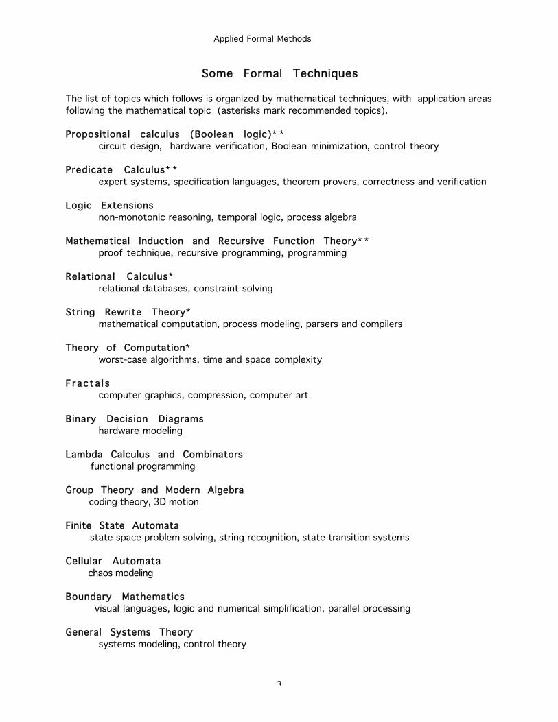
The list of topics which follows is organized by mathematical techniques, with application areas
following the mathematical topic (asterisks mark recommended topics).
Propositional calculus (Boolean logic)* *
circuit design, hardware verification, Boolean minimization, control theory
Predicate Calculus* *
expert systems, specification languages, theorem provers, correctness and verification
Logic Extensions
non-monotonic reasoning, temporal logic, process algebra
Mathematical Induction and Recursive Function Theory* *
proof technique, recursive programming, programming
Relational Calculus*
relational databases, constraint solving
String Rewrite Theory*
mathematical computation, process modeling, parsers and compilers
Theory of Computation*
worst-case algorithms, time and space complexity
F rac ta l s
computer graphics, compression, computer art
Binary Decision Diagrams
hardware modeling
Lambda Calculus and Combinators
functional programming
Group Theory and Modern Algebra
coding theory, 3D motion
Finite State Automata
state space problem solving, string recognition, state transition systems
Cellular Automata
chaos modeling
Boundary Mathematics
visual languages, logic and numerical simplification, parallel processing
General Systems Theory
systems modeling, control theory
Applied Formal Methods
4
Refe rences
Genera l :
Bavel (1982), Math Companion for Computer Science, Prentice-Hall
Gilbert (1976), Modern Algebra with Applications, Wiley
Grassmann and Tremblay (1996), Logic and Discrete Mathematics, Prentice-Hall
Gries and Schneider (1993), A Logical Approach to Discrete Math, Springer-Verlag
Grimaldi (1999), Discrete and Combinatorial Mathematics, Fourth edition, Addison-Wesley
Lucas (1985), Introduction to Abstract Mathematics, Second edition, Ardsley House
Wolfram (1996), The Mathematica Book, Third edition, Cambridge Press
Spec i f i c :
Aho, Sethi and Ullman (1986), Compilers, Addison-Wesley
Barwise and Etchemendy (1993), The Language of First-Order Logic, Third edition, CSLI Stanford
Forbus and DeKleer (1993), Building Problem Solvers, MIT Press
Genesereth and Nilsson (1987), Logical Foundations of Artificial Intelligence, Kauffman
Hopcroft and Ullman (1979), Introduction to Automata Theory, Languages, and Computation,
Addison-Wesley
Lakatos (1976), Proofs and Refutations, Cambridge U. Press
MacLennan (1990), Functional Programming, Practice and Theory, Addison-Wesley
Manna and Waldinger (1985), The Logical Basis for Computer Programming, Addison-Wesley
Plasmeijer and vanEekelen (1993), Functional Programming and Parallel Graph Rewriting,
Addison-Wesley
Wos, Overbeek, Lusk and Boyle (1992), Automated Reasoning, Second edition, McGraw-Hill
Web Pointers
Oxford University Computing Laboratory
http://www.comlab.ox.ac.uk/archive/formal-methods.html
BYU Laboratory for Applied Logic
http://lal.cs.byu.edu/
NASA Langley Research Center Formal Methods Program
http://shemesh.larc.nasa.gov/fm.html
Swedish Institute of Computer Science
http://www.sics.se/fdt/research97.html
UC Davis Programming Languages and Verification Laboratory
http://avalon.cs.ucdavis.edu/
Stanford U. Center for Formal Methods
http://www-formal.stanford.edu/jmc/math.html
Applied Formal Methods
5
Warsaw U. Applied Logic Group
http://zls.mimuw.edu.pl/english.html
UC Berkeley Design Technology Warehouse
http://www-cad.eecs.berkeley.edu/
A Computational Logic
http://www.cs.utexas.edu/users/moore/acl2/acl2-doc.html
Formal Methods in Software Engineering
http://wwwsel.iit.nrc.ca/projects/fm/fm.html
Formal methods around the world
http://lal.cs.byu.edu/other_FM.html
Software Development using Formal Methods Syllabus
http://www.mcs.salford.ac.uk/sdformal.html
Bibliography on software engineering and formal methods
http://bavi.unice.fr/Biblio/SE/Contrib.html
Seven Myths of Formal Methods
http://www.progsoc.uts.edu.au/~geldridg/frsd/ass1/7myths.htm
Formal Methods - selected historical references
http://docs.dcs.napier.ac.uk/DOCS/GET/jones92a/document.html
Books
http://www.rspa.com/spi/formal.html
Applied Formal Methods
6
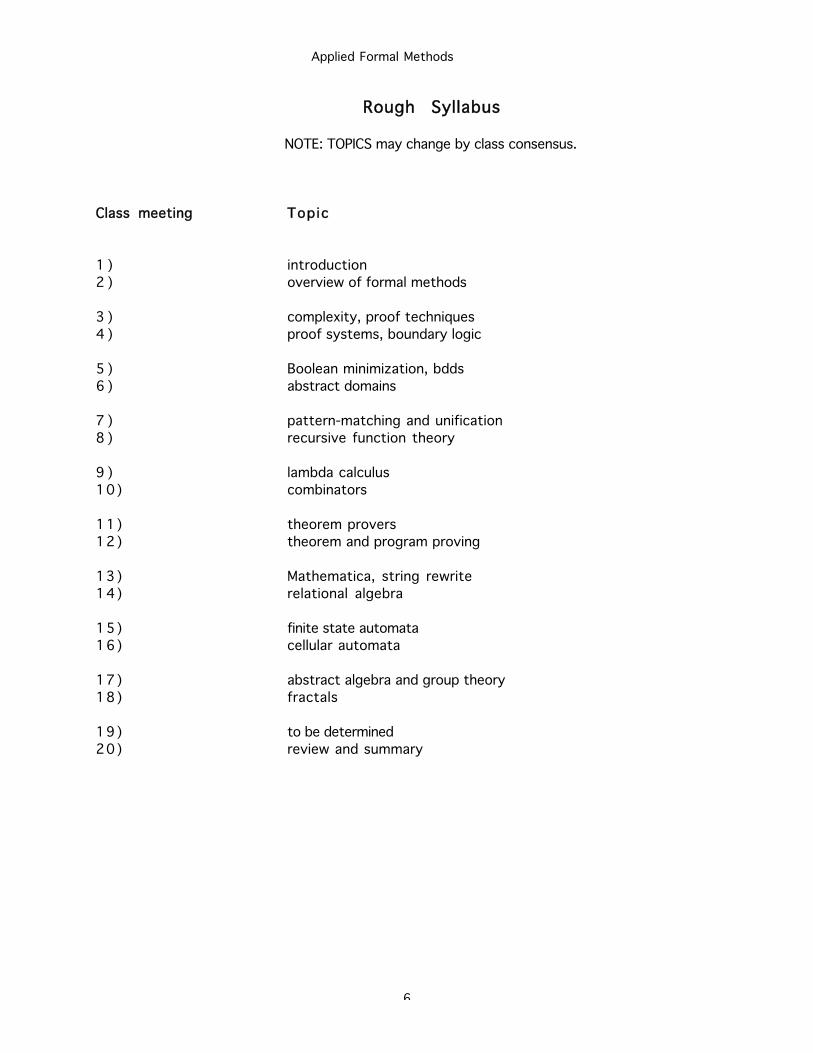
Rough Syllabus
NOTE: TOPICS may change by class consensus.
Class meeting Topic
1 ) introduction
2 ) overview of formal methods
3 ) complexity, proof techniques
4 ) proof systems, boundary logic
5 ) Boolean minimization, bdds
6 ) abstract domains
7 ) pattern-matching and unification
8 ) recursive function theory
9 ) lambda calculus
10) combinators
11) theorem provers
12) theorem and program proving
13) Mathematica, string rewrite
14) relational algebra
15) finite state automata
16) cellular automata
17) abstract algebra and group theory
18) fractals
19) to be determined
20) review and summary
Applied Formal Methods
1
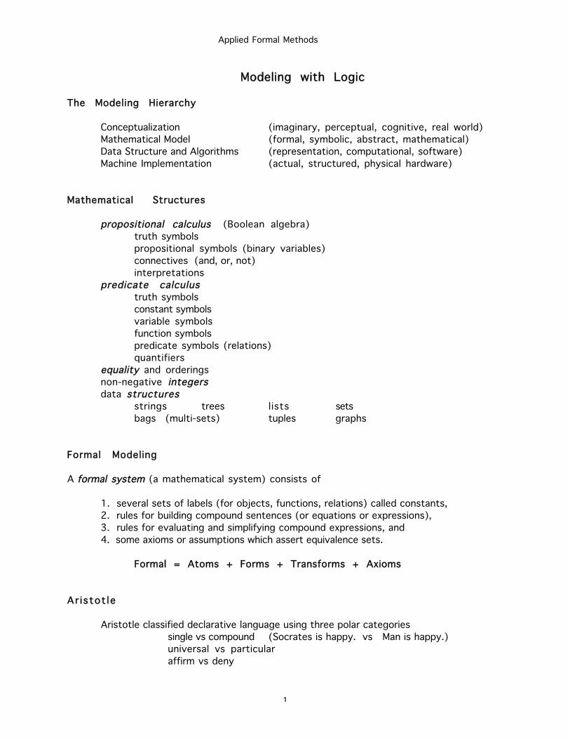
Modeling with Logic
The Modeling Hierarchy
Conceptualization (imaginary, perceptual, cognitive, real world)
Mathematical Model (formal, symbolic, abstract, mathematical)
Data Structure and Algorithms (representation, computational, software)
Machine Implementation (actual, structured, physical hardware)
Mathematical Structures
propositional calculus (Boolean algebra)
truth symbols
propositional symbols (binary variables)
connectives (and, or, not)
interpretations
predicate calculustruth symbols
constant symbols
variable symbols
function symbols
predicate symbols (relations)
quantifiers
equality and orderings
non-negative integersdata structures
strings trees lists sets
bags (multi-sets) tuples graphs
Formal Modeling
A formal system (a mathematical system) consists of
1. several sets of labels (for objects, functions, relations) called constants,
2. rules for building compound sentences (or equations or expressions),
3. rules for evaluating and simplifying compound expressions, and
4. some axioms or assumptions which assert equivalence sets.
Formal = Atoms + Forms + Transforms + Axioms
Ar istot le
Aristotle classified declarative language using three polar categories
single vs compound (Socrates is happy. vs Man is happy.)
universal vs particular
affirm vs deny
Applied Formal Methods
2
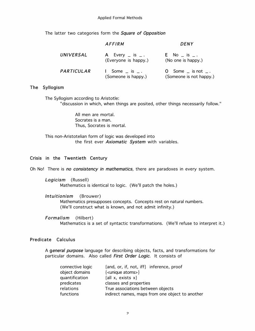
The latter two categories form the Square of Opposition
A F F I R M DENY
UNIVERSAL A Every _ is _ . EE No _ is _ .
(Everyone is happy.) (No one is happy.)
PARTICULAR I Some _ is _ . OO Some _ is not _ .
(Someone is happy.) (Someone is not happy.)
The Syllogism
The Syllogism according to Aristotle:
"discussion in which, when things are posited, other things necessarily follow."
All men are mortal.
Socrates is a man.
Thus, Socrates is mortal.
This non-Aristotelian form of logic was developed into
the first ever Axiomatic System with variables.
Crisis in the Twentieth Century
Oh No! There is no consistency in mathematics, there are paradoxes in every system.
Logicism (Russell)
Mathematics is identical to logic. (We'll patch the holes.)
Intuitionism (Brouwer)
Mathematics presupposes concepts. Concepts rest on natural numbers.
(We'll construct what is known, and not admit infinity.)
Formal ism (Hilbert)
Mathematics is a set of syntactic transformations. (We'll refuse to interpret it.)
Predicate Calculus
A ggeneral purpose language for describing objects, facts, and transformations for
particular domains. Also called First Order Logic. It consists of
connective logic {and, or, if, not, iff} inference, proof
object domains {<unique atoms>}
quantification {all x, exists x}
predicates classes and properties
relations True associations between objects
functions indirect names, maps from one object to another
Applied Formal Methods
3
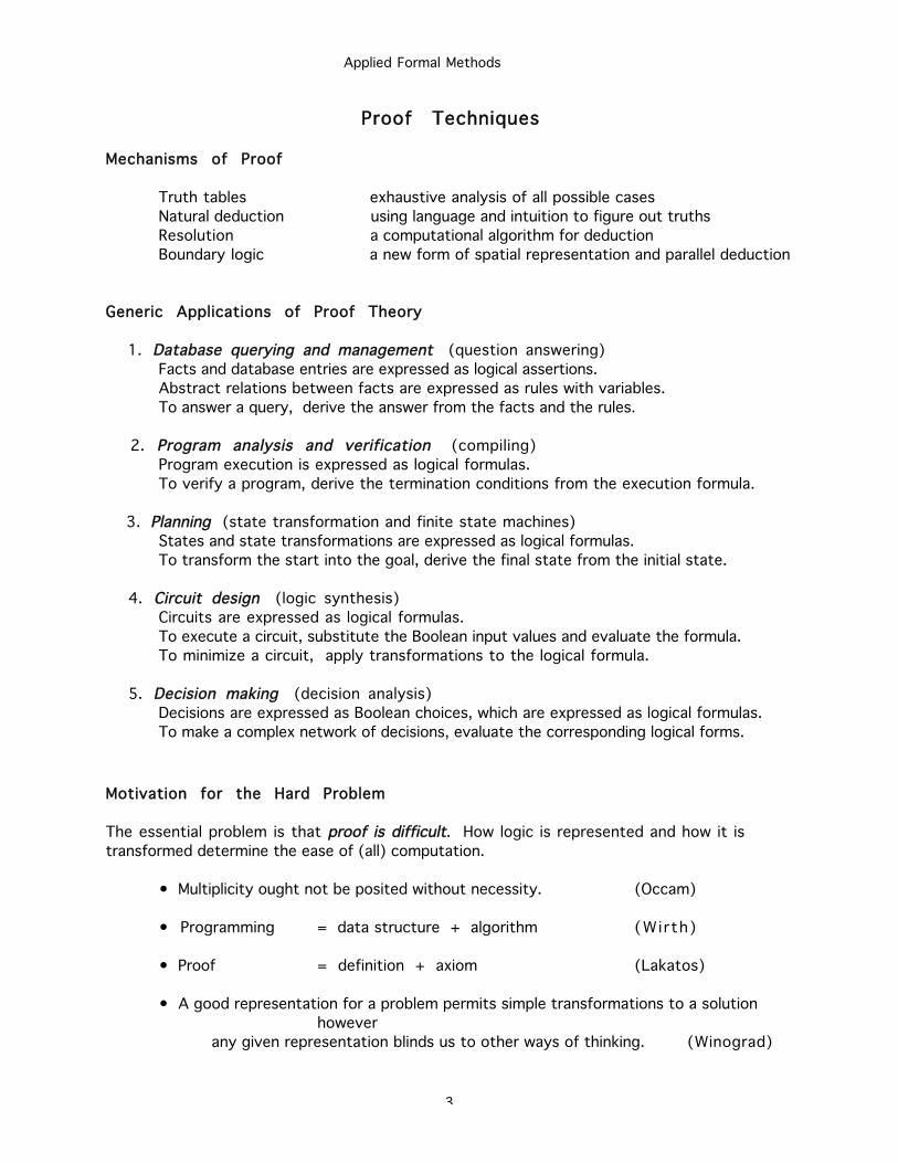
Proof Techniques
Mechanisms of Proof
Truth tables exhaustive analysis of all possible cases
Natural deduction using language and intuition to figure out truths
Resolution a computational algorithm for deduction
Boundary logic a new form of spatial representation and parallel deduction
Generic Applications of Proof Theory
1. Database querying and management (question answering)
Facts and database entries are expressed as logical assertions.
Abstract relations between facts are expressed as rules with variables.
To answer a query, derive the answer from the facts and the rules.
2. Program analysis and verification (compiling)
Program execution is expressed as logical formulas.
To verify a program, derive the termination conditions from the execution formula.
3. PPlanning (state transformation and finite state machines)
States and state transformations are expressed as logical formulas.
To transform the start into the goal, derive the final state from the initial state.
4. Circuit design (logic synthesis)
Circuits are expressed as logical formulas.
To execute a circuit, substitute the Boolean input values and evaluate the formula.
To minimize a circuit, apply transformations to the logical formula.
5. DDecision making (decision analysis)
Decisions are expressed as Boolean choices, which are expressed as logical formulas.
To make a complex network of decisions, evaluate the corresponding logical forms.
Motivation for the Hard Problem
The essential problem is that proof is difficult. How logic is represented and how it is
transformed determine the ease of (all) computation.
• Multiplicity ought not be posited without necessity. (Occam)
• Programming = data structure + algorithm (Wirth)
• Proof = definition + axiom (Lakatos)
• A good representation for a problem permits simple transformations to a solution
however
any given representation blinds us to other ways of thinking. (Winograd)
Applied Formal Methods
4
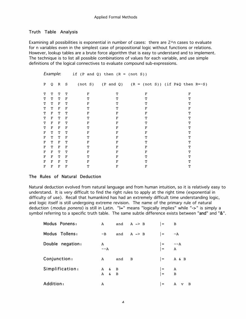
Truth Table Analysis
Examining all possibilities is exponential in number of cases: there are 2^n cases to evaluate
for n variables even in the simplest case of propositional logic without functions or relations.
However, lookup tables are a brute force algorithm that is easy to understand and to implement.
The technique is to list all possible combinations of values for each variable, and use simple
definitions of the logical connectives to evaluate compound sub-expressions.
Example: if (P and Q) then (R = (not S))
P Q R S (not S) (P and Q) (R = (not S)) (if P&Q then R=~S)
T T T T F T F FT T T F T T T TT T F T F T T TT T F F T T F FT F T T F F F TT F T F T F T TT F F T F F T TT F F F T F F TF T T T F F F TF T T F T F T TF T F T F F T TF T F F T F F TF F T T F F F TF F T F T F T TF F F T F F T TF F F F T F F T
The Rules of Natural Deduction
Natural deduction evolved from natural language and from human intuition, so it is relatively easy to
understand. It is very difficult to find the right rules to apply at the right time (exponential in
difficulty of use). Recall that humankind has had an extremely difficult time understanding logic,
and logic itself is still undergoing extreme revision. The name of the primary rule of natural
deduction (modus ponens) is still in Latin. "||=" means "logically implies" while "-->" is simply a
symbol referring to a specific truth table. The same subtle difference exists between "aand" and "&&".
Modus Ponens: A and A -> B |= B
Modus Tollens: ~B and A -> B |= ~A
Double negation: A |= ~~A~~A |= A
Conjunction: A and B |= A & B
S imp l i f i cat ion: A & B |= AA & B |= B
Addition: A |= A v B
Applied Formal Methods
5
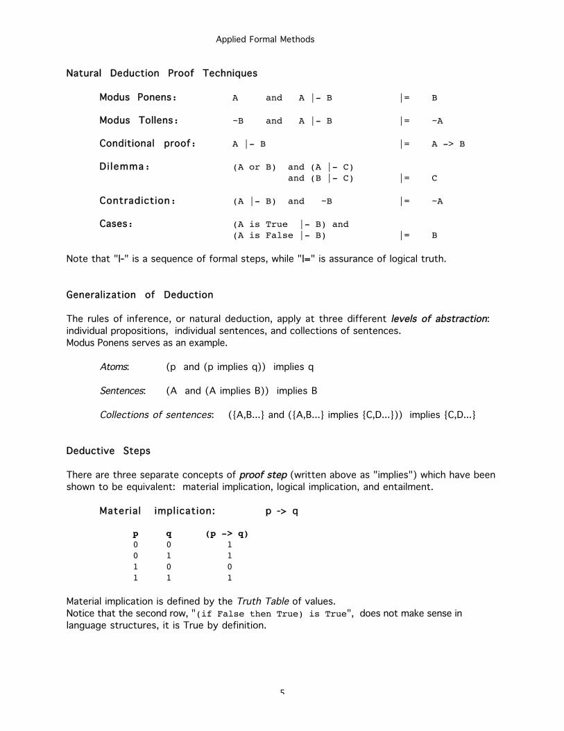
Natural Deduction Proof Techniques
Modus Ponens: A and A |- B |= B
Modus Tollens: ~B and A |- B |= ~A
Conditional proof: A |- B |= A -> B
Di lemma: (A or B) and (A |- C) and (B |- C) |= C
Contradiction: (A |- B) and ~B |= ~A
Cases: (A is True |- B) and(A is False |- B) |= B
Note that "||-" is a sequence of formal steps, while "||=" is assurance of logical truth.
Generalization of Deduction
The rules of inference, or natural deduction, apply at three different levels of abstraction:
individual propositions, individual sentences, and collections of sentences.
Modus Ponens serves as an example.
Atoms: (p and (p implies q)) implies q
Sentences: (A and (A implies B)) implies B
Collections of sentences: ({A,B...} and ({A,B...} implies {C,D...})) implies {C,D...}
Deductive Steps
There are three separate concepts of proof step (written above as "implies") which have been
shown to be equivalent: material implication, logical implication, and entailment.
Material impl ication: p -> q
p q (p -> q)0 0 10 1 11 0 01 1 1
Material implication is defined by the Truth Table of values.
Notice that the second row, "(if False then True) is True", does not make sense in
language structures, it is True by definition.
Applied Formal Methods
6
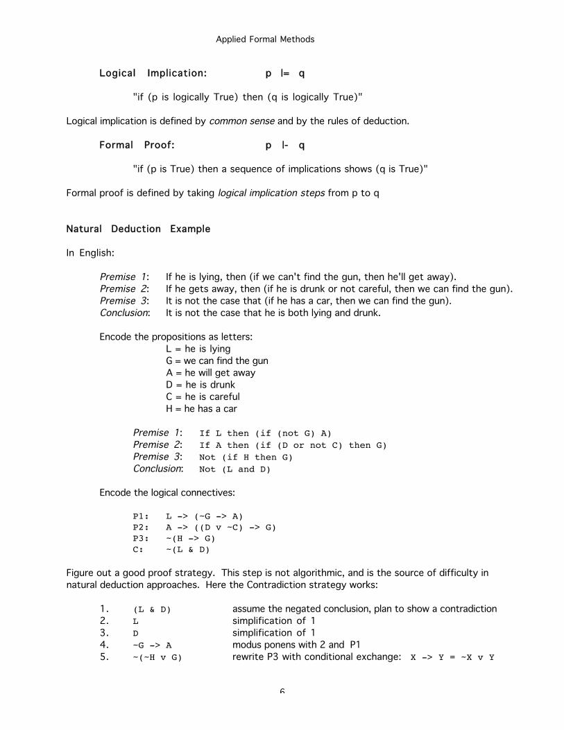
Logical Implication: p |= q
"if (p is logically True) then (q is logically True)"
Logical implication is defined by common sense and by the rules of deduction.
Formal Proof: p |- q
"if (p is True) then a sequence of implications shows (q is True)"
Formal proof is defined by taking logical implication steps from p to q
Natural Deduction Example
In English:
Premise 1: If he is lying, then (if we can't find the gun, then he'll get away).
Premise 2: If he gets away, then (if he is drunk or not careful, then we can find the gun).
Premise 3: It is not the case that (if he has a car, then we can find the gun).
Conclusion: It is not the case that he is both lying and drunk.
Encode the propositions as letters:
L = he is lying
G = we can find the gun
A = he will get away
D = he is drunk
C = he is careful
H = he has a car
Premise 1: If L then (if (not G) A)Premise 2: If A then (if (D or not C) then G)Premise 3: Not (if H then G)Conclusion: Not (L and D)
Encode the logical connectives:
P1: L -> (~G -> A)P2: A -> ((D v ~C) -> G)P3: ~(H -> G)C: ~(L & D)
Figure out a good proof strategy. This step is not algorithmic, and is the source of difficulty in
natural deduction approaches. Here the Contradiction strategy works:
1. (L & D) assume the negated conclusion, plan to show a contradiction
2. L simplification of 1
3. D simplification of 1
4. ~G -> A modus ponens with 2 and P1
5. ~(~H v G) rewrite P3 with conditional exchange: X -> Y = ~X v Y
Applied Formal Methods
7
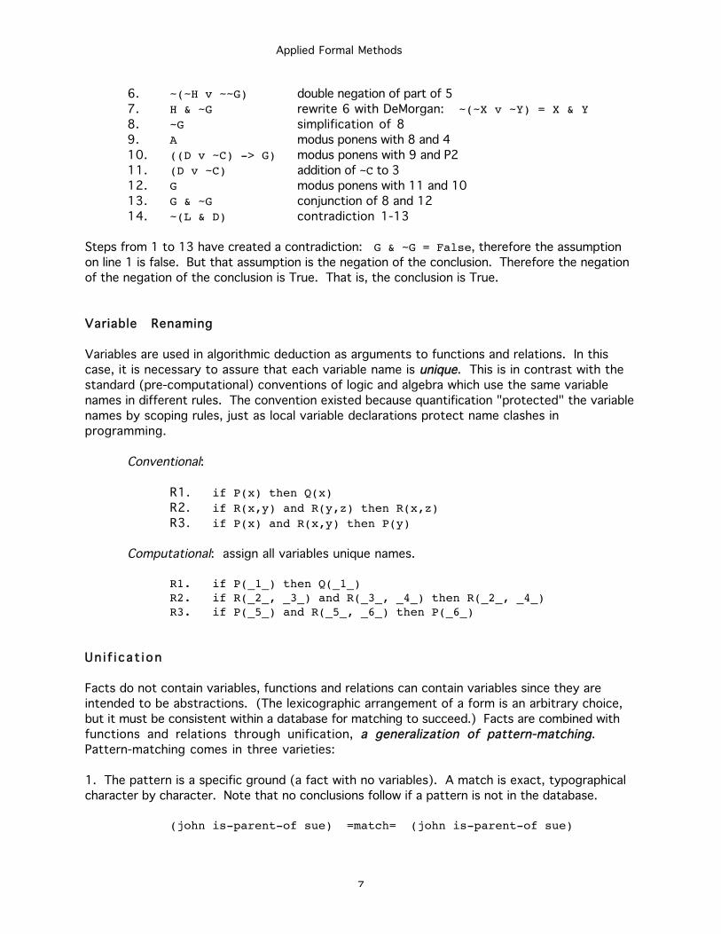
6. ~(~H v ~~G) double negation of part of 5
7. H & ~G rewrite 6 with DeMorgan: ~(~X v ~Y) = X & Y8. ~G simplification of 8
9. A modus ponens with 8 and 4
10. ((D v ~C) -> G) modus ponens with 9 and P2
11. (D v ~C) addition of ~C to 3
12. G modus ponens with 11 and 10
13. G & ~G conjunction of 8 and 12
14. ~(L & D) contradiction 1-13
Steps from 1 to 13 have created a contradiction: G & ~G = False, therefore the assumption
on line 1 is false. But that assumption is the negation of the conclusion. Therefore the negation
of the negation of the conclusion is True. That is, the conclusion is True.
Variable Renaming
Variables are used in algorithmic deduction as arguments to functions and relations. In this
case, it is necessary to assure that each variable name is unique. This is in contrast with the
standard (pre-computational) conventions of logic and algebra which use the same variable
names in different rules. The convention existed because quantification "protected" the variable
names by scoping rules, just as local variable declarations protect name clashes in
programming.
Conventional:
R1. if P(x) then Q(x)R2. if R(x,y) and R(y,z) then R(x,z)R3. if P(x) and R(x,y) then P(y)
Computational: assign all variables unique names.
R1. if P(_1_) then Q(_1_)R2. if R(_2_, _3_) and R(_3_, _4_) then R(_2_, _4_)R3. if P(_5_) and R(_5_, _6_) then P(_6_)
Un i f i ca t ion
Facts do not contain variables, functions and relations can contain variables since they are
intended to be abstractions. (The lexicographic arrangement of a form is an arbitrary choice,
but it must be consistent within a database for matching to succeed.) Facts are combined with
functions and relations through unification, a generalization of pattern-matching.
Pattern-matching comes in three varieties:
1. The pattern is a specific ground (a fact with no variables). A match is exact, typographical
character by character. Note that no conclusions follow if a pattern is not in the database.
(john is-parent-of sue) =match= (john is-parent-of sue)
Applied Formal Methods
8
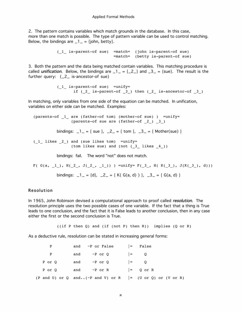
2. The pattern contains variables which match grounds in the database. In this case,
more than one match is possible. The type of pattern variable can be used to control matching.
Below, the bindings are _1_ = {john, betty}.
(_1_ is-parent-of sue) =match= (john is-parent-of sue) =match= (betty is-parent-of sue)
3. Both the pattern and the data being matched contain variables. This matching procedure is
called unification. Below, the bindings are _1_ = {_2_} and _3_ = {sue}. The result is the
further query: (_2_ is-ancestor-of sue)
(_1_ is-parent-of sue) =unify= if (_2_ is-parent-of _3_) then (_2_ is-ancestor-of _3_)
In matching, only variables from one side of the equation can be matched. In unification,
variables on either side can be matched. Examples:
(parents-of _1_ are (father-of tom) (mother-of sue) ) =unify=(parents-of sue are (father-of _2_) _3_)
bindings: _1_ = { sue }, _2_ = { tom }, _3_ = { Mother(sue) }
(_1_ likes _2_) and (sue likes tom) =unify=(tom likes sue) and (not (_3_ likes _4_))
bindings: fail. The word "not" does not match.
F( G(a, _1_), H(_2_, J(_2_, _1_)) ) =unify= F(_3_, H( K(_3_), J(K(_3_), d)))
bindings: _1_ = {d}, _2_ = { K( G(a, d) ) }, _3_ = { G(a, d) }
Reso lut ion
In 1965, John Robinson devised a computational approach to proof called resolution. The
resolution principle uses the two possible cases of one variable. If the fact that a thing is True
leads to one conclusion, and the fact that it is False leads to another conclusion, then in any case
either the first or the second conclusion is True.
((if P then Q) and (if (not P) then R)) implies (Q or R)
As a deductive rule, resolution can be stated in increasing general forms:
P and ~P or False |= False
P and ~P or Q |= Q
P or Q and ~P or Q |= Q
P or Q and ~P or R |= Q or R
(P and U) or Q and..(~P and V) or R |= (U or Q) or (V or R)
Applied Formal Methods
9
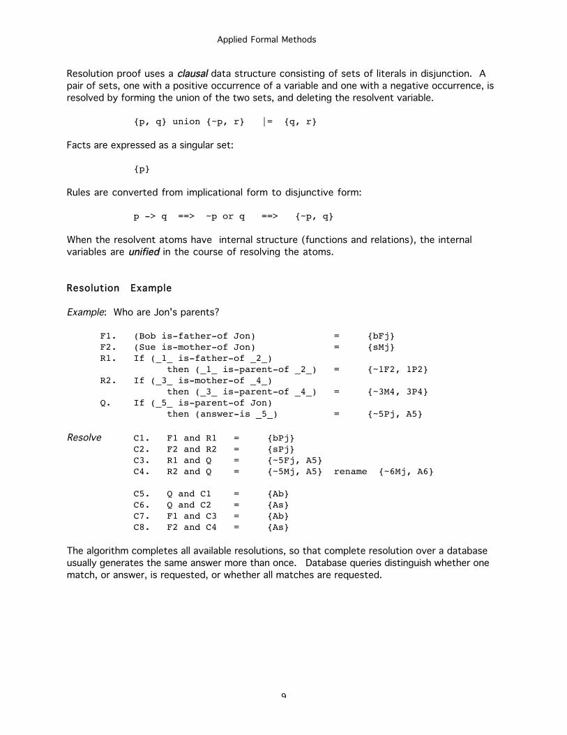
Resolution proof uses a clausal data structure consisting of sets of literals in disjunction. A
pair of sets, one with a positive occurrence of a variable and one with a negative occurrence, is
resolved by forming the union of the two sets, and deleting the resolvent variable.
{p, q} union {~p, r} |= {q, r}
Facts are expressed as a singular set:
{p}
Rules are converted from implicational form to disjunctive form:
p -> q ==> ~p or q ==> {~p, q}
When the resolvent atoms have internal structure (functions and relations), the internal
variables are unified in the course of resolving the atoms.
Resolution Example
Example: Who are Jon's parents?
F1. (Bob is-father-of Jon) = {bFj}F2. (Sue is-mother-of Jon) = {sMj}R1. If (_1_ is-father-of _2_)
then (_1_ is-parent-of _2_) = {~1F2, 1P2}R2. If (_3_ is-mother-of _4_)
then (_3_ is-parent-of _4_) = {~3M4, 3P4}Q. If (_5_ is-parent-of Jon)
then (answer-is _5_) = {~5Pj, A5}
Resolve C1. F1 and R1 = {bPj}C2. F2 and R2 = {sPj}C3. R1 and Q = {~5Fj, A5}C4. R2 and Q = {~5Mj, A5} rename {~6Mj, A6}
C5. Q and C1 = {Ab}C6. Q and C2 = {As}C7. F1 and C3 = {Ab}C8. F2 and C4 = {As}
The algorithm completes all available resolutions, so that complete resolution over a database
usually generates the same answer more than once. Database queries distinguish whether one
match, or answer, is requested, or whether all matches are requested.
Applied Formal Methods
10
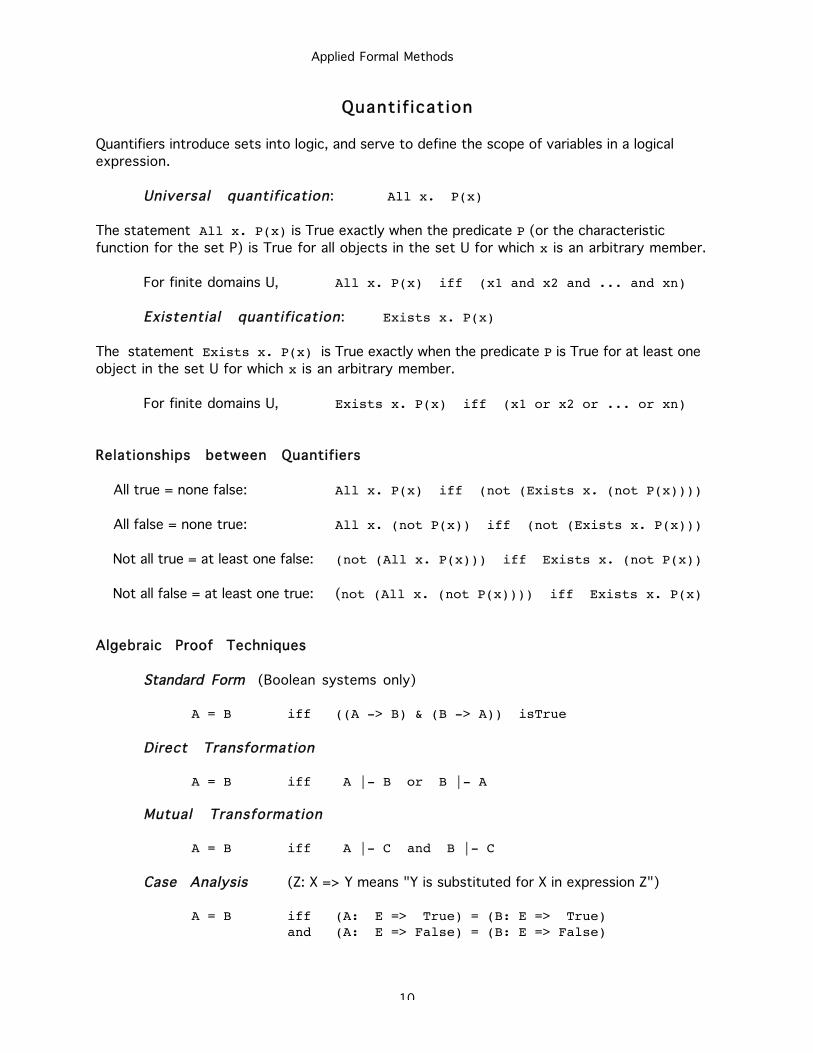
Quantif icat ion
Quantifiers introduce sets into logic, and serve to define the scope of variables in a logical
expression.
Universal quantification: All x. P(x)
The statement All x. P(x) is True exactly when the predicate P (or the characteristic
function for the set P) is True for all objects in the set U for which x is an arbitrary member.
For finite domains U, All x. P(x) iff (x1 and x2 and ... and xn)
Existential quantification: Exists x. P(x)
The statement Exists x. P(x) is True exactly when the predicate P is True for at least one
object in the set U for which x is an arbitrary member.
For finite domains U, Exists x. P(x) iff (x1 or x2 or ... or xn)
Relationships between Quantifiers
All true = none false: All x. P(x) iff (not (Exists x. (not P(x))))
All false = none true: All x. (not P(x)) iff (not (Exists x. P(x)))
Not all true = at least one false: (not (All x. P(x))) iff Exists x. (not P(x))
Not all false = at least one true: (not (All x. (not P(x)))) iff Exists x. P(x)
Algebraic Proof Techniques
Standard Form (Boolean systems only)
A = B iff ((A -> B) & (B -> A)) isTrue
Direct Transformation
A = B iff A |- B or B |- A
Mutual Transformation
A = B iff A |- C and B |- C
Case Analysis (Z: X => Y means "Y is substituted for X in expression Z")
A = B iff (A: E => True) = (B: E => True)and (A: E => False) = (B: E => False)
Applied Formal Methods
11
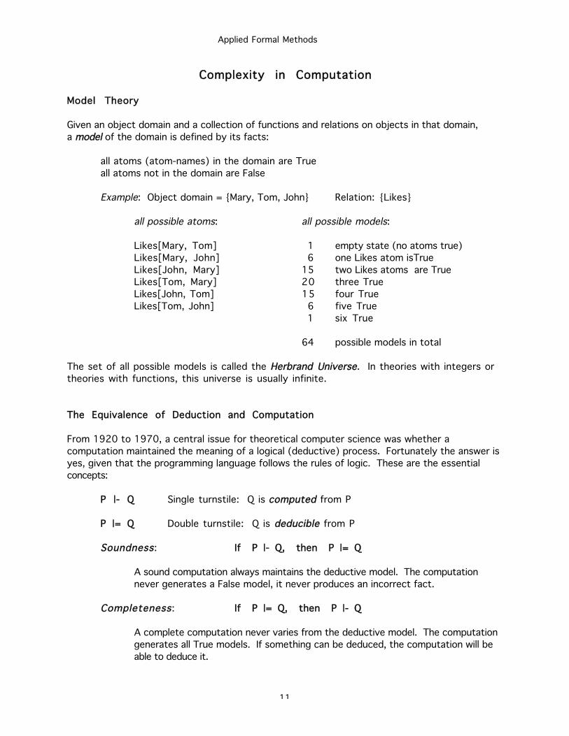
Complexity in Computation
Model Theory
Given an object domain and a collection of functions and relations on objects in that domain,
a model of the domain is defined by its facts:
all atoms (atom-names) in the domain are True
all atoms not in the domain are False
Example: Object domain = {Mary, Tom, John} Relation: {Likes}
all possible atoms: all possible models:
Likes[Mary, Tom] 1 empty state (no atoms true)
Likes[Mary, John] 6 one Likes atom isTrue
Likes[John, Mary] 15 two Likes atoms are True
Likes[Tom, Mary] 20 three True
Likes[John, Tom] 15 four True
Likes[Tom, John] 6 five True
1 six True
64 possible models in total
The set of all possible models is called the Herbrand Universe. In theories with integers or
theories with functions, this universe is usually infinite.
The Equivalence of Deduction and Computation
From 1920 to 1970, a central issue for theoretical computer science was whether a
computation maintained the meaning of a logical (deductive) process. Fortunately the answer is
yes, given that the programming language follows the rules of logic. These are the essential
concepts:
P |- Q Single turnstile: Q is ccomputed from P
P |= Q Double turnstile: Q is deducible from P
Soundness: IIf P |- Q, then P |= Q
A sound computation always maintains the deductive model. The computation
never generates a False model, it never produces an incorrect fact.
Completeness: IIf P |= Q, then P |- Q
A complete computation never varies from the deductive model. The computation
generates all True models. If something can be deduced, the computation will be
able to deduce it.
Applied Formal Methods
12
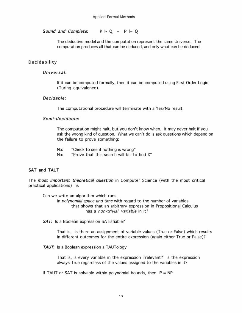
Sound and Complete: PP |- Q = P |= Q
The deductive model and the computation represent the same Universe. The
computation produces all that can be deduced, and only what can be deduced.
Dec idab i l i t y
Un i ve r sa l :
If it can be computed formally, then it can be computed using First Order Logic
(Turing equivalence).
Decidable:
The computational procedure will terminate with a Yes/No result.
Semi-dec idab le :
The computation might halt, but you don't know when. It may never halt if you
ask the wrong kind of question. What we can't do is ask questions which depend on
the ffailure to prove something:
No: "Check to see if nothing is wrong"
No: "Prove that this search will fail to find X"
SAT and TAUT
The most important theoretical question in Computer Science (with the most critical
practical applications) is
Can we write an algorithm which runs
in polynomial space and time with regard to the number of variables
that shows that an arbitrary expression in Propositional Calculus
has a non-trivial variable in it?
SAT: Is a Boolean expression SATisfiable?
That is, is there an assignment of variable values (True or False) which results
in different outcomes for the entire expression (again either True or False)?
TAUT: Is a Boolean expression a TAUTology
That is, is every variable in the expression irrelevant? Is the expression
always True regardless of the values assigned to the variables in it?
If TAUT or SAT is solvable within polynomial bounds, then PP = NP
Applied Formal Methods
13
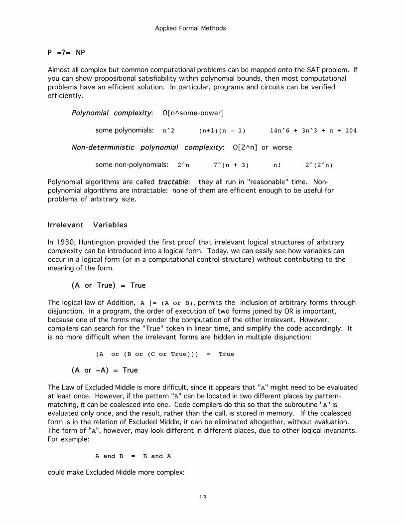
P =?= NP
Almost all complex but common computational problems can be mapped onto the SAT problem. If
you can show propositional satisfiability within polynomial bounds, then most computational
problems have an efficient solution. In particular, programs and circuits can be verified
efficiently.
Polynomial complexity: O[n^some-power]
some polynomials: n^2 (n+1)(n - 1) 14n^6 + 3n^3 + n + 104
Non-deterministic polynomial complexity: O[2^n] or worse
some non-polynomials: 2^n 7^(n + 3) n! 2^(2^n)
Polynomial algorithms are called tractable: they all run in "reasonable" time. Non-
polynomial algorithms are intractable: none of them are efficient enough to be useful for
problems of arbitrary size.
Irrelevant Variables
In 1930, Huntington provided the first proof that irrelevant logical structures of arbitrary
complexity can be introduced into a logical form. Today, we can easily see how variables can
occur in a logical form (or in a computational control structure) without contributing to the
meaning of the form.
(A or True) = True
The logical law of Addition, A |= (A or B), permits the inclusion of arbitrary forms through
disjunction. In a program, the order of execution of two forms joined by OR is important,
because one of the forms may render the computation of the other irrelevant. However,
compilers can search for the "True" token in linear time, and simplify the code accordingly. It
is no more difficult when the irrelevant forms are hidden in multiple disjunction:
(A or (B or (C or True))) = True
(A or ~A) = True
The Law of Excluded Middle is more difficult, since it appears that "A" might need to be evaluated
at least once. However, if the pattern "A" can be located in two different places by pattern-
matching, it can be coalesced into one. Code compilers do this so that the subroutine "A" is
evaluated only once, and the result, rather than the call, is stored in memory. If the coalesced
form is in the relation of Excluded Middle, it can be eliminated altogether, without evaluation.
The form of "A", however, may look different in different places, due to other logical invariants.
For example:
A and B = B and A
could make Excluded Middle more complex:
Applied Formal Methods
14
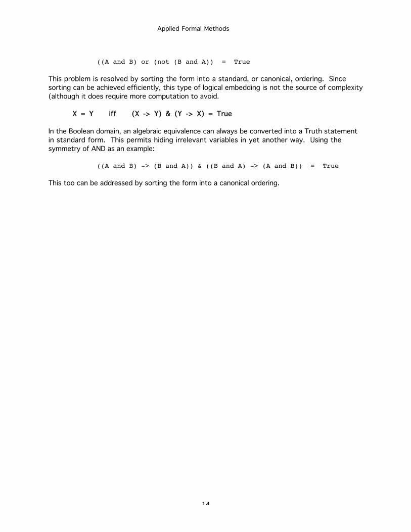
((A and B) or (not (B and A)) = True
This problem is resolved by sorting the form into a standard, or canonical, ordering. Since
sorting can be achieved efficiently, this type of logical embedding is not the source of complexity
(although it does require more computation to avoid.
X = Y iff (X -> Y) & (Y -> X) = True
In the Boolean domain, an algebraic equivalence can always be converted into a Truth statement
in standard form. This permits hiding irrelevant variables in yet another way. Using the
symmetry of AND as an example:
((A and B) -> (B and A)) & ((B and A) -> (A and B)) = True
This too can be addressed by sorting the form into a canonical ordering.
Applied Formal Methods
15
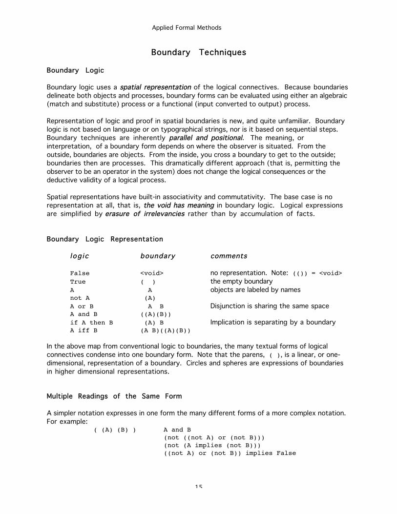
Boundary Techniques
Boundary Logic
Boundary logic uses a spatial representation of the logical connectives. Because boundaries
delineate both objects and processes, boundary forms can be evaluated using either an algebraic
(match and substitute) process or a functional (input converted to output) process.
Representation of logic and proof in spatial boundaries is new, and quite unfamiliar. Boundary
logic is not based on language or on typographical strings, nor is it based on sequential steps.
Boundary techniques are inherently parallel and positional. The meaning, or
interpretation, of a boundary form depends on where the observer is situated. From the
outside, boundaries are objects. From the inside, you cross a boundary to get to the outside;
boundaries then are processes. This dramatically different approach (that is, permitting the
observer to be an operator in the system) does not change the logical consequences or the
deductive validity of a logical process.
Spatial representations have built-in associativity and commutativity. The base case is no
representation at all, that is, the void has meaning in boundary logic. Logical expressions
are simplified by erasure of irrelevancies rather than by accumulation of facts.
Boundary Logic Representation
log i c boundary comments
False <void> no representation. Note: (()) = <void>True ( ) the empty boundary
A A objects are labeled by namesnot A (A)A or B A B Disjunction is sharing the same spaceA and B ((A)(B))if A then B (A) B Implication is separating by a boundaryA iff B (A B)((A)(B))
In the above map from conventional logic to boundaries, the many textual forms of logical
connectives condense into one boundary form. Note that the parens, ( ), is a linear, or one-
dimensional, representation of a boundary. Circles and spheres are expressions of boundaries
in higher dimensional representations.
Multiple Readings of the Same Form
A simpler notation expresses in one form the many different forms of a more complex notation.
For example:( (A) (B) ) A and B
(not ((not A) or (not B)))(not (A implies (not B)))((not A) or (not B)) implies False
Applied Formal Methods
16
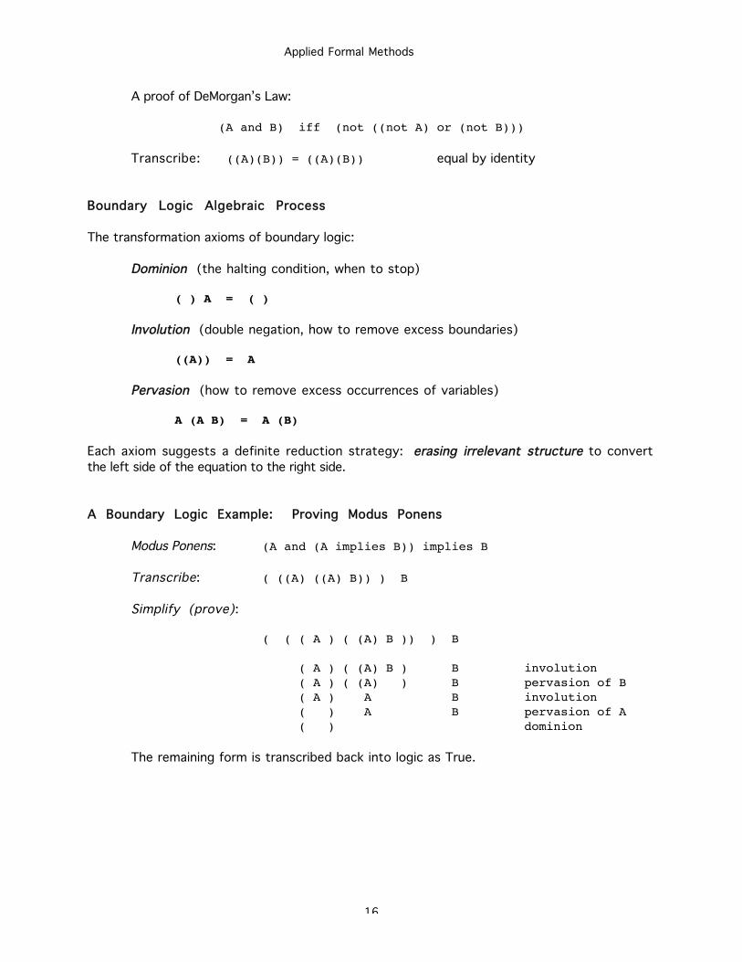
A proof of DeMorgan’s Law:
(A and B) iff (not ((not A) or (not B)))
Transcribe: ((A)(B)) = ((A)(B)) equal by identity
Boundary Logic Algebraic Process
The transformation axioms of boundary logic:
Dominion (the halting condition, when to stop)
( ) A = ( )
Involution (double negation, how to remove excess boundaries)
((A)) = A
Pervasion (how to remove excess occurrences of variables)
A (A B) = A (B)
Each axiom suggests a definite reduction strategy: eerasing irrelevant structure to convert
the left side of the equation to the right side.
A Boundary Logic Example: Proving Modus Ponens
Modus Ponens: (A and (A implies B)) implies B
Transcribe: ( ((A) ((A) B)) ) B
Simplify (prove):
( ( ( A ) ( (A) B )) ) B
( A ) ( (A) B ) B involution ( A ) ( (A) ) B pervasion of B ( A ) A B involution ( ) A B pervasion of A ( ) dominion
The remaining form is transcribed back into logic as True.
Applied Formal Methods
17
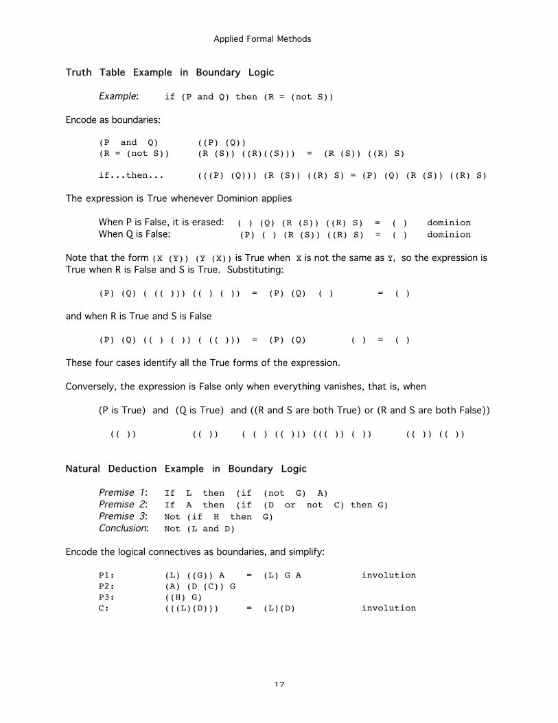
Truth Table Example in Boundary Logic
Example: if (P and Q) then (R = (not S))
Encode as boundaries:
(P and Q) ((P) (Q))(R = (not S)) (R (S)) ((R)((S))) = (R (S)) ((R) S)
if...then... (((P) (Q))) (R (S)) ((R) S) = (P) (Q) (R (S)) ((R) S)
The expression is True whenever Dominion applies
When P is False, it is erased: ( ) (Q) (R (S)) ((R) S) = ( ) dominionWhen Q is False: (P) ( ) (R (S)) ((R) S) = ( ) dominion
Note that the form (X (Y)) (Y (X)) is True when X is not the same as Y, so the expression is
True when R is False and S is True. Substituting:
(P) (Q) ( (( ))) (( ) ( )) = (P) (Q) ( ) = ( )
and when R is True and S is False
(P) (Q) (( ) ( )) ( (( ))) = (P) (Q) ( ) = ( )
These four cases identify all the True forms of the expression.
Conversely, the expression is False only when everything vanishes, that is, when
(P is True) and (Q is True) and ((R and S are both True) or (R and S are both False))
(( )) (( )) ( ( ) (( ))) ((( )) ( )) (( )) (( ))
Natural Deduction Example in Boundary Logic
Premise 1: If L then (if (not G) A)Premise 2: If A then (if (D or not C) then G)Premise 3: Not (if H then G)Conclusion: Not (L and D)
Encode the logical connectives as boundaries, and simplify:
P1: (L) ((G)) A = (L) G A involutionP2: (A) (D (C)) GP3: ((H) G)C: (((L)(D))) = (L)(D) involution
Applied Formal Methods
18
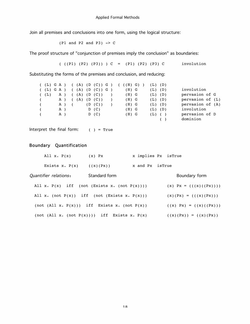
Join all premises and conclusions into one form, using the logical structure:
(P1 and P2 and P3) -> C
The proof structure of "conjunction of premises imply the conclusion" as boundaries:
( ((P1) (P2) (P3)) ) C = (P1) (P2) (P3) C involution
Substituting the forms of the premises and conclusion, and reducing:
( (L) G A ) ( (A) (D (C)) G ) ( ((H) G) ) (L) (D) ( (L) G A ) ( (A) (D (C)) G ) (H) G (L) (D) involution ( (L) A ) ( (A) (D (C)) ) (H) G (L) (D) pervasion of G ( A ) ( (A) (D (C)) ) (H) G (L) (D) pervasion of (L) ( A ) ( (D (C)) ) (H) G (L) (D) pervasion of (A) ( A ) D (C) (H) G (L) (D) involution ( A ) D (C) (H) G (L) ( ) pervasion of D ( ) dominion
Interpret the final form: ( ) = True
Boundary Quantification
All x. P(x) (x) Px x implies Px isTrue
Exists x. P(x) ((x)(Px)) x and Px isTrue
Quantifier relations: Standard form Boundary form
All x. P(x) iff (not (Exists x. (not P(x)))) (x) Px = (((x)((Px))))
All x. (not P(x)) iff (not (Exists x. P(x))) (x)(Px) = (((x)(Px)))
(not (All x. P(x))) iff Exists x. (not P(x)) ((x) Px) = ((x)((Px)))
(not (All x. (not P(x)))) iff Exists x. P(x) ((x)(Px)) = ((x)(Px))
Applied Formal Methods
1
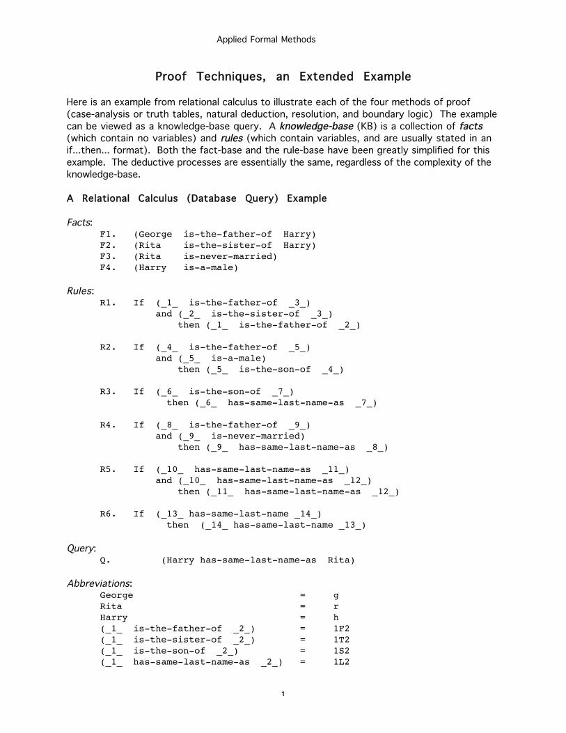
Proof Techniques, an Extended Example
Here is an example from relational calculus to illustrate each of the four methods of proof
(case-analysis or truth tables, natural deduction, resolution, and boundary logic) The example
can be viewed as a knowledge-base query. A knowledge-base (KB) is a collection of facts(which contain no variables) and rules (which contain variables, and are usually stated in an
if...then... format). Both the fact-base and the rule-base have been greatly simplified for this
example. The deductive processes are essentially the same, regardless of the complexity of the
knowledge-base.
A Relational Calculus (Database Query) Example
Facts:F1. (George is-the-father-of Harry)F2. (Rita is-the-sister-of Harry)F3. (Rita is-never-married)F4. (Harry is-a-male)
Rules:R1. If (_1_ is-the-father-of _3_)
and (_2_ is-the-sister-of _3_) then (_1_ is-the-father-of _2_)
R2. If (_4_ is-the-father-of _5_) and (_5_ is-a-male)
then (_5_ is-the-son-of _4_)
R3. If (_6_ is-the-son-of _7_)then (_6_ has-same-last-name-as _7_)
R4. If (_8_ is-the-father-of _9_) and (_9_ is-never-married)
then (_9_ has-same-last-name-as _8_)
R5. If (_10_ has-same-last-name-as _11_) and (_10_ has-same-last-name-as _12_)
then (_11_ has-same-last-name-as _12_)
R6. If (_13_ has-same-last-name _14_)then (_14_ has-same-last-name _13_)
Query:Q. (Harry has-same-last-name-as Rita)
Abbreviations:George = gRita = rHarry = h(_1_ is-the-father-of _2_) = 1F2(_1_ is-the-sister-of _2_) = 1T2
(_1_ is-the-son-of _2_) = 1S2(_1_ has-same-last-name-as _2_) = 1L2
Applied Formal Methods
2
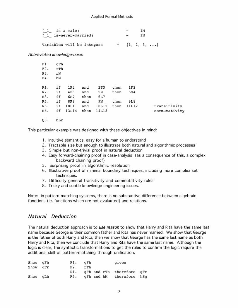
(_1_ is-a-male) = 1M(_1_ is-never-married) = 1N
Variables will be integers = {1, 2, 3, ...}
Abbreviated knowledge-base:
F1. gFhF2. rThF3. rNF4. hM
R1. if 1F3 and 2T3 then 1F2R2. if 4F5 and 5M then 5S4R3. if 6S7 then 6L7R4. if 8F9 and 9N then 9L8R5. if 10L11 and 10L12 then 11L12 transitivityR6. if 13L14 then 14L13 commutativity
Q0. hLr
This particular example was designed with these objectives in mind:
1. Intuitive semantics, easy for a human to understand
2. Tractable size but enough to illustrate both natural and algorithmic processes
3. Simple but non-trivial proof in natural deduction
4. Easy forward-chaining proof in case-analysis (as a consequence of this, a complex
backward chaining proof)
5. Surprising proof in algorithmic resolution
6. Illustrative proof of minimal boundary techniques, including more complex set
techniques.
7. Difficulty general transitivity and commutativity rules
8. Tricky and subtle knowledge engineering issues.
Note: in pattern-matching systems, there is no substantive difference between algebraic
functions (ie. functions which are not evaluated) and relations.
Natural Deduction
The natural deduction approach is to use reason to show that Harry and Rita have the same last
name because George is their common father and Rita has never married. We show that George
is the father of both Harry and Rita, then we show that George has the same last name as both
Harry and Rita, then we conclude that Harry and Rita have the same last name. Although the
logic is clear, the syntactic transformations to get the rules to confirm the logic require the
additional skill of pattern-matching through unification.
Show gFh F1. gFh givenShow gFr F2. rTh
R1. gFh and rTh therefore gFrShow gLh R3. gFh and hM therefore hSg
Applied Formal Methods
3
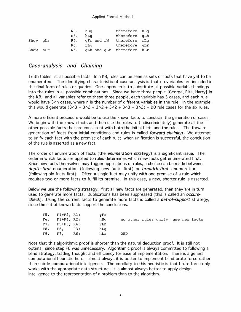
R3. hSg therefore hLgR6. hLg therefore gLh
Show gLr R4. gFr and rN therefore rLgR6. rLg therefore gLr
Show hLr R5. gLh and gLr therefore hLr
Case-analysis and Chaining
Truth tables list all possible facts. In a KB, rules can be seen as sets of facts that have yet to be
enumerated. The identifying characteristic of case-analysis is that no variables are included in
the final form of rules or queries. One approach is to substitute all possible variable bindings
into the rules in all possible combinations. Since we have three people {George, Rita, Harry} in
the KB, and all variables refer to these three people, each variable has 3 cases, and each rule
would have 3^n cases, where n is the number of different variables in the rule. In the example,
this would generate (3^3 + 3^2 + 3^2 + 3^2 + 3^3 + 3^2) = 90 rule cases for the six rules.
A more efficient procedure would be to use the known facts to constrain the generation of cases.
We begin with the known facts and then use the rules to (indiscriminately) generate all the
other possible facts that are consistent with both the initial facts and the rules. The forward
generation of facts from initial conditions and rules is called forward-chaining. We attempt
to unify each fact with the premise of each rule; when unification is successful, the conclusion
of the rule is asserted as a new fact.
The order of enumeration of facts (the enumeration strategy) is a significant issue. The
order in which facts are applied to rules determines which new facts get enumerated first.
Since new facts themselves may trigger applications of rules, a choice can be made between
depth-first enumeration (following new facts first) or breadth-first enumeration
(following old facts first). Often a single fact may unify with one premise of a rule which
requires two or more facts to fulfill its premise. In this case, a new, shorter rule is asserted.
Below we use the following strategy: first all new facts are generated, then they are in turn
used to generate more facts. Duplications has been suppressed (this is called an occurs-check). Using the current facts to generate more facts is called a sset-of-support strategy,
since the set of known facts support the conclusions.
F5. F1+F2, R1: gFrF6. F1+F4, R2: hSg no other rules unify, use new factsF7. F5+F3, R4: rLhF8. F6, R3: hLgF9. F7, R6: hLr QED
Note that this algorithmic proof is shorter than the natural deduction proof. It is still not
optimal, since step F8 was unnecessary. Algorithmic proof is always committed to following a
blind strategy, trading thought and efficiency for ease of implementation. There is a general
computational heuristic here: almost always it is better to implement blind brute force rather
than subtle computational intelligence. The corollary to this heuristic is that brute force only
works with the appropriate data structure. It is almost always better to apply design
intelligence to the representation of a problem than to the algorithm.
Applied Formal Methods
4
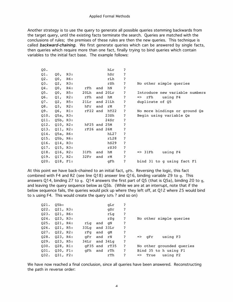
Another strategy is to use the query to generate all possible queries stemming backwards from
the target query, until the existing facts terminate the search. Queries are matched with the
conclusions of rules; the premises of these rules are then the new queries. This technique is
called backward-chaining. We first generate queries which can be answered by single facts,
then queries which require more than one fact, finally trying to bind queries which contain
variables to the initial fact base. The example follows:
Q0. hLr ?Q1. Q0, R3: hSr ?Q2. Q0, R6: rLh ?Q3. Q2, R3: rSh ? No other simple queriesQ4. Q0, R4: rFh and hN ?Q5. Q0, R5: 20Lh and 20Lr ? Introduce new variable numbersQ6. Q1, R2: rFh and hM ? => rFh using F4Q7. Q2, R5: 21Lr and 21Lh ? duplicate of Q5Q8. Q3, R2: hFr and rM ?Q9. Q6, R1: rF22 and hT22 ? No more bindings or ground QsQ10. Q5a, R3: 23Sh ? Begin using variable QsQ11. Q5b, R3: 24Sr ?Q12. Q10, R2: hF25 and 25M ?Q13. Q11, R2: rF26 and 26M ?Q14. Q5a, R6: hL27 ?Q15. Q5b, R6: rL28 ?Q16. Q14, R3: hS29 ?Q17. Q15, R3: rS30 ?Q18. Q16, R2: 31Fh and hM ? => 31Fh using F4Q19. Q17, R2: 32Fr and rM ?Q20. Q18, F1: gFh ? bind 31 to g using fact F1
At this point we have back-chained to an initial fact, gFh. Reversing the logic, this fact
combined with F4 and R2 (see line Q18) answer line Q16, binding variable 29 to g. This
answers Q14, binding 27 to g. Q14 answers the first part of Q5 (that is Q5a), binding 20 to g,
and leaving the query sequence below as Q5b. (While we are at an interrupt, note that if the
below sequence fails, the queries would pick up where they left off, at Q12 where 25 would bind
to h using F4. This would create the query hFh ? and so on)
Q21. Q5b: gLr ?Q22. Q21, R3: gSr ?Q23. Q21, R6: rLg ?Q24. Q23, R3: rSg ? No other simple queriesQ25. Q21, R4: rLg and gN ?Q26. Q21, R5: 33Lg and 33Lr ?Q27. Q22, R2: rFg and gM ?Q28. Q23, R4: gFr and rN ? => gFr using F3Q29. Q23, R5: 34Lr and 34Lg ?Q30. Q28, R1: gF35 and rT35 ? No other grounded queriesQ31. Q30, F1: gFh and rTh ? Bind 35 to h using F1Q32. Q31, F2: rTh ? => True using F2
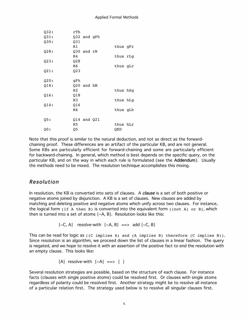
We have now reached a final conclusion, since all queries have been answered. Reconstructing
the path in reverse order:
Applied Formal Methods
5
Q32: rThQ31: Q32 and gFhQ30: Q31
R1 thus gFrQ28: Q30 and rN
R4 thus rLgQ23: Q28
R6 thus gLrQ21: Q23
Q20: gFhQ18: Q20 and hM
R2 thus hSgQ16: Q18
R3 thus hLgQ14: Q16
R6 thus gLh
Q5: Q14 and Q21R5 thus hLr
Q0: Q5 QED
Note that this proof is similar to the natural deduction, and not as direct as the forward-
chaining proof. These differences are an artifact of the particular KB, and are not general.
Some KBs are particularly efficient for forward-chaining and some are particularly efficient
for backward-chaining. In general, which method is best depends on the specific query, on the
particular KB, and on the way in which each rule is formulated (see the Addendum). Usually
the methods need to be mixed. The resolution technique accomplishes this mixing.
Resolut ion
In resolution, the KB is converted into sets of clauses. A clause is a set of both positive or
negative atoms joined by disjunction. A KB is a set of clauses. New clauses are added by
matching and deleting positive and negative atoms which unify across two clauses. For instance,
the logical form (if A then B) is converted into the equivalent form ((not A) or B), which
then is turned into a set of atoms {~A, B}. Resolution looks like this:
{~C, A} resolve-with {~A, B} ==> add {~C, B}
This can be read for logic as ((C implies A) and (A implies B) therefore (C implies B)).
Since resolution is an algorithm, we proceed down the list of clauses in a linear fashion. The query
is negated, and we hope to resolve it with an assertion of the positive fact to end the resolution with
an empty clause. This looks like:
{A} resolve-with {~A} ==> { }
Several resolution strategies are possible, based on the structure of each clause. For instance
facts (clauses with single positive atoms) could be resolved first. Or clauses with single atoms
regardless of polarity could be resolved first. Another strategy might be to resolve all instance
of a particular relation first. The strategy used below is to resolve all singular clauses first.
Applied Formal Methods
6
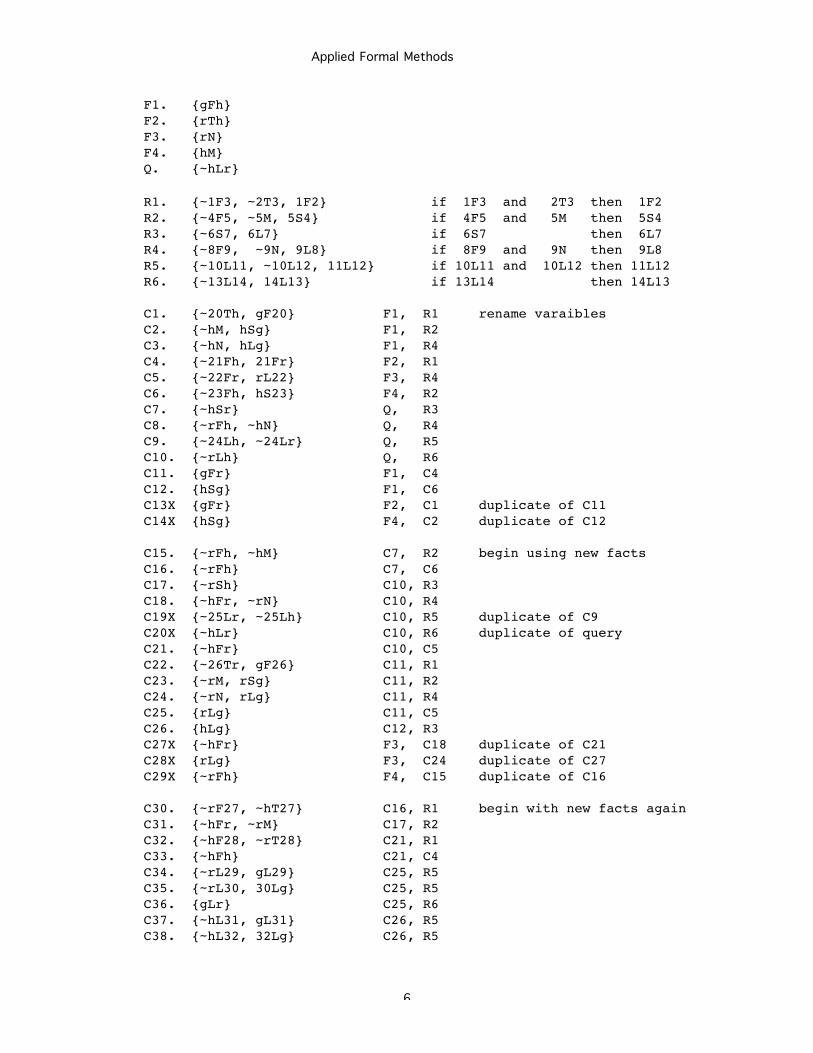
F1. {gFh}F2. {rTh}F3. {rN}F4. {hM}Q. {~hLr}
R1. {~1F3, ~2T3, 1F2} if 1F3 and 2T3 then 1F2R2. {~4F5, ~5M, 5S4} if 4F5 and 5M then 5S4R3. {~6S7, 6L7} if 6S7 then 6L7R4. {~8F9, ~9N, 9L8} if 8F9 and 9N then 9L8R5. {~10L11, ~10L12, 11L12} if 10L11 and 10L12 then 11L12R6. {~13L14, 14L13} if 13L14 then 14L13
C1. {~20Th, gF20} F1, R1 rename varaiblesC2. {~hM, hSg} F1, R2C3. {~hN, hLg} F1, R4C4. {~21Fh, 21Fr} F2, R1C5. {~22Fr, rL22} F3, R4C6. {~23Fh, hS23} F4, R2C7. {~hSr} Q, R3C8. {~rFh, ~hN} Q, R4C9. {~24Lh, ~24Lr} Q, R5C10. {~rLh} Q, R6C11. {gFr} F1, C4C12. {hSg} F1, C6C13X {gFr} F2, C1 duplicate of C11C14X {hSg} F4, C2 duplicate of C12
C15. {~rFh, ~hM} C7, R2 begin using new factsC16. {~rFh} C7, C6C17. {~rSh} C10, R3C18. {~hFr, ~rN} C10, R4C19X {~25Lr, ~25Lh} C10, R5 duplicate of C9C20X {~hLr} C10, R6 duplicate of queryC21. {~hFr} C10, C5C22. {~26Tr, gF26} C11, R1C23. {~rM, rSg} C11, R2C24. {~rN, rLg} C11, R4C25. {rLg} C11, C5C26. {hLg} C12, R3C27X {~hFr} F3, C18 duplicate of C21C28X {rLg} F3, C24 duplicate of C27C29X {~rFh} F4, C15 duplicate of C16
C30. {~rF27, ~hT27} C16, R1 begin with new facts againC31. {~hFr, ~rM} C17, R2C32. {~hF28, ~rT28} C21, R1C33. {~hFh} C21, C4C34. {~rL29, gL29} C25, R5C35. {~rL30, 30Lg} C25, R5C36. {gLr} C25, R6C37. {~hL31, gL31} C26, R5C38. {~hL32, 32Lg} C26, R5
Applied Formal Methods
7
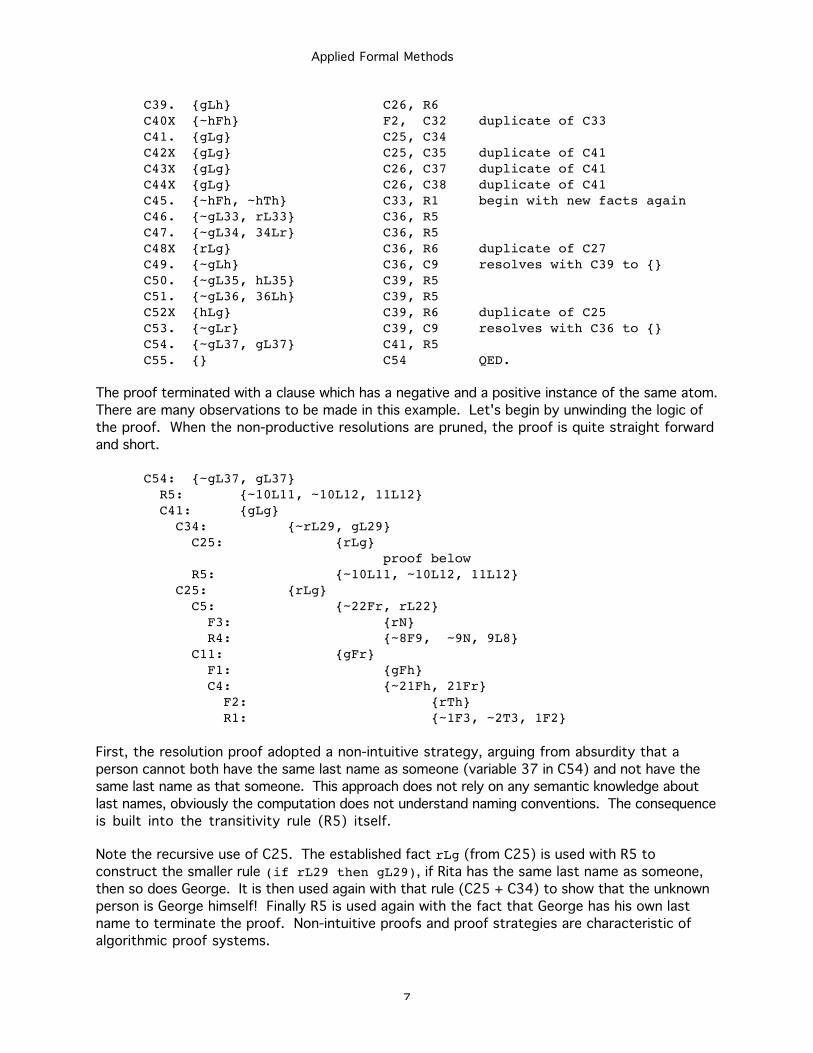
C39. {gLh} C26, R6C40X {~hFh} F2, C32 duplicate of C33C41. {gLg} C25, C34C42X {gLg} C25, C35 duplicate of C41C43X {gLg} C26, C37 duplicate of C41C44X {gLg} C26, C38 duplicate of C41C45. {~hFh, ~hTh} C33, R1 begin with new facts againC46. {~gL33, rL33} C36, R5C47. {~gL34, 34Lr} C36, R5C48X {rLg} C36, R6 duplicate of C27C49. {~gLh} C36, C9 resolves with C39 to {}C50. {~gL35, hL35} C39, R5C51. {~gL36, 36Lh} C39, R5C52X {hLg} C39, R6 duplicate of C25C53. {~gLr} C39, C9 resolves with C36 to {}C54. {~gL37, gL37} C41, R5C55. {} C54 QED.
The proof terminated with a clause which has a negative and a positive instance of the same atom.
There are many observations to be made in this example. Let's begin by unwinding the logic of
the proof. When the non-productive resolutions are pruned, the proof is quite straight forward
and short.
C54: {~gL37, gL37} R5: {~10L11, ~10L12, 11L12} C41: {gLg} C34: {~rL29, gL29} C25: {rLg}
proof below R5: {~10L11, ~10L12, 11L12} C25: {rLg} C5: {~22Fr, rL22} F3: {rN}
R4: {~8F9, ~9N, 9L8} C11: {gFr} F1: {gFh} C4: {~21Fh, 21Fr} F2: {rTh} R1: {~1F3, ~2T3, 1F2}
First, the resolution proof adopted a non-intuitive strategy, arguing from absurdity that a
person cannot both have the same last name as someone (variable 37 in C54) and not have the
same last name as that someone. This approach does not rely on any semantic knowledge about
last names, obviously the computation does not understand naming conventions. The consequence
is built into the transitivity rule (R5) itself.
Note the recursive use of C25. The established fact rLg (from C25) is used with R5 to
construct the smaller rule (if rL29 then gL29), if Rita has the same last name as someone,
then so does George. It is then used again with that rule (C25 + C34) to show that the unknown
person is George himself! Finally R5 is used again with the fact that George has his own last
name to terminate the proof. Non-intuitive proofs and proof strategies are characteristic of
algorithmic proof systems.

Applied Formal Methods
8
The proof would have been substantively different if R6, the commutative rule for last-names
had not been included. In fact, it is not necessary for a proof. In this resolution proof, it is
surprising that R2, R3, R6, and F4 were not used at all, even though from a natural deduction
perspective they appear mandatory.
Note also the many convergent proofs toward the end. Had C54 not occurred, both C49 and C53
would have terminated the proof during the next cycle. Again, multiple paths with high
redundancy are characteristic of algorithmic techniques.
Note also that the distinction between forward and backward chaining is largely lost, since
matching positive facts and negative facts uses the same algorithm without distinction. The
algorithmic proof followed all paths at the same time, taking small steps along each possible
path without regard to conclusions or duplications.
Other control strategies for the resolution would have resulted in different proofs and even
different proof strategies. It may have been more efficient, for example, to resolve the new
facts with the shorter new rules first, before using the original rules, since the original rules
R1 and R5 introduced excess variables.
In resolution, it is possible to resolve rules together, as well as just to follow facts. For
example:
R2. {~4F5, ~5M, 5S4}R3. {~6S7, 6L7} ==> {~20F21, ~21M, 21L20}
This generates a new rule, which is more direct for the purposes of the question that has been
asked. When to do this becomes clear in the following boundary logic approach.
Boundary Logic
Again we transcribe the rules into a new, boundary, notation:
R1: ( ((1F3) (2T3)) ) 1F2 if 1F3 and 2T3 then 1F2R2: ( ((4F5) (5M)) ) 5S4 if 4F5 and 5M then 5S4R3: (6S7) 6L7 if 6S7 then 6L7R4: ( ((8F9) (9N)) ) 9L8 if 8F9 and 9N then 9L8R5: ( ((10L11) (10L12)) ) 11L12 if 10L11 and 10L12 then 11L12R6: (13L14) 14L13 if 13L14 then 14L13
In this notation, some redundant logical structure can be seen at the level of individual rules.
We simplify the rules individually using Involution:
R1: (1F3) (2T3) 1F2R2: (4F5) (5M) 5S4R3: (6S7) 6L7R4: (8F9) (9N) 9L8R5: (10L11) (10L12) 11L12R6: (13L14) 14L13
Applied Formal Methods
9
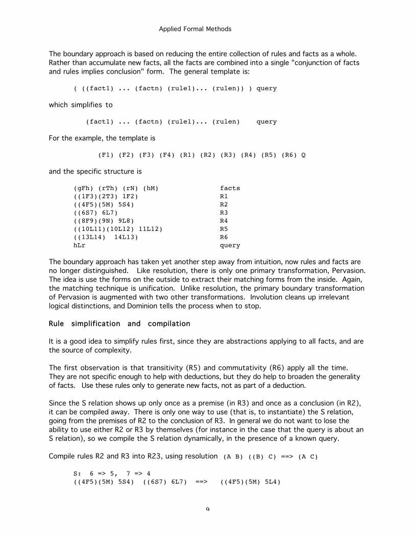
The boundary approach is based on reducing the entire collection of rules and facts as a whole.
Rather than accumulate new facts, all the facts are combined into a single "conjunction of facts
and rules implies conclusion" form. The general template is:
( ((fact1) ... (factn) (rule1)... (rulen)) ) query
which simplifies to
(fact1) ... (factn) (rule1)... (rulen) query
For the example, the template is
(F1) (F2) (F3) (F4) (R1) (R2) (R3) (R4) (R5) (R6) Q
and the specific structure is
(gFh) (rTh) (rN) (hM) facts((1F3)(2T3) 1F2) R1((4F5)(5M) 5S4) R2((6S7) 6L7) R3((8F9)(9N) 9L8) R4((10L11)(10L12) 11L12) R5((13L14) 14L13) R6hLr query
The boundary approach has taken yet another step away from intuition, now rules and facts are
no longer distinguished. Like resolution, there is only one primary transformation, Pervasion.
The idea is use the forms on the outside to extract their matching forms from the inside. Again,
the matching technique is unification. Unlike resolution, the primary boundary transformation
of Pervasion is augmented with two other transformations. Involution cleans up irrelevant
logical distinctions, and Dominion tells the process when to stop.
Rule simplification and compilation
It is a good idea to simplify rules first, since they are abstractions applying to all facts, and are
the source of complexity.
The first observation is that transitivity (R5) and commutativity (R6) apply all the time.
They are not specific enough to help with deductions, but they do help to broaden the generality
of facts. Use these rules only to generate new facts, not as part of a deduction.
Since the S relation shows up only once as a premise (in R3) and once as a conclusion (in R2),
it can be compiled away. There is only one way to use (that is, to instantiate) the S relation,
going from the premises of R2 to the conclusion of R3. In general we do not want to lose the
ability to use either R2 or R3 by themselves (for instance in the case that the query is about an
S relation), so we compile the S relation dynamically, in the presence of a known query.
Compile rules R2 and R3 into R23, using resolution (A B) ((B) C) ==> (A C)
S: 6 => 5, 7 => 4((4F5)(5M) 5S4) ((6S7) 6L7) ==> ((4F5)(5M) 5L4)
Applied Formal Methods
10
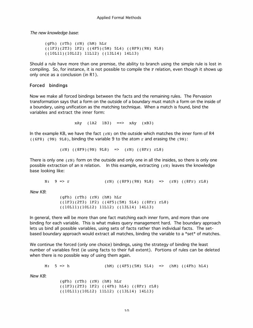
The new knowledge base:
(gFh) (rTh) (rN) (hM) hLr((1F3)(2T3) 1F2) ((4F5)(5M) 5L4) ((8F9)(9N) 9L8)((10L11)(10L12) 11L12) ((13L14) 14L13)
Should a rule have more than one premise, the ability to branch using the simple rule is lost in
compiling. So, for instance, it is not possible to compile the F relation, even though it shows up
only once as a conclusion (in R1).
Forced bindings
Now we make all forced bindings between the facts and the remaining rules. The Pervasion
transformation says that a form on the outside of a boundary must match a form on the inside of
a boundary, using unification as the matching technique. When a match is found, bind the
variables and extract the inner form:
xAy (1A2 1B3) ==> xAy (xB3)
In the example KB, we have the fact (rN) on the outside which matches the inner form of R4
((6F8) (9N) 9L8), binding the variable 9 to the atom r and erasing the (9N):
(rN) ((8F9)(9N) 9L8) => (rN) ((8Fr) rL8)
There is only one (rN) form on the outside and only one in all the insides, so there is only one
possible extraction of an N relation. In this example, extracting (rN) leaves the knowledge
base looking like:
N: 9 => r (rN) ((8F9)(9N) 9L8) => (rN) ((8Fr) rL8)
New KB:(gFh) (rTh) (rN) (hM) hLr((1F3)(2T3) 1F2) ((4F5)(5M) 5L4) ((8Fr) rL8)((10L11)(10L12) 11L12) ((13L14) 14L13)
In general, there will be more than one fact matching each inner form, and more than one
binding for each variable. This is what makes query management hard. The boundary approach
lets us bind all possible variables, using sets of facts rather than individual facts. The set-
based boundary approach would extract all matches, binding the variable to a *set* of matches.
We continue the forced (only one choice) bindings, using the strategy of binding the least
number of variables first (ie using facts to their full extent). Portions of rules can be deleted
when there is no possible way of using them again.
M: 5 => h (hM) ((4F5)(5M) 5L4) => (hM) ((4Fh) hL4)
New KB:(gFh) (rTh) (rN) (hM) hLr((1F3)(2T3) 1F2) ((4Fh) hL4) ((8Fr) rL8)((10L11)(10L12) 11L12) ((13L14) 14L13)
Applied Formal Methods
11
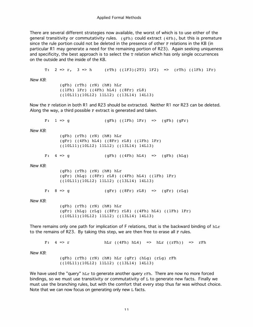
There are several different strategies now available, the worst of which is to use either of the
general transitivity or commutativity rules. (gFh) could extract (4Fh), but this is premature
since the rule portion could not be deleted in the presence of other F relations in the KB (in
particular R1 may generate a need for the remaining portion of R23). Again seeking uniqueness
and specificity, the best approach is to select the T relation which has only single occurrences
on the outside and the inside of the KB.
T: 2 => r, 3 => h (rTh) ((1F3)(2T3) 1F2) => (rTh) ((1Fh) 1Fr)
New KB:(gFh) (rTh) (rN) (hM) hLr((1Fh) 1Fr) ((4Fh) hL4) ((8Fr) rL8)((10L11)(10L12) 11L12) ((13L14) 14L13)
Now the F relation in both R1 and R23 should be extracted. Neither R1 nor R23 can be deleted.
Along the way, a third possible F extract is generated and taken.
F: 1 => g (gFh) ((1Fh) 1Fr) => (gFh) (gFr)
New KB:(gFh) (rTh) (rN) (hM) hLr(gFr) ((4Fh) hL4) ((8Fr) rL8) ((1Fh) 1Fr)((10L11)(10L12) 11L12) ((13L14) 14L13)
F: 4 => g (gFh) ((4Fh) hL4) => (gFh) (hLg)
New KB:(gFh) (rTh) (rN) (hM) hLr(gFr) (hLg) ((8Fr) rL8) ((4Fh) hL4) ((1Fh) 1Fr)((10L11)(10L12) 11L12) ((13L14) 14L13)
F: 8 => g (gFr) ((8Fr) rL8) => (gFr) (rLg)
New KB:(gFh) (rTh) (rN) (hM) hLr(gFr) (hLg) (rLg) ((8Fr) rL8) ((4Fh) hL4) ((1Fh) 1Fr)((10L11)(10L12) 11L12) ((13L14) 14L13)
There remains only one path for implication of F relations, that is the backward binding of hLrto the remains of R23. By taking this step, we are then free to erase all F rules.
F: 4 => r hLr ((4Fh) hL4) => hLr ((rFh)) => rFh
New KB:(gFh) (rTh) (rN) (hM) hLr (gFr) (hLg) (rLg) rFh((10L11)(10L12) 11L12) ((13L14) 14L13)
We have used the "query" hLr to generate another query rFh. There are now no more forced
bindings, so we must use transitivity or commutativity of L to generate new facts. Finally we
must use the branching rules, but with the comfort that every step thus far was without choice.
Note that we can now focus on generating only new L facts.
Applied Formal Methods
12
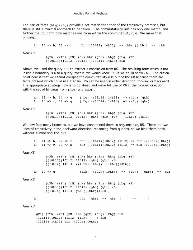
The pair of facts (hLg)(rLg) provide a set match for either of the transitivity premises, but
there is still a minimal approach to be taken. The commutativity rule has only one match, and
further the hLr form only matches one form within the commutativity rule. We make that
binding:
L: 14 => h, 13 => r hLr ((13L14) 14L13) => hLr ((rLh)) => rLh
New KB:(gFh) (rTh) (rN) (hM) hLr (gFr) (hLg) (rLg) rFh((10L11)(10L12) 11L12) ((13L14) 14L13) rLh
Above, we used the query hLr to extract a conclusion from R6. The resulting form which is not
inside a boundary is also a query; that is, we would know hLr if we could show rLh. The critical
point here is that we cannot collapse the commutativity rule out of the KB because there are
facts present which could use it again. R6 can be used in either direction, forward or backward.
The appropriate strategy now is to go ahead and make full use of R6 in the forward direction,
with the set of bindings from (hLg) and (rLg):
L: 13 => h, 14 => g (hLg) ((13L14) 14L13) => (hLg) (gLh)L: 13 => r, 14 => g (rLg) ((13L14) 14L13) => (rLg) (gLr)
New KB:(gFh) (rTh) (rN) (hM) hLr (gFr) (hLg) (rLg) rFh((10L11)(10L12) 11L12) (gLh) (gLr) rLh ((13L14) 14L13)
We now face many branches, but we have constrained them to only one rule, R5. There are two
uses of transitivity in the backward direction, reasoning from queries, so we bind them both,
without eliminating the rule.
L: 11 => h, 12 => r hLr ((10L11)(10L12) 11L12) => hLr ((10Lh)(10Lr))L: 11 => r, 12 => h rLh ((10L11)(10L12) 11L12) => rLh ((10Lr)(10Lh))
New KB:(gFh) (rTh) (rN) (hM) hLr (gFr) (hLg) (rLg) rFh((10L11)(10L12) 11L12) (gLh) (gLr) rLh((13L14) 14L13) ((10Lh)(10Lr)) ((10Lr)(10Lh))
L: 10 => g (gLh) ((10Lh)(10Lr)) => (gLh) ((gLr)) => gLr
New KB:(gFh) (rTh) (rN) (hM) hLr (gFr) (hLg) (rLg) rFh ((10L11)(10L12) 11L12) (gLh) (gLr) rLh((13L14) 14L13) gLr ((10Lr)(10Lh))
L: gLr (gLr) => gLr ( ) => ( )
New KB:
(gFh) (rTh) (rN) (hM) hLr (gFr) (hLg) (rLg) rFh((10L11)(10L12) 11L12) (gLh) ( ) rLh((13L14) 14L13) gLr ((10Lr)(10Lh))
Applied Formal Methods
13
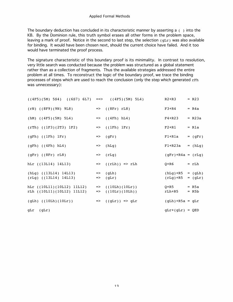
The boundary deduction has concluded in its characteristic manner by asserting a ( ) into the
KB. By the Dominion rule, this truth symbol erases all other forms in the problem space,
leaving a mark of proof. Notice in the second to last step, the selection (gLr) was also available
for binding. It would have been chosen next, should the current choice have failed. And it too
would have terminated the proof process.
The signature characteristic of this boundary proof is its minimality. In contrast to resolution,
very little search was conducted because the problem was structured as a global statement
rather than as a collection of fragments. Thus the available strategies addressed the entire
problem at all times. To reconstruct the logic of the boundary proof, we trace the binding
processes of steps which are used to reach the conclusion (only the step which generated rFhwas unnecessary):
((4F5)(5M) 5S4) ((6S7) 6L7) ==> ((4F5)(5M) 5L4) R2+R3 = R23
(rN) ((8F9)(9N) 9L8) => ((8Fr) rL8) F3+R4 = R4a
(hM) ((4F5)(5M) 5L4) => ((4Fh) hL4) F4+R23 = R23a
(rTh) ((1F3)(2T3) 1F2) => ((1Fh) 1Fr) F2+R1 = R1a
(gFh) ((1Fh) 1Fr) => (gFr) F1+R1a = (gFr)
(gFh) ((4Fh) hL4) => (hLg) F1+R23a = (hLg)
(gFr) ((8Fr) rL8) => (rLg) (gFr)+R4a = (rLg)
hLr ((13L14) 14L13) => ((rLh)) => rLh Q+R6 = rLh
(hLg) ((13L14) 14L13) => (gLh) (hLg)+R5 = (gLh)(rLg) ((13L14) 14L13) => (gLr) (rLg)+R5 = (gLr)
hLr ((10L11)(10L12) 11L12) => ((10Lh)(10Lr)) Q+R5 = R5arLh ((10L11)(10L12) 11L12) => ((10Lr)(10Lh)) rLh+R5 = R5b
(gLh) ((10Lh)(10Lr)) => ((gLr)) => gLr (gLh)+R5a = gLr
gLr (gLr) gLr+(gLr) = QED
Applied Formal Methods
14
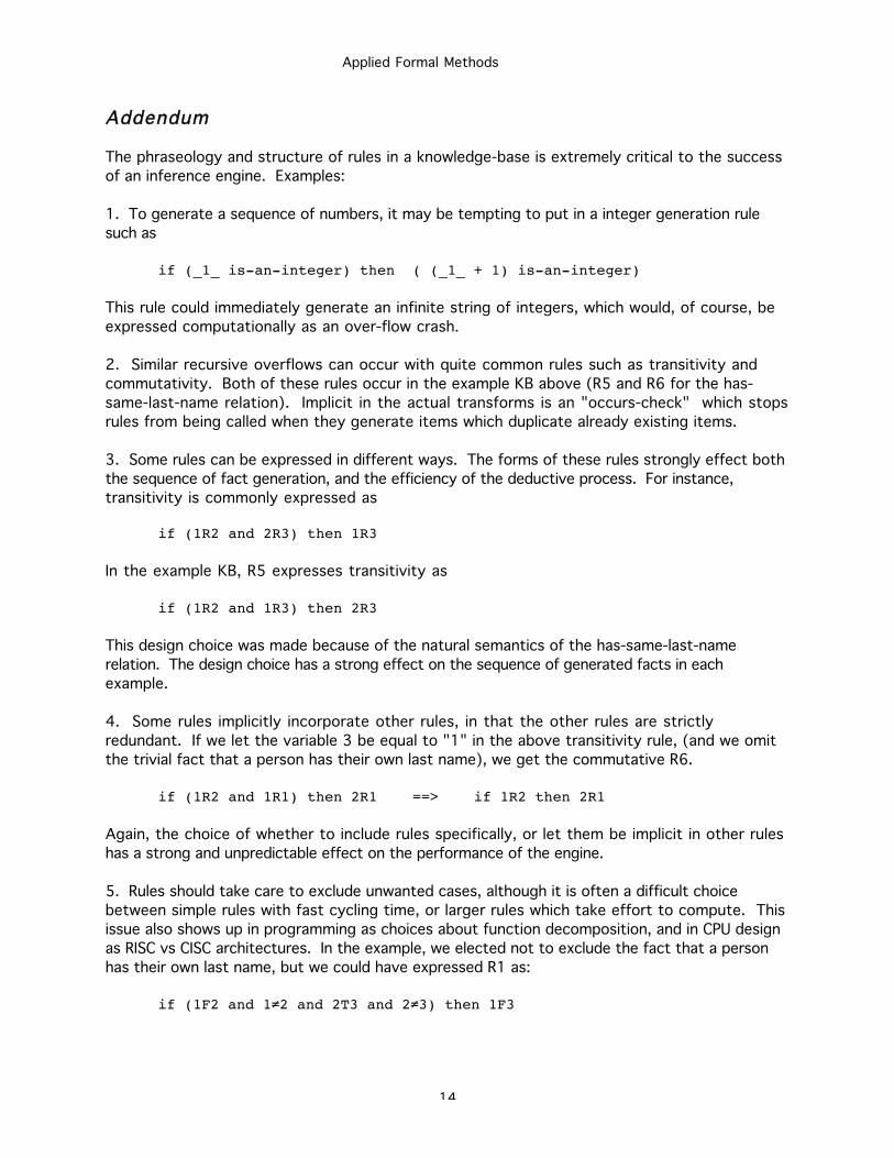
Addendum
The phraseology and structure of rules in a knowledge-base is extremely critical to the success
of an inference engine. Examples:
1. To generate a sequence of numbers, it may be tempting to put in a integer generation rule
such as
if (_1_ is-an-integer) then ( (_1_ + 1) is-an-integer)
This rule could immediately generate an infinite string of integers, which would, of course, be
expressed computationally as an over-flow crash.
2. Similar recursive overflows can occur with quite common rules such as transitivity and
commutativity. Both of these rules occur in the example KB above (R5 and R6 for the has-
same-last-name relation). Implicit in the actual transforms is an "occurs-check" which stops
rules from being called when they generate items which duplicate already existing items.
3. Some rules can be expressed in different ways. The forms of these rules strongly effect both
the sequence of fact generation, and the efficiency of the deductive process. For instance,
transitivity is commonly expressed as
if (1R2 and 2R3) then 1R3
In the example KB, R5 expresses transitivity as
if (1R2 and 1R3) then 2R3
This design choice was made because of the natural semantics of the has-same-last-name
relation. The design choice has a strong effect on the sequence of generated facts in each
example.
4. Some rules implicitly incorporate other rules, in that the other rules are strictly
redundant. If we let the variable 3 be equal to "1" in the above transitivity rule, (and we omit
the trivial fact that a person has their own last name), we get the commutative R6.
if (1R2 and 1R1) then 2R1 ==> if 1R2 then 2R1
Again, the choice of whether to include rules specifically, or let them be implicit in other rules
has a strong and unpredictable effect on the performance of the engine.
5. Rules should take care to exclude unwanted cases, although it is often a difficult choice
between simple rules with fast cycling time, or larger rules which take effort to compute. This
issue also shows up in programming as choices about function decomposition, and in CPU design
as RISC vs CISC architectures. In the example, we elected not to exclude the fact that a person
has their own last name, but we could have expressed R1 as:
if (1F2 and 1 2 and 2T3 and 2 3) then 1F3
Applied Formal Methods
15
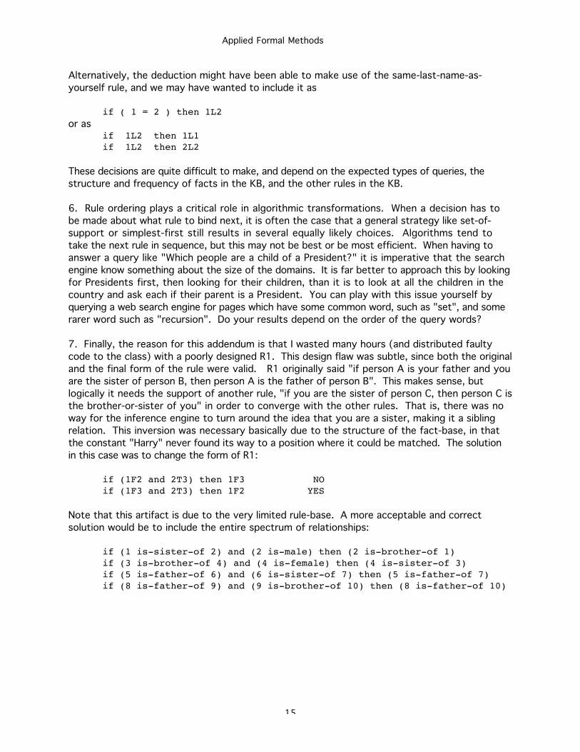
Alternatively, the deduction might have been able to make use of the same-last-name-as-
yourself rule, and we may have wanted to include it as
if ( 1 = 2 ) then 1L2or as
if 1L2 then 1L1if 1L2 then 2L2
These decisions are quite difficult to make, and depend on the expected types of queries, the
structure and frequency of facts in the KB, and the other rules in the KB.
6. Rule ordering plays a critical role in algorithmic transformations. When a decision has to
be made about what rule to bind next, it is often the case that a general strategy like set-of-
support or simplest-first still results in several equally likely choices. Algorithms tend to
take the next rule in sequence, but this may not be best or be most efficient. When having to
answer a query like "Which people are a child of a President?" it is imperative that the search
engine know something about the size of the domains. It is far better to approach this by looking
for Presidents first, then looking for their children, than it is to look at all the children in the
country and ask each if their parent is a President. You can play with this issue yourself by
querying a web search engine for pages which have some common word, such as "set", and some
rarer word such as "recursion". Do your results depend on the order of the query words?
7. Finally, the reason for this addendum is that I wasted many hours (and distributed faulty
code to the class) with a poorly designed R1. This design flaw was subtle, since both the original
and the final form of the rule were valid. R1 originally said "if person A is your father and you
are the sister of person B, then person A is the father of person B". This makes sense, but
logically it needs the support of another rule, "if you are the sister of person C, then person C is
the brother-or-sister of you" in order to converge with the other rules. That is, there was no
way for the inference engine to turn around the idea that you are a sister, making it a sibling
relation. This inversion was necessary basically due to the structure of the fact-base, in that
the constant "Harry" never found its way to a position where it could be matched. The solution
in this case was to change the form of R1:
if (1F2 and 2T3) then 1F3 NOif (1F3 and 2T3) then 1F2 YES
Note that this artifact is due to the very limited rule-base. A more acceptable and correct
solution would be to include the entire spectrum of relationships:
if (1 is-sister-of 2) and (2 is-male) then (2 is-brother-of 1)if (3 is-brother-of 4) and (4 is-female) then (4 is-sister-of 3)if (5 is-father-of 6) and (6 is-sister-of 7) then (5 is-father-of 7)if (8 is-father-of 9) and (9 is-brother-of 10) then (8 is-father-of 10)
Applied Formal Methods
1
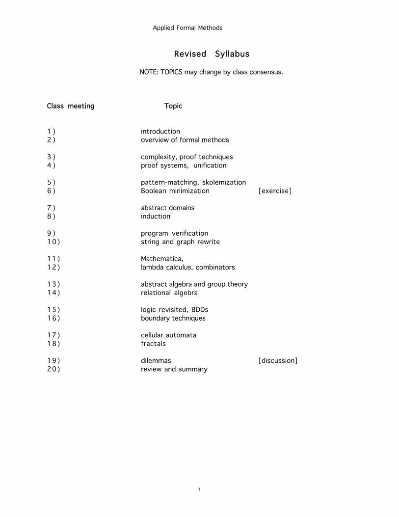
Revised Syllabus
NOTE: TOPICS may change by class consensus.
Class meeting Topic
1 ) introduction
2 ) overview of formal methods
3 ) complexity, proof techniques
4 ) proof systems, unification
5 ) pattern-matching, skolemization
6 ) Boolean minimization [exercise]
7 ) abstract domains
8 ) induction
9 ) program verification
10) string and graph rewrite
11) Mathematica,
12) lambda calculus, combinators
13) abstract algebra and group theory
14) relational algebra
15) logic revisited, BDDs
16) boundary techniques
17) cellular automata
18) fractals
19) dilemmas [discussion]
20) review and summary
Applied Formal Methods
1
Class Handouts; Exploration Project
The following readings have been selected as relatively clear and concise summary articles for
specific topics. There is no textbook for the class. Of course, all students are expected to access
the Internet to find additional information for any topic.
There will be a lot of reading material, and some of it will be fairly technical. Students are
expected to read all of the class handouts before class. Students should scan each of the articles,
read and study parts which are of interest, and ask questions in class about unclear areas.
In-Depth Exploration Project
Each student will explore in depth one particular topic, and report to the class their
experiences while learning about that topic. The presentation should be a chronicle of
experiences while exploring the topic, including high and low points, confusions, learnings,
false paths, discovered treasures, treacherous territories, and an overall evaluation of the
utility of the topic.
Efforts solely to impress the instructor or to generate a pretty report should be avoided.
Efforts to clarify the ideas of the topic are encouraged, however, students will not be
responsible for teaching the content of a topic to the class. Students who locate particularly good
or interesting articles on a topic are encouraged to add these articles (or websites) to the class
reading list.
Handouts
WEEK 1:
ClassNotes 1: Course Information, Variety of Formal Methods, References, Web Pointers
ClassNotes 2: Modeling with Logic, Proof Techniques, Quantification, Complexity,
Boundary Techniques
ClassNotes 3: Proof Techniques Extended Example
Stuart Shapiro, Ed. (1987) Encyclopedia of Artificial Intelligence, Wiley
Articles on Pattern Matching, Predicate Logic, and Theorem Proving
John Lucas (1990) Introduction to Abstract Mathematics Second EditionCh 2 Mathematical Proof
David Gries (1981) The Science of Programming, Springer-Verlag
Part 0: Why Use Logic? Why Prove Programs Correct?
Randy Katz (1994) Contemporary Logic Design, Cummings
Figures from front cover
Applied Formal Methods
2
WEEK 2:
ClassNotes 4: Syllabus
ClassNotes 5: Handouts, Exploration Project
ClassNotes 6: Evolution of Tools
ClassNotes 7: Pattern Encoding
Jonathan Bowen (1996) Ten Commandments of Formal Methods
Oxford University Computing Lab Technical Memo
see http://www.comlab.ox.ac.uk/oucl/people/jonathan.bowen.html
William Bricken (1987) Analyzing Errors in Elementary Mathematics, Stanford University
Appendix I: The Canons of Formal Symbol Systems
Matt Kaufmann (1987) Skolemization explained simply,
Computational Logic Inc Internal Note #27
Peter Burke (1987) Naming and Knowledge, UCLA Computer Science Dept.
WEEK 3:
ClassNotes 8: Combinational Minimization Exercise
Bertram Meyer (1985) On Formalism in Specifications,
in IEEE Software 1/85
Thomas L. Floyd (1998) Digital Fundamentals Fifth Edition, Prentice-Hall
4.11 Digital System Application, The 7-Segment Display
Giovanni DeMicheli (1994) Synthesis and Optimization of Digital Circuits, McGraw-Hill
Ch 8 Multiple-level Combinational Logic Optimization
John Oldfield and Richard Korf (1995) Field-Programmable Gate Arrays, Wiley
Ch 4. Design Process Flows and Software Tools
WEEK 4:
ClassNotes 9: Domain Theories, Strings, Trees, Sets, Rational Numbers
ClassNotes 10: Induction and Recursion
Jean-Pierre Banatre and Daniel LeMetayer (1993) Programming by Multiset Transformation,
in CACM V36(1), 1/93
Applied Formal Methods
3
WEEK 5:
ClassNotes 10: Program Verification
ClassNotes 11: Mathematica
Stephen Wolfram (1996) The Mathematica Book Third Edition, Wolfram Media
A Tour of Mathematica, 2.3 Patterns,
Mathematica as a Programming Language (from Second Edition)
WEEK 6:
William Bricken (1994) Pattern-Matching and Function Theory,
Oz Incorporated Technical Memo
John Backus (1977) Turing Award Lecture: Can Programming be Liberated from the
VonNeumann Style? A Functional Style and Its Algebra of Programs
J. Barkley Rosser (1984) Highlights of the History of Lambda-Calculus,
in Annals of the History of Computing V6(4) 10/84.
Guy Cousineau (1990) The Categorical Abstract Machine,
in Gerard Huet (Ed) Logical Foundations of Functional Programming, Addison-Wesley
WEEK 7:
ClassNotes 12: Relational Algebra
Peter Gray (1984) Logic, Algebra and Databases, Ellis Horwood
Ch 6 The Relational Model
J. Hoffman (1997) Introduction to Structured Query Language
http://w3.one.net/~jhoffman/sqltut.htm
WEEK 8:
William Bricken (1983) Fractal Dimensions, Atari Systems Research Internal Memo
Richard Feynman (1996) Feynman Lectures on Computation, Addison-Wesley
2.3, 5.4, 5.5 On Reversible Computation
WEEKS 9 and 10:
ClassNotes 13: Summary, Philosophical Dilemmas
Applied Formal Methods
1
An Evolution of Mathematical Tools
From Conceptualization to Formalization
Here's what we do when we build a formal model (or do a computation):
0. Identify a collection of objects/events in the real world. This is the semantic mapping, how
math is linked with reality. The objects/events must have these properties:
unique, not confused with different objects/events
stable and permanent, not in flux or changing too rapidly to identify
discrete, not lacking well defined borders
comprehendible, not confusing or too ambiguous
relevant, not outside of what we consider to be the objects in question
permitted, not in violation of tacit understandings about how things are
1. Use unique labels to identify each of the things in the semantic mapping. The value of a label
is the thing it identifies.
2. Limit our interest in the types of things in the real world to an abstract mathematical
property, such as Truth or Count or Membership.
3. Use different labels to name different abstract things:
labels for things object labelslabels for an entire set of things property labelslabels for an arbitrary thing in the set variable labelslabels to name properties of things indirectly function labelslabels to name combinations of things relation labels
4. Follow the rules of symbol transformation in manipulating the labels as if they were the
things. However, the labels do not have to share any of the real world properties of the physical
things.
In summary, we convert from physical to virtual, ignore the physical aspects of reality,
manipulate the virtual (or digital) aspects using the rules of virtuality, and then return to
physical reality with new knowledge. The rules of virtuality are listed in the handout TheCanons of Formal Symbol Systems.
Virtuality has become so prevalent in the current Information Age that much of what we do is
never part of physical reality in the first place. Computer Science, for example, is a discipline
in which the only connection to physical reality is silicon hardware. Study of the physicality of
hardware is a different discipline, Electrical Engineering.
Computational hardware is engineered (constructed) to behave as if it were a mathematical
system called Timed Boolean Logic. “Timed” simply means that some parts of the physical
hardware are used more than once to do the Boolean logic task for which they were constructed.
Applied Formal Methods
2
Formal Simplicity
The simplest interesting formal domain is PPropositional Calculus, also known as Boolean
Logic, and also known as BBoolean Algebra.
In Boolean algebra, the labels for real world objects are sentences in human language which can
be evaluated as either True or False. These sentences are composed of atoms (propositions) and
logical connectives. The atoms are labels for things which exist and are in some way actual, or
real, or True. The logical connectives are those parts of language which do not refer to
something in physical reality.
More generally, Boolean algebra includes all of decision theory, which phrases a problem space
as a sequence of binary decisions. (Note that more complex decisions can usually be phrased as a
collection of binary decisions.)
The truth of a sentence, the direction of a decision, and the voltage in a digital circuit wire are
all binary properties. Every object label in a Boolean problem has the binary property, either
0 or 1, and that is the only property of interest. Logic is the set of rules which maintains the
invariance of the value of binary properties.
Labeling Reality
Let {a, b, c, ...} be simple Boolean variables identifying a set of decision events, each either 0
or 1.
The ways which we combine Boolean variables have been part of our language from antiquity.
They are the familiar operators: {not, or, and, if, equal, if-then-else}. Combinations of
Boolean operators and Boolean variables are called sentences or expressions.
Let {A, B, C, ...} be names of Boolean expressions.
Valid Boolean expressions are defined recursively,
a simple variables are expressions
not A negated expressions are expressions
A or B expressions joined by disjunction are expressions
Since all other Boolean operators can be expressed in terms of nnot and oor, they are all included
in the above definition. This definition means that Boolean expressions are composable and
decomposable; the recursive rules provide Constructors and Accessors.
Symbolic Complexity
The truth table (or Boolean property table) of a Boolean operator specifies how that operator
combines the Boolean properties, or the values, joined by the operator. But here things start to
get complex. Mainly, we can form a huge variety of expressions, and to find the Boolean value of
any expression, we must examine a table with a size exponential in the number of variables
Applied Formal Methods
3
(2^n entries). So a logic circuit with 200 input variables requires an impractical 2^200 rows
in the truth table.
So all decision problems which require a large number of decisions become intractably
inconvenient to examine in the whole. Boolean algebra provides transformation rules which
hold for all expressions, regardless of which Boolean value an expression has. For example,
not (not A) = A
is valid regardless of the expression A.
Axioms and Theorems
Transformation rules can be decomposed into axioms and theorems. The axioms are a minimal
set of rules which preserve the Boolean property and serve as a basis for all other possible
theorems. All the axioms of an axiomatic formal system can be compressed into one single,
usually complex axiom. For Boolean logic, the simplest single axiom which supports all other
Boolean transformations is the Kauffman/Flagg formalization:
(A or B) and (A or (not B)) = A
Similarly, the Resolution rule is a single rule which supports all Boolean transformation. The
many rules of Natural Deduction provide another, more complex set of axioms. One
particularly simple set of supporting axioms (Bricken’s formalization of Boundary Logic) is
the following:
A or True = True
not (not A) = A
A or (not (A or B)) = A or (not B)
This set is particularly useful for pattern-matching and automated deduction, since the patterns
to be matched are relatively simple, and the right-hand-side of each equation is simpler than
the left-hand-side solely through erasing something from the right-hand-side.
P roo f
Boolean algebra axioms and theorems (valid transformations) provide a way to explore decision
spaces without making the actual decisions. This is called logical or algebraic proof. However,
the situation remains complex because now we must select which theorem to apply and where to
apply it. Although the search space is more abstract, it is still intractable and inconvenient.
Although Boolean algebra abstracts the physical properties of decisions, it is still a real worldproblem to use Boolean algebra efficiently.
Predicate Calculus
The next extension to mathematical technique is to permit more complex types of objects.
Instead of being restricted to atoms with no internal complexity, predicate logic lets us form
complex objects in two ways:
Applied Formal Methods
4
1. Quantification:
Property labels were introduced at the very beginning in order to identify a set of things we
wish to talk about. Without them, we could not group any things together, we could only talk
about specific particular things. (This is the difference between Arithmetic and Algebra.)
Quantification lets us address sets or collections of things directly within a logical expression.
The fforall quantifier permits transformation of property labels (entire sets) rather than only
individual members of the set. The eexists quantifier allows us to refer to the existence of at
least one object in a set, a generic object, without saying which particular object we are talking
about. The generic object is an arbitrary object; we choose one object from the set of interest,
but we do not say exactly which object it is. Thus, the generic object can stand in place of any
particular object in a collection.
2a. Relations:
Instead of non-decomposable atoms having a Boolean property, we permit arbitrary
compositions of atoms to have that property. The arbitrary compositions, or relations, are
specified by a table of associations. If the association is in the table, then the relation between
two (or more) simple objects is True, otherwise it is False. Only simple objects or atoms can
be in relationship to each other. Expressions cannot be in a relation, but a relation (such as
aRb), is an expression and can be combined with other expressions by Boolean operators.
2b. Functions:
Technically functions are a structured subset of relations, since FF(a)=b can be expressed as
aFb=True. Functions let us name objects indirectly by naming other objects and the function
which tells us how to get to the object in question. For instance, the function aadd1 moves us
from one integer to the next.
The two extensions are sufficient to characterize all of standard mathematics, and therefore all
of computation.
Other Formal Systems
The art of mathematical modeling is to find properties of real world objects which are both
understood mathematically (i.e. formal) and useful for physical description. Predicate calculus
provides the framework for formally defining arbitrary properties, but without special
computational techniques, each structure becomes difficult to use for computation. Other
formal systems provide specialized techniques for speeding up particular types of computation.
Induction/Recursion: This fundamental technique lets us work with a general case of a set of
expressions, so long as the entire set is in some way structured by an ordering relation. We can
then analyze entire classes of expressions by looking at only the base case and the general
recursive case. This then provides a programming style.
Applied Formal Methods
5
Relational Calculus: The techniques of computing with only relations have been developed by
the relational database community. The query language SQL exemplifies this approach.
Lambda Calculus: Likewise, the techniques of computing using only functions have been
developed primarily as programming languages by the functional programming community.
Combinators: The combinator calculus is an elaboration of lambda calculus which turns
functional operations into string operations. The specific abstraction technique removes all
variable labels.
String Rewrite Theory: When expressions are represented by strings of tokens, the rules
of transformation can be formulated as changes in the strings, using matching and substitution
for effecting changes. This is the primary technique of mathematical manipulation and of
theorem proving.
Graph Theory: Almost all data structures can be expressed using graphs. A graph rewrite
theory supports valid graph transformations. As well, the graph data structure provides
information about the problem itself, such as the shortest path (fewest number of
transformations) to get from one expression to an equivalent one. This extremely general
technique is underdeveloped solely because graphs are two dimensional structures, while
language has developed using one dimensional strings.
Probability Theory: When the property of interest is a composite of the individual
properties of a sample of objects, that property is a probability, and the rules for manipulating
this statistical object are expressed as probability theory.
Cellular Automata: This is an exotic formal system based on a regular array of autonomous
cells acting on their local neighborhoods. These models have limited but growing applicability.
Fractals: This technique is based on recursive functions usually expressed on a set of two or
higher dimensional objects. Again, fractals are new since they apply to spatial rather than
linear structures.
Boundary Mathematics: This is a general technique which converts all mathematical
string-based operations (logic, sets, numbers, and equations) into spatial operations. The zero
concept is the Void, that is, no representation at all. As a consequence, Boundary Mathematics is
far more efficient in both representation and in transformation than all other mathematical
formalisms. As a spatial technique, it suffers from both unfamiliarity and from the cultural
bias of expressing mathematical operations in string languages.
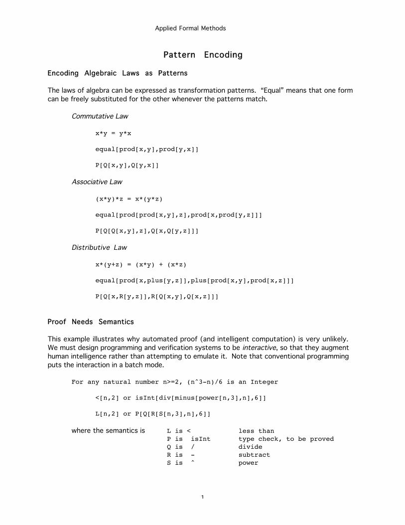
Applied Formal Methods
1
Pattern Encoding
Encoding Algebraic Laws as Patterns
The laws of algebra can be expressed as transformation patterns. “Equal” means that one form
can be freely substituted for the other whenever the patterns match.
Commutative Law
x*y = y*x
equal[prod[x,y],prod[y,x]]
P[Q[x,y],Q[y,x]]
Associative Law
(x*y)*z = x*(y*z)
equal[prod[prod[x,y],z],prod[x,prod[y,z]]]
P[Q[Q[x,y],z],Q[x,Q[y,z]]]
Distributive Law
x*(y+z) = (x*y) + (x*z)
equal[prod[x,plus[y,z]],plus[prod[x,y],prod[x,z]]]
P[Q[x,R[y,z]],R[Q[x,y],Q[x,z]]]
Proof Needs Semantics
This example illustrates why automated proof (and intelligent computation) is very unlikely.
We must design programming and verification systems to be interactive, so that they augment
human intelligence rather than attempting to emulate it. Note that conventional programming
puts the interaction in a batch mode.
For any natural number n>=2, (n^3-n)/6 is an Integer
<[n,2] or isInt[div[minus[power[n,3],n],6]]
L[n,2] or P[Q[R[S[n,3],n],6]]
where the semantics is L is < less thanP is isInt type check, to be provedQ is / divideR is - subtractS is ^ power
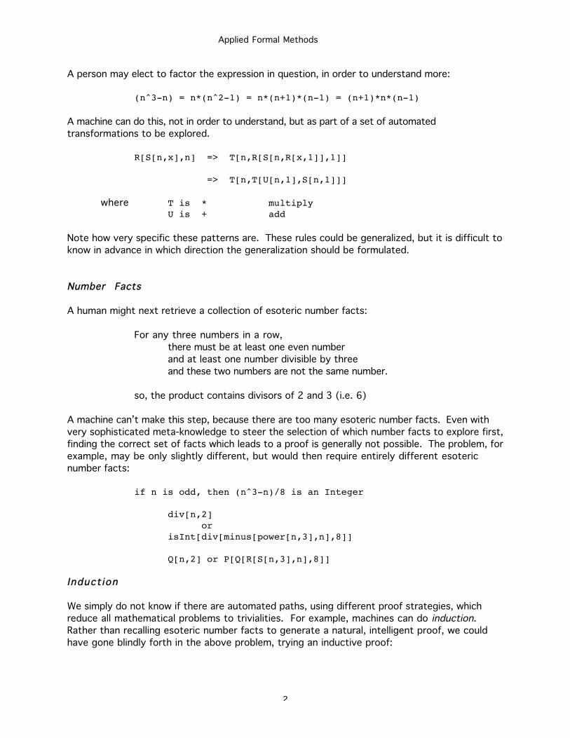
Applied Formal Methods
2
A person may elect to factor the expression in question, in order to understand more:
(n^3-n) = n*(n^2-1) = n*(n+1)*(n-1) = (n+1)*n*(n-1)
A machine can do this, not in order to understand, but as part of a set of automated
transformations to be explored.
R[S[n,x],n] => T[n,R[S[n,R[x,1]],1]]
=> T[n,T[U[n,1],S[n,1]]]
where T is * multiplyU is + add
Note how very specific these patterns are. These rules could be generalized, but it is difficult to
know in advance in which direction the generalization should be formulated.
Number Facts
A human might next retrieve a collection of esoteric number facts:
For any three numbers in a row,
there must be at least one even number
and at least one number divisible by three
and these two numbers are not the same number.
so, the product contains divisors of 2 and 3 (i.e. 6)
A machine can’t make this step, because there are too many esoteric number facts. Even with
very sophisticated meta-knowledge to steer the selection of which number facts to explore first,
finding the correct set of facts which leads to a proof is generally not possible. The problem, for
example, may be only slightly different, but would then require entirely different esoteric
number facts:
if n is odd, then (n^3-n)/8 is an Integer
div[n,2]or
isInt[div[minus[power[n,3],n],8]]
Q[n,2] or P[Q[R[S[n,3],n],8]]
Induct ion
We simply do not know if there are automated paths, using different proof strategies, which
reduce all mathematical problems to trivialities. For example, machines can do induction.
Rather than recalling esoteric number facts to generate a natural, intelligent proof, we could
have gone blindly forth in the above problem, trying an inductive proof:
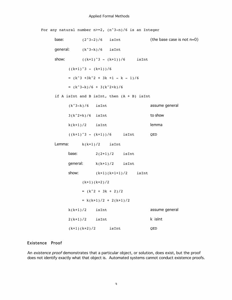
Applied Formal Methods
3
For any natural number n>=2, (n^3-n)/6 is an Integer
base: (2^3-2)/6 isInt (the base case is not n=0)
general: (k^3-k)/6 isInt
show: ((k+1)^3 - (k+1))/6 isInt
((k+1)^3 - (k+1))/6
= (k^3 +3k^2 + 3k +1 - k - 1)/6
= (k^3-k)/6 + 3(k^2+k)/6
if A isInt and B isInt, then (A + B) isInt
(k^3-k)/6 isInt assume general
3(k^2+k)/6 isInt to show
k(k+1)/2 isInt lemma
((k+1)^3 - (k+1))/6 isInt QED
Lemma: k(k+1)/2 isInt
base: 2(2+1)/2 isInt
general: k(k+1)/2 isInt
show: (k+1)(k+1+1)/2 isInt
(k+1)(k+2)/2
= (k^2 + 3k + 2)/2
= k(k+1)/2 + 2(k+1)/2
k(k+1)/2 isInt assume general
2(k+1)/2 isInt k isInt
(k+1)(k+2)/2 isInt QED
Existence Proof
An existence proof demonstrates that a particular object, or solution, does exist, but the proof
does not identify exactly what that object is. Automated systems cannot conduct existence proofs.
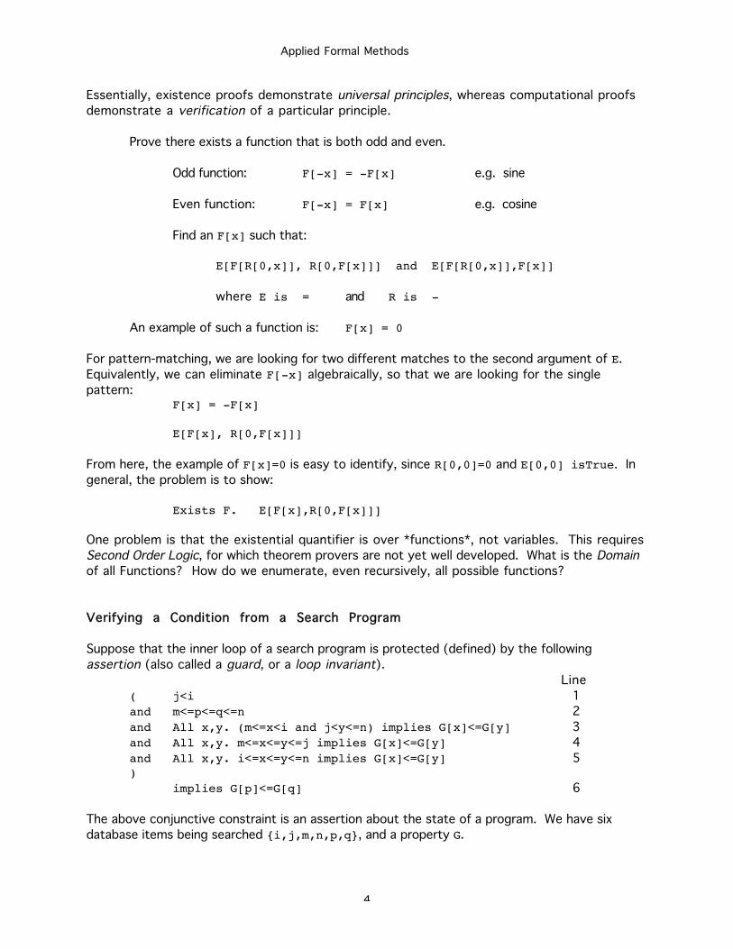
Applied Formal Methods
4
Essentially, existence proofs demonstrate universal principles, whereas computational proofs
demonstrate a verification of a particular principle.
Prove there exists a function that is both odd and even.
Odd function: F[-x] = -F[x] e.g. sine
Even function: F[-x] = F[x] e.g. cosine
Find an F[x] such that:
E[F[R[0,x]], R[0,F[x]]] and E[F[R[0,x]],F[x]]
where E is = and R is -
An example of such a function is: F[x] = 0
For pattern-matching, we are looking for two different matches to the second argument of E.
Equivalently, we can eliminate F[-x] algebraically, so that we are looking for the single
pattern:F[x] = -F[x]
E[F[x], R[0,F[x]]]
From here, the example of F[x]=0 is easy to identify, since R[0,0]=0 and E[0,0] isTrue. In
general, the problem is to show:
Exists F. E[F[x],R[0,F[x]]]
One problem is that the existential quantifier is over *functions*, not variables. This requires
Second Order Logic, for which theorem provers are not yet well developed. What is the Domainof all Functions? How do we enumerate, even recursively, all possible functions?
Verifying a Condition from a Search Program
Suppose that the inner loop of a search program is protected (defined) by the following
assertion (also called a guard, or a loop invariant).Line
( j<i 1
and m<=p<=q<=n 2
and All x,y. (m<=x<i and j<y<=n) implies G[x]<=G[y] 3
and All x,y. m<=x<=y<=j implies G[x]<=G[y] 4
and All x,y. i<=x<=y<=n implies G[x]<=G[y] 5)
implies G[p]<=G[q] 6
The above conjunctive constraint is an assertion about the state of a program. We have six
database items being searched {i,j,m,n,p,q}, and a property G.
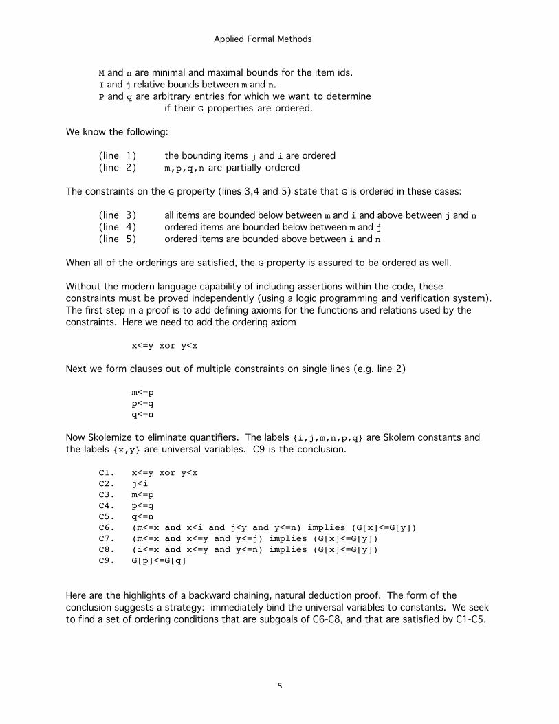
Applied Formal Methods
5
M and n are minimal and maximal bounds for the item ids.
I and j relative bounds between m and n.
P and q are arbitrary entries for which we want to determine
if their G properties are ordered.
We know the following:
(line 1) the bounding items j and i are ordered
(line 2) m,p,q,n are partially ordered
The constraints on the G property (lines 3,4 and 5) state that G is ordered in these cases:
(line 3) all items are bounded below between m and i and above between j and n(line 4) ordered items are bounded below between m and j(line 5) ordered items are bounded above between i and n
When all of the orderings are satisfied, the G property is assured to be ordered as well.
Without the modern language capability of including assertions within the code, these
constraints must be proved independently (using a logic programming and verification system).
The first step in a proof is to add defining axioms for the functions and relations used by the
constraints. Here we need to add the ordering axiom
x<=y xor y<x
Next we form clauses out of multiple constraints on single lines (e.g. line 2)
m<=pp<=qq<=n
Now Skolemize to eliminate quantifiers. The labels {i,j,m,n,p,q} are Skolem constants and
the labels {x,y} are universal variables. C9 is the conclusion.
C1. x<=y xor y<xC2. j<iC3. m<=pC4. p<=qC5. q<=nC6. (m<=x and x<i and j<y and y<=n) implies (G[x]<=G[y])C7. (m<=x and x<=y and y<=j) implies (G[x]<=G[y])C8. (i<=x and x<=y and y<=n) implies (G[x]<=G[y])C9. G[p]<=G[q]
Here are the highlights of a backward chaining, natural deduction proof. The form of the
conclusion suggests a strategy: immediately bind the universal variables to constants. We seek
to find a set of ordering conditions that are subgoals of C6-C8, and that are satisfied by C1-C5.
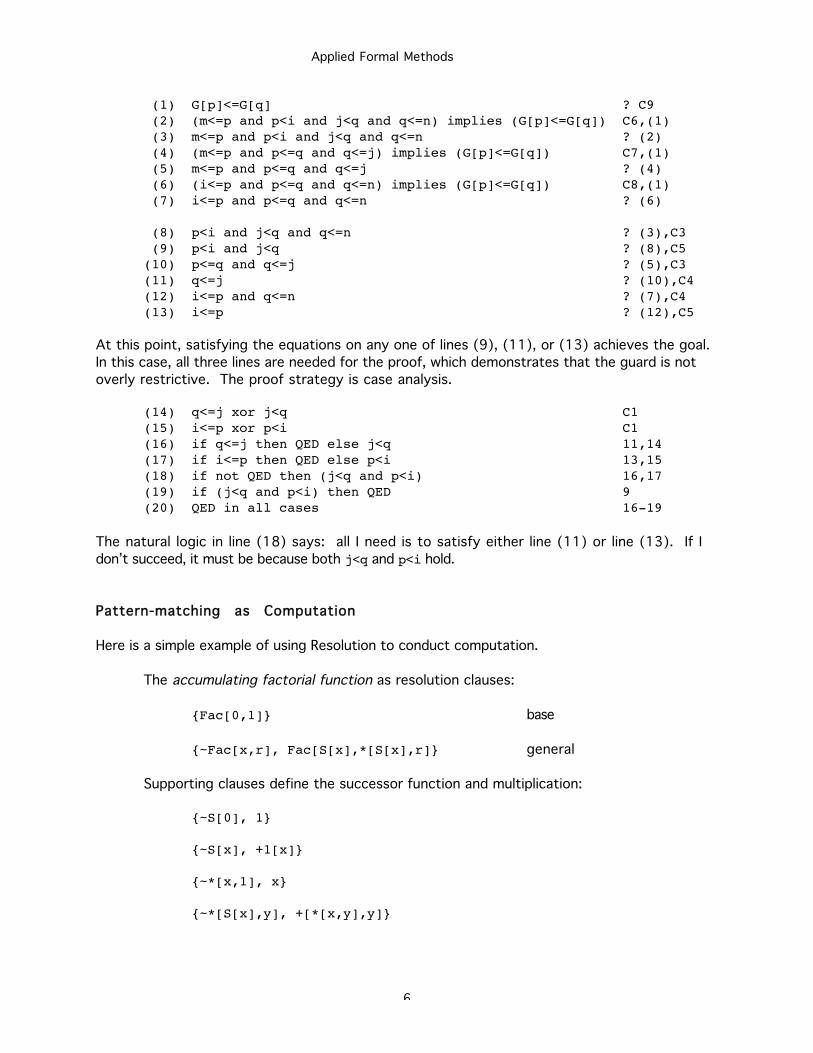
Applied Formal Methods
6
(1) G[p]<=G[q] ? C9 (2) (m<=p and p<i and j<q and q<=n) implies (G[p]<=G[q]) C6,(1) (3) m<=p and p<i and j<q and q<=n ? (2) (4) (m<=p and p<=q and q<=j) implies (G[p]<=G[q]) C7,(1) (5) m<=p and p<=q and q<=j ? (4) (6) (i<=p and p<=q and q<=n) implies (G[p]<=G[q]) C8,(1) (7) i<=p and p<=q and q<=n ? (6)
(8) p<i and j<q and q<=n ? (3),C3 (9) p<i and j<q ? (8),C5(10) p<=q and q<=j ? (5),C3(11) q<=j ? (10),C4(12) i<=p and q<=n ? (7),C4(13) i<=p ? (12),C5
At this point, satisfying the equations on any one of lines (9), (11), or (13) achieves the goal.
In this case, all three lines are needed for the proof, which demonstrates that the guard is not
overly restrictive. The proof strategy is case analysis.
(14) q<=j xor j<q C1(15) i<=p xor p<i C1(16) if q<=j then QED else j<q 11,14(17) if i<=p then QED else p<i 13,15(18) if not QED then (j<q and p<i) 16,17(19) if (j<q and p<i) then QED 9(20) QED in all cases 16-19
The natural logic in line (18) says: all I need is to satisfy either line (11) or line (13). If I
don’t succeed, it must be because both j<q and p<i hold.
Pattern-matching as Computation
Here is a simple example of using Resolution to conduct computation.
The accumulating factorial function as resolution clauses:
{Fac[0,1]} base
{~Fac[x,r], Fac[S[x],*[S[x],r]} general
Supporting clauses define the successor function and multiplication:
{~S[0], 1}
{~S[x], +1[x]}
{~*[x,1], x}
{~*[S[x],y], +[*[x,y],y]}
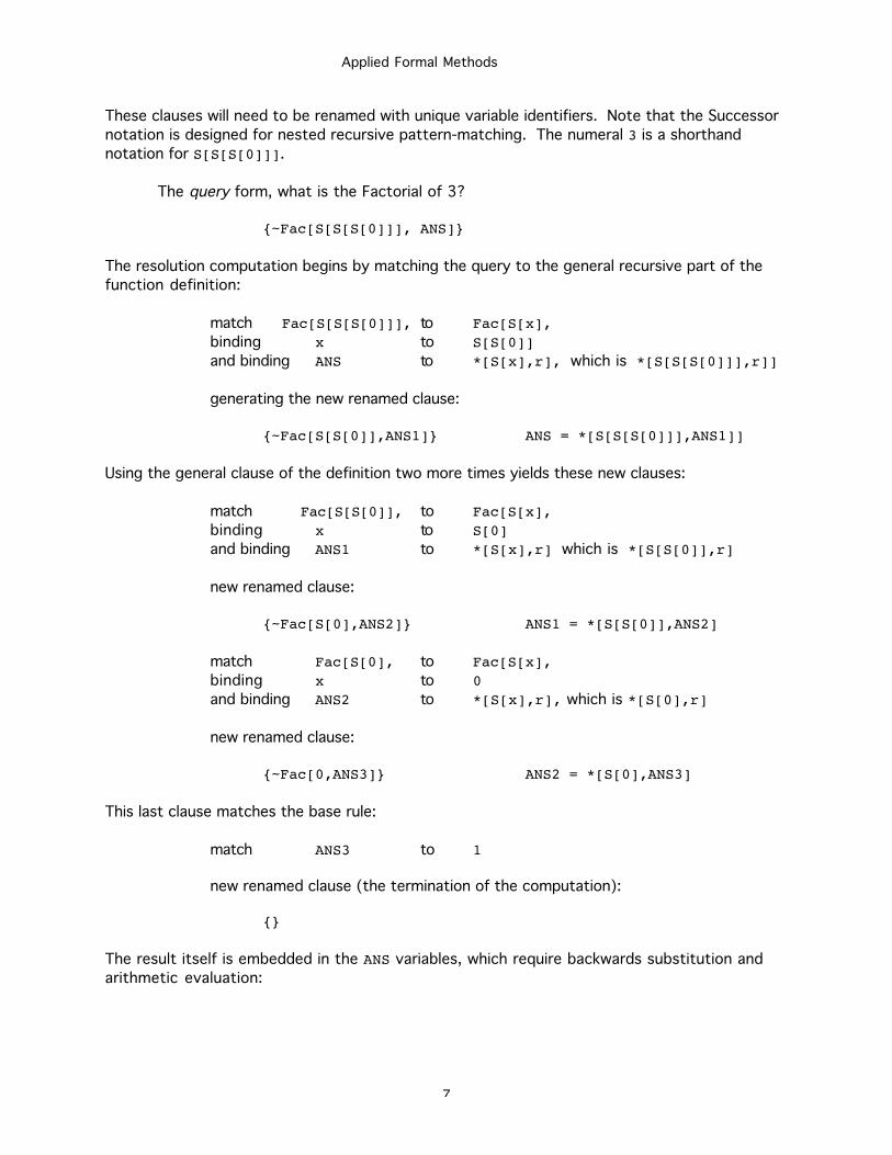
Applied Formal Methods
7
These clauses will need to be renamed with unique variable identifiers. Note that the Successor
notation is designed for nested recursive pattern-matching. The numeral 3 is a shorthand
notation for S[S[S[0]]].
The query form, what is the Factorial of 3?
{~Fac[S[S[S[0]]], ANS]}
The resolution computation begins by matching the query to the general recursive part of the
function definition:
match Fac[S[S[S[0]]], to Fac[S[x],binding x to S[S[0]]and binding ANS to *[S[x],r], which is *[S[S[S[0]]],r]]
generating the new renamed clause:
{~Fac[S[S[0]],ANS1]} ANS = *[S[S[S[0]]],ANS1]]
Using the general clause of the definition two more times yields these new clauses:
match Fac[S[S[0]], to Fac[S[x],binding x to S[0]and binding ANS1 to *[S[x],r] which is *[S[S[0]],r]
new renamed clause:
{~Fac[S[0],ANS2]} ANS1 = *[S[S[0]],ANS2]
match Fac[S[0], to Fac[S[x],binding x to 0and binding ANS2 to *[S[x],r], which is *[S[0],r]
new renamed clause:
{~Fac[0,ANS3]} ANS2 = *[S[0],ANS3]
This last clause matches the base rule:
match ANS3 to 1
new renamed clause (the termination of the computation):
{}
The result itself is embedded in the ANS variables, which require backwards substitution and
arithmetic evaluation:
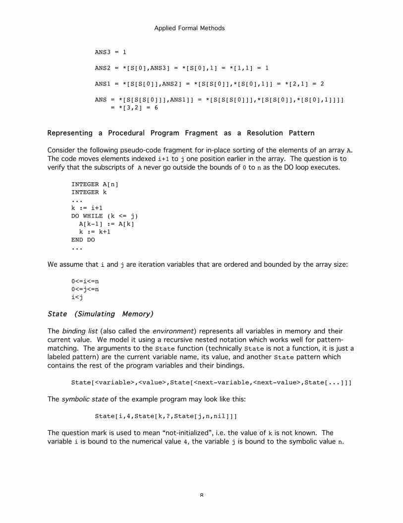
Applied Formal Methods
8
ANS3 = 1
ANS2 = *[S[0],ANS3] = *[S[0],1] = *[1,1] = 1
ANS1 = *[S[S[0]],ANS2] = *[S[S[0]],*[S[0],1]] = *[2,1] = 2
ANS = *[S[S[S[0]]],ANS1]] = *[S[S[S[0]]],*[S[S[0]],*[S[0],1]]]] = *[3,2] = 6
Representing a Procedural Program Fragment as a Resolution Pattern
Consider the following pseudo-code fragment for in-place sorting of the elements of an array A.
The code moves elements indexed i+1 to j one position earlier in the array. The question is to
verify that the subscripts of A never go outside the bounds of 0 to n as the DO loop executes.
INTEGER A[n]INTEGER k...k := i+1DO WHILE (k <= j) A[k-1] := A[k] k := k+1END DO...
We assume that i and j are iteration variables that are ordered and bounded by the array size:
0<=i<=n0<=j<=ni<j
State (Simulating Memory)
The binding list (also called the environment) represents all variables in memory and their
current value. We model it using a recursive nested notation which works well for pattern-
matching. The arguments to the State function (technically State is not a function, it is just a
labeled pattern) are the current variable name, its value, and another State pattern which
contains the rest of the program variables and their bindings.
State[<variable>,<value>,State[<next-variable,<next-value>,State[...]]]
The symbolic state of the example program may look like this:
State[i,4,State[k,?,State[j,n,nil]]]
The question mark is used to mean “not-initialized”, i.e. the value of k is not known. The
variable i is bound to the numerical value 4, the variable j is bound to the symbolic value n.
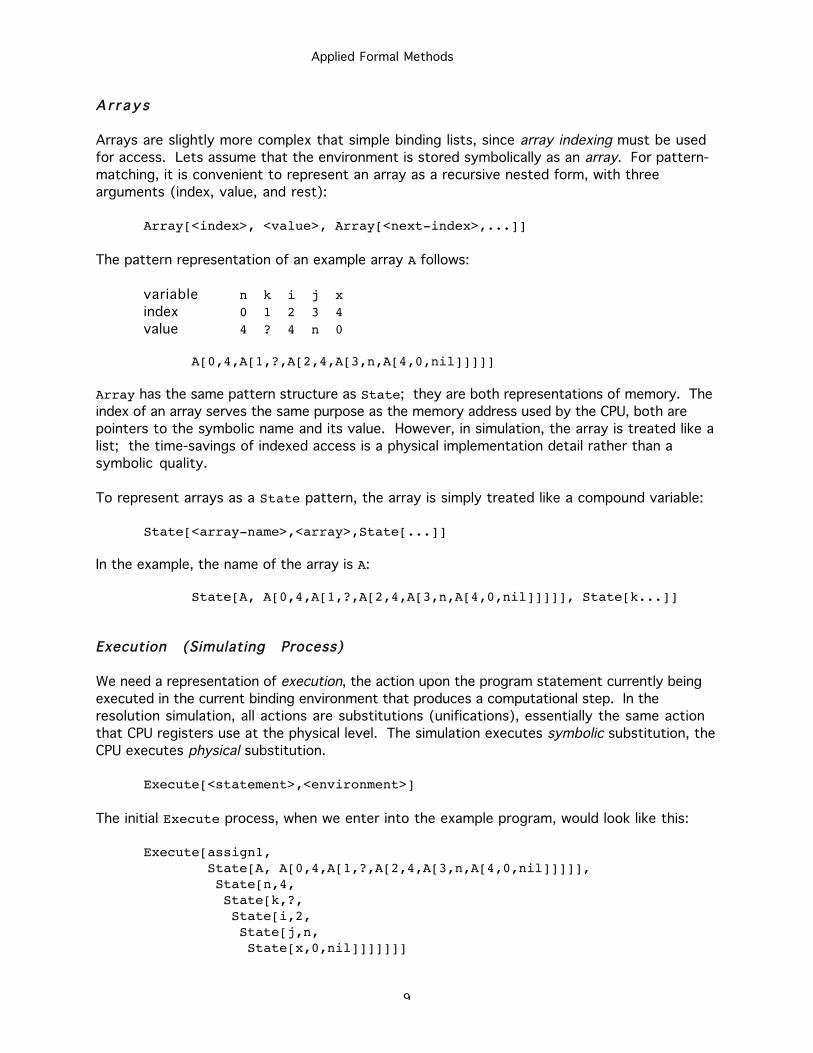
Applied Formal Methods
9
A r r a y s
Arrays are slightly more complex that simple binding lists, since array indexing must be used
for access. Lets assume that the environment is stored symbolically as an array. For pattern-
matching, it is convenient to represent an array as a recursive nested form, with three
arguments (index, value, and rest):
Array[<index>, <value>, Array[<next-index>,...]]
The pattern representation of an example array A follows:
variable n k i j xindex 0 1 2 3 4value 4 ? 4 n 0
A[0,4,A[1,?,A[2,4,A[3,n,A[4,0,nil]]]]]
Array has the same pattern structure as State; they are both representations of memory. The
index of an array serves the same purpose as the memory address used by the CPU, both are
pointers to the symbolic name and its value. However, in simulation, the array is treated like a
list; the time-savings of indexed access is a physical implementation detail rather than a
symbolic quality.
To represent arrays as a State pattern, the array is simply treated like a compound variable:
State[<array-name>,<array>,State[...]]
In the example, the name of the array is A:
State[A, A[0,4,A[1,?,A[2,4,A[3,n,A[4,0,nil]]]]], State[k...]]
Execution (Simulating Process)
We need a representation of execution, the action upon the program statement currently being
executed in the current binding environment that produces a computational step. In the
resolution simulation, all actions are substitutions (unifications), essentially the same action
that CPU registers use at the physical level. The simulation executes symbolic substitution, the
CPU executes physical substitution.
Execute[<statement>,<environment>]
The initial Execute process, when we enter into the example program, would look like this:
Execute[assign1, State[A, A[0,4,A[1,?,A[2,4,A[3,n,A[4,0,nil]]]]], State[n,4, State[k,?, State[i,2, State[j,n, State[x,0,nil]]]]]]]
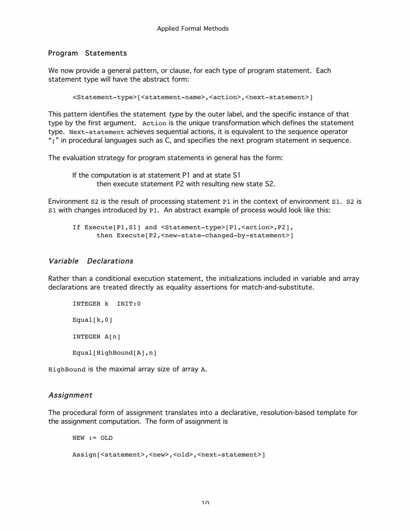
Applied Formal Methods
10
Program Statements
We now provide a general pattern, or clause, for each type of program statement. Each
statement type will have the abstract form:
<Statement-type>[<statement-name>,<action>,<next-statement>]
This pattern identifies the statement type by the outer label, and the specific instance of that
type by the first argument. Action is the unique transformation which defines the statement
type. Next-statement achieves sequential actions, it is equivalent to the sequence operator
“;” in procedural languages such as C, and specifies the next program statement in sequence.
The evaluation strategy for program statements in general has the form:
If the computation is at statement P1 and at state S1
then execute statement P2 with resulting new state S2.
Environment S2 is the result of processing statement P1 in the context of environment S1. S2 is
S1 with changes introduced by P1. An abstract example of process would look like this:
If Execute[P1,S1] and <Statement-type>[P1,<action>,P2],then Execute[P2,<new-state-changed-by-statement>]
Variable Declarations
Rather than a conditional execution statement, the initializations included in variable and array
declarations are treated directly as equality assertions for match-and-substitute.
INTEGER k INIT:0
Equal[k,0]
INTEGER A[n]
Equal[HighBound[A],n]
HighBound is the maximal array size of array A.
Assignment
The procedural form of assignment translates into a declarative, resolution-based template for
the assignment computation. The form of assignment is
NEW := OLD
Assign[<statement>,<new>,<old>,<next-statement>]
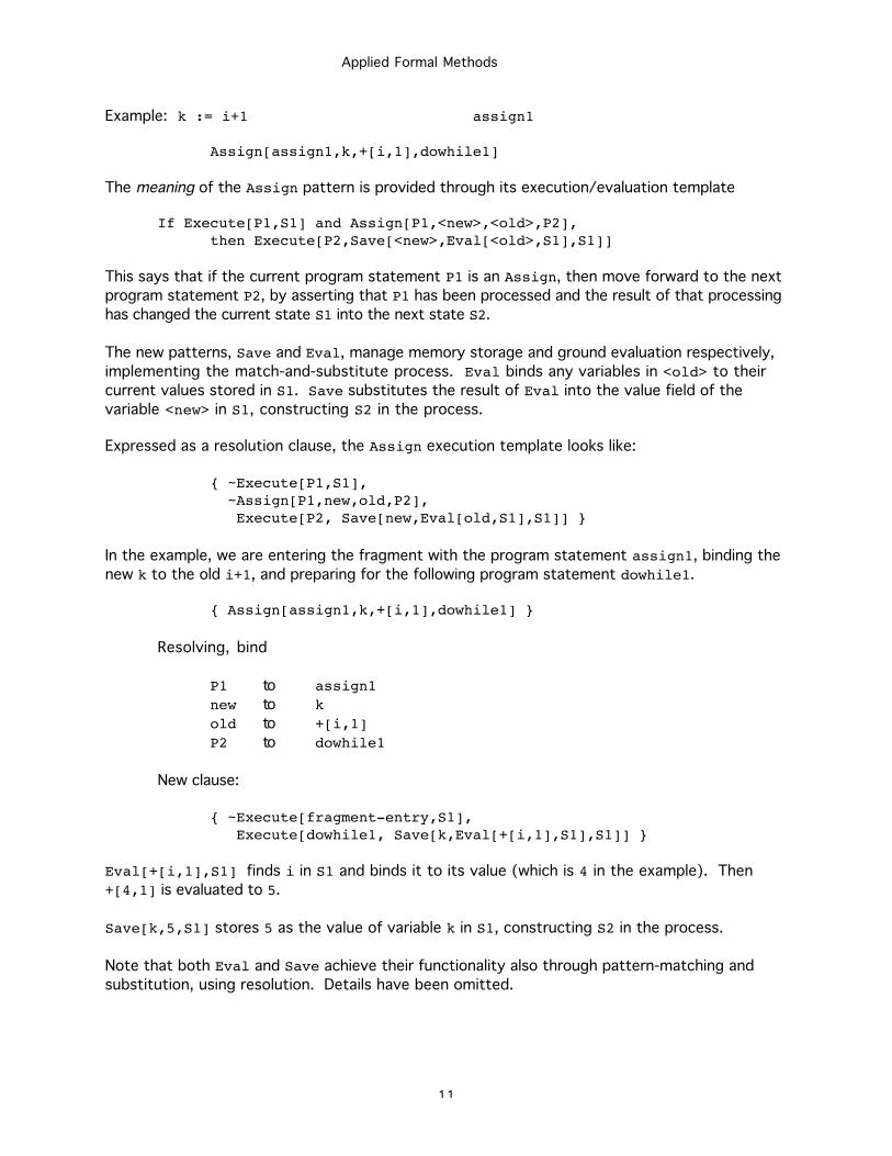
Applied Formal Methods
11
Example: k := i+1 assign1
Assign[assign1,k,+[i,1],dowhile1]
The meaning of the Assign pattern is provided through its execution/evaluation template
If Execute[P1,S1] and Assign[P1,<new>,<old>,P2],then Execute[P2,Save[<new>,Eval[<old>,S1],S1]]
This says that if the current program statement P1 is an Assign, then move forward to the next
program statement P2, by asserting that P1 has been processed and the result of that processing
has changed the current state S1 into the next state S2.
The new patterns, Save and Eval, manage memory storage and ground evaluation respectively,
implementing the match-and-substitute process. Eval binds any variables in <old> to their
current values stored in S1. Save substitutes the result of Eval into the value field of the
variable <new> in S1, constructing S2 in the process.
Expressed as a resolution clause, the Assign execution template looks like:
{ ~Execute[P1,S1], ~Assign[P1,new,old,P2], Execute[P2, Save[new,Eval[old,S1],S1]] }
In the example, we are entering the fragment with the program statement assign1, binding the
new k to the old i+1, and preparing for the following program statement dowhile1.
{ Assign[assign1,k,+[i,1],dowhile1] }
Resolving, bind
P1 to assign1new to kold to +[i,1]P2 to dowhile1
New clause:
{ ~Execute[fragment-entry,S1], Execute[dowhile1, Save[k,Eval[+[i,1],S1],S1]] }
Eval[+[i,1],S1] finds i in S1 and binds it to its value (which is 4 in the example). Then
+[4,1] is evaluated to 5.
Save[k,5,S1] stores 5 as the value of variable k in S1, constructing S2 in the process.
Note that both Eval and Save achieve their functionality also through pattern-matching and
substitution, using resolution. Details have been omitted.
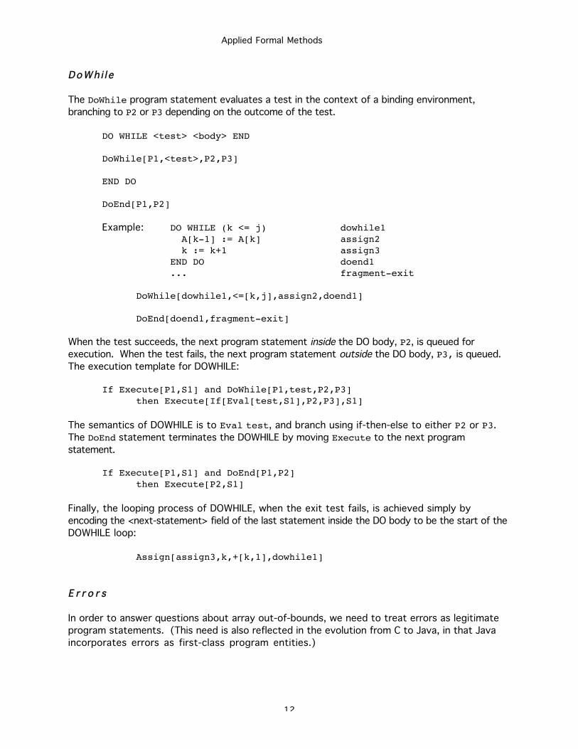
Applied Formal Methods
12
DoWh i l e
The DoWhile program statement evaluates a test in the context of a binding environment,
branching to P2 or P3 depending on the outcome of the test.
DO WHILE <test> <body> END
DoWhile[P1,<test>,P2,P3]
END DO
DoEnd[P1,P2]
Example: DO WHILE (k <= j) dowhile1 A[k-1] := A[k] assign2 k := k+1 assign3END DO doend1... fragment-exit
DoWhile[dowhile1,<=[k,j],assign2,doend1]
DoEnd[doend1,fragment-exit]
When the test succeeds, the next program statement inside the DO body, P2, is queued for
execution. When the test fails, the next program statement outside the DO body, P3, is queued.
The execution template for DOWHILE:
If Execute[P1,S1] and DoWhile[P1,test,P2,P3]then Execute[If[Eval[test,S1],P2,P3],S1]
The semantics of DOWHILE is to Eval test, and branch using if-then-else to either P2 or P3.
The DoEnd statement terminates the DOWHILE by moving Execute to the next program
statement.
If Execute[P1,S1] and DoEnd[P1,P2]then Execute[P2,S1]
Finally, the looping process of DOWHILE, when the exit test fails, is achieved simply by
encoding the <next-statement> field of the last statement inside the DO body to be the start of the
DOWHILE loop:
Assign[assign3,k,+[k,1],dowhile1]
E r r o r s
In order to answer questions about array out-of-bounds, we need to treat errors as legitimate
program statements. (This need is also reflected in the evolution from C to Java, in that Java
incorporates errors as first-class program entities.)
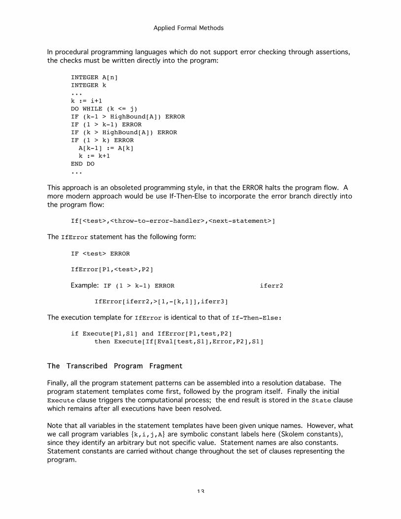
Applied Formal Methods
13
In procedural programming languages which do not support error checking through assertions,
the checks must be written directly into the program:
INTEGER A[n]INTEGER k...k := i+1DO WHILE (k <= j)IF (k-1 > HighBound[A]) ERRORIF (1 > k-1) ERRORIF (k > HighBound[A]) ERRORIF (1 > k) ERROR A[k-1] := A[k] k := k+1END DO...
This approach is an obsoleted programming style, in that the ERROR halts the program flow. A
more modern approach would be use If-Then-Else to incorporate the error branch directly into
the program flow:
If[<test>,<throw-to-error-handler>,<next-statement>]
The IfError statement has the following form:
IF <test> ERROR
IfError[P1,<test>,P2]
Example: IF (1 > k-1) ERROR iferr2
IfError[iferr2,>[1,-[k,1]],iferr3]
The execution template for IfError is identical to that of If-Then-Else:
if Execute[P1,S1] and IfError[P1,test,P2]then Execute[If[Eval[test,S1],Error,P2],S1]
The Transcribed Program Fragment
Finally, all the program statement patterns can be assembled into a resolution database. The
program statement templates come first, followed by the program itself. Finally the initial
Execute clause triggers the computational process; the end result is stored in the State clause
which remains after all executions have been resolved.
Note that all variables in the statement templates have been given unique names. However, what
we call program variables {k,i,j,A} are symbolic constant labels here (Skolem constants),
since they identify an arbitrary but not specific value. Statement names are also constants.
Statement constants are carried without change throughout the set of clauses representing the
program.
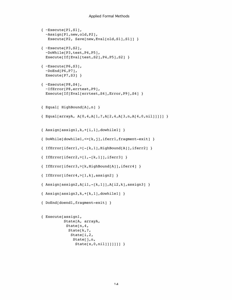
Applied Formal Methods
14
{ ~Execute[P1,S1], ~Assign[P1,new,old,P2], Execute[P2, Save[new,Eval[old,S1],S1]] }
{ ~Execute[P3,S2], ~DoWhile[P3,test,P4,P5], Execute[If[Eval[test,S2],P4,P5],S2] }
{ ~Execute[P6,S3], ~DoEnd[P6,P7], Execute[P7,S3] }
{ ~Execute[P8,S4], ~IfError[P8,errtest,P9], Execute[If[Eval[errtest,S4],Error,P9],S4] }
{ Equal[ HighBound[A],n] }
{ Equal[arrayA, A[0,4,A[1,?,A[2,4,A[3,n,A[4,0,nil]]]]] }
{ Assign[assign1,k,+[i,1],dowhile1] }
{ DoWhile[dowhile1,<=[k,j],iferr1,fragment-exit] }
{ IfError[iferr1,>[-[k,1],HighBound[A]],iferr2] }
{ IfError[iferr2,>[1,-[k,1]],iferr3] }
{ IfError[iferr3,>[k,HighBound[A]],iferr4] }
{ IfError[iferr4,>[1,k],assign2] }
{ Assign[assign2,A[i1,-[k,1]],A[i2,k],assign3] }
{ Assign[assign3,k,+[k,1],dowhile1] }
{ DoEnd[doend1,fragment-exit] }
{ Execute[assign1, State[A, arrayA, State[n,4, State[k,?, State[i,2, State[j,n, State[x,0,nil]]]]]]] }
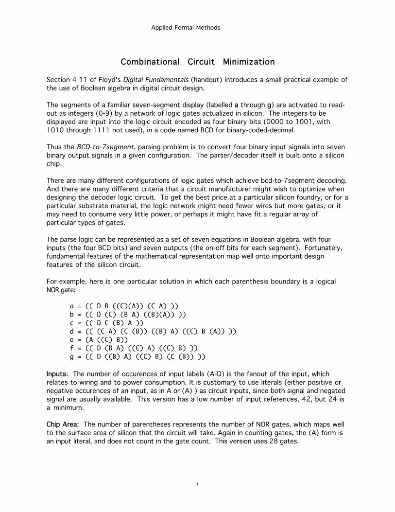
Applied Formal Methods
1
Combinational Circuit Minimization
Section 4-11 of Floyd's Digital Fundamentals (handout) introduces a small practical example of
the use of Boolean algebra in digital circuit design.
The segments of a familiar seven-segment display (labelled aa through gg) are activated to read-
out as integers (0-9) by a network of logic gates actualized in silicon. The integers to be
displayed are input into the logic circuit encoded as four binary bits (0000 to 1001, with
1010 through 1111 not used), in a code named BCD for binary-coded-decimal.
Thus the BCD-to-7segment. parsing problem is to convert four binary input signals into seven
binary output signals in a given configuration. The parser/decoder itself is built onto a silicon
chip.
There are many different configurations of logic gates which achieve bcd-to-7segment decoding.
And there are many different criteria that a circuit manufacturer might wish to optimize when
designing the decoder logic circuit. To get the best price at a particular silicon foundry, or for a
particular substrate material, the logic network might need fewer wires but more gates, or it
may need to consume very little power, or perhaps it might have fit a regular array of
particular types of gates.
The parse logic can be represented as a set of seven equations in Boolean algebra, with four
inputs (the four BCD bits) and seven outputs (the on-off bits for each segment). Fortunately,
fundamental features of the mathematical representation map well onto important design
features of the silicon circuit.
For example, here is one particular solution in which each parenthesis boundary is a logical
NOR gate:
a = (( D B ((C)(A)) (C A) ))
b = (( D (C) (B A) ((B)(A)) ))
c = (( D C (B) A ))
d = (( (C A) (C (B)) ((B) A) ((C) B (A)) ))
e = (A ((C) B))
f = (( D (B A) ((C) A) ((C) B) ))
g = (( D ((B) A) ((C) B) (C (B)) ))
Inputs: The number of occurences of input labels (A-D) is the fanout of the input, which
relates to wiring and to power consumption. It is customary to use literals (either positive or
negative occurences of an input, as in A or (A) ) as circuit inputs, since both signal and negated
signal are usually available. This version has a low number of input references, 42, but 24 is
a minimum.
Chip Area: The number of parentheses represents the number of NOR gates, which maps well
to the surface area of silicon that the circuit will take. Again in counting gates, the (A) form is
an input literal, and does not count in the gate count. This version uses 28 gates.
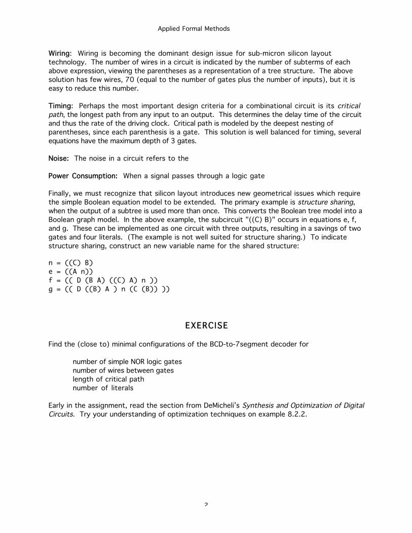
Applied Formal Methods
2
Wiring: Wiring is becoming the dominant design issue for sub-micron silicon layout
technology. The number of wires in a circuit is indicated by the number of subterms of each
above expression, viewing the parentheses as a representation of a tree structure. The above
solution has few wires, 70 (equal to the number of gates plus the number of inputs), but it is
easy to reduce this number.
Timing: Perhaps the most important design criteria for a combinational circuit is its criticalpath, the longest path from any input to an output. This determines the delay time of the circuit
and thus the rate of the driving clock. Critical path is modeled by the deepest nesting of
parentheses, since each parenthesis is a gate. This solution is well balanced for timing, several
equations have the maximum depth of 3 gates.
Noise: The noise in a circuit refers to the
Power Consumption: When a signal passes through a logic gate
Finally, we must recognize that silicon layout introduces new geometrical issues which require
the simple Boolean equation model to be extended. The primary example is structure sharing,
when the output of a subtree is used more than once. This converts the Boolean tree model into a
Boolean graph model. In the above example, the subcircuit "((C) B)" occurs in equations e, f,
and g. These can be implemented as one circuit with three outputs, resulting in a savings of two
gates and four literals. (The example is not well suited for structure sharing.) To indicate
structure sharing, construct an new variable name for the shared structure:
n = ((C) B)
e = ((A n))
f = (( D (B A) ((C) A) n ))
g = (( D ((B) A ) n (C (B)) ))
EXERCISE
Find the (close to) minimal configurations of the BCD-to-7segment decoder for
number of simple NOR logic gates
number of wires between gates
length of critical path
number of literals
Early in the assignment, read the section from DeMicheli’s Synthesis and Optimization of DigitalCircuits. Try your understanding of optimization techniques on example 8.2.2.
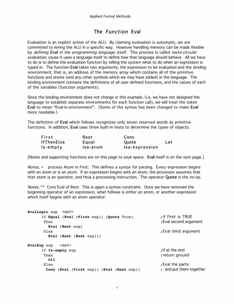
Applied Formal Methods
1
The Function Eval
Evaluation is an implicit action of the ALU. By claiming evaluation is automatic, we are
committed to wiring the ALU in a specific way. However handling memory can be made flexible
by defining EEval in the programming language itself. This process is called meta-circularevaluation, cause it uses a language itself to define how that language should behave. All we have
to do is to define the evaluation function by telling the system what to do when an expression is
typed in. The function EEval takes two arguments, the expression to be evaluated and the bindingenvironment, that is, an address of the memory array which contains all of the primitive
functions and atoms (and any other symbols which we may have added) in the language. The
binding environment contains the definitions of all user defined functions, and the values of each
of the variables (function arguments).
Since the binding environment does not change in this example, (i.e. we have not designed the
language to establish separate environments for each function call), we will treat the token
Eval to mean “Eval-in-environment”. (Some of the syntax has been changed to make EEval
more readable.)
The definition of EEval which follows recognizes only seven reserved words as primitive
functions. In addition, EEval uses three built-in tests to determine the types of objects.
F i r s t Rest Cons
I fThenE lse Equa l Quote Let
I s - e m p t y I sa -a tom I sa - exp res s i on
[Notes and supporting functions are on this page to save space. EEval itself is on the next page.]
Notes, * process Atom in First: This defines a syntax for parsing. Every expression begins
with an atom or is an atom. If an expression begins with an atom, the processor assumes that
that atom is an operator, and thus a processing instruction. The operator QQuote is the no-op.
Notes, ** Cons Eval of Rest: This is again a syntax constraint. Once we have removed the
beginning operator of an expression, what follows is either an atom, or another expression
which itself begins with an atom operator.
EvalLogic exp =def=If Equal (Eval (First exp)) (Quote True) ;if First is TRUE
Then ;Eval second argument Eval (Rest exp) Else ;Eval third argument Eval (Rest (Rest exp)))
EvalExp exp =def=If Is-empty exp ;if at the end
Then ;return ground nil Else ;Eval the parts
Cons (Eval (First exp)) (Eval (Rest exp)) ; and put them together
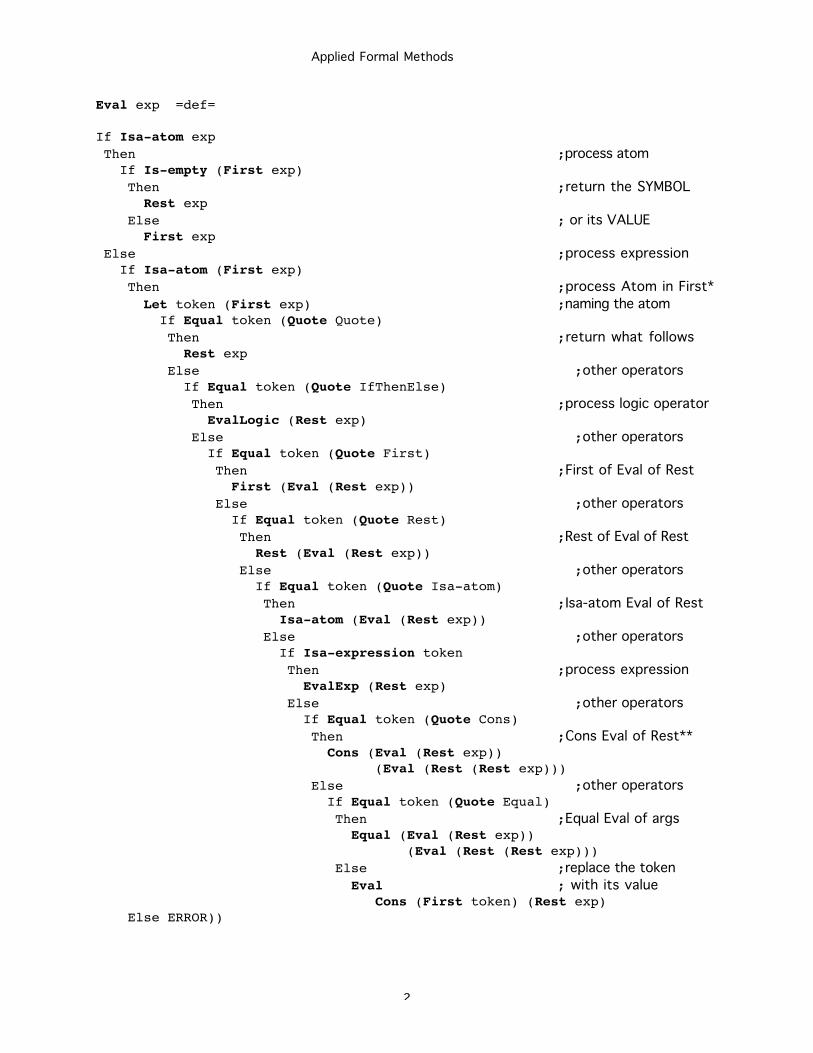
Applied Formal Methods
2
Eval exp =def=
If Isa-atom exp Then ;process atom If Is-empty (First exp) Then ;return the SYMBOL Rest exp Else ; or its VALUE First exp Else ;process expression If Isa-atom (First exp) Then ;process Atom in First*
Let token (First exp) ;naming the atom If Equal token (Quote Quote) Then ;return what follows Rest exp Else ;other operators If Equal token (Quote IfThenElse) Then ;process logic operator EvalLogic (Rest exp) Else ;other operators If Equal token (Quote First) Then ;First of Eval of Rest First (Eval (Rest exp)) Else ;other operators If Equal token (Quote Rest) Then ;Rest of Eval of Rest Rest (Eval (Rest exp)) Else ;other operators If Equal token (Quote Isa-atom) Then ;Isa-atom Eval of Rest Isa-atom (Eval (Rest exp)) Else ;other operators If Isa-expression token Then ;process expression EvalExp (Rest exp) Else ;other operators If Equal token (Quote Cons) Then ;Cons Eval of Rest** Cons (Eval (Rest exp)) (Eval (Rest (Rest exp))) Else ;other operators If Equal token (Quote Equal) Then ;Equal Eval of args Equal (Eval (Rest exp)) (Eval (Rest (Rest exp))) Else ;replace the token
Eval ; with its value Cons (First token) (Rest exp) Else ERROR))
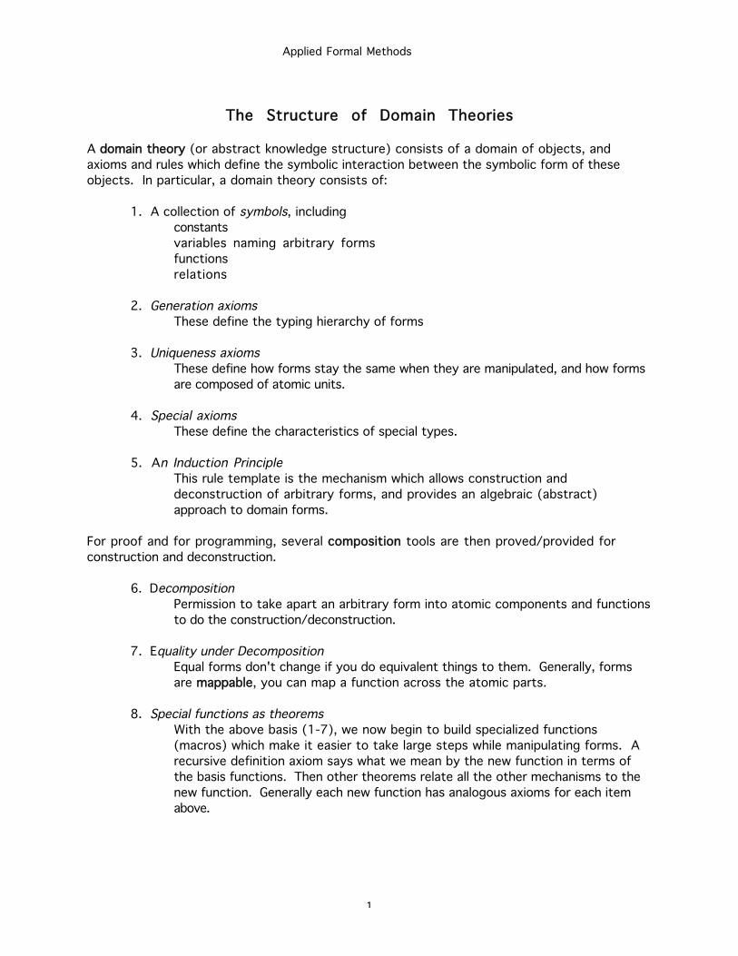
Applied Formal Methods
1
The Structure of Domain Theories
A ddomain theory (or abstract knowledge structure) consists of a domain of objects, and
axioms and rules which define the symbolic interaction between the symbolic form of these
objects. In particular, a domain theory consists of:
1. A collection of symbols, including
constants
variables naming arbitrary forms
functions
relations
2. Generation axiomsThese define the typing hierarchy of forms
3. Uniqueness axiomsThese define how forms stay the same when they are manipulated, and how forms
are composed of atomic units.
4. Special axiomsThese define the characteristics of special types.
5. An Induction PrincipleThis rule template is the mechanism which allows construction and
deconstruction of arbitrary forms, and provides an algebraic (abstract)
approach to domain forms.
For proof and for programming, several ccomposition tools are then proved/provided for
construction and deconstruction.
6. DecompositionPermission to take apart an arbitrary form into atomic components and functions
to do the construction/deconstruction.
7. Equality under DecompositionEqual forms don't change if you do equivalent things to them. Generally, forms
are mmappable, you can map a function across the atomic parts.
8. Special functions as theoremsWith the above basis (1-7), we now begin to build specialized functions
(macros) which make it easier to take large steps while manipulating forms. A
recursive definition axiom says what we mean by the new function in terms of
the basis functions. Then other theorems relate all the other mechanisms to the
new function. Generally each new function has analogous axioms for each item
above.
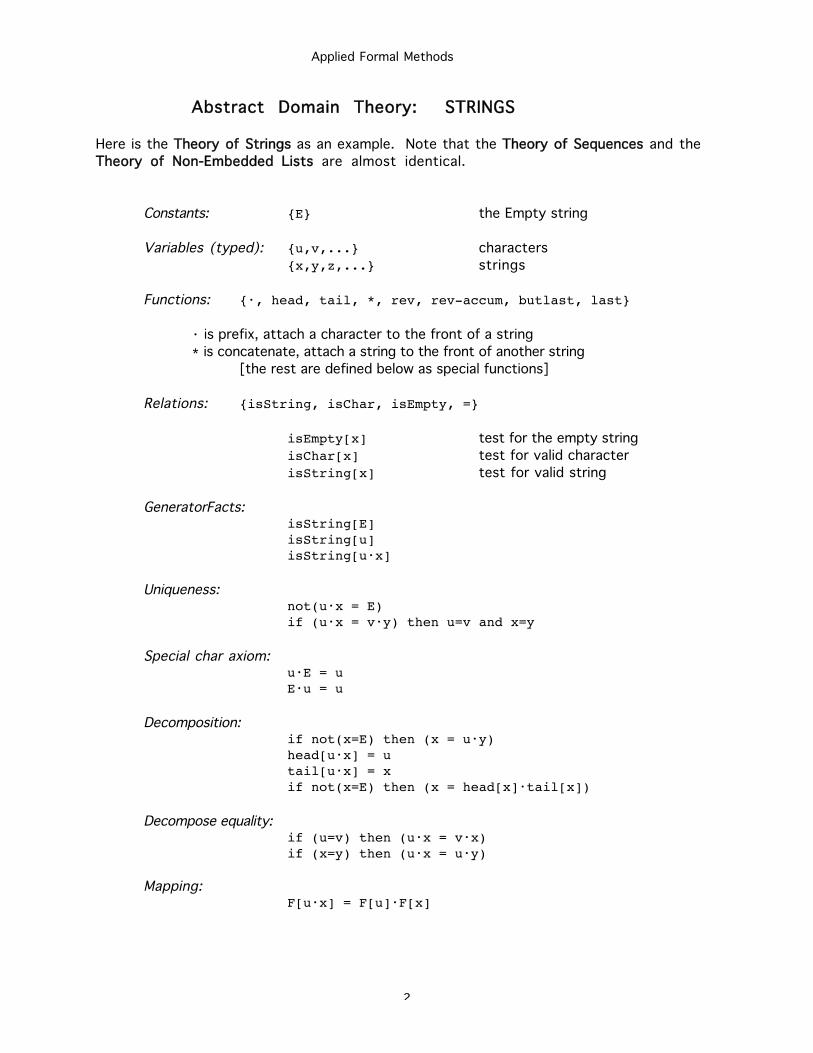
Applied Formal Methods
2
Abstract Domain Theory: STRINGS
Here is the TTheory of Strings as an example. Note that the TTheory of Sequences and the
Theory of Non-Embedded Lists are almost identical.
Constants: {E} the Empty string
Variables (typed): {u,v,...} characters
{x,y,z,...} strings
Functions: {•, head, tail, *, rev, rev-accum, butlast, last}
• is prefix, attach a character to the front of a string
* is concatenate, attach a string to the front of another string
[the rest are defined below as special functions]
Relations: {isString, isChar, isEmpty, =}
isEmpty[x] test for the empty string
isChar[x] test for valid character
isString[x] test for valid string
GeneratorFacts:isString[E]isString[u]isString[u•x]
Uniqueness:not(u•x = E)if (u•x = v•y) then u=v and x=y
Special char axiom:u•E = uE•u = u
Decomposition:if not(x=E) then (x = u•y)head[u•x] = utail[u•x] = xif not(x=E) then (x = head[x]•tail[x])
Decompose equality:if (u=v) then (u•x = v•x)if (x=y) then (u•x = u•y)
Mapping:F[u•x] = F[u]•F[x]
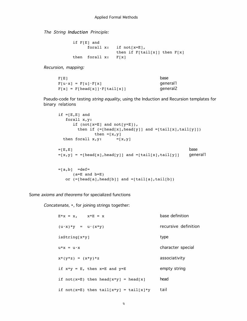
Applied Formal Methods
3
The String IInduction Principle:
if F[E] andforall x: if not[x=E],
then if F[tail[x]] then F[x]then forall x: F[x]
Recursion, mapping:
F[E] base
F[u•x] = F[u]•F[x] general1
F[x] = F[head[x]]•F[tail[x]] general2
Pseudo-code for testing string equality, using the Induction and Recursion templates for
binary relations
if =[E,E] and forall x,y:
if (not[x=E] and not[y=E]), then if (=[head[x],head[y]] and =[tail[x],tail[y]])
then =[x,y] then forall x,y: =[x,y]
=[E,E] base
=[x,y] = =[head[x],head[y]] and =[tail[x],tail[y]] general1
=[a,b] =def=(a=E and b=E)
or (=[head[a],head[b]] and =[tail[a],tail[b])
Some axioms and theorems for specialized functions
Concatenate, *, for joining strings together:
E*x = x, x*E = x base definition
(u•x)*y = u•(x*y) recursive definition
isString[x*y] type
u*x = u•x character special
x*(y*z) = (x*y)*z associativity
if x*y = E, then x=E and y=E empty string
if not(x=E) then head[x*y] = head[x] head
if not(x=E) then tail[x*y] = tail[x]*y tail
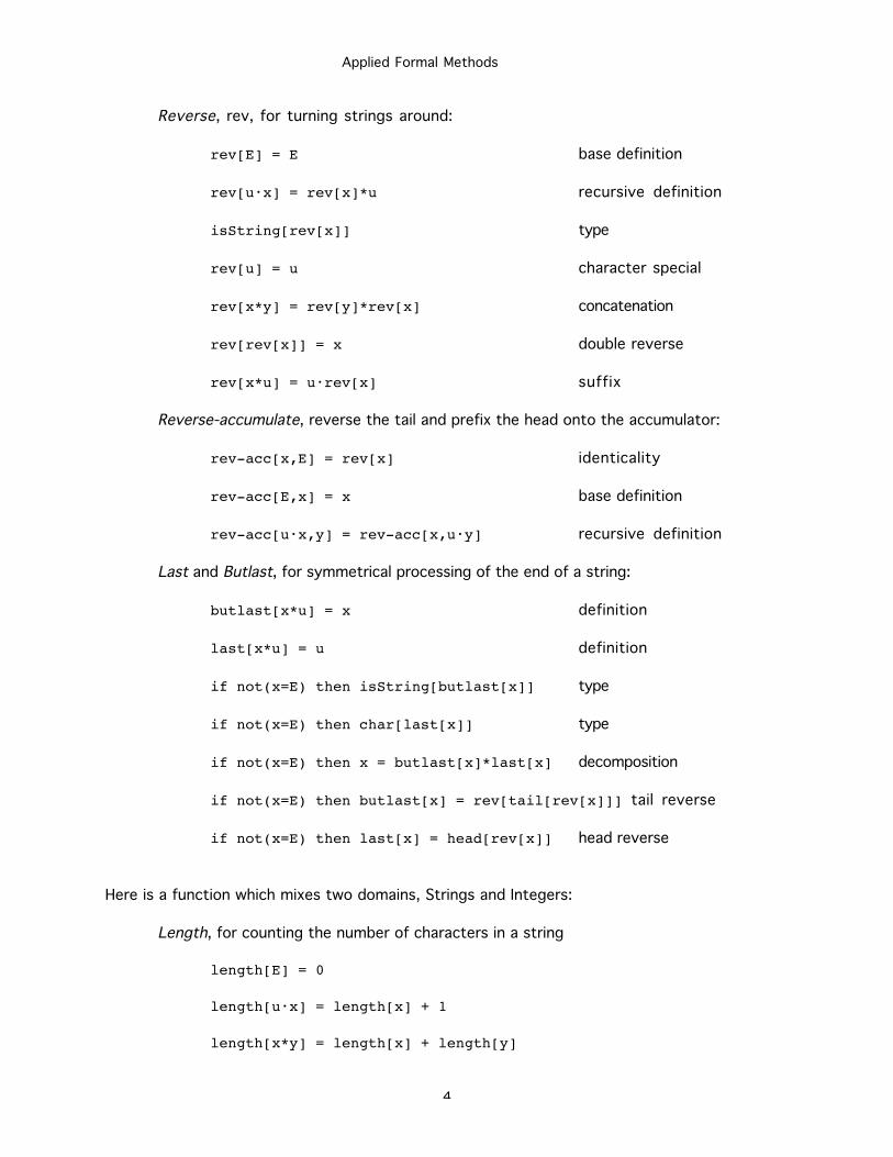
Applied Formal Methods
4
Reverse, rev, for turning strings around:
rev[E] = E base definition
rev[u•x] = rev[x]*u recursive definition
isString[rev[x]] type
rev[u] = u character special
rev[x*y] = rev[y]*rev[x] concatenation
rev[rev[x]] = x double reverse
rev[x*u] = u•rev[x] suffix
Reverse-accumulate, reverse the tail and prefix the head onto the accumulator:
rev-acc[x,E] = rev[x] identicality
rev-acc[E,x] = x base definition
rev-acc[u•x,y] = rev-acc[x,u•y] recursive definition
Last and Butlast, for symmetrical processing of the end of a string:
butlast[x*u] = x definition
last[x*u] = u definition
if not(x=E) then isString[butlast[x]] type
if not(x=E) then char[last[x]] type
if not(x=E) then x = butlast[x]*last[x] decomposition
if not(x=E) then butlast[x] = rev[tail[rev[x]]] tail reverse
if not(x=E) then last[x] = head[rev[x]] head reverse
Here is a function which mixes two domains, Strings and Integers:
Length, for counting the number of characters in a string
length[E] = 0
length[u•x] = length[x] + 1
length[x*y] = length[x] + length[y]
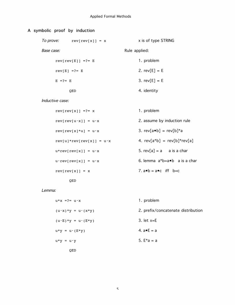
Applied Formal Methods
5
A symbolic proof by induction
To prove: rev[rev[x]] = x x is of type STRING
Base case: Rule applied:
rev[rev[E]] =?= E 1. problem
rev[E] =?= E 2. rev[E] = E
E =?= E 3. rev[E] = E
QED 4. identity
Inductive case:
rev[rev[x]] =?= x 1. problem
rev[rev[u•x]] = u•x 2. assume by induction rule
rev[rev[x]*u] = u•x 3. rev[a•b] = rev[b]*a
rev[u]*rev[rev[x]] = u•x 4. rev[a*b] = rev[b]*rev[a]
u*rev[rev[x]] = u•x 5. rev[a] = a a is a char
u•rev[rev[x]] = u•x 6. lemma a*b=a•b a is a char
rev[rev[x]] = x 7. a•b = a•c iff b=c
QED
Lemma:
u*x =?= u•x 1. problem
(u•x)*y = u•(x*y) 2. prefix/concatenate distribution
(u•E)*y = u•(E*y) 3. let x=E
u*y = u•(E*y) 4. a•E = a
u*y = u•y 5. E*a = a
QED
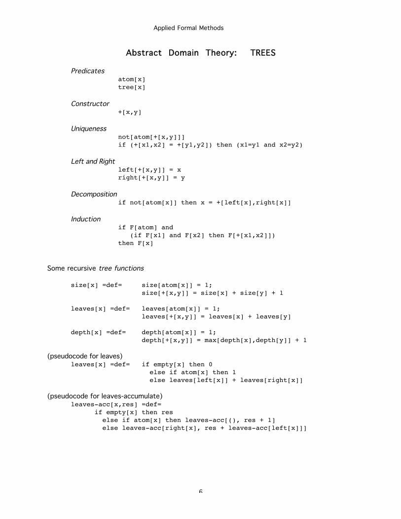
Applied Formal Methods
6
Abstract Domain Theory: TREES
Predicatesatom[x]tree[x]
Constructor+[x,y]
Uniquenessnot[atom[+[x,y]]]if (+[x1,x2] = +[y1,y2]) then (x1=y1 and x2=y2)
Left and Rightleft[+[x,y]] = xright[+[x,y]] = y
Decompositionif not[atom[x]] then x = +[left[x],right[x]]
Inductionif F[atom] and (if F[x1] and F[x2] then F[+[x1,x2]])then F[x]
Some recursive tree functions
size[x] =def= size[atom[x]] = 1;size[+[x,y]] = size[x] + size[y] + 1
leaves[x] =def= leaves[atom[x]] = 1;leaves[+[x,y]] = leaves[x] + leaves[y]
depth[x] =def= depth[atom[x]] = 1;depth[+[x,y]] = max[depth[x],depth[y]] + 1
(pseudocode for leaves)leaves[x] =def= if empty[x] then 0
else if atom[x] then 1 else leaves[left[x]] + leaves[right[x]]
(pseudocode for leaves-accumulate)leaves-acc[x,res] =def=
if empty[x] then res else if atom[x] then leaves-acc[(), res + 1] else leaves-acc[right[x], res + leaves-acc[left[x]]]
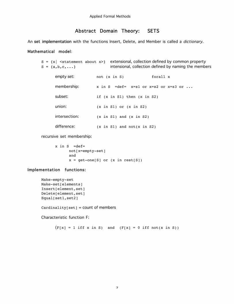
Applied Formal Methods
7
Abstract Domain Theory: SETS
An sset implementation with the functions Insert, Delete, and Member is called a dictionary.
Mathematical model:
S = {x| <statement about x>} extensional, collection defined by common property
S = {a,b,c,...} intensional, collection defined by naming the members
empty set: not (x in S) forall x
membership: x in S =def= x=s1 or x=s2 or x=s3 or ...
subset: if (x in S1) then (x in S2)
union: (x in S1) or (x in S2)
intersection: (x in S1) and (x in S2)
difference: (x in S1) and not(x in S2)
recursive set membership:
x in S =def=not[x=empty-set]andx = get-one[S] or (x in rest[S])
Implementation functions:
Make-empty-setMake-set[elements]Insert[element,set]Delete[element,set]Equal[set1,set2]
Cardinality[set] = count of members
Characteristic function F:
(F[x] = 1 iff x in S) and (F[x] = 0 iff not(x in S))
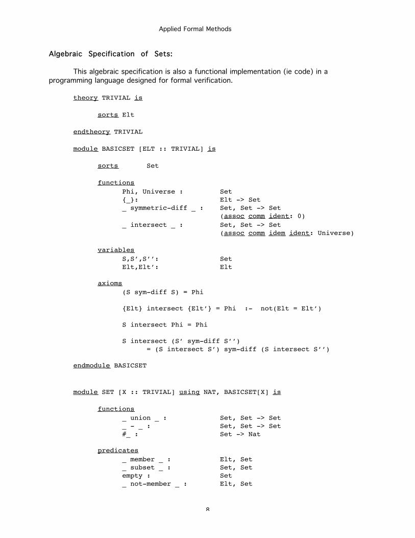
Applied Formal Methods
8
Algebraic Specification of Sets:
This algebraic specification is also a functional implementation (ie code) in a
programming language designed for formal verification.
theory TRIVIAL is
sorts Elt
endtheory TRIVIAL
module BASICSET [ELT :: TRIVIAL] is
sorts Set
functions Phi, Universe : Set{_}: Elt -> Set_ symmetric-diff _ : Set, Set -> Set
( assoc comm ident : 0)_ intersect _ : Set, Set -> Set
( assoc comm idem ident : Universe)
variables S,S’,S’’: SetElt,Elt’: Elt
axioms (S sym-diff S) = Phi
{Elt} intersect {Elt’} = Phi :- not(Elt = Elt’)
S intersect Phi = Phi
S intersect (S’ sym-diff S’’)= (S intersect S’) sym-diff (S intersect S’’)
endmodule BASICSET
module SET [X :: TRIVIAL] using NAT, BASICSET[X] is
functions _ union _ : Set, Set -> Set_ - _ : Set, Set -> Set#_ : Set -> Nat
predicates_ member _ : Elt, Set_ subset _ : Set, Setempty : Set_ not-member _ : Elt, Set
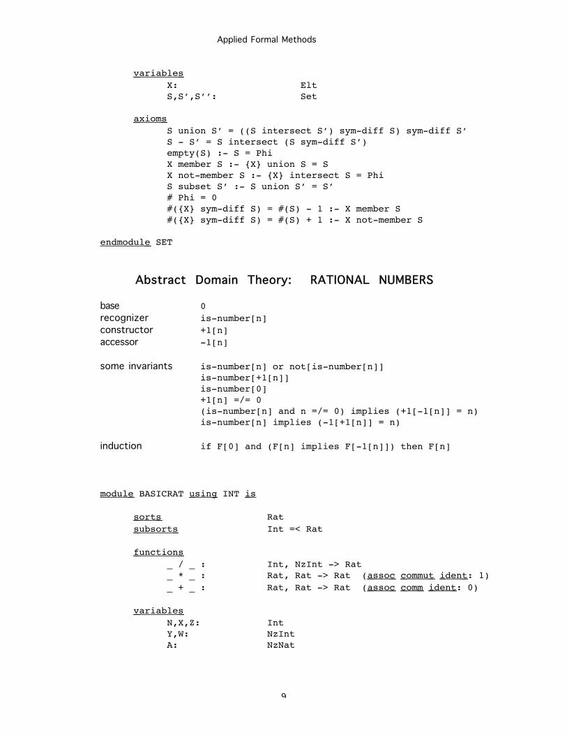
Applied Formal Methods
9
variables X: EltS,S’,S’’: Set
axioms S union S’ = ((S intersect S’) sym-diff S) sym-diff S’S - S’ = S intersect (S sym-diff S’)empty(S) :- S = PhiX member S :- {X} union S = SX not-member S :- {X} intersect S = PhiS subset S’ :- S union S’ = S’# Phi = 0#({X} sym-diff S) = #(S) - 1 :- X member S#({X} sym-diff S) = #(S) + 1 :- X not-member S
endmodule SET
Abstract Domain Theory: RATIONAL NUMBERS
base 0recognizer is-number[n]constructor +1[n]accessor -1[n]
some invariants is-number[n] or not[is-number[n]]is-number[+1[n]]is-number[0]+1[n] =/= 0(is-number[n] and n =/= 0) implies (+1[-1[n]] = n)is-number[n] implies (-1[+1[n]] = n)
induction if F[0] and (F[n] implies F[-1[n]]) then F[n]
module BASICRAT using INT is
sorts Rat subsorts Int =< Rat
functions _ / _ : Int, NzInt -> Rat_ * _ : Rat, Rat -> Rat ( assoc commut ident : 1)_ + _ : Rat, Rat -> Rat ( assoc comm ident : 0)
variables N,X,Z: IntY,W: NzIntA: NzNat
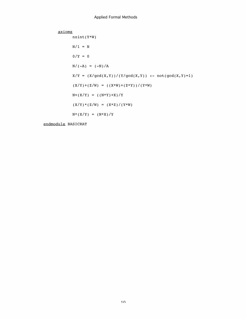
Applied Formal Methods
10
axioms nzint(Y*W)
N/1 = N
0/Y = 0
N/(-A) = (-N)/A
X/Y = (X/gcd(X,Y))/(Y/gcd(X,Y)) :- not(gcd(X,Y)=1)
(X/Y)+(Z/W) = ((X*W)+(Z*Y))/(Y*W)
N+(X/Y) = ((N*Y)+X)/Y
(X/Y)*(Z/W) = (X*Z)/(Y*W)
N*(X/Y) = (N*X)/Y
endmodule BASICRAT
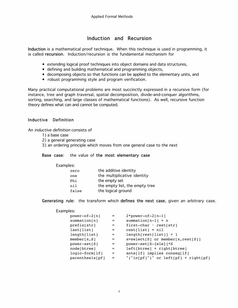
Applied Formal Methods
1
Induction and Recursion
Induction is a mathematical proof technique. When this technique is used in programming, it
is called rrecursion. Induction/recursion is the fundamental mechanism for
• extending logical proof techniques into object domains and data structures,
• defining and building mathematical and programming objects,
• decomposing objects so that functions can be applied to the elementary units, and
• robust programming style and program verification.
Many practical computational problems are most succinctly expressed in a recursive form (for
instance, tree and graph traversal, spatial decomposition, divide-and-conquer algorithms,
sorting, searching, and large classes of mathematical functions). As well, recursive function
theory defines what can and cannot be computed.
Inductive Definition
An inductive definition consists of
1) a base case
2) a general generating case
3) an ordering principle which moves from one general case to the next
Base case: the value of tthe most elementary case
Examples:
zero the additive identity
one the multiplicative identity
Phi the empty set
nil the empty list, the empty tree
false the logical ground
Generating rule: the transform which ddefines the next case, given an arbitrary case.
Examples:power-of-2[n] = 2*power-of-2[n-1]summation[n] = summation[n-1] + nprefix[str] = first-char • rest[str]last[list] = rest[list] = nillength[list] = length[rest[list]] + 1member[x,S] = x=select[S] or member[x,rest[S]]power-set[S] = power-set[S-{ele}]*Snode[btree] = left[btree] + right[btree]logic-form[lf] = ante[lf] implies conseq[lf]parenthesis[pf] = "("in[pf]")" or left[pf] + right[pf]
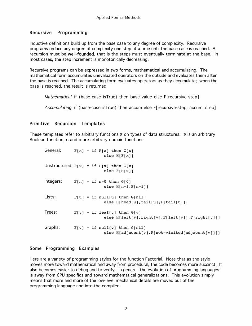
Applied Formal Methods
2
Recursive Programming
Inductive definitions build up from the base case to any degree of complexity. Recursive
programs reduce any degree of complexity one step at a time until the base case is reached. A
recursion must be wwell-founded, that is the steps must eventually terminate at the base. In
most cases, the step increment is monotonically decreasing.
Recursive programs can be expressed in two forms, mathematical and accumulating. The
mathematical form accumulates unevaluated operators on the outside and evaluates them after
the base is reached. The accumulating form evaluates operators as they accumulate; when the
base is reached, the result is returned.
Mathematical: if (base-case isTrue) then base-value else F[recursive-step]
Accumulating: if (base-case isTrue) then accum else F[recursive-step, accum+step]
Primitive Recursion Templates
These templates refer to arbitrary functions F on types of data structures. P is an arbitrary
Boolean function, G and H are arbitrary domain functions
General: F[x] = if P[x] then G[x]else H[F[x]]
Unstructured: F[x] = if P[x] then G[x]else F[H[x]]
Integers: F[n] = if n=0 then G[0]else H[n-1,F[n-1]]
Lists: F[u] = if null[u] then G[nil]else H[head[u],tail[u],F[tail[u]]]
Trees: F[v] = if leaf[v] then G[v]else H[left[v],right[v],F[left[v]],F[right[v]]]
Graphs: F[v] = if null[v] then G[nil]else H[adjacent[v],F[not-visited[adjacent[v]]]]
Some Programming Examples
Here are a variety of programming styles for the function Factorial. Note that as the style
moves more toward mathematical and away from procedural, the code becomes more succinct. It
also becomes easier to debug and to verify. In general, the evolution of programming languages
is away from CPU specifics and toward mathematical generalizations. This evolution simply
means that more and more of the low-level mechanical details are moved out of the
programming language and into the compiler.
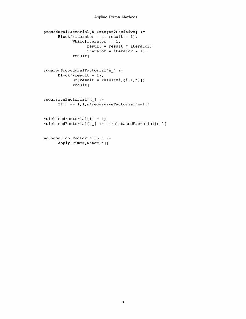
Applied Formal Methods
3
proceduralFactorial[n_Integer?Positive] :=Block[{iterator = n, result = 1}, While[iterator != 1,
result = result * iterator; iterator = iterator - 1];
result]
sugaredProceduralFactorial[n_] :=Block[{result = 1}, Do[result = result*i,{i,1,n}];
result]
recursiveFactorial[n_] :=If[n == 1,1,n*recursiveFactorial[n-1]]
rulebasedFactorial[1] = 1;rulebasedFactorial[n_] := n*rulebasedFactorial[n-1]
mathematicalFactorial[n_] :=Apply[Times,Range[n]]
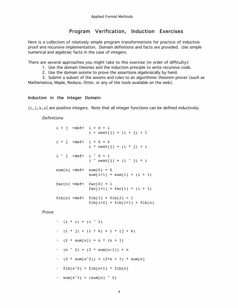
Applied Formal Methods
4
Program Verification, Induction Exercises
Here is a collection of relatively simple program transformations for practice of inductive
proof and recursive implementation. Domain definitions and facts are provided. Use simple
numerical and algebraic facts in the case of integers.
There are several approaches you might take to this exercise (in order of difficulty):
1. Use the domain theories and the induction principle to write recursive code.
2. Use the domain axioms to prove the assertions algebraically by hand.
3. Submit a subset of the axioms and rules to an algorithmic theorem prover (such as
Mathematica, Maple, Reduce, Otter, or any of the tools available on the web).
Induction in the Integer Domain:
{i,j,k,n} are positive integers. Note that all integer functions can be defined inductively.
Definitions
i + j =def= i + 0 = i i + next[j] = (i + j) + 1
i * j =def= i * 0 = 0 i * next[j] = (i * j) + i
i ^ j =def= i ^ 0 = 1 i ^ next[j] = (i ^ j) * i
sum[n] =def= sum[0] = 0 sum[i+1] = sum[i] + (i + 1)
fac[n] =def= fac[0] = 1 fac[i+1] = fac[i] * (i + 1)
fib[n] =def= fib[1] = fib[2] = 1 fib[i+2] = fib[i+1] + fib[n]
Prove
• (i * i) = (i ^ 2)
• (i * j) + (i * k) = i * (j + k)
• (2 * sum[n]) = n * (n + 1)
• (n ^ 2) = (2 * sum[n-1]) + n
• (3 * sum[n^2]) = (2*n + 1) * sum[n]
• fib[n^2] = fib[n+1] * fib[n]
• sum[n^3] = (sum[n] ^ 2)
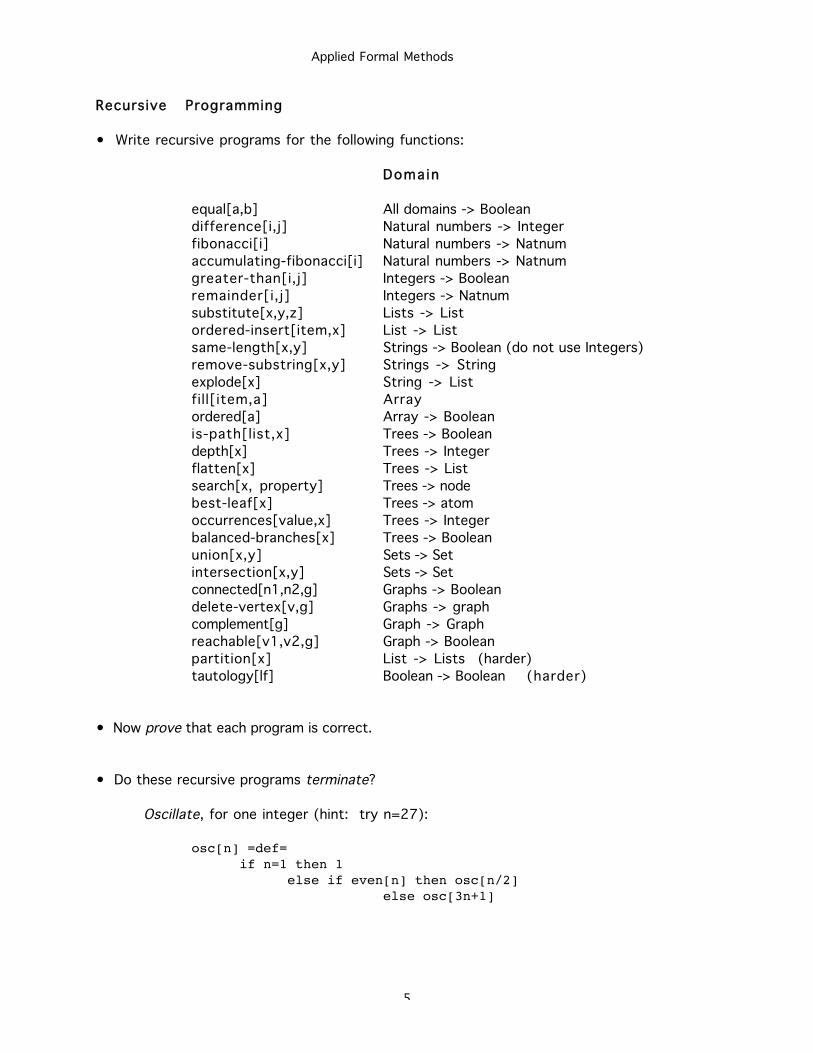
Applied Formal Methods
5
Recursive Programming
• Write recursive programs for the following functions:
Domain
equal[a,b] All domains -> Boolean
difference[i,j] Natural numbers -> Integer
fibonacci[i] Natural numbers -> Natnum
accumulating-fibonacci[i] Natural numbers -> Natnum
greater-than[i,j] Integers -> Boolean
remainder[i,j] Integers -> Natnum
substitute[x,y,z] Lists -> List
ordered-insert[item,x] List -> List
same-length[x,y] Strings -> Boolean (do not use Integers)
remove-substring[x,y] Strings -> String
explode[x] String -> List
fill[item,a] Array
ordered[a] Array -> Boolean
is-path[list,x] Trees -> Boolean
depth[x] Trees -> Integer
flatten[x] Trees -> List
search[x, property] Trees -> node
best-leaf[x] Trees -> atom
occurrences[value,x] Trees -> Integer
balanced-branches[x] Trees -> Boolean
union[x,y] Sets -> Set
intersection[x,y] Sets -> Set
connected[n1,n2,g] Graphs -> Boolean
delete-vertex[v,g] Graphs -> graph
complement[g] Graph -> Graph
reachable[v1,v2,g] Graph -> Boolean
partition[x] List -> Lists (harder)
tautology[lf] Boolean -> Boolean (harder)
• Now prove that each program is correct.
• Do these recursive programs terminate?
Oscillate, for one integer (hint: try n=27):
osc[n] =def=if n=1 then 1
else if even[n] then osc[n/2]else osc[3n+1]
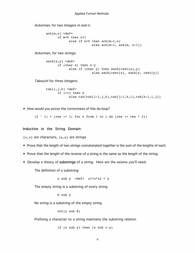
Applied Formal Methods
6
Ackerman, for two integers m and n:
ack[m,n] =def=if m=0 then n+1
else if n=0 then ack[m-1,n]else ack[m-1, ack[m, n-1]]
Ackerman, for two strings:
sack[x,y] =def=if (char x) then x•y
else if (char y) then sack[rest[x],y]else sack[rest[x], sack[x, rest[y]]
Takeuchi for three integers:
tak[i,j,k] =def=if i<=j then k
else tak[tak[i-1,j,k],tak[j-1,k,i],tak[k-1,i,j]]
• How would you prove the correctness of this do-loop?
(2 ^ i) = (res := 1; for n from 1 to i do (res := res * 2))
Induction in the String Domain:
{u,v} are characters, {x,y} are strings
• Prove that the length of two strings concatenated together is the sum of the lengths of each.
• Prove that the length of the reverse of a string is the same as the length of the string.
• Develop a theory of ssubstrings of a string. Here are the axioms you'll need:
The definition of a substring:
x sub y =def= z1*x*z2 = y
The empty string is a substring of every string
E sub y
No string is a substring of the empty string
not(y sub E)
Prefixing a character to a string maintains the substring relation
if (x sub y) then (x sub u•y)
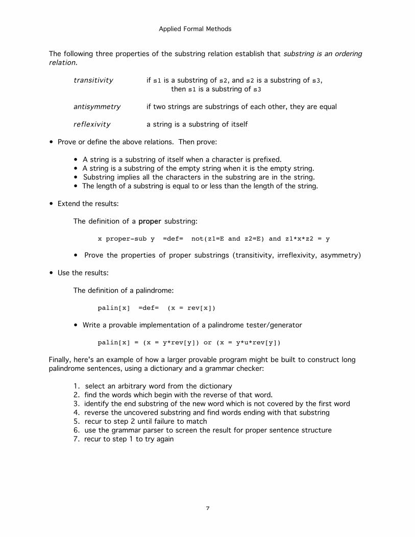
Applied Formal Methods
7
The following three properties of the substring relation establish that substring is an orderingrelation.
transitivity if s1 is a substring of s2, and s2 is a substring of s3,
then s1 is a substring of s3
antisymmetry if two strings are substrings of each other, they are equal
reflexivity a string is a substring of itself
• Prove or define the above relations. Then prove:
• A string is a substring of itself when a character is prefixed.
• A string is a substring of the empty string when it is the empty string.
• Substring implies all the characters in the substring are in the string.
• The length of a substring is equal to or less than the length of the string.
• Extend the results:
The definition of a pproper substring:
x proper-sub y =def= not(z1=E and z2=E) and z1*x*z2 = y
• Prove the properties of proper substrings (transitivity, irreflexivity, asymmetry)
• Use the results:
The definition of a palindrome:
palin[x] =def= (x = rev[x])
• Write a provable implementation of a palindrome tester/generator
palin[x] = (x = y*rev[y]) or (x = y*u*rev[y])
Finally, here's an example of how a larger provable program might be built to construct long
palindrome sentences, using a dictionary and a grammar checker:
1. select an arbitrary word from the dictionary
2. find the words which begin with the reverse of that word.
3. identify the end substring of the new word which is not covered by the first word
4. reverse the uncovered substring and find words ending with that substring
5. recur to step 2 until failure to match
6. use the grammar parser to screen the result for proper sentence structure
7. recur to step 1 to try again
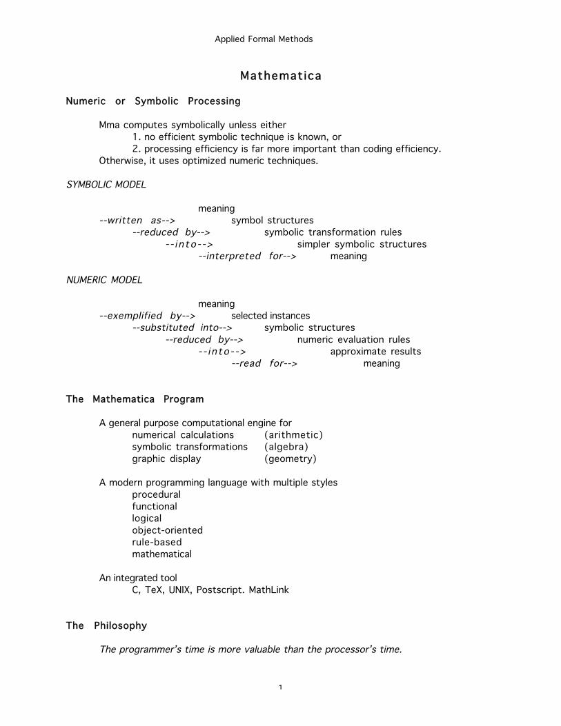
Applied Formal Methods
1
Mathematica
Numeric or Symbolic Processing
Mma computes symbolically unless either
1. no efficient symbolic technique is known, or
2. processing efficiency is far more important than coding efficiency.
Otherwise, it uses optimized numeric techniques.
SYMBOLIC MODEL
meaning
--written as--> symbol structures
--reduced by--> symbolic transformation rules
- - i n to - -> simpler symbolic structures
--interpreted for--> meaning
NUMERIC MODEL
meaning
--exemplified by--> selected instances
--substituted into--> symbolic structures
--reduced by--> numeric evaluation rules
- - i n to - -> approximate results
--read for--> meaning
The Mathematica Program
A general purpose computational engine for
numerical calculations (arithmetic)
symbolic transformations (algebra)
graphic display (geometry)
A modern programming language with multiple styles
procedural
functional
logical
object-oriented
rule-based
mathematical
An integrated tool
C, TeX, UNIX, Postscript. MathLink
The Philosophy
The programmer’s time is more valuable than the processor’s time.
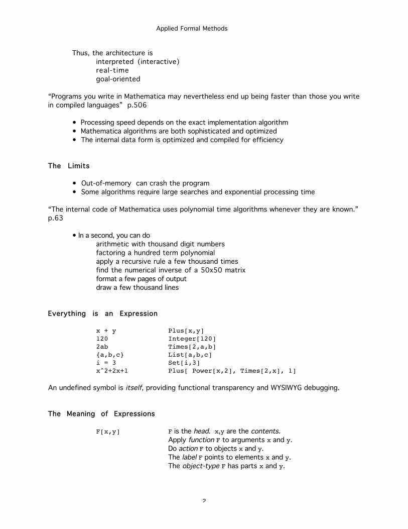
Applied Formal Methods
2
Thus, the architecture is
interpreted (interactive)
real-time
goal-oriented
“Programs you write in Mathematica may nevertheless end up being faster than those you write
in compiled languages” p.506
• Processing speed depends on the exact implementation algorithm
• Mathematica algorithms are both sophisticated and optimized
• The internal data form is optimized and compiled for efficiency
The Limits
• Out-of-memory can crash the program
• Some algorithms require large searches and exponential processing time
“The internal code of Mathematica uses polynomial time algorithms whenever they are known.”
p.63
• In a second, you can do
arithmetic with thousand digit numbers
factoring a hundred term polynomial
apply a recursive rule a few thousand times
find the numerical inverse of a 50x50 matrix
format a few pages of output
draw a few thousand lines
Everything is an Expression
x + y Plus[x,y]120 Integer[120]2ab Times[2,a,b]{a,b,c} List[a,b,c]i = 3 Set[i,3]x^2+2x+1 Plus[ Power[x,2], Times[2,x], 1]
An undefined symbol is itself, providing functional transparency and WYSIWYG debugging.
The Meaning of Expressions
F[x,y] F is the head. x,y are the contents.Apply function F to arguments x and y.
Do action F to objects x and y.
The label F points to elements x and y.
The object-type F has parts x and y.

Applied Formal Methods
3
The head can both act on its contents (as a function) and maintain the structure of its contents
(as an object), depending on context (the location of the expression, the presence of a
definition).
L i s t s
The boundary labeled List maintains its internal structure as a database.
Lists are used for all collections:
data record {John, 555-1234, [email protected]}vector {x, y, z}matrix { {11,12},{21,22} }set Union[{a,b},{a,c}] ==> {a,b,c}graphics spec Line[ {{0,1}, {1,1}, {1,0}} ]stream {1,2,3, ...}structure template {_, {_,_}, { {_,_},...} }
The Fundamental Principle of Computation
Take any expression and apply transformation rules until the result no longer changes.
1. Reduce head
2. Reduce each element base case arithmetic
3. Standardize
4. Apply user defined rules inductive case algebra
5. Apply built-in rules.
6. Reduce the result. recursion
The Internal Mechanism
All expressions are stored in an augmented binary transform table (?)
we see internal table entry
x=3 11001... 11a[1]=x 1000[1] 10110f[n_]=n^2 1011[#] 10110[#1110]
• The input expression is matched (using a linear-time algorithm) to the internal
table:E = 00110[0100011]001010[11101]
• Each match generates a substitution.
• No match causes no change.
• The structure of the expression is not a string but a network.
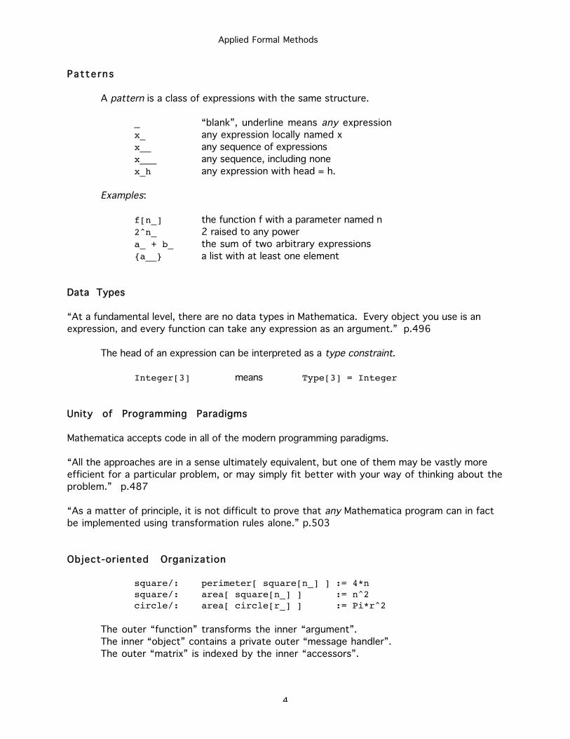
Applied Formal Methods
4
Patterns
A pattern is a class of expressions with the same structure.
_ “blank”, underline means any expression
x_ any expression locally named x
x__ any sequence of expressions
x___ any sequence, including none
x_h any expression with head = h.
Examples:
f[n_] the function f with a parameter named n
2^n_ 2 raised to any power
a_ + b_ the sum of two arbitrary expressions
{a__} a list with at least one element
Data Types
“At a fundamental level, there are no data types in Mathematica. Every object you use is an
expression, and every function can take any expression as an argument.” p.496
The head of an expression can be interpreted as a type constraint.
Integer[3] means Type[3] = Integer
Unity of Programming Paradigms
Mathematica accepts code in all of the modern programming paradigms.
“All the approaches are in a sense ultimately equivalent, but one of them may be vastly more
efficient for a particular problem, or may simply fit better with your way of thinking about the
problem.” p.487
“As a matter of principle, it is not difficult to prove that any Mathematica program can in fact
be implemented using transformation rules alone.” p.503
Object-oriented Organization
square/: perimeter[ square[n_] ] := 4*nsquare/: area[ square[n_] ] := n^2circle/: area[ circle[r_] ] := Pi*r^2
The outer “function” transforms the inner “argument”.
The inner “object” contains a private outer “message handler”.
The outer “matrix” is indexed by the inner “accessors”.
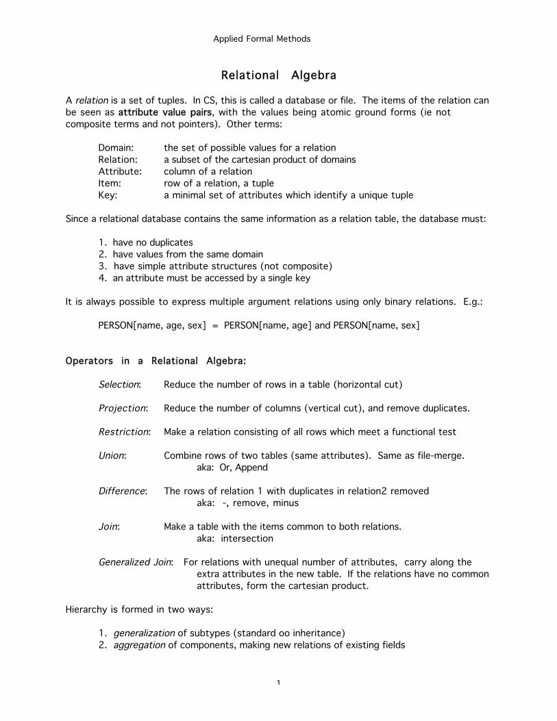
Applied Formal Methods
1
Relational Algebra
A relation is a set of tuples. In CS, this is called a database or file. The items of the relation can
be seen as aattribute value pairs, with the values being atomic ground forms (ie not
composite terms and not pointers). Other terms:
Domain: the set of possible values for a relation
Relation: a subset of the cartesian product of domains
Attribute: column of a relation
Item: row of a relation, a tuple
Key: a minimal set of attributes which identify a unique tuple
Since a relational database contains the same information as a relation table, the database must:
1. have no duplicates
2. have values from the same domain
3. have simple attribute structures (not composite)
4. an attribute must be accessed by a single key
It is always possible to express multiple argument relations using only binary relations. E.g.:
PERSON[name, age, sex] = PERSON[name, age] and PERSON[name, sex]
Operators in a Relational Algebra:
Selection: Reduce the number of rows in a table (horizontal cut)
Projection: Reduce the number of columns (vertical cut), and remove duplicates.
Restriction: Make a relation consisting of all rows which meet a functional test
Union: Combine rows of two tables (same attributes). Same as file-merge.
aka: Or, Append
Difference: The rows of relation 1 with duplicates in relation2 removed
aka: -, remove, minus
Join: Make a table with the items common to both relations.
aka: intersection
Generalized Join: For relations with unequal number of attributes, carry along the
extra attributes in the new table. If the relations have no common
attributes, form the cartesian product.
Hierarchy is formed in two ways:
1. generalization of subtypes (standard oo inheritance)
2. aggregation of components, making new relations of existing fields
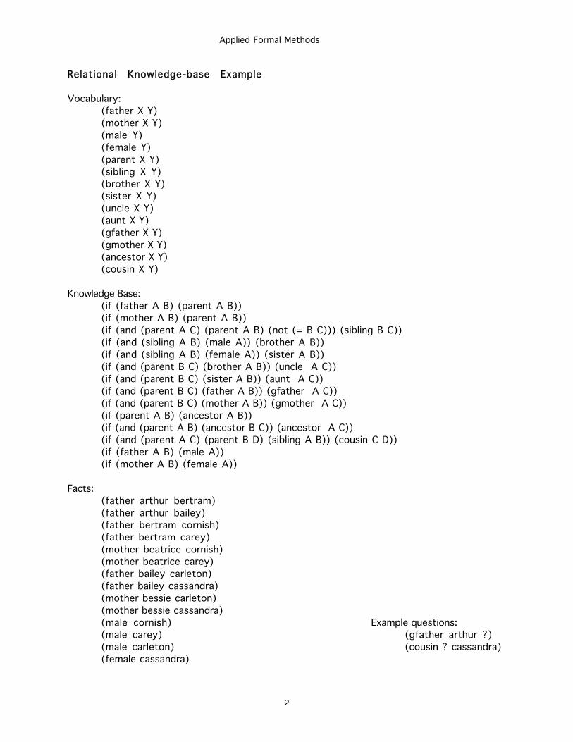
Applied Formal Methods
2
Relational Knowledge-base Example
Vocabulary:
(father X Y)
(mother X Y)
(male Y)
(female Y)
(parent X Y)
(sibling X Y)
(brother X Y)
(sister X Y)
(uncle X Y)
(aunt X Y)
(gfather X Y)
(gmother X Y)
(ancestor X Y)
(cousin X Y)
Knowledge Base:
(if (father A B) (parent A B))
(if (mother A B) (parent A B))
(if (and (parent A C) (parent A B) (not (= B C))) (sibling B C))
(if (and (sibling A B) (male A)) (brother A B))
(if (and (sibling A B) (female A)) (sister A B))
(if (and (parent B C) (brother A B)) (uncle A C))
(if (and (parent B C) (sister A B)) (aunt A C))
(if (and (parent B C) (father A B)) (gfather A C))
(if (and (parent B C) (mother A B)) (gmother A C))
(if (parent A B) (ancestor A B))
(if (and (parent A B) (ancestor B C)) (ancestor A C))
(if (and (parent A C) (parent B D) (sibling A B)) (cousin C D))
(if (father A B) (male A))
(if (mother A B) (female A))
Facts:
(father arthur bertram)
(father arthur bailey)
(father bertram cornish)
(father bertram carey)
(mother beatrice cornish)
(mother beatrice carey)
(father bailey carleton)
(father bailey cassandra)
(mother bessie carleton)
(mother bessie cassandra)
(male cornish) Example questions:
(male carey) (gfather arthur ?)
(male carleton) (cousin ? cassandra)
(female cassandra)
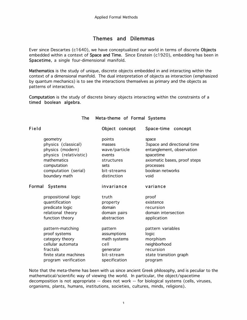
Applied Formal Methods
1
Themes and Dilemmas
Ever since Descartes (c1640), we have conceptualized our world in terms of discrete OObjects
embedded within a context of SSpace and Time. Since Einstein (c1920), embedding has been in
Spacetime, a single four-dimensional manifold.
Mathematics is the study of unique, discrete objects embedded in and interacting within the
context of a dimensional manifold. The dual interpretation of objects as interaction (emphasized
by quantum mechanics) is to see the interactions themselves as primary and the objects as
patterns of interaction.
Computation is the study of discrete binary objects interacting within the constraints of a
timed boolean algebra.
The Meta-theme of Formal Systems
F i e l d Object concept Space-time concept
geometry points space
physics (classical) masses 3space and directional time
physics (modern) wave/particle entanglement, observation
physics (relativistic) events spacetime
mathematics structures axiomatic bases, proof steps
computation sets processes
computation (serial) bit-streams boolean networks
boundary math distinction void
Formal Systems i nva r i ance va r i ance
propositional logic truth proof
quantification property existence
predicate logic domain recursion
relational theory domain pairs domain intersection
function theory abstraction application
pattern-matching pattern pattern variables
proof systems assumptions logic
category theory math systems morphism
cellular automata cell neighborhood
fractals generator recursion
finite state machines bit-stream state transition graph
program verification specification program
Note that the meta-theme has been with us since ancient Greek philosophy, and is peculiar to the
mathematical/scientific way of viewing the world. In particular, the object/spacetime
decomposition is not appropriate -- does not work -- for biological systems (cells, viruses,
organisms, plants, humans, institutions, societies, cultures, minds, religions).
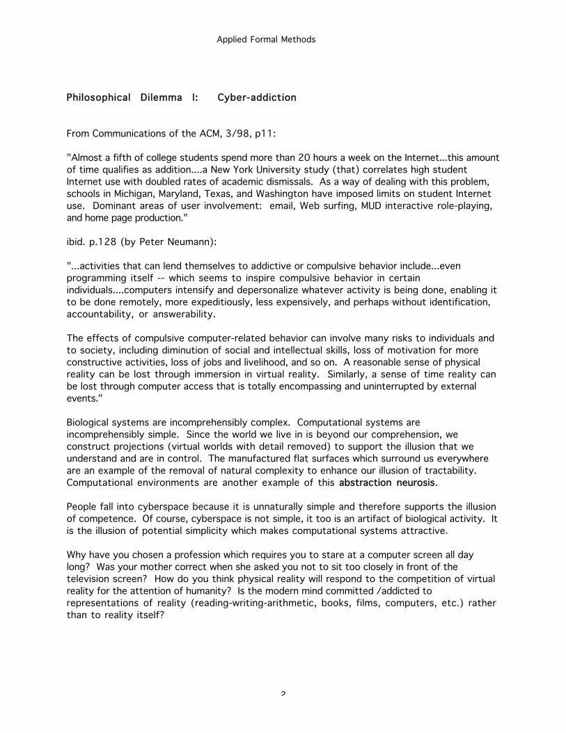
Applied Formal Methods
2
Philosophical Dilemma I: Cyber-addiction
From Communications of the ACM, 3/98, p11:
"Almost a fifth of college students spend more than 20 hours a week on the Internet...this amount
of time qualifies as addition....a New York University study (that) correlates high student
Internet use with doubled rates of academic dismissals. As a way of dealing with this problem,
schools in Michigan, Maryland, Texas, and Washington have imposed limits on student Internet
use. Dominant areas of user involvement: email, Web surfing, MUD interactive role-playing,
and home page production."
ibid. p.128 (by Peter Neumann):
"...activities that can lend themselves to addictive or compulsive behavior include...even
programming itself -- which seems to inspire compulsive behavior in certain
individuals....computers intensify and depersonalize whatever activity is being done, enabling it
to be done remotely, more expeditiously, less expensively, and perhaps without identification,
accountability, or answerability.
The effects of compulsive computer-related behavior can involve many risks to individuals and
to society, including diminution of social and intellectual skills, loss of motivation for more
constructive activities, loss of jobs and livelihood, and so on. A reasonable sense of physical
reality can be lost through immersion in virtual reality. Similarly, a sense of time reality can
be lost through computer access that is totally encompassing and uninterrupted by external
events."
Biological systems are incomprehensibly complex. Computational systems are
incomprehensibly simple. Since the world we live in is beyond our comprehension, we
construct projections (virtual worlds with detail removed) to support the illusion that we
understand and are in control. The manufactured flat surfaces which surround us everywhere
are an example of the removal of natural complexity to enhance our illusion of tractability.
Computational environments are another example of this aabstraction neurosis.
People fall into cyberspace because it is unnaturally simple and therefore supports the illusion
of competence. Of course, cyberspace is not simple, it too is an artifact of biological activity. It
is the illusion of potential simplicity which makes computational systems attractive.
Why have you chosen a profession which requires you to stare at a computer screen all day
long? Was your mother correct when she asked you not to sit too closely in front of the
television screen? How do you think physical reality will respond to the competition of virtual
reality for the attention of humanity? Is the modern mind committed /addicted to
representations of reality (reading-writing-arithmetic, books, films, computers, etc.) rather
than to reality itself?
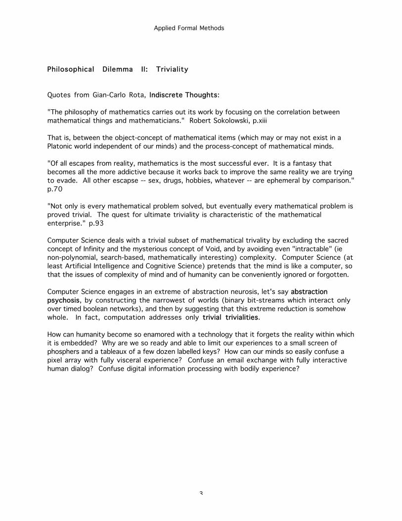
Applied Formal Methods
3
Philosophical Dilemma II: Triviality
Quotes from Gian-Carlo Rota, IIndiscrete TThoughts:
"The philosophy of mathematics carries out its work by focusing on the correlation between
mathematical things and mathematicians." Robert Sokolowski, p.xiii
That is, between the object-concept of mathematical items (which may or may not exist in a
Platonic world independent of our minds) and the process-concept of mathematical minds.
"Of all escapes from reality, mathematics is the most successful ever. It is a fantasy that
becomes all the more addictive because it works back to improve the same reality we are trying
to evade. All other escapse -- sex, drugs, hobbies, whatever -- are ephemeral by comparison."
p.70
"Not only is every mathematical problem solved, but eventually every mathematical problem is
proved trivial. The quest for ultimate triviality is characteristic of the mathematical
enterprise." p.93
Computer Science deals with a trivial subset of mathematical trivality by excluding the sacred
concept of Infinity and the mysterious concept of Void, and by avoiding even "intractable" (ie
non-polynomial, search-based, mathematically interesting) complexity. Computer Science (at
least Artificial Intelligence and Cognitive Science) pretends that the mind is like a computer, so
that the issues of complexity of mind and of humanity can be conveniently ignored or forgotten.
Computer Science engages in an extreme of abstraction neurosis, let's say aabstraction
psychosis, by constructing the narrowest of worlds (binary bit-streams which interact only
over timed boolean networks), and then by suggesting that this extreme reduction is somehow
whole. In fact, computation addresses only ttrivial trivialities.
How can humanity become so enamored with a technology that it forgets the reality within which
it is embedded? Why are we so ready and able to limit our experiences to a small screen of
phosphers and a tableaux of a few dozen labelled keys? How can our minds so easily confuse a
pixel array with fully visceral experience? Confuse an email exchange with fully interactive
human dialog? Confuse digital information processing with bodily experience?


![benjaminleewilliams.files.wordpress.com · Web view[Type text][Type text][Type text] Venue: Porthcawl Comprehensive 2013-2014 Course: Drawing Course code: PC002/J8/14-15](https://static.fdocuments.in/doc/165x107/6002da0b880468788c348ac4/web-view-type-texttype-texttype-text-venue-porthcawl-comprehensive-2013-2014.jpg)