Course 2: Water Quality and Pollution - un-ihe.org
36
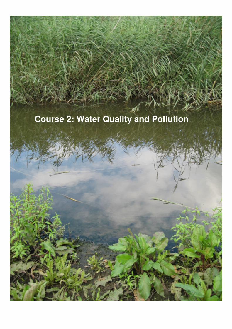
Course 2: Water Quality and Pollution
Transcript of Course 2: Water Quality and Pollution - un-ihe.org
Course 2: Water Quality and Pollution

UNESCO-IHE Institute for Water Education Course 2 OLC Water Quality Assessment Page 2
Course 2: Water Quality and Pollution Table of Contents
Unit 1 Introduction to Water Quality and Pollution
Unit 2 Organic matter
Unit 3 Nutrients
Unit 4 Micropollutants
Unit 5 Aquatic ecosystems
Unit 6
Water quality modelling (optional)

UNESCO-IHE Institute for Water Education Course 2 OLC Water Quality Assessment Page 3
Unit 1 – Introduction to Water Quality and Pollution
1.1. Water uses and functions
In this unit we will give a short overview of:
1. Water uses and functions, and especially the water quality demands related to
various uses;
2. Translation of water quality demands into water quality standards;
3. Natural water quality, or in other the background concentrations of certain
substances that occur in rivers and lake even without human interference;
4. Sources of pollution, also in relation to environmental compartments;
5. Spatial and temporal variations of water quality and pollution.
We have earlier defined pollution as “the introduction by man, directly or indirectly, of
substances or energy which result in deleterious effects" such as: (1) harm to living
resources/aquatic ecosystems; (2) hazards to human health; (3) hindrance to aquatic
activities including fishing, boating, energy production; (4) impairment of water quality
with respect to its use in agricultural, industrial and often economic activities; and (5)
reduction of amenities.
From this definition of pollution, we can easily derive a definition for water quality:
“Water quality expresses the suitability of water for various uses or processes: drinking
water; irrigation water; nature conservation, etc”. A more complete list of uses was
given in Unit 4 of Course 1.
Thus, based on its intended use, we can define different water quality requirements:
− No or hardly any specific requirements: typical examples are navigation water or
power generation
− Defined “minimum standards”: typical examples are irrigation water, fisheries,
recreation water
− “Undisturbed quality”: needed for good ecosystem functioning.
1.2. Water quality standards
Water quality requirements are usually specified as water quality standards (WQS). In
the past WQS mostly consisted of physicochemical requirements such as pH levels,
nitrogen concentrations etc. In the past 10-15 year however, there has been an
evolution to interpret water quality more holistically by not only looking at the chemistry,
but also at the biology and ecology: which algae are present; which fish are present
etc?
We can illustrate this idea with a very simple example: many fish species require
specific habitat conditions for spawning (plants to attach the eggs to, or muddy
sediment to bury the eggs into). Many rivers however have been channelized in the
past, and instead of having natural banks they are now contained within a pair of
concrete walls. Even though the physico-chemical water quality can be excellent in

UNESCO-IHE Institute for Water Education Course 2 OLC Water Quality Assessment Page 4
these rivers, fishes will be absent because of the lack of plants needed for
reproduction.
A similar example is the story of the salmon. This is a so-called anadromous fish,
meaning that it lives part of its life in the sea, but that it migrates upstream into
freshwater for spawning. Because of severe water pollution in the 1960s and 1970s,
salmon disappeared from many European rivers. However, now that many wastewater
treatment plants have been put into operation and that the river water quality has
improved a lot, the population of salmon is not recovering as well as you would expect.
This can be attributed to the multitude of “fish migration barriers” such as dams,
sluices, weirs, etc., which form, in many cases, an impenetrable barrier for the fish
(www.eaa-europe.eu/fileadmin/templates/uploads/Positions/Salmon_and_Migration_Barriers-
final.pdf). The fact that salmon is absent in a certain river can thus point not only to
chemical pollution, but also to structural problems.
To come back to water quality: looking only at the chemical water quality is not
sufficient to tell you whether or not a river is “healthy”; one should also look at the biota.
This idea is the key concept of the recent European Water Framework Directive
(Directive 2000/60/EC), (EUWFD), which demands that all water bodies within the EU
must have reached, in 2015, a good ecological status. Specific monitoring instructions
are given not only with regards to the physical and chemical parameters to be
monitored, but also with respect to the biological parameters (fish, plants, plankton, ...).
Ecological monitoring and monitoring in the EUWFD will further be discussed in Course
3; for now we will focus on physico-chemical standards because many countries all
over the world still solely make use of this type of WQS. On pages 92-94 of the book of
Chapman (1996), you can find a general overview of WQS applied in different parts of
the world, and according to different water uses.
Note that in many cases, there are not only specifications about the desired or
maximum concentration, but also requirements on the number of samples to be taken
each year (sampling frequency), the number of samples that should fulfil the standard
(all samples or 90% of the samples or ...); in specific cases also a difference can be
made between average values and absolute values. In Flanders (Belgium) for instance,
the average concentration of NH4-N in a river (average of one year’s worth of data)
should be less than 1 mg N/L, but every single sample has to meet the absolute
standard of 5 mg N/L.
The water quality standards may be quite different for above different water uses.
Irrigation water, for example, hardly has requirements for dissolved oxygen and
nutrients. On the other hand, there will be specific requirements for chloride, boron etc,
in view of reduced crop yields at elevated concentrations. For recreation water, the
standards are especially related with aesthetic quality (colour, algae) and bacterial
pollution (expressed with the indicator E-coli).
Water fit for ecosystems need virtually undisturbed water quality; much emphasis is
given to the micropollutants levels (heavy metals, pesticides, PCBs, etc.). Industries
should use “Best Available Technologies” (BAT) to minimise waste loads, or even
apply zero discharges. For the other water uses, often the “ALARA principle” is
applied: “As low as reasonably achievable”.
UNESCO-IHE Institute for Water Education Course 2 OLC Water Quality Assessment Page 5
Assignment WQA-3: Water quality standards of your own country or region
Please look up the water quality standards of your country or region. Select maximally
20 parameters and report on their standards for different uses. If available, also specify
sampling frequencies etc. Submit your assignment as a table in Word or Excel via the
WQA-3 Forum on the site (as you have done before with the GEMS data).
1.3. Natural water quality
It is important to realise that even without any human interference, there is no "distilled
water" flowing through a river. There will always be non-zero “background”
concentrations of many substances, resulting from natural processes. For instance,
eruption of volcanoes can bring huge amounts of pollutants into the water. Another
example is mountain rivers which are continuously eroding the rocks over which they
flow, and as such carry some of the eroded materials with them; see PowerPoint 2.1. of
this Course.
Natural water quality varies from place to place, with the seasons, with climate, and
with the types of soils and rocks through which water moves. When water from rain or
snow moves over the land and through the ground, the water may dissolve minerals in
rocks and soil, percolate through organic material such as roots and leaves, and react
with algae, bacteria and other microscopic organisms. Water may also carry plant
debris and sand, silt, and clay to rivers and streams making the water appear “muddy”
or turbid. When water evaporates from lakes and streams, dissolved minerals are more
concentrated in the water that remains. Each of these natural processes changes the
water quality and potentially the water use.
The most common dissolved substances in water are minerals or salts that, as a group,
are referred to as dissolved solids. Dissolved solids include common constituents such
as calcium, sodium, bicarbonate and chloride; plant nutrients such as nitrogen and
phosphorus; and trace elements such as selenium, chromium, and arsenic. Also
dissolved gases such as oxygen and radon are common in natural waters.
A good further overview is given in Chapman (1996). Please read sections 6.3.1 and
6.3.2 on pages 256-263.
1.4. Sources of pollution
Taking into account the concept of natural water quality, we can also expand our
definition of pollution, as follows: “pollution is any deviation from the natural water
quality caused by human interference”.
Man can in many ways cause pollution of the aquatic environment; an overview is
given in Table 1 (taken from the book of Chapman) and details of the sources of each
pollutant will be given in the subsequent units. For now, it is important to realise that
pollution not only comes from the classical sewer pipes discharging into rivers and

UNESCO-IHE Institute for Water Education Course 2 OLC Water Quality Assessment Page 6
lakes (“point sources”), but also from urban and agricultural runoff (“non-point or diffuse
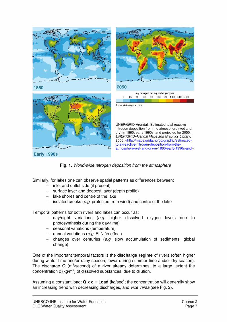
sources” and “mixed sources”) and even from the atmosphere. As an illustration of the
latter, Fig. 1 from the Millennium Ecosystem Assessment is given below, which shows
the evolution of worldwide nitrogen deposition (past, present and projected future).
Atmospheric deposition currently accounts for roughly 12% of the reactive nitrogen
entering terrestrial and coastal marine ecosystems globally, although in some regions,
atmospheric deposition accounts for a higher percentage (about 33% in the USA).
TABLE 1
1.5. Spatial and temporal variations
The water quality of a river or lake is not is difficult to represent in a single value, not
only because of the range of pollution sources and polluting compounds, but also
because there are important variations both in space and in time.
Typical spatial patterns or differences in rivers occur between:
− source and mouth (length profile)
− surface layer and deepest layer (depth profile)
− river banks and centre of the stream (width profile)
UNESCO-IHE Institute for Water Education Course 2 OLC Water Quality Assessment Page 7
UNEP/GRID-Arendal, 'Estimated total reactive nitrogen deposition from the atmosphere (wet and dry) in 1860, early 1990s, and projected for 2050', UNEP/GRID-Arendal Maps and Graphics Library, 2005, <http://maps.grida.no/go/graphic/estimated-total-reactive-nitrogen-deposition-from-the-atmosphere-wet-and-dry-in-1860-early-1990s-and>
Fig. 1. World-wide nitrogen deposition from the atmosphere
Similarly, for lakes one can observe spatial patterns as differences between:
− inlet and outlet side (if present)
− surface layer and deepest layer (depth profile)
− lake shores and centre of the lake
− isolated creeks (e.g. protected from wind) and centre of the lake
Temporal patterns for both rivers and lakes can occur as:
− day/night variations (e.g. higher dissolved oxygen levels due to
photosynthesis during the day-time)
− seasonal variations (temperature)
− annual variations (e.g. El Niño effect)
− changes over centuries (e.g. slow accumulation of sediments, global
change)
One of the important temporal factors is the discharge regime of rivers (often higher
during winter time and/or rainy season; lower during summer time and/or dry season).
The discharge Q (m3/second) of a river already determines, to a large, extent the
concentration c (kg/m3) of dissolved substances, due to dilution.
Assuming a constant load: Q x c = Load (kg/sec); the concentration will generally show
an increasing trend with decreasing discharges, and vice versa (see Fig. 2).

UNESCO-IHE Institute for Water Education Course 2 OLC Water Quality Assessment Page 8
In contrast, the total suspended solids (TSS) in a river often show an increasing trend
with higher discharges (see Fig. 3). This can be ascribed to the largely increased
erosion rates connected to rain storm events. Short-term peaks in TSS are often
missed because of the short duration of these rain storms.
From the above overview, we can already make a nice link to Course 3 – "Water
quality Monitoring", because some of the challenges of monitoring are not only the
“What?” questions (Which pollutants?) but also the “Where?” and “When?”. For now
however, we will remain with the “What?” question and discuss the various groups of
pollutants in the next units.
Action List for Unit 1 • Look and listen to the PowerPoint presentation available under “Lecture”. • Complete the assignment WQA-3 and put on the platform.
Assignment WQA-3: Water quality standards of your own country or region
Look up the water quality standards of your country or region. Select maximum 20
parameters and report on their standards for different uses. If available, also specify
sampling frequencies etc. Present your assignment as a table in Word or Excel.
Fig. 2
Fig. 3

UNESCO-IHE Institute for Water Education Course 2 OLC Water Quality Assessment Page 9
Unit 2 – Organic Matter
2.1. Forms of organic matter (OM)
There are millions of different organic compounds. This means it is almost impossible
to analyse all of them (technical and financial limitations). Therefore, very often
“lumped” parameters are used, which analyse a part of or all organic components at
once. Common lumped parameters are:
− BOD: Biochemical Oxygen Demand
− COD: Chemical Oxygen Demand
− TOC: Total Organic Carbon
− (N)OM: (Natural) Organic Matter
BOD and COD are both based on the concept of oxygen demand, which starts from
the assumption that OM can be oxidized by oxygen into simple components such as
CO2 and H2O. The difference between both is that for BOD the reaction uses the
"natural" bacteria, whereas for COD it is a purely chemical reaction.
Theoretical oxygen demand, ThOD
The ThOD of a component can be derived from the stoichiometry of the oxidation
reaction. An example is given below, for ethanol, C2H5OH :
Oxidation reaction: C2H5OH + 3 O2 --> 2 CO2 + 3 H2O, so breahk-down of 1 mole of
ethanol requires 3 moles of oxygen. With molecular weights (M.W.) of C2H5OH: 46
g/mole; O2 : 32 g/mole) --> 46 g. C2H5OH requires 96 g. O2 .
So 1 g. ethanol requires 2.08 g. oxygen: ThOD (C2H5OH) = 2.08 mg O2 per mg ethanol.
Alternatively, knowing its concentration, the ThOD can also be expressed in mg/L. E.g.
for a wastewater with 100 mg/L ethanol, the ThOD will be: 208 mg/L.
Applying ThOD can only be done if you know exactly which components are present,
and at which concentrations. Also, not every compound can be completely oxidised;
some resist degradation and will have an actual oxygen demand which is (often much)
lower than the theoretical one. Therefore, in practice COD and BOD are used, rather
than ThOD.
Chemical Oxygen Demand, COD
COD is measured by oxidation of the samples in the laboratory, using strong chemical
oxidants (mostly K2Cr2O7) and strong acidic conditions (pH around 0) and boiling for 2
hours. Usually a "recovery" >95% is attained, meaning that more than 95% of the OM
is oxidised and thus accounted for. The advantage of COD is that the analysis takes
relatively little time: around 2.5 hours, and even less for a "rapid COD test". A
disadvantage of COD is that the parameter does not really mimic the actual
degradation processes in nature. For that the following parameter is more suitable.
Biochemical Oxygen Demand, BOD
BOD is measured by microbial decomposition in the laboratory under standardized
conditions (temperature, time): BOD205 i.e. BOD during 5 days at 20 ºC. This means
that only biodegradable OM will be taken into account. Since degradation may take

UNESCO-IHE Institute for Water Education Course 2 OLC Water Quality Assessment Page 10
even a month or more, the value is usually around 40% of the COD value and often (in
case of non-degradable materials in the water) much lower.
t is important to realise that during a BOD or COD test, not only carbon-related
compounds can be oxidized, but also e.g. ammonia.. This extra oxygen demand is thus
not representative for the amount of organic material (or organic carbon) in the water.
The most common, and also most important one, is the nBOD or Nitrogen Biochemical
Oxygen Demand, originating from the nitrification reaction:
NH4+ + 2 O2 --> NO3
- + 2 H+ + H2O , or:
1 mole of NH4-N requires 2 moles of O2, so 1 g. NH4-N requires 4.57 g O2 (footnote 1)
So the nBOD can give a large contribution to the total BOD! In estimating the cost of
wastewater treatment, for which "aeration" (oxygen supply) is the largest contributor,
this nBOD is certainly taken into account. To find out the cBOD term only, a
“nitrification inhibitor” can be added in the lab. In that case one uses the term cBOD or
carbon(aceous) BOD. Without nitrification inhibitor, the term tBOD or total BOD is used.
Organic matter mainly comes from domestic and industrial sources. Concentrations
can vary greatly (for example from 430 mg/L of COD in medium-strength domestic
wastewater up to 150,000 mg/L of COD in landfill leachates; the COD values thus
have to be examined on a case-by-case base.
In the Netherlands, the standards for acceptable surface water quality are set at:
BOD205 < 3.0 mg/L
COD < 20 mg/L
Common effluent standards (domestic wastewater after treatment) in Europe are:
BOD205 < 25 mg/L
COD < 125 mg/L
1 Note that in water quality monitoring, charges are often left out; similarly: mg PO4 /L, mg NO3 /L
INTERMEZZO: NH4-N or NH4?
In water quality monitoring we can express the concentration of the constituent:
• Based on the molecule, so as mg NH4/L (M.W. = 14 + 4 =18) (rounded off)
• Based on the atom(s), so as mg NH4-N/L (Atomic weight A.W. = 14) Thus a water quality of 1.0 mg NH4/L corresponds to 0.78 mg NH4- N/L . Similarly: the Worlds Health Organization, WHO, guideline for nitrate in drinking water = 50 mg NO3/L, equivalent to (14/62)*50 = 11.3 mg NO3-N/L .
It is highly recommendable to follow the "Atoms system", e.g. because only then,
mass balances and flows can be estimated.
Be very aware, in water quality data interpretation as well as in your own data
reporting, of the way the results are expressed!

UNESCO-IHE Institute for Water Education Course 2 OLC Water Quality Assessment Page 11
Total organic carbon
Total organic carbon (TOC) is the amount of carbon bound in an organic compound 2
and is often used as a non-specific indicator of water quality. It can further be
subdivided into dissolved and particulate components (DOC and POC).
Natural organic matter
Natural organic matter (NOM) is broken down organic matter that comes from plants
and animals in the environment. Examples are "humic acids" (see Chapman, p. 100).
10-35% of the carbon present forms aromatic rings; these rings are very stable due to
"resonance stabilization", so they are difficult to break down. The main concern of
having NOM in water is that it may react with chlorine and other disinfectants during
drinking water production, producing disinfection by-products, many of which are either
carcinogenic or mutagenic.
2.2. Impacts
Following a BOD discharge, the dissolved oxygen (DO) concentration in a river
typically shows a decrease due to the BOD degradation (oxygen demand), followed by
a recovery caused by the re-aeration from the atmosphere: “oxygen sag curve”; see
Fig.4.
Fig.4. Oxygen sag curve for low-high BOD inputs in a river
The oxygen minimum may be reached some 50 kilometres from the BOD discharge;
thus the effect of BOD discharges is often an interregional or even international
problem. The minimum DO can be found with the help of the following formula3:
2 "Organic compounds" entail all those with the atom C present, except CO2, Carbonates, CN
- , and a few
more 3 For details, see Unit 2.6.: Water quality Modelling

UNESCO-IHE Institute for Water Education Course 2 OLC Water Quality Assessment Page 12
In which:
− L0 = BOD concentration in the river directly downstream of the waste discharge,
after mixing (mg/L)
− cmin = O2 minimum (mg/L)
− cs = O2 saturation concentration (mg/L), usually around 10 mg/L, but lower for
higher water temperatures
− k1 = BOD decay rate constant (day-1); its value is usually 0.2-0.4 day-1
− k2 = re-aeration rate constant (day-1); its value lies usually between 0.2 and 2 day-1,
with high values for shallow, fast-flowing rivers
− tc = travel time of the river to reach the DO minimum (days)
The above formula shows that the “oxygen deficit” [cs – cmin] is roughly proportional to
the BOD load onto the river. This offers a way of solving BOD problems, by reducing
the BOD waste discharges. Be aware that at lower temperatures, more oxygen can
dissolve into the water and microbial degradation processes will be slower, so the
impact of wastewater discharge during winter is smaller than during summer.
See also examples of calculations in Unit 2.6.: "Water quality Modelling".
A nice illustration of these principles can be found at:
http://techalive.mtu.edu/meec/module02/WWTCost.html
Unit 3 – Nutrients
In this unit, we will discuss the influence of nutrients on the aquatic environment. We
will learn about their sources, their cycles and some of the consequences their
presence has on the water and the biota in it.
PART 1 - NITROGEN
3.1. Forms of N
There are four basic forms of nitrogen that can be found in aquatic environments -
nitrogen gas, organic nitrogen, ammonium and nitrate/nitrite. All forms of nitrogen
together are called total Nitrogen (TN) which can have concentrations between 0.4 µg/l
to several mg/l and is often measured to gain an insight into the nutrient status of the
waters (eutrophication status; we will hear more about this later on). Particulate
nitrogen is also distinguished from dissolved forms based on size (by filtration; see
Course 3.6.: dissolved nitrogen is < 0.45 microns). Particulate nitrogen is generally
organic nitrogen and is composed of detritus (e.g. leaf litter, animal faeces, etc.), and
other living algae, plants and animals.
ctk
s ek
Lkcc 1
2
01min
−
=−
UNESCO-IHE Institute for Water Education Course 2 OLC Water Quality Assessment Page 13
N2 gas makes up 78% of our atmosphere, is soluble in water but also biologically inert.
Only specialized organisms have developed the ability to use nitrogen gas directly and
use it as a nitrogen source through the process of biological nitrogen fixation (BNF).
Another component is made up by organic nitrogen compounds, which are largely
made up of amino acids, nucleotides and excretory products.
Further, ammonia (NH3; especially toxic for fish) is largely present in water as
ammonium (NH4+ ; hardly toxic), as a function of pH (see the PowerPoint
presentation 4 ) and is produced by the decomposition of organic matter, such as
proteins, by bacteria as well as a product of N fixation. It is also the preferred form of N
uptake for phytoplankton and plants. When oxygen is present, ammonium also easily
oxidizes to nitrate through the process of nitrification; we have just discussed this
reaction. Since ammonia is largely present in animal wastes, its introduction into water
ways easily leads to oxygen depletion in the water column. Lastly, Nitrate (NO3-) and
Nitrite (NO2-) are common forms of nitrogen found in water when oxygen is present.
Nitrate can be taken up by plants, algae and microbes.
3.2. Sources of Nitrogen (based on: http://www.ext.colostate.edu/pubs/crops/00550.html)
As mentioned before, the earth's atmosphere consists of 78% nitrogen and is the
ultimate source of nitrogen. In most areas of the world, the nitrogen found in soil
minerals is negligible. Manure contains an appreciable amount of nitrogen. Most of this
nitrogen is in organic forms: proteins and related compounds. Cattle manure contains
about 5 to 20 kg. of nitrogen per tonne. About half of this nitrogen is converted to forms
available to plants during the first growing season. Lower amounts are converted
during succeeding seasons. Commercial fertilizer nitrogen is effective when properly
applied. Fertilizer nitrogen is subject to the same transformations as other sources of
nitrogen. Both ammonium and nitrate enter the plant from commercial fertilizer, the
same way as that produced from natural products such as manure, crop residues or
organic fertilizers.
3.3. The Nitrogen Cycle
Different pathways of nitrogen transformation are described in Fig. 5. In the "complete"
N cycle, we distinguish point sources and non-point sources. Examples of the first
category are municipal and industrial wastewater; of the second: agricultural run-off.
The transformations in Fig. 5 are all mediated by microbes (mainly bacteria) and are
thus subject to control by ecological factors (e.g. dissolved oxygen level, pH, microbial
food web dynamics, etc.). The nitrogen cycle begins with nitrogen fixation; this is
incorporated into the organic pool (e.g. enzymes, proteins) This organic N eventually
becomes mineralized, i.e. turned into non-organic forms, most commonly as
ammonium (NH4) or nitrate (NO3). Nitrifiers transform NH4+ to NO2
- (nitrite) and to
nitrate (NO3-) in a two step oxidation process; denitrifiers change NO3
- and NO2- back
into N2 and N2O gas, thus completing the nitrogen cycle.
4 pH = -
10 log [H
+]; at neutral conditions, the values are around 7. For "acidic" waters, pH < 7; for
"alkaline" conditions, pH >7. Especially in eutrophic lakes, the pH can go up to 9-10 during the day-time.
One effect is then the conversion of NH4+
--> NH3 , which is toxic for fish. A low [H+] is related with a
high OH- = hydroxide content, and v.v.

UNESCO-IHE Institute for Water Education Course 2 OLC Water Quality Assessment Page 14
Fig.5. Nitrogen cycle (source: http://sci.waikato.ac.nz/farm/images/Nitrogen_Cycle.jpg)
The scheme is simplified, since NO3- also comes directly from manure, fertilizers and
also because N point sources (domestic and industrial wastewaters) are not included
a) Nitrification
NH4 + + 1 1/2 O2 --> 2 H + + NO2
- + H2O and NO2 - + 1/2 O2 --> NO3
-
The term nitrification refers to the conversion of ammonium to nitrate. This is brought
about by the autotrophic (not needing a carbon source) nitrifying bacteria, with
Nitrosomonas species for the first conversions step to NO2-, and Nitrobacter species,
for the second, to NO3-. The ammonium ion (NH4
+) has a positive charge and so is
readily adsorbed onto the negatively charged clay colloids and soil organic matter,
preventing it from being washed out of the soil by rainfall. In contrast, the negatively
charged nitrate ion is not adsorbed or precipitated on soil particles and so can easily be
washed down in the soil ("leaching"). In this way, valuable nitrogen can be lost from the
soil, reducing the soil fertility. The nitrates can then accumulate in groundwater, and
ultimately in drinking water. We will discuss cases of nitrate groundwater pollution in
Course 3.
Nitrates can be reduced to highly reactive nitrites; these nitrites can be bound by the
blood-haemoglobin, thus reducing its oxygen-carrying capacity. In babies, this can lead
to the "blue baby syndrome". Nitrite in the gut can react with amino compounds,
forming highly carcinogenic nitrosamines. Nitrate also causes eutrophication problems
in ecosystems, especially in estuarine ecosystems where nitrogen limits algae growth
(see Unit 2.5.).
UNESCO-IHE Institute for Water Education Course 2 OLC Water Quality Assessment Page 15
b) Denitrification
NO3- --> NO2
---> N2O --> N2
Denitrification is one of the only ways in which N is permanently lost from ecosystems
because it converts nitrate to gaseous forms (N2O and N), whereas other processes
convert N to other biologically available forms. (Burial is the other way in which nitrogen
can be “lost” from ecosystems.) Several types of bacteria perform this conversion, and
they are all anaerobic heterotrophs, thus requiring a source of organic carbon.
For an overview of the nitrogen cycle, please refer to:
http://bcs.whfreeman.com/thelifewire/content/chp58/5802004.html. Note: they also
have a quizzing section at the end that you may find useful.
PART 2 - PHOSPHORUS
3.4. Sources and forms of Phosphorus
Common sources of phosphorus are phosphate-rich rocks and guano (bird droppings;
many islands have metres-thick layers). Phosphate rock in commercially available form
is called apatite. Huge quantities of sulphuric acid are used in the conversion of the
phosphate rock into a fertilizer product called "super phosphate". Since sources for
phosphate rock are limited and at the same time extensively used for agricultural
purposes (with about 2% increase per year), quite some investigators state that these
sources will only last for the coming 50-100 years.
Just as for N, we distinguish P point sources and non-point (diffuse) sources.
Examples of the first category are municipal and industrial wastewater; of the second:
agricultural run-off. Total phosphorus (TP) consists of all P (organic and inorganic) in
dissolved and particulate forms. TP is measured on a sample of unfiltered water and is
generally monitored because it is rather constant, in contrast to inorganic P, which is
taken up by algae; see Unit 2.5.). Typical concentrations in lakes range between 10 -
80 µg P/L.
Orthophosphate 5 (PO43-, HPO4
2- ,H2PO4-, H3PO4) is a major component of the
phosphates present; it gives an indication on the amount of phosphorus that is
available to the biota. The term is roughly equal to "Soluble reactive phosphorus"
(SRP). Other P fractions are e.g. dissolved organic phosphorus (DOP) and Particulate
organic phosphorus (POP) which is the P in organic chemicals of living or dead matter.
3.5. Phosphorus cycle (Fig. 6)
For an introduction to the cycle please refer to the following movie:
http://www.youtube.com/watch?v=5bqynn3EWoY&feature=related
5 The "hydrogen phosphate" forms are dominant at neutral pH; all forms together are indicated as
"PO43- " or "PO4"; in phosphate analysis they are all measured together

UNESCO-IHE Institute for Water Education Course 2 OLC Water Quality Assessment Page 16
Fig. 6. The phosphorus cycle
The type of phosphorus mainly present in the water column is the ortho-phosphate,
PO43-. However, the availability of this form of phosphorus is often highly limited, due
to the uptake by plants and animals in the water column, its rapid deposition and
fixation in the sediments (especially with metal ions). Phosphorus release from
sediments is an important aspect of the phosphorus cycle which is mediated through
e.g. bacterial decomposition mechanisms. Most importantly however, as you can see
from Fig. 6, that once the phosphorus is in the system (lake, river, reservoir, etc.), there
is no "real way out". Thus, although phosphorus can be a "limiting nutrient" in
eutrophication (see Unit 2.5.), it is very hard to get rid of the P excess.
The PowerPoint of this Unit 2 gives an example of the P and N sources for the
Chesapeake Bay, USA. For both nutrients, non-point sources, especially agriculture,
form a larger factor than point sources (domestic, industrial discharges).
Action List for Unit 3
− Look and listen to the PowerPoint presentation available under “Lecture”.
− Read chapter 3.4 in Chapman et al.
− Check the WHO guidelines for drinking water:
http://www.who.int/water_sanitation_health/dwq/GDW12rev1and2.pdf

UNESCO-IHE Institute for Water Education Course 2 OLC Water Quality Assessment Page 17
YouTube illustrations
− Watch the two movies about the Nitrogen cycle and the Phosphorus cycle:
http://bcs.whfreeman.com/thelifewire/content/chp58/5802004.html (don’t forget to check
out their quizzing section) and
http://www.youtube.com/watch?v=5bqynn3EWoY&feature=related
Further reading
Stanley Dodson, Introduction to Limnology, 2005, McGraw Hill
Robert Wetzel, Limnology, 2nd Edition 1983, Saunders College Printing

UNESCO-IHE Institute for Water Education Course 2 OLC Water Quality Assessment Page 18
Unit 4 – Micropollutants
Part 1 - inorganic and organic micropollutants
In this unit we will focus on micropollutants, substances that often occur at very low
concentrations, viz. in the pg/L to ng/L range. More than one-third of the Earth's
accessible renewable freshwater is used for agricultural, industrial, and domestic
purposes, and most of these activities lead to water contamination with numerous
synthetic and natural compounds. It therefore comes as no surprise that chemical
pollution of natural waters has become a major public concern in almost all parts of the
world. The assessment of whether or not a particular chemical is a pollutant and is
harmful, is based upon an understanding of its exposure, i.e., its input, distribution and
fate in a defined system, and of the effects that the chemical has on organisms,
including humans, due to its presence in the system. We will discuss this shortly in the
part "Aquatic Ecotoxicology". Also, aquatic sediments, often serving as a "storage" for
micropollutants, will be discussed.
4.1. Inorganic micropollutants - Trace metals
"Heavy metals" are stable metals whose density is > 4.5 * 103 kg/m3, for example lead,
copper, nickel, cadmium, chromium, zinc, mercury and platinum. "Trace metals" is a
more general term, also including e.g. iron (Fe), manganese (Mn), and also metalloids
such as vanadium and arsenic. These metals are natural constituents of the Earth's
crust; they are stable and cannot be degraded or destroyed, and therefore they tend to
accumulate in soils and sediments. Human activities have drastically altered the
biochemical and geochemical cycles and balance of some trace metals.
Environmental anthropogenic contamination with trace metals began with the discovery
of fire and continued in e.g. the Roman empire, and with metal smelting, in the 16 th
century and later. Between 1900 and 1980, the trace metal emissions world-wide
increased with a factor 10-50. Major sources of trace metals are given in the
PowerPoint. It should be realised that trace metals in the environment do not only
originate from anthropogenic (man-made) sources; natural sources such as volcanoes
and forest fires may substantially contribute to the global input of trace metals, or may
even form a dominant part of it (e.g. for arsenic). In small quantities, certain trace
metals are nutritionally essential for a healthy life. These elements, or some form of
them, are commonly found naturally in foodstuffs, in fruits and vegetables, etc. Large
amounts of any of them may cause acute or chronic toxicity (poisoning) such as
physical, muscular, and neurological degenerative processes that mimic Alzheimer's
disease, Parkinson's disease, muscular dystrophy, and multiple sclerosis.
Heavy/trace metals are dangerous because they tend to bioaccumulate.
Bioaccumulation, in general, means an increase in the concentration of a chemical in a
biological organism over time, compared to the chemical's concentration in the
environment. Compounds accumulate in living things any time they are taken up, and
are stored faster than they are broken down (metabolized) or excreted. This is
discussed in some more detail in part 2 of this unit.

UNESCO-IHE Institute for Water Education Course 2 OLC Water Quality Assessment Page 19
Some important disasters with heavy metals:
1952 - Minamata Syndrome
Sewage containing mercury was released by Chisso's chemicals works into Minamata Bay in
Japan and this mercury accumulated in organisms like fish. In 1952, the first incidents of mercury
poisoning appeared in the population around the Minamata Bay, caused by consumption of fish
polluted with mercury, bringing over 500 fatalities. Since then, Japan has had the strictest
environmental laws in the industrialised world. A short (and be warned - rather cruel!) movie with
a report on the case can be seen at: http://www.youtube.com/watch?v=ihFkyPv1jtU.
1986 - Sandoz
Water used to extinguish a major industrial fire brought about 30 tonne of fungicide-containing
mercury into the Upper Rhine in Switzerland. Fish was killed over a stretch of 100 km. More info
can be found in the BBC news story of that time:
http://news.bbc.co.uk/onthisday/hi/dates/stories/november/1/newsid_4679000/4679789.stm
1998 - Spanish nature reserve contaminated after environmental disaster
Toxic chemicals in water from a burst dam belonging to a mine contaminated the Coto de Doñana
nature reserve in southern Spain. Ca. 5 million m3 of mud containing sulphur, lead, copper, zinc
and cadmium flew down the Rio Guadimar. Experts estimate that Europe's largest bird sanctuary,
as well as Spain's agriculture and fisheries, will suffer permanent damage from the pollution.
When metals are released into water, they will very often be adsorbed onto particles
(suspended solids) and when these particles settle, metals end up in the sediments
which are normally the most important sink of metals in aquatic ecosystems.
Countries have different standards, which are among others based on natural
background concentrations. In the EU (European Union) there has been an attempt for
harmonisation (Directive 2008/105/EC on environmental quality standards in the field of
water policy). Maximum allowable concentrations for inland surface waters are as
follows (note the relationship with "hardness", because of carbonate precipitation):
• Cd: 0.45 µg/L (low hardness) - 1.5 µg/L (high hardness)
• Pb: 7.2 µg/L (as an annual average concentration)
• Hg: 0.07 µg/L
• Ni: 20 µg/L (as an annual average concentration)
More details as well as standards for other micropollutants, can be found in the EU
Directive (available on the platform under additional reading).
4.2. Organic micropollutants - PCBs
Polychlorinated biphenyls (PCBs) are a group of organic chemicals which can be
odourless or mildly aromatic solids or oily liquids. They are built up by two benzene
rings with various chlorine substitutions (see Fig. 7 for chemical structure). In this way,
some 200 different PCB components are known, which are commonly indicated by a
number (e.g. PCB-28). They were formerly used as hydraulic fluids, plasticizers,

UNESCO-IHE Institute for Water Education Course 2 OLC Water Quality Assessment Page 20
adhesives, fire retardants, de-dusting agents, inks, lubricants, cutting oils, in heat
transfer systems, carbonless reproducing paper, etc. PCBs in ecosystems have well-
known effects such as reproduction disorders, and hormone deregulation.
Fig.7. General structure of PCBs
(source: Wikimedia Commons)
PCBs are very persistent in soil and water,
with no known break-down processes other than slow degradation by microbes. They
adhere to soils, and so will not usually leach to ground water. Since a partial global ban
in the 1980s, the levels in the environment have only very gradually decreased
because of the high stability of the PCB components.
4.3. Organic micropollutants - Hormones, endocrine disrupting chemicals and
pharmaceutical residues
(http://www.epa.gov/ppcp/basic2.html)
Hormones are used in livestock growth to enhance growth, milk and egg production
and similar economic activities. In humans, hormones are mainly used through the
female anti-conceptive pills. Residues of these hormones can then be found in the
urine of the users which will then make its way into the waterways. Traditional sewage
treatment plants were not designed to take these leftovers into account and little is
known on the effects on biota. Note that many organic chemicals have a structure that
is similar to human or animal hormones and hence these chemicals also exert a similar
effect as hormones (endocrine disrupting chemicals). Below you can find the case on
the American alligator of the Everglade Marshes in Southern Florida. Here the
introduction of domestic waste and agricultural runoff has created a suite of problems,
including the abnormal development of male alligators due to the residues of hormones
in the water.
Alligators and Endocrine Disrupting Contaminants: A Current Perspective
Louis J. Guillette, Jr., D. Andrew Crain, Mark P. Gunderson, Stefan A. E. Kools, Matthew R. Milnes,
Edward F. Orlando, Andrew A. Rooney and Allan R. Woodward
Many xenobiotic (=not normally found) compounds introduced into the environment by human
activity have been shown to adversely affect wildlife. Reproductive disorders in wildlife include
altered fertility, reduced viability of offspring, impaired hormone secretion or activity and
modified reproductive anatomy. It has been hypothesized that many of these alterations in
reproductive function are due to the endocrine disruptive effects of various environmental
contaminants. The endocrine system exhibits an organizational effect on the developing
embryo. Thus, a disruption of the normal hormonal signals can permanently modify the
organization and future function of the reproductive system. We have examined the
reproductive and developmental endocrinology of several populations of American alligator
(Alligator mississippiensis) living in contaminated and reference lakes and used this species as
a sentinel species in field studies. We have observed that neonatal and juvenile alligators living
in pesticide-contaminated lakes have altered plasma hormone concentrations, reproductive tract
UNESCO-IHE Institute for Water Education Course 2 OLC Water Quality Assessment Page 21
anatomy and hepatic functioning. Experimental studies exposing developing embryos to various
persistent and non-persistent pesticides, have produced alterations in gonadal steroidogenesis,
secondary sex characteristics and gonadal anatomy. These experimental studies have begun to
provide the causal relationships between embryonic pesticide exposure and reproductive
abnormalities that have been lacking in pure field studies of wild populations. An understanding
of the developmental consequences of endocrine disruption in wildlife can lead to new
indicators of exposure and a better understanding of the most sensitive life stages and the
consequences of exposure during these periods.
Source: American Zoologist 2000 40(3):438-452; doi:10.1093/icb/40.3.438
Pharmaceuticals and personal care products were first called "PPCPs" only a few
years ago, but these bioactive chemicals have been around for decades. Their effect
on the environment is now recognized as an important area of research. PPCPs
include e.g. therapeutic drugs, veterinary drugs and sun-screen products. PPCPs in the
environment illustrate the immediate connection of the actions/activities of individuals
with their environment. Individuals add PPCPs to the environment through excretion
and bathing, and disposal of unwanted medications to sewers and trash.
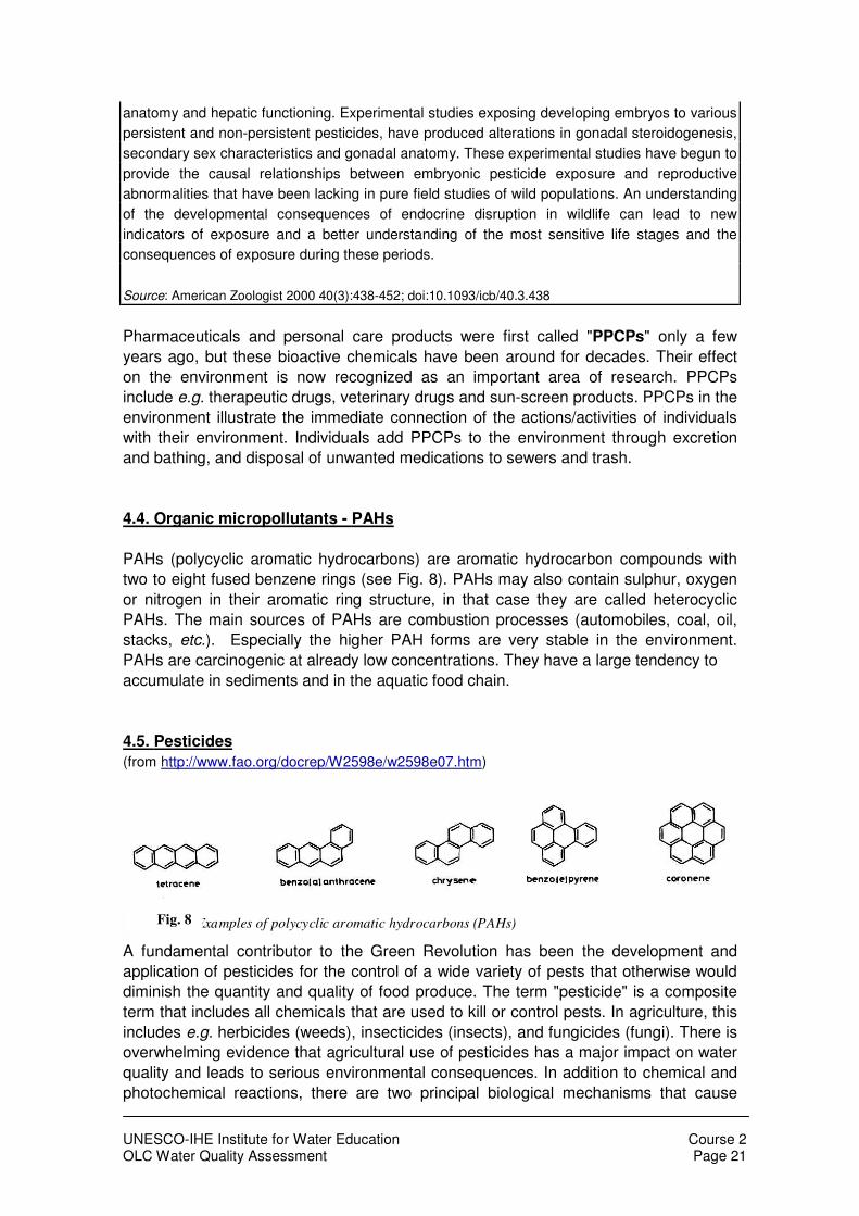
4.4. Organic micropollutants - PAHs
PAHs (polycyclic aromatic hydrocarbons) are aromatic hydrocarbon compounds with
two to eight fused benzene rings (see Fig. 8). PAHs may also contain sulphur, oxygen
or nitrogen in their aromatic ring structure, in that case they are called heterocyclic
PAHs. The main sources of PAHs are combustion processes (automobiles, coal, oil,
stacks, etc.). Especially the higher PAH forms are very stable in the environment.
PAHs are carcinogenic at already low concentrations. They have a large tendency to
accumulate in sediments and in the aquatic food chain.
4.5. Pesticides
(from http://www.fao.org/docrep/W2598e/w2598e07.htm)
A fundamental contributor to the Green Revolution has been the development and
application of pesticides for the control of a wide variety of pests that otherwise would
diminish the quantity and quality of food produce. The term "pesticide" is a composite
term that includes all chemicals that are used to kill or control pests. In agriculture, this
includes e.g. herbicides (weeds), insecticides (insects), and fungicides (fungi). There is
overwhelming evidence that agricultural use of pesticides has a major impact on water
quality and leads to serious environmental consequences. In addition to chemical and
photochemical reactions, there are two principal biological mechanisms that cause
Fig.5.4. Examples of polycyclic aromatic hydrocarbons (PAHs) Fig. 8
UNESCO-IHE Institute for Water Education Course 2 OLC Water Quality Assessment Page 22
degradation of pesticides. These are (1) microbiological processes in soils and water
and (2) metabolism of pesticides that are ingested by organisms as part of their food
supply. While both processes are beneficial in the sense that pesticide toxicity is
reduced, metabolic processes do cause adverse effects in, for example, fish. Energy
used to metabolize pesticides and other xenobiotics is not available for other body
functions and can seriously impair growth and reproduction of the organism.
PART 2 – BIOACCUMULATION
Bioaccumulation is the increase in
concentration of a substance in living
organisms as they take in contaminated air,
water, or food. As bigger animals eat smaller
animals, the level of contamination in the food
is added to the level of contamination already
in their body, and we end up with
biomagnification. Thus:
• Bioaccumulation: increase in
concentration of a pollutant from the
environment to the first organism in a
food chain (e.g. in algae)
• Biomagnification: increase in
concentration of a pollutant from one
link in a food chain to another
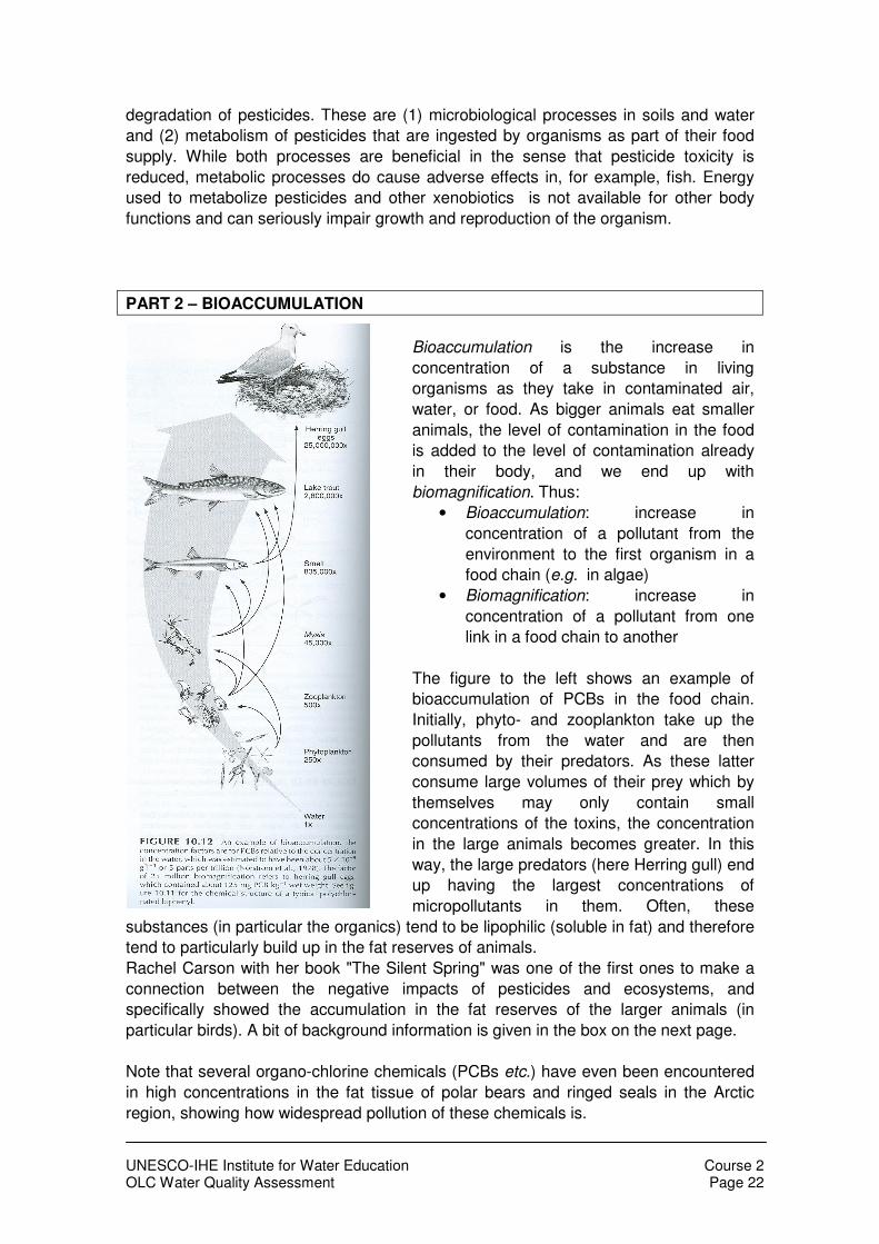
The figure to the left shows an example of
bioaccumulation of PCBs in the food chain.
Initially, phyto- and zooplankton take up the
pollutants from the water and are then
consumed by their predators. As these latter
consume large volumes of their prey which by
themselves may only contain small
concentrations of the toxins, the concentration
in the large animals becomes greater. In this
way, the large predators (here Herring gull) end
up having the largest concentrations of
micropollutants in them. Often, these
substances (in particular the organics) tend to be lipophilic (soluble in fat) and therefore
tend to particularly build up in the fat reserves of animals.
Rachel Carson with her book "The Silent Spring" was one of the first ones to make a
connection between the negative impacts of pesticides and ecosystems, and
specifically showed the accumulation in the fat reserves of the larger animals (in
particular birds). A bit of background information is given in the box on the next page.
Note that several organo-chlorine chemicals (PCBs etc.) have even been encountered
in high concentrations in the fat tissue of polar bears and ringed seals in the Arctic
region, showing how widespread pollution of these chemicals is.

UNESCO-IHE Institute for Water Education Course 2 OLC Water Quality Assessment Page 23
Rachel Carson’s Silent Spring and the Beginning of the Environmental Movement
(http://classwebs.spea.indiana.edu/bakerr/v600/rachel_carson_and_silent_spring.htm)
Introduction
When Rachel Carson's Silent Spring was published in 1962, it generated a storm of controversy
over the use of chemical pesticides. Miss Carson's intent in writing Silent Spring was to warn
the public of the dangers associated with pesticide use. Throughout her book are numerous
case studies documenting the harmful effects that chemical pesticides have on the environment.
Along with these facts, she explains how in many instances the pesticides have done more
harm than good in eradicating the pests they were designed to destroy. In addition to her
reports on pesticide use, Miss Carson points out that many of the long-term effects that these
chemicals may have on the environment, as well as on humans, are still unknown. Her book as
one critic wrote, "dealt pesticides a sharp blow" (Senior Scholastic 1962). The controversy
sparked by Silent Spring led to the enactment of environmental legislation and the
establishment of government agencies to better regulate the use of these chemicals.
Miss Carson first became aware of the effects of chemical pesticides on the natural environment
while working for the U.S. Bureau of Fisheries. Of particular concern to her was the
government’s use of chemical pesticides such as DDT. She was familiar with early studies of
DDT and knew of its dangers and lasting effects on the environment. According to Miss Carson,
"the more I learned about the use of pesticides, the more appalled I became. I realized that here
was the material for a book. What I discovered was that everything which meant most to me as
a naturalist was being threatened, and that nothing I could do would be more important." Thus,
Silent Spring was written to alert the public and stir people to action against the abuse of
chemical pesticides (Time 2000).
Impact of Silent Spring
When excerpts of Silent Spring first began appearing in The New Yorker magazine in June
1962, they caused uproar and brought a "howl of indignation" from the chemical industry.
Supporters of the pesticide industry argued that her book gave an incomplete picture because it
did not say anything about the benefits of using pesticides. An executive of the American
Cyanamid Company complained, "if man were to faithfully follow the teachings of Miss Carson,
we would return to the Dark Ages, and the insects and diseases and vermin would once again
inherit the earth." Chemical manufacturers began undertaking a more aggressive public
relations campaign to educate the public on the benefits of pesticide use. Monsanto, for
example, published and distributed 5,000 copies of a brochure "parodying" Silent Spring entitled
"The Desolate Year," which explained how chemical pesticides were largely responsible for the
virtual eradication of diseases such as malaria, yellow fever, sleeping sickness, and typhus in
the United States and throughout the world, and that without the assistance of pesticides in
agricultural production millions around the world would suffer from malnutrition or starve to
death (NRDC 1997).

UNESCO-IHE Institute for Water Education Course 2 OLC Water Quality Assessment Page 24
PART 3 – ECOTOXICOLOGY
The term ecotoxicology was coined by René Truhaut in 1969 who defined it as "the
branch of toxicology concerned with the study of toxic effects, caused by natural or
synthetic pollutants, to the constituents of ecosystems, animal (including human),
vegetable and microbial, in an integral context”. Ecotoxicology is the integration of
toxicology and ecology or, as the book of Chapman suggests: ecology in the presence
of toxicants”. It aims to quantify the effects of stressors upon natural populations,
communities, or ecosystems. Ecotoxicology incorporates aspects of ecology,
toxicology, physiology, molecular biology, analytical chemistry and many other
disciplines. The ultimate goal of this approach is to be able to predict the effects of
pollution so that the most efficient and effective action to prevent or remediate any
detrimental effect can be identified. In ecosystems that are already impacted by
pollution, ecotoxicological studies can inform as to the best course of action to restore
ecosystem services and functions efficiently and effectively.
An ecotoxicological assessment usually consists of two main parts, as shown in Fig. 8
(taken from Schwarzenbach et al., 2006, Science Vol 313):
• Exposure assessment: based on the environmental fate of chemicals; one can
calculate the bioavailability of substances (what is the concentration of a
chemical that is really available to an organism?)
• Toxicological assessment: what is the effect of the bioavailable concentration
on an organism?
Drinking water and food guidelines are then usually determined using a risk-based
assessment. Generally, Risk = Exposure (amount and/or duration) × Toxicity.
We cannot go into too many details because ecotoxicology is a whole science domain
on its own, but below follows some general information about both steps.
Steps taken during exposure assessment:
• One will calculate the distribution or so-called partitioning over different
compartments (solid matter, water, gas, biota). For example: how much Cd
ends up in the water, how much ends up in the sediment, how much is taken up
by the water plants, etc.? This will depend on phenomena such as precipitation,
settling of solids onto which metals might be adsorbed, if chemicals dissolve
easily in water (hydrophylic) or not (hydrophobic), etc.
• One will also look into the degradational process of chemicals. "Degradates"
may have greater, equal or lower toxicity than the parent compound. As an
example, DDT degrades to DDD and DDE. The persistence of chemicals is
usually measured as their half-life (time required for the ambient concentration
to decrease by 50%). Persistence is determined by biotic and abiotic
degradational processes. Biotic processes are biodegradation and metabolism;
abiotic processes are mainly hydrolysis (reaction with water), photolysis
(degradation in the light), and oxidation.

UNESCO-IHE Institute for Water Education Course 2 OLC Water Quality Assessment Page 25
Fig. 8. Steps taken in ecotoxicological assessment
• In toxicology, the median lethal dose, LD50 (abbreviation for “Lethal Dose, 50%”),
and LC50 (Lethal Concentration, 50%) of a toxic substance is the dose required
to kill half the members of a tested population. Typically, the LD50 of a substance
is given in milligrams per kilogram of body weight. Stating it this way allows the
relative toxicity of different substances to be compared, and normalizes for the
variation in the size of the animals exposed. Note that some pollutants can be
protagonistic, meaning in combination they enhance toxicity towards the
organism, or they can be antagonistic, where their toxic effects decrease in
combination, cause less threat to the organism.
Please refer to Chapter 5.7 in Chapman for further insight into methods for assessing
toxic pollution.

UNESCO-IHE Institute for Water Education Course 2 OLC Water Quality Assessment Page 26
PART 4 – MICROPOLLUTANTS IN AQUATIC SEDIMENTS
Aquatic sediments can have different sources:
• Allogenic (or allochthonous) material, deriving from outside the system. These
include mainly sand, silt and clay transported by rivers;
• Endogenic minerals, from processes in the water system (sedimentation of
carbonates, algae, etc.), and
• Authigenic (or authochtonous) minerals, which are formed within the sediment by
physico-chemical (oxidation, precipitation, etc.) and microbiological processes.
Any aquatic sediment in a river, lake, estuary or sea consists of a complex mixture of
discrete minerals and organic compounds to which a number of ions are more or less
tightly bound. For different aquatic ecosystems, the composition of sediments can be of
a highly variable nature, with organic carbon fractions ranging from 0.1% in deep
oceans up to >20% in dredged materials, and grain sizes between 1 and 10-7 mm.
A major fraction of the sediment minerals consists of quartz and feldspars; these are
almost exclusively to be found in the sand (> 63 µm) and silt (between 2 and 63 µm)
fraction. These non-clay minerals are chemically rather inert. In contrast, clays (< 2µm)
are very active in the adsorption of dissolved compounds. This is due to their large
specific surface area and their specific chemical layer structure. Clays are capable to
adsorb large quantities of both cations and anions, as well as organic compounds.
Sediments as “storage reservoirs” for micropollutants
Aquatic sediments commonly form the largest reservoir for micropollutants.
Micropollutants in aquatic ecosystems have a relatively large tendency to be adsorbed
onto suspended matter and sediments. This tendency can quantitatively be expressed
with the so-called Partition coefficient between water and sediment. The Partition
coefficient (L/kg) is defined as the µg micropollutant/kg particulate matter divided by the
µg/L present in the water phase. Some typical values for micropollutants are presented
in Table 2.
Table 2. Partition coefficients P (L/kg) of some chemicals
Heavy metals 104 - 105
Benzo(a)pyrene (PAH) 104 – 105
PCBs 105 – 106
Methoxychlor 104
Naphthalene 103
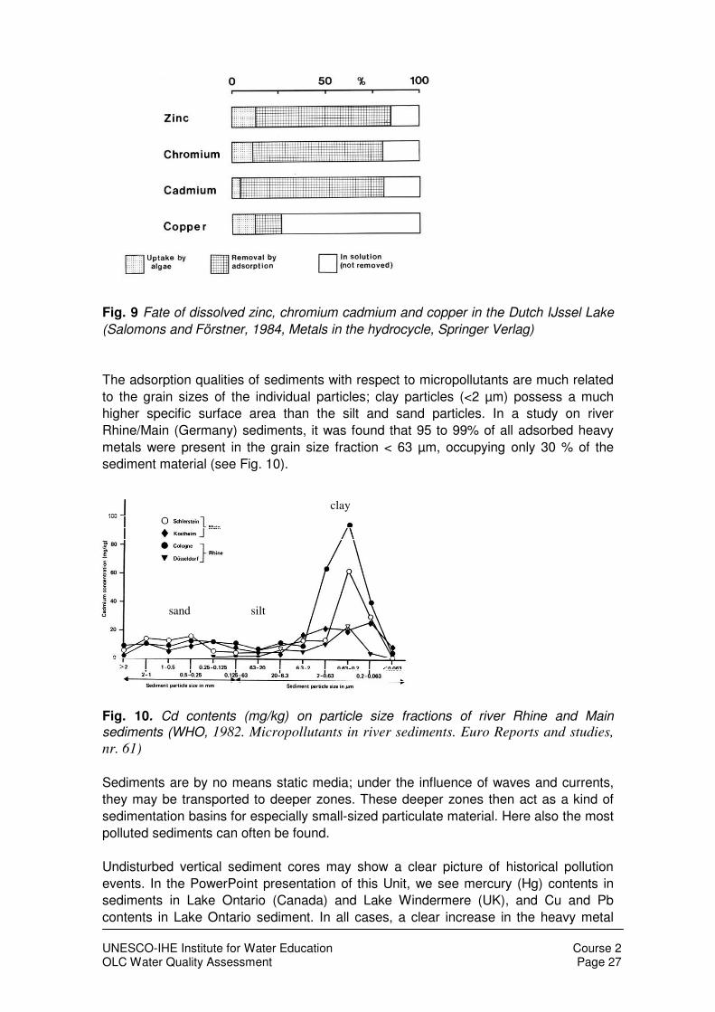
Thus, for chemicals such as heavy metals and PCBs, more than 50% can easily be
adsorbed onto particulate matter (see Fig. 9), and thus be "lost" due to sedimentation if
the river flow decreases. This mechanism is responsible for the deposition of pollutants
in lakes and stagnant rivers, which then serve as sedimentation basins. The above
mechanism is also a major reason for the potential harm of micropollutants, i.e. by
accumulation in the fatty tissue (liver, kidney, etc.) of organisms, and also of
biomagnification in the food chain. Here, higher organisms (fish, birds, men) feeding on
lower organisms (phyto- and zooplankton) may build up toxic, high levels.
UNESCO-IHE Institute for Water Education Course 2 OLC Water Quality Assessment Page 27
Fig. 9 Fate of dissolved zinc, chromium cadmium and copper in the Dutch IJssel Lake
(Salomons and Förstner, 1984, Metals in the hydrocycle, Springer Verlag)
The adsorption qualities of sediments with respect to micropollutants are much related
to the grain sizes of the individual particles; clay particles (<2 µm) possess a much
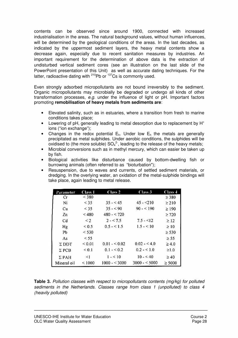
higher specific surface area than the silt and sand particles. In a study on river
Rhine/Main (Germany) sediments, it was found that 95 to 99% of all adsorbed heavy
metals were present in the grain size fraction < 63 µm, occupying only 30 % of the
sediment material (see Fig. 10).
Fig. 10. Cd contents (mg/kg) on particle size fractions of river Rhine and Main
sediments (WHO, 1982. Micropollutants in river sediments. Euro Reports and studies,
nr. 61)
Sediments are by no means static media; under the influence of waves and currents,
they may be transported to deeper zones. These deeper zones then act as a kind of
sedimentation basins for especially small-sized particulate material. Here also the most
polluted sediments can often be found.
Undisturbed vertical sediment cores may show a clear picture of historical pollution
events. In the PowerPoint presentation of this Unit, we see mercury (Hg) contents in
sediments in Lake Ontario (Canada) and Lake Windermere (UK), and Cu and Pb
contents in Lake Ontario sediment. In all cases, a clear increase in the heavy metal
sand silt
clay
UNESCO-IHE Institute for Water Education Course 2 OLC Water Quality Assessment Page 28
contents can be observed since around 1900, connected with increased
industrialisation in the areas. The natural background values, without human influences,
will be determined by the geological conditions of the areas. In the last decades, as
indicated by the uppermost sediment layers, the heavy metal contents show a
decrease again, especially due to recent sanitation measures by industries. An
important requirement for the determination of above data is the extraction of
undisturbed vertical sediment cores (see an illustration on the last slide of the
PowerPoint presentation of this Unit) as well as accurate dating techniques. For the
latter, radioactive dating with 210Pb or 137Cs is commonly used.
Even strongly adsorbed micropollutants are not bound irreversibly to the sediment. Organic micropollutants may microbially be degraded or undergo all kinds of other transformation processes, e.g. under the influence of light or pH. Important factors promoting remobilisation of heavy metals from sediments are:
• Elevated salinity, such as in estuaries, where a transition from fresh to marine conditions takes place;
• Lowering of pH, generally leading to metal desorption due to replacement by H+ ions (“ion exchange”);
• Changes in the redox potential Eh. Under low Eh the metals are generally precipitated as metal sulphides. Under aerobic conditions, the sulphides will be oxidised to (the more soluble) SO4
2-, leading to the release of the heavy metals;
• Microbial conversions such as in methyl mercury, which can easier be taken up by fish.
• Biological activities like disturbance caused by bottom-dwelling fish or burrowing animals (often referred to as “bioturbation");
• Resuspension, due to waves and currents, of settled sediment materials, or dredging. In the overlying water, an oxidation of the metal-sulphide bindings will take place, again leading to metal release.
Table 3. Pollution classes with respect to micropollutants contents (mg/kg) for polluted
sediments in the Netherlands. Classes range from class 1 (unpolluted) to class 4
(heavily polluted)

UNESCO-IHE Institute for Water Education Course 2 OLC Water Quality Assessment Page 29
Sediment quality guidelines
In the Netherlands, sediment quality has been divided into four classes; see Table 3.
More recently, Consensus based Sediment Quality Guidelines for Freshwater are used,
based on ecotoxicological guidelines; see Table hereunder.
Action List for Unit 4
− Look and listen to the Powerpoint presentation available under “Lecture”.
− Read chapter 3.8 Heavy metals, 3.9 Organic micropollutants and 5.7 Chemical
monitoring in Chapman (1996)
− Go to http://cfpub.epa.gov/ecotox/ from the EPA (US Environmental Protection
Agency) and perform a quick query on a chemical of your choice. You will see the
vast amount of information that has been reported.
− You can read more about pesticides under
http://www.fao.org/docrep/W2598e/w2598e07.htm
Further reading
Stanley Dodson, Introduction to Limnology, 2005, McGraw Hill

UNESCO-IHE Institute for Water Education Course 2 OLC Water Quality Assessment Page 30
Unit 5 – Aquatic ecosystems
Aquatic ecosystems are features in the landscape that participate in the processing
and transport of materials (sediments, pollutants, nutrients, organic matter) as these
materials move downstream from continents to oceans. This ability to process, retain,
or export nutrients, sediments, or pollutants is controlled in part by the physical
structure of the ecosystems (e.g. flowing vs. still water, stratification), by food web
structure and terrestrial inputs, and by nutrient dynamics.
In this unit, we will examine these things: 1. Processing of terrestrial inputs and food
web structure and 2. Nutrient processing, especially as it relates to eutrophication.
5.1. Introduction: Definition of aquatic systems and types
Watch the following movie on aquatic food webs:
http://www.youtube.com/watch?v=roRQQZlGIvM
An aquatic ecosystem is any watery environment, from small to large (i.e. from ponds
to oceans), running or still (rivers or lakes) that contain a group of interacting organisms
(plants, animals, microbes) that are dependent on one another and their water
environment for energy and food (carbon), nutrients (e.g., nitrogen and phosphorus)
and shelter.
Familiar examples are ponds, lakes and rivers, but aquatic ecosystems also include
areas such as floodplains and wetlands, which are flooded with water for all or only
parts of the year, highly polluted waters, and even thermal springs. Our health, human
livelihoods, recreation, and many of our activities are dependent on aquatic
ecosystems. Most of the water that we drink is taken from lakes or rivers, as well as
many food sources such as fish and shellfish. These activities are impaired when these
systems are unhealthy. Here, we will examine some ways in which ecosystems
function ecologically, in food web structure and dynamics, and in nutrient pathways
involved in eutrophication.
5.2. Food webs
Aquatic ecosystems usually contain a wide variety of life forms including autotrophs
and heterotrophs. Autotrophs are organisms that create their own energy from
inorganic sources (e.g. carbon dioxide (CO2) and water); this "photosynthesis" is one of
the dominant forms of autotrophy on Earth. Primary producers are organisms that
photosynthesize; they include algae, cyanobacteria, and higher plants such as sea
grass, bulrushes, cattails, reeds and other macrophytes.
Heterotrophs are organisms that depend on carbon that was previously fixed by
autotrophs. They respire this carbon, consuming oxygen to oxidize organic carbon
molecules back into carbon dioxide. Heterotrophs include a wide variety of organisms
including: small zooplankton that generally feed on phytoplankton, fish, birds, and man.
The food web (depicted in the PowerPoint presentation) is a simplified way of
understanding the process by which organisms in higher trophic levels gain energy by
consuming organisms at lower trophic levels. Because photosynthesis captures light
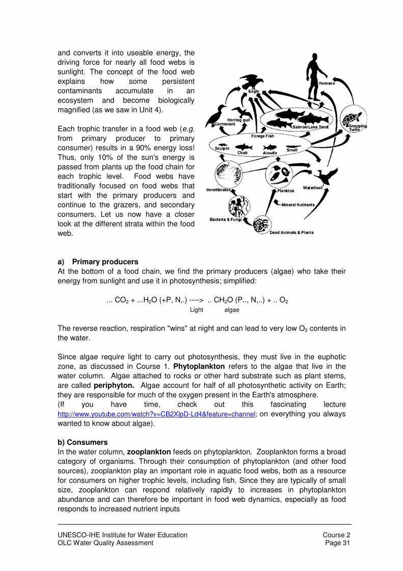
UNESCO-IHE Institute for Water Education Course 2 OLC Water Quality Assessment Page 31
and converts it into useable energy, the
driving force for nearly all food webs is
sunlight. The concept of the food web
explains how some persistent
contaminants accumulate in an
ecosystem and become biologically
magnified (as we saw in Unit 4).
Each trophic transfer in a food web (e.g.
from primary producer to primary
consumer) results in a 90% energy loss!
Thus, only 10% of the sun's energy is
passed from plants up the food chain for
each trophic level. Food webs have
traditionally focused on food webs that
start with the primary producers and
continue to the grazers, and secondary
consumers. Let us now have a closer
look at the different strata within the food
web.
a) Primary producers
At the bottom of a food chain, we find the primary producers (algae) who take their
energy from sunlight and use it in photosynthesis; simplified:
... CO2 + ...H2O (+P, N,.) ----> .. CH2O (P.., N,..) + .. O2
Light algae
The reverse reaction, respiration "wins" at night and can lead to very low O2 contents in
the water.
Since algae require light to carry out photosynthesis, they must live in the euphotic
zone, as discussed in Course 1. Phytoplankton refers to the algae that live in the
water column. Algae attached to rocks or other hard substrate such as plant stems,
are called periphyton. Algae account for half of all photosynthetic activity on Earth;
they are responsible for much of the oxygen present in the Earth's atmosphere.
(If you have time, check out this fascinating lecture
http://www.youtube.com/watch?v=CB2XlpD-Ld4&feature=channel; on everything you always
wanted to know about algae).
b) Consumers
In the water column, zooplankton feeds on phytoplankton. Zooplankton forms a broad
category of organisms. Through their consumption of phytoplankton (and other food
sources), zooplankton play an important role in aquatic food webs, both as a resource
for consumers on higher trophic levels, including fish. Since they are typically of small
size, zooplankton can respond relatively rapidly to increases in phytoplankton
abundance and can therefore be important in food web dynamics, especially as food
responds to increased nutrient inputs

UNESCO-IHE Institute for Water Education Course 2 OLC Water Quality Assessment Page 32
c) Predators
These can be fish, birds, or even higher
up in the food chain (such as the polar
bears). These can be planktivorous (either
phyto or zoo) or piscivorous (meaning
they eat smaller fish). The type of predator
that is present in the water will determine
largely the species composition and
abundance of the prey and others. In Lake
Victoria, for instance, many fish species
have been identified, with the Nile Perch
being the one most used commercially
(almost 80,000 tons of catch/year).
However, the Nile Perch is an exotic
species to the lake and is responsible for serious depletion in the populations of native
cichlads. (Source: Lake Victoria by J. Awange & O On’gan’ga, 2006 Springer).
d) Top-Down and Bottom-up control of food webs.
The phrase "top-down" and "bottom-up" control refers to the question of whether
primary production (or a prey species) is controlled by consumers (top-down control) or
by nutrients or light (bottom-up control). This question has been especially important in
understanding and mitigating eutrophication and overfishing.
In aquatic systems, nutrient availability is the most commonly considered factor, though
researchers also consider light as an important "bottom-up" factor, especially as
excess nutrients can cause algal blooms which shade benthic macrophytes. Nutrient
availability can determine the presence or absence of species. Further, the diversity
and abundance of phytoplankton determines the abundance and diversity of
zooplankton. "Top-down" control refers to situations where the abundance, diversity
or biomass of lower trophic levels are controlled by consumers at higher trophic levels.
In a "trophic cascade", predators induce effects that cascade down the food chain and
affect biomass of organisms at least two links away. For instance, fish predation of
zooplankton can increase phytoplankton biomass indirectly by eliminating zooplankton
grazing pressure on phytoplankton, thus exerting top-down control on phytoplankton
abundance.
5.3. Eutrophication - or why we worry about nutrients
We have already been talking a lot about pollution and problems with nutrients. Now let
us have a closer look at one of these problems: eutrophication. This term generally
refers to an overgrowth of algae and water plants, due to high inputs of the nutrients N
and P, which are essential for algae and plant growth. In order to understand
eutrophication, we need to look at the so called trophic states (see PowerPoint for
photographs). Lakes with low nutrient contents are usually oligotrophic; they are
characterized by high light visibility (see Course 3; for field measurements) and low
chlorofyll-a contents (the cells active in the primary production of algae and plants).
Lake Baikal (Russia) is an example of such a lake; high alpine lakes and many tropical
lakes such as the East African Rift lakes are other examples. Mesotrophic systems
have slightly higher nutrient contents, but are fairly rare, since they usually represent a

UNESCO-IHE Institute for Water Education Course 2 OLC Water Quality Assessment Page 33
transitional situation from oligotropic towards eutrophic systems. Eutrophic and
hypereutrophic systems are the ones we are mostly concerned about where large
amounts of nutrients cause tremendous algal blooms and excessive macrophyte
growth, causing anaerobic conditions in the water at night, leading to massive fish kills
(see Fig. 11).
Eutrophication was first evident in lakes and rivers as they became choked with
excessive growth of rooted plants and floating algal scums, prompting intense study in
the 1960's-70's and culminating in the scientific basis for banning phosphate
detergents (a major source of P, the most frequent culprit in eutrophication of lakes)
and upgrading sewage treatment to reduce wastewater N and P discharges to inland
waters. Symptoms of eutrophication in estuaries and other coastal marine ecosystems
(where N is the most frequent contributor to eutrophication) were clearly evident by the
1980's, as human activities
doubled the transport of N and
tripled the transport of P from
Earth's land surface to its
oceans. Eutrophication has
emerged as a key human
stressor on the world's coastal
ecosystems.
Fig. 11. Fish Kill in the Salton Sea as a result of eutrophication
Some phytoplankton species produce toxic chemicals that can impair respiratory,
nervous, digestive and reproductive system function, and even cause death of fish,
shellfish, seabirds, mammals, and humans. The economic impacts of harmful algal
blooms can be severe as tourism is lost and shellfish harvesting and fishing are closed
across increasingly widespread regions. Proposed solutions to the eutrophication
problem are multidimensional and include actions to restore wetlands and riparian
buffer zones between farms and surface waters, reduce livestock densities, improve
efficiencies of fertilizer applications, treat urban runoff from streets and storm drains,
reduce N emissions from vehicles and power plants, ban P-containing detergents, and
further increase the efficiency of N and P removal from wastewaters.
5.4. The importance of N:P Ratio
The nutrient requirement necessary for phytoplankton growth is called the Redfield
ratio (taken from research by Redfield in 1958). This ratio relates nutrient uptake by
phytoplankton to primary production. The C:N:P ratio for phytoplankton is generally
considered to be 106:16:1. This means that for 106 moles of carbon fixed by
photosynthesis, the algal cell also requires 16 moles of N and 1 mole of P, or in grams,
about 10 g N per 1 g P; the algae cells will take this up from the water environment, or
in the case of nitrogen may also fix it from the atmosphere.
The key implication of this ratio is that the rates at which nutrients are added to a
system affect the limiting nutrient. The limiting nutrient is the one that is in shortest
UNESCO-IHE Institute for Water Education Course 2 OLC Water Quality Assessment Page 34
supply, so that when added, it stimulates growth in phytoplankton. If the Redfield ratio
of the nutrient inputs is higher than 10:1 (N:P > 10:1), the ecosystem is considered to
be limited by phosphorus. This is the case in most fresh water lakes and rivers. In
contrast, if the ratio of the nutrient loads to an ecosystem is below the Redfield ratio
(N:P < 10:1), the system is nitrogen limited, e.g. in many coastal waters and estuaries.
Eutrophication abatement thus often concentrates on P limitation, also because for N,
there can be alternative sources: biological N fixation.
Whole-lake experiments have been carried out for experimental lakes in Canada; this
is illustrated in the PowerPoint presentation. A curtain divided the two sides of the lake
and fertilizer was added in different proportions to each side of the lake.
Read more about Canada’s whole lake experiments:
http://www.sciencemag.org/cgi/reprint/322/5906/1316.pdf?ck=nck
Action List for Unit 6
• Read chapter 6.5 and 7 in Chapman et al.
• Browse through your local newspaper and search for articles related to
eutrophication. See if you can find out the economic impact of eutrophication (i.e. the
cost to remove excessive sea weeds from harbour regions) and report it on the
discussion board.
YouTube illustrations
Watch the following movie on aquatic food webs:
http://www.youtube.com/watch?v=roRQQZlGIvM
Further reading
Planning and Management of Lakes and Reservoirs: An Integrated Approach to
Eutrophication:
http://www.unep.or.jp/ietc/publications/techpublications/techpub-11/index.asp#1
Please refer to the comprehensive report on the current state of lake eutrophication by
the UNEP:
http://www.unep.or.jp/ietc/publications/short_series/lakereservoirs-3/2.asp

UNESCO-IHE Institute for Water Education Course 2 OLC Water Quality Assessment Page 35
Unit 6 – Water quality modelling
As we have seen in Unit 1 of this course, characterising the water quality of for
instance a lake is a challenging task, because there are:
• Temporal variations
• Spatial variations
• Many different water quality variables and standards
• Relations between water quality variables such as BOD/DO, N/phytoplankton, ...
One tool which can help us to get a more comprehensive view of the water quality of
lakes and rivers is mathematical modelling. Once a reliable model has been developed,
it is capable of predicting modelled water quality variables for different times and
locations.
A general approach can be seen in Fig. 12. Developing a water quality model usually
consists of two separate exercises:
• Hydrodynamic modelling: this means modelling the transport of water and
substances (by flow, advection, diffusion, ...)
• Water quality modelling: modelling conversion processes of substances (e.g.
nitrification, oxygen consumption when BOD is being degraded, ...)
One will usually start by developing a conceptual model. This includes setting the
(physical) boundary conditions (e.g. are you only interested in the lake water or do you
also want to include sediment processes), the level of detail that you are interested in
(1D, 2D or 3D; monthly average values or hourly predictions) and a selection of
relevant water quality variables (only interested in BOD-DO or also nutrients,
phytoplankton, ...). Once this has been done, the hydrodynamic and water quality
models can be developed. These cannot be used at once, but first need to be
calibrated. This means that model predictions will be fitted to real measured values by
fine-tuning model equations and/or parameter values. Once that has been done, a
validation/verification is usually required, meaning that the model results are checked
against another, independent set of measured data (i.e. different from the one used for
calibration). Then the model is ready and can be used for scenario analyses, i.e. what
happens if we reduce the nutrient load, what will happen with phytoplankton
concentrations when the temperature rises because of global warming, etc.
This Unit is an optional unit, meaning that you are free to continue looking into this
matter or not. There are also no lecture notes; only a Power Point presentation (without
audio) by dr. Kelderman and a set of seven selected peer-reviewed journal papers: six
on river water quality modelling and one on lake modelling. They are available under
Unit 6 - Supplementary Materials. There is a logical sequence in the papers, so if you
are interested, please follow the numbering.

UNESCO-IHE Institute for Water Education Course 2 OLC Water Quality Assessment Page 36
Fig. 12. General approach to water quality modelling