Coupling functions: Universal insights into dynamical ...

Coupling functions: Universal insights into dynamicalinteraction mechanisms

Tomislav StankovskiFaculty of Medicine, Ss Cyril and Methodius University, 50 Divizija 6, Skopje 1000, Macedoniaand Department of Physics, Lancaster University, Lancaster, LA1 4YB, United Kingdom

Tiago PereiraDepartment of Mathematics, Imperial College London, London SW7 2AZ, United Kingdomand Institute of Mathematical and Computer Sciences, University of Sao Paulo,Sao Carlos 13566-590, Brazil

Peter V. E. McClintock and Aneta StefanovskaDepartment of Physics, Lancaster University, Lancaster, LA1 4YB, United Kingdom

(published 6 November 2017)

The dynamical systems found in nature are rarely isolated. Instead they interact and influenceeach other. The coupling functions that connect them contain detailed information about thefunctional mechanisms underlying the interactions and prescribe the physical rule specifyinghow an interaction occurs. A coherent and comprehensive review is presented encompassing therapid progress made recently in the analysis, understanding, and applications of couplingfunctions. The basic concepts and characteristics of coupling functions are presented throughdemonstrative examples of different domains, revealing the mechanisms and emphasizing theirmultivariate nature. The theory of coupling functions is discussed through gradually increasingcomplexity from strong and weak interactions to globally coupled systems and networks. A varietyof methods that have been developed for the detection and reconstruction of coupling functionsfrom measured data is described. These methods are based on different statistical techniquesfor dynamical inference. Stemming from physics, such methods are being applied in diverseareas of science and technology, including chemistry, biology, physiology, neuroscience, socialsciences, mechanics, and secure communications. This breadth of application illustrates theuniversality of coupling functions for studying the interaction mechanisms of coupled dynamicalsystems.

DOI: 10.1103/RevModPhys.89.045001

CONTENTS

I. Introduction 2A. Coupling functions, their nature, and uses 2B. Significance for interacting systems more generally 3

1. Physical effects of interactions: Synchronization,amplitude, and oscillation death 3

2. Coupling strength and directionality 43. Coupling functions in general interactions 5

II. Basic Concept of Coupling Functions 5A. Principle meaning 5

1. Generic form of coupled systems 52. Coupling function definition 53. Example of coupling function and

synchronization 6B. History 6C. Different domains and usage 8

1. Phase coupling functions 82. Amplitude coupling functions 93. Multivariate coupling functions 104. Generality of coupling functions 11

D. Coupling functions revealing mechanisms 11E. Synchronization prediction with coupling functions 12

F. Unifying nomenclature 13III. Theory 13

A. Strong interaction 141. Two coupled oscillators 142. Comparison between approaches 17

B. Weak regime 171. Stable periodic orbit and its phase 182. Coupling function and phase reduction 193. Synchronization with external forcing 194. Phase response curve 205. Examples of the phase sensitivity function 21

C. Globally coupled oscillators 211. Coupling functions leading to multistability 222. Designing coupling functions for cluster

states and chimeras 223. Coupling functions with delay 234. Low-dimensional dynamics 235. Noise and nonautonomous effects 24

D. Networks of oscillators 241. Reduction to phase oscillators 242. Networks of chaotic oscillators 25

IV. Methods 26A. Inferring coupling functions 26

REVIEWS OF MODERN PHYSICS, VOLUME 89, OCTOBER–DECEMBER 2017

0034-6861=2017=89(4)=045001(50) 045001-1 © 2017 American Physical Society

https://doi.org/10.1103/RevModPhys.89.045001




B. Methods for coupling function reconstruction 271. Modeling by least-squares fitting 272. Dynamical Bayesian inference 283. Maximum likelihood estimation: Multiple

shooting 294. Random phase resetting method 315. Stochastic modeling of effective coupling

functions 316. Comparison and overview of the methods 32

C. Toward coupling function analysis 33D. Connections to other methodological concepts 34

1. Phase reconstruction procedures 342. Relation to phase response curve

in experiments 343. General effective connectivity modeling 35

V. Applications and Experiments 35A. Chemistry 35B. Cardiorespiratory interactions 37C. Neural coupling functions 39D. Social sciences 40E. Mechanical coupling functions 41F. Secure communications 42

VI. Outlook and Conclusion 43A. Future directions and open questions 43

1. Theory 432. Methods 433. Analysis 444. Integration theory applications 445. Applications 44

B. Conclusion 44Acknowledgments 45References 45

I. INTRODUCTION

A. Coupling functions, their nature, and uses

Interacting dynamical systems abound in science and tech-nology, with examples ranging from physics and chemistry,through biology and population dynamics, to communicationsand climate (Winfree, 1980; Haken, 1983; Kuramoto, 1984;Pikovsky, Rosenblum, and Kurths, 2001; Strogatz, 2003).The interactions are defined by two main aspects: structure

and function. The structural links determine the connections andcommunications between the systems or the topology of anetwork. The functions are quite special from the dynamicalsystems viewpoint as they define the laws by which the actionand coevolution of the systems are governed. The functionalmechanisms can lead to a variety of qualitative changes in thesystems. Depending on the coupling functions, the resultantdynamics can be quite intricate, manifesting a whole range ofqualitatively different states, physical effects, phenomena, andcharacteristics, including synchronization (Lehnertz and Elger,1998; Pikovsky, Rosenblum, and Kurths, 2001; Acebrón et al.,2005; Kapitaniak et al., 2012), oscillation and amplitude death(Saxena, Prasad, and Ramaswamy, 2012; Koseska, Volkov, andKurths, 2013a), birth of oscillations (Smale, 1976; Pogromsky,Glad, and Nijmeijer, 1999), breathers (MacKay and Aubry,1994), coexisting phases (Keller, Künzle, and Nowicki, 1992),fractal dimensions (Aguirre, Viana, and Sanjuán, 2009), net-work dynamics (Boccaletti et al., 2006;Arenas et al., 2008), andcoupling strength and directionality (Stefanovska and Bračič,

1999; Rosenblum and Pikovsky, 2001; Hlaváčkováá-Schindleret al., 2007;Marwan et al., 2007). Knowledge of such couplingfunction mechanisms can be used to detect, engineer, or predictcertain physical effects, to solve someman-made problems and,in living systems, to reveal their state of health and to investigatechanges due to disease.Coupling functions possess unique characteristics carrying

implications that go beyond the collective dynamics (e.g.,synchronization or oscillation death). In particular, the form ofthe coupling function can be used, not only to understand, butalso to control and predict the interactions. Individual units canbe relatively simple, but the nature of the coupling function canmake their collective dynamics particular, enabling specialbehavior. Additionally, there exist applications which dependjust and only on the coupling functions, including examples ofapplications in social sciences and secure communication.Given these properties, it is hardly surprising that cou-

pling functions have recently attracted considerable atten-tion within the scientific community. They have mediatedapplications, not only in different subfields of physics, butalso beyond physics, predicated by the development ofpowerful methods enabling the reconstruction of couplingfunctions from measured data. The reconstruction withinthese methods is based on a variety of inference techniques,e.g., least-squares and kernel smoothing fits (Rosenblumand Pikovsky, 2001; Kralemann et al., 2013), dynamicalBayesian inference (Stankovski et al., 2012), maximumlikelihood (multiple-shooting) methods (Tokuda et al.,2007), stochastic modeling (Schwabedal and Pikovsky,2010), and the phase resetting (Galán, Ermentrout, andUrban, 2005; Timme, 2007; Levnajić and Pikovsky, 2011).Both the connectivity between systems and the associated

methods employed for revealing it are often differentiated intostructural, functional, and effective connectivity (Friston,2011; Park and Friston, 2013). Structural connectivity isdefined by the existence of a physical link, such as anatomicalsynaptic links in the brain or a conducting wire betweenelectronic systems. Functional connectivity refers to thestatistical dependences between systems, such as, for exam-ple, correlation or coherence measures. Effective connectivityis defined as the influence one system exerts over another,under a particular model of causal dynamics. Importantly inthis context, the methods used for the reconstruction ofcoupling functions belong to the group of effective connec-tivity techniques, i.e., they exploit a model of differentialequations and allow for dynamical mechanisms—such as thecoupling functions themselves—to be inferred from data.Coupling function methods have been applied widely

(Fig. 1) and to good effect: in chemistry, for understanding,effecting, or predicting interactions between oscillatoryelectrochemical reactions (Miyazaki and Kinoshita, 2006;Kiss et al., 2007; Tokuda et al., 2007; Blaha et al., 2011;Kori et al., 2014); in cardiorespiratory physiology (Stankovskiet al., 2012; Iatsenko et al., 2013; Kralemann et al., 2013;Ticcinelli et al., 2017) for reconstruction of the humancardiorespiratory coupling function and phase resetting curve,for assessing cardiorespiratory time variability, and for study-ing the evolution of the cardiorespiratory coupling functionswith age; in neuroscience for revealing the cross-frequencycoupling functions between neural oscillations (Stankovski

Stankovski et al.: Coupling functions: Universal insights into …

Rev. Mod. Phys., Vol. 89, No. 4, October–December 2017 045001-2

et al., 2015); and polyrithmic behavior in neuronal circuits(Wojcik et al., 2014; Schwabedal, Knapper, and Shilnikov,2016); in social sciences for determining the function under-lying the interactions between democracy and economicgrowth (Ranganathan et al., 2014); for mechanical interactionsbetween coupled metronomes (Kralemann et al., 2008); and insecure communications where a new protocol was developedexplicitly based on amplitude coupling functions (Stankovski,McClintock, and Stefanovska, 2014).In parallel with their use to support experimental work,

coupling functions are also at the center of intense theoreticalresearch (Crawford, 1995; Daido, 1996a; Strogatz, 2000;Acebrón et al., 2005). Particular choices of coupling functionscan allow for a multiplicity of singular synchronized states(Komarov and Pikovsky, 2013). Coupling functions areresponsible for the overall coherence in complex networksof nonidentical oscillators (Luccioli and Politi, 2010; Pereira

et al., 2013; Ullner and Politi, 2016) and for the formation ofwaves and antiwaves in coupled neurons (Urban andErmentrout, 2012). Coupling functions play important rolesin the phenomena resulting from interactions such as syn-chronization (Kuramoto, 1984; Daido, 1996a; Maia, Pereira,and Macau, 2015), amplitude and oscillation death (Aronson,Ermentrout, and Kopell, 1990; Koseska, Volkov, and Kurths,2013a; Zakharova, Kapeller, and Schöll, 2014; Schneideret al., 2015), the low-dimensional dynamics of ensembles(Watanabe and Strogatz, 1993; Ott and Antonsen, 2008), andclustering in networks (Ashwin and Timme, 2005; Kori et al.,2014). The findings of these theoretical works are furtherfostering the development of methods for coupling functionreconstruction, paving the way to additional applications.

B. Significance for interacting systems more generally

An interaction can result from a structural link throughwhichcausal information is exchanged between the system and one ormore other systems (Winfree, 1980; Haken, 1983; Kuramoto,1984; Pikovsky, Rosenblum, and Kurths, 2001; Strogatz,2003). Often it is not so much the nature of the individualparts and systems, but how they interact that determines theircollective behavior. One example is circadian rhythms, whichoccur across different scales and organisms (DeWoskin et al.,2014). The systems themselves can be diverse in nature—for example, they can be either static or dynamical,including oscillatory, nonautonomous, chaotic, or stochasticcharacteristics (Katok and Hasselblatt, 1997; Strogatz, 2001;Gardiner, 2004; Kloeden and Rasmussen, 2011; Landa, 2013;Suprunenko, Clemson, and Stefanovska, 2013). From theextensive set of possibilities, we focus in this review ondynamical systems, concentrating especially on nonlinearoscillators because of their particular interest and importance.

1. Physical effects of interactions: Synchronization, amplitude,and oscillation death

An intriguing feature is that their mutual interactions canchange the qualitative state of the systems. Thus they can causetransitions into or out of physical states such as synchroniza-tion, amplitude, or oscillation death, or quasisynchronizedstates in networks of oscillators.The existence of a physical effect is, in essence, defined by

the presence of a stable state for the coupled systems. Theirstability is often probed through a dimensionally reduceddynamics, for example, the dynamics of their phase differenceor of the driven system only. By determining the stability ofthe reduced dynamics, one can derive useful conclusionsabout the collective behavior. In such cases, the couplingfunctions describe how the stable state is reached and thedetailed conditions for the coupled systems to gain or losestability. In data analysis, the existence of the physical effectsis often assessed through measures that quantify, eitherdirectly or indirectly, the resultant statistical properties ofthe state that remains stable under interaction.The physical effects often converge to a manifold, such as a

limit cycle. Even after that, however, coupled dynamicalsystems can still exhibit their own individual dynamics,making them especially interesting objects for study.

FIG. 1. Examples of coupling functions used in chemistry,cardiorespiratory physiology, and secure communications todemonstrate their diversity of applications. (a) Coupling func-tions used for controlling and engineering the interactions of two(left) and four (right) nonidentical electrochemical oscillations.From Kiss et al., 2007. (b) Human cardiorespiratory couplingfunction Qe reconstructed from the phase dynamics of the heartφe and respiration φr phases. From Kralemann et al., 2013.(c) Schematic description of the coupling function encryptionprotocol. From Stankovski, McClintock, and Stefanovska, 2014.Multiple information signals are encrypted by modulating theparameters of linearly independent coupling functions between(chaotic) dynamical systems at the transmitter. These applicationsare discussed in detail in Sec. V.



Arguably, synchronization is the most studied of all suchphysical effects. It is defined as an adjustment of the rhythmsof the oscillators, caused by their weak interaction (Pikovsky,Rosenblum, and Kurths, 2001). Synchronization is the under-lying qualitative state that results from many cooperativeinteractions in nature. Examples include cardiorespiratorysynchronization (Kenner, Passenhofer, and Schwaberger,1976; Schäfer et al., 1998; Stefanovska et al., 2000), brainseizures (Lehnertz and Elger, 1998), neuromuscular activity(Tass et al., 1998), chemistry (Miyazaki and Kinoshita, 2006;Kiss et al., 2007), the flashing of fireflies (Buck and Buck,1968; Mirollo and Strogatz, 1990), and ecological synchro-nization (Blasius, Huppert, and Stone, 1999). Depending onthe domain, the observable properties, and the underlyingphenomena, several different definitions and types ofsynchronization have been studied. These include phasesynchronization, generalized synchronization, frequency syn-chronization, complete (identical) synchronization, lag syn-chronization, and anomalous synchronization (Ermentrout,1981; Kuramoto, 1984; Pecora and Carroll, 1990; Rulkovet al., 1995; Kocarev and Parlitz, 1996; Rosenblum, Pikovsky,and Kurths, 1996; Arnhold et al., 1999; Brown and Kocarev,2000; Pikovsky, Rosenblum, and Kurths, 2001; Blasius,Montbrio, and Kurths, 2003; Eroglu, Lamb, and Pereira,2017).Another important group of physical phenomena attribut-

able to interactions are those associated with oscillation andamplitude deaths (Bar-Eli, 1985; Mirollo and Strogatz, 1990;Prasad, 2005; Suárez-Vargas et al., 2009; Koseska, Volkov,and Kurths, 2013a; Zakharova et al., 2013; Schneider et al.,2015). Oscillation death is defined as a complete cessation ofoscillation caused by the interactions, when an inhomo-geneous steady state is reached. Similarly, in amplitude death,due to the interactions a homogeneous steady state is reachedand the oscillations disappear. The mechanisms leading tothese two oscillation quenching phenomena are mediated bydifferent coupling functions and conditions of interaction,including strong coupling (Mirollo and Strogatz, 1990; Zhai,Kiss, and Hudson, 2004), conjugate coupling (Karnatak,Ramaswamy, and Prasad, 2007), nonlinear coupling(Prasad et al., 2010), repulsive links (Hens et al., 2013),and environmental coupling (Resmi, Ambika, and Amritkar,2011). These phenomena are mediated, not only by the phasedynamics of the interacting oscillators, but also by theiramplitude dynamics, where the shear amplitude terms andthe nonisochronicity play significant roles. Coupling func-tions define the mechanism through which the interactioncauses the disappearance of the oscillations.There is a large body of earlier work in which physical

effects, qualitative states, or quantitative characteristics of theinteractions were studied, where coupling functions consti-tuted an integral part of the underlying interaction model,regardless of whether or not the term was used explicitly.Physical effects are very important and they are closelyconnected with the coupling functions. In such investigations,however, the coupling functions themselves were often notassessed or considered as entities in their own right. In simplewords, such investigations posed the question of whetherphysical effects occur; while for the coupling function inves-tigations the question is rather how they occur. Our emphasis

is therefore on coupling functions as entities, on the explora-tion and assessment of different coupling functions, and on theconsequences of the interactions.

2. Coupling strength and directionality

The coupling strength gives a quantitative measure of theinformation flow between the coupled systems. In an infor-mation-theoretic context, this is defined as the transfer ofinformation between variables in a given process. In atheoretical treatment the coupling strength is clearly thescaling parameter of the coupling functions. There is greatinterest in being able to evaluate the coupling strength forwhich many effective methods have been designed (Mormannet al., 2000; Rosenblum and Pikovsky, 2001; Paluš andStefanovska, 2003; Marwan et al., 2007; Bahraminasab et al.,2008; Staniek and Lehnertz, 2008; Chicharro and Andrzejak,2009; Smirnov and Bezruchko, 2009; Jamšek, Paluš, andStefanovska, 2010; Faes, Nollo, and Porta, 2011; Sun, Taylor,and Bollt, 2015). The dominant direction of influence, i.e., thedirection of the stronger coupling, corresponds to the direc-tionality of the interactions. Earlier, it was impossible to detectthe absolute value of the coupling strength, and a number ofmethods exist for detection only of the directionality throughmeasurements of the relative magnitudes of the interactions—for example, when detecting mutual information (Paluš andStefanovska, 2003; Staniek and Lehnertz, 2008; Smirnov andBezruchko, 2009), but not the physical coupling strength. Theassessment of the strength of the coupling and its predominantdirection can be used to establish if certain interactions exist atall. In this way, one can determine whether some apparentinteractions are in fact genuine, and whether the systems understudy are truly connected or not.When the coupling function results from a number of

functional components, its net strength is usually evaluated asthe Euclidian norm of the individual components’ couplingstrengths. Grouping the separate components, for example, theFourier components of periodic phase dynamics, one canevaluate the coupling strengths of the functional groups ofinterest. The latter could include the coupling strength eitherfrom one system or the other or from both of them. Thus onecan detect the strengths of the self-, direct, and commoncoupling components, or of the phase response curve (PRC)(Kralemann, Pikovsky, and Rosenblum, 2011; Iatsenko et al.,2013; Faes, Porta, and Nollo, 2015). In a similar way, theseideas can be generalized for multivariate coupling in networksof interacting systems.It is worth noting that, when inferring couplings even from

completely uncoupled or very weakly coupled systems, themethods will usually detect nonzero coupling strengths. Thisresults mainly from the statistical properties of the signals.Therefore, one needs to be able to ascertain whether thedetected coupling strengths are genuine, or spurious, justresulting from the inference method. To overcome thisdifficulty, one can apply surrogate testing (Paluš andHoyer, 1998; Schreiber and Schmitz, 2000; Andrzejak et al.,2003; Kreuz et al., 2004) which generates independent,uncoupled signals that have the same statistical propertiesas the original signals. The apparent coupling strengthevaluated for the surrogate signals should then reflect a “zero



level” of apparent coupling for the uncoupled signals. Bycomparison, one can then assess whether the detected cou-plings are likely to be genuine. This surrogate testing processis also important for coupling function detection; one firstneeds to establish whether a coupling relation is genuine andthen, if so, to try to infer the form of the coupling function.

3. Coupling functions in general interactions

This review is focused mainly on coupling functionsbetween interacting dynamical systems and especiallybetween oscillatory systems, because most studies to datehave been developed in that context. However, interactionshave also been studied in a broader sense for nonoscillatory,nondynamical systems spread over many different fields,including, for example, quantum plasma interactions(Marklund and Shukla, 2006; Shukla and Eliasson, 2011),solid state physics (Farid, 1997; Higuchi and Yasuhara, 2003;Zhang, 2013), interactions in semiconductor superlattices(Bonilla and Grahn, 2005), Josephson-junction interactions(Golubov, Kupriyanov, and IlIchev, 2004), laser diagnostics(Stepowski, 1992), interactions in nuclear physics (Guelfiet al., 2007; Mitchell, Richter, and Weidenmüller, 2010),geophysics (Murayama, 1982), space science (Feldstein,1992; Lifton et al., 2005), cosmology (Faraoni, Jensen, andTheuerkauf, 2006; Baldi, 2011), biochemistry (Khramov andBielawski, 2007), plant science (Doidy et al., 2012), oxy-genation and pulmonary circulation (Ward, 2008), cerebralneuroscience (Liao et al., 2013), immunology (Robertson andGhazal, 2016), biomolecular systems (Christen and VanGunsteren, 2008; Stamenović and Ingber, 2009; Dong, Liu,and Yang, 2014), gap junctions (Wei, Xu, and Lo, 2004), andprotein interactions (Jones and Thornton, 1996; Teasdale andJackson, 1996; Gaballo, Zanotti, and Papa, 2002; Okamoto,Bosch, and Hayashi, 2009). In many such cases, the inter-actions are different in nature. They are often structural andnot effective connections in the dynamics or the correspond-ing coupling functions may not have been studied in thiscontext before. Even though we do not discuss such systemsdirectly in this review, many of the concepts and ideas that weintroduce in connection with dynamical systems can also beuseful for the investigation of interactions more generally.

II. BASIC CONCEPT OF COUPLING FUNCTIONS

A. Principle meaning

1. Generic form of coupled systems

The main problem of interest is to understand the dynamicsof coupled systems from their building blocks. We start fromthe isolated dynamics

_x ¼ fðx; μÞ;

where f∶ Rm ×Rn → Rn is a differentiable vector field withμ being the set of parameters. For simplicity, whenever there isno risk of confusion, we will omit the parameters. Over the last50 years, developments in the theory of dynamical systemshave illuminated the dynamics of isolated systems. Forinstance, we understand their bifurcations, including those

that generate periodic orbits as well as those giving rise tochaotic motion. Hence we understand the dynamics of isolatedsystems in some detail.In contrast our main interest here is to understand the

dynamics of the coupled equations:

_x ¼ f1ðxÞ þ g1ðx; yÞ; ð1Þ

_y ¼ f2ðyÞ þ g2ðx; yÞ; ð2Þ

where f1;2 are vector fields describing the isolated dynamics(perhaps with different dimensions) and g1;2 are the couplingfunctions. The latter are our main objects of interest. Weassumed that they are at least twice differentiable.Note that we could also study this problem from an abstract

point of view by representing the equations as

_x ¼ q1ðx; yÞ; ð3Þ

_y ¼ q2ðx; yÞ; ð4Þ

where the functions q1;2 incorporate both the isolated dynam-ics and the coupling functions. This notation for inclusion ofcoupling functions, with no additive splitting between theinteractions and the isolated dynamics, can sometimes bequite useful (Aronson, Ermentrout, and Kopell, 1990; Pereiraet al., 2014). Examples include coupled cell networks(Ashwin and Timme, 2005) or the provision of full Fourierexpansions (Rosenblum and Pikovsky, 2001; Kiss, Zhai, andHudson, 2005) when inferring coupling functions from data.

2. Coupling function definition

Coupling functions describe the physical rule specifyinghow the interactions occur. Being directly connected with thefunctional dependences, coupling functions focus not so muchon whether there are interactions, but more on how theyappear and develop. For instance, the magnitude of the phasecoupling function directly affects the oscillatory frequencyand describes how the oscillations are being accelerated ordecelerated by the influence of the other oscillator. Similarly,if one considers the amplitude dynamics of interactingdynamical systems, the magnitude of the coupling functionwill prescribe how the amplitude is increased or decreased bythe interaction.A coupling function can be described in terms of its

strength and form. While the strength is a relatively well-studied quantity, this is not true of the form. It is the functionalform that has provided a new dimension and perspective,directly probing the mechanisms of interaction. In otherwords, the mechanism is defined by the functional formwhich, in turn, specifies the rule and process through whichthe input values are translated into output values, i.e., in termsof one system (system A) it prescribes how the input influencefrom another system (system B) gets translated into conse-quences in the output of system A. In this way the couplingfunction can describe the qualitative transitions betweendistinct states of the systems, e.g., routes into and out ofsynchronization. Decomposition of a coupling function pro-vides a description of the functional contributions from each



separate subsystem within the coupling relationship. Hence,the use of coupling functions amounts to much more than justa way of investigating correlations and statistical effects: itreveals the mechanisms underlying the functionality of theinteractions.

3. Example of coupling function and synchronization

To illustrate the fundamental role of coupling functions insynchronization, we considered a simple example of twocoupled phase oscillators (Kuramoto, 1984):

_ϕ1 ¼ ω1 þ ε1 sinðϕ2 − ϕ1Þ;_ϕ2 ¼ ω2 þ ε2 sinðϕ1 − ϕ2Þ; ð5Þ

where ϕ1, ϕ2 are the phase variables of the oscillators, ω1, ω2

are their natural frequencies, ε1, ε2 are the coupling strengthparameters, and the coupling functions of interest are bothtaken to be sinusoidal. (For further details including, inparticular, the choice of the coupling functions, see alsoSec. III.) Further, we consider coupling that depends only onthe phase difference ψ ¼ ϕ2 − ϕ1. In this case, from _ψ ¼_ϕ2 − _ϕ1 and Eqs. (5) we can express the interaction in terms ofψ as

_ψ ¼ Δω þ εqðψÞ ¼ ðω2 − ω1Þ − ðε1 þ ε2Þ sinðψÞ: ð6Þ

Synchronization will then occur if the phase difference ψ isbounded, i.e., if Eq. (6) has at least one stable-unstable pair ofsolutions (Kuramoto, 1984). Depending on the form of thecoupling function, in this case the sine formqðψÞ ¼ sinðψÞ, andon the specific parameter values, a solution may exist. For thecoupling function given by Eq. (6) one can determine that thecondition for synchronization to occur is jε1þε2j≥ jω2−ω1j.Figure 2 schematically illustrates the connection between

the coupling function and synchronization. An example of asynchronized state is sketched in Fig. 2(a). The resultantcoupling strength ε ¼ ε1 þ ε2 has larger values of the fre-quency difference Δω ¼ ω2 − ω1 at certain points within the

oscillation cycle. As the condition _ψ ¼ 0 is fulfilled, there is apair of stable and unstable equilibria, and synchronizationexists between the oscillators. Figure 2(b) shows the samefunctional form, but the oscillators are not synchronizedbecause the frequency difference is larger than the resultantcoupling strength. By comparing Figs. 2(a) and 2(b) one cannote that while the form of the curve defined by the couplingfunction is the same in each case, the curve can be shiftedup or down by choice of the frequency and couplingstrength parameters. For certain critical parameters, the systemundergoes a saddle-node bifurcation, leading to a stablesynchronization.The coupling functions of real systems are often more

complex than the simple sine function presented in Figs. 2(a)and 2(b). For example, Fig. 2(c) also shows a synchronizedstate, but with an arbitrary form of coupling function that hastwo pairs of stable-unstable points. As a result, there could betwo critical coupling strengths (ε0 and ε00) and either one orboth of them can be larger than the frequency differenceω2 − ω1, leading to stable equilibria and fulfilling the syn-chronization condition. This complex situation could causebistability (as presented later in relation to chemical experi-ments of Sec. V.A). Thus comparison of Figs. 2(a) and 2(c)illustrates the fact that, within the synchronization state, therecan be different mechanisms defined by different forms ofcoupling function.

B. History

The concepts of coupling functions, and of interactionsmore generally, had emerged as early as the first studies of thephysical effects of interactions, such as the synchronizationand oscillation death phenomena. In the 17th century,Christiaan Huygens observed and described the interactionphenomenon exhibited by two mechanical clocks (Huygens,1673). He noticed that their pendula, which beat differentlywhen the clocks were attached to a rigid wall, wouldsynchronize themselves when the clocks were attached to athin beam. He realized that the cause of the synchronizationwas the very small motion of the beam, and that its oscillations

T00 T

0 T(b)

(c)(a)

FIG. 2. The state of synchronization described through phase difference dynamics _ψ vs ψ . Depending on the existence of stableequilibria, the oscillators can be (a), (c) synchronized or (b) unsynchronized. Stable points are shown as white circles, while unstable areblack circles. Adapted from Kuramoto, 1984.



communicated some kind of motion to the clocks. In this way,Huygens described the physical notion of the coupling—thesmall motion of the beam which mediated the mutual motion(information flow) between the clocks that were fixed to it.In the 19th century, John William Strutt, Lord Rayleigh,

documented the first comprehensive theory of sound(Rayleigh, 1896). He observed and described the interactionof two organ pipes with holes distributed in a row. His peculiarobservation was that for some cases the pipes could almostreduce one another to silence. He was thus observing theoscillation death phenomenon as exemplified by the quench-ing of sound waves.Theoretical investigations of oscillatory interactions

emerged soon after the discovery of the triode generator in1920 and the ensuing great interest in periodically alternatingelectrical currents. Appleton and Van der Pol consideredcoupling in electronic systems and attributed it to the effectof synchronizing a generator with a weak external force(Appleton, 1923; Van der Pol, 1927). Other theoretical workson coupled nonlinear systems included studies of the syn-chronization of mechanically unbalanced vibrators and rotors(Blekhman, 1953) and the theory of general nonlinearoscillatory systems (Malkin, 1956). Further theoretical studiesof coupled dynamical systems explained phenomena rangingfrom biology to laser physics to chemistry (Wiener, 1963;Winfree, 1967; Haken, 1975; Kuramoto, 1975; Glass andMackey, 1979). Two of these earlier theoretical works(Winfree, 1967; Kuramoto, 1975) have particular importanceand impact for the theory of coupling functions.In his seminal work Winfree (1967) studied biological

oscillations and population dynamics of limit-cycle oscillatorstheoretically. Notably, he considered the phase dynamics ofinteracting oscillators, where the coupling function was aproduct of two periodic functions of the form

q1ðϕ1;ϕ2Þ ¼ Zðϕ1ÞIðϕ2Þ: ð7Þ

Here Iðϕ2Þ is the influence function through which the secondoscillator affects the first, while the sensitivity function Zðϕ1Þdescribes how the first observed oscillator responds to theinfluence of the second one. [This was subsequently gener-alized for the whole population in terms of a mean field(Winfree, 1967, 1980).] Thus, the influence and sensitivityfunctions Iðϕ2Þ, Zðϕ1Þ, as integral components of the cou-pling function, described the physical meaning of the separateroles within the interaction between the two oscillators. Thespecial case Iðϕ2Þ ¼ 1þ cosðϕ2Þ and Zðϕ1Þ ¼ sinðϕ1Þ hasoften been used (Winfree, 1980; Ariaratnam and Strogatz,2001).Arguably, the most studied framework of coupled oscil-

lators is the Kuramoto model. It was originally introduced in1975 through a short conference paper (Kuramoto, 1975),followed by a more comprehensive description in an epoch-making book (Kuramoto, 1984). Today this model is thecornerstone for many studies and applications (Strogatz, 2000;Acebrón et al., 2005), including neuroscience (Cumin andUnsworth, 2007; Breakspear, Heitmann, and Daffertshofer,2010; Cabral et al., 2014), Josephson-junction arrays(Wiesenfeld, Colet, and Strogatz, 1996, 1998; Filatrella,

Pedersen, and Wiesenfeld, 2000), power grids (Filatrella,Nielsen, and Pedersen, 2008; Dorfler and Bullo, 2012), glassystates (Iatsenko, McClintock, and Stefanovska, 2014), andlaser arrays (Vladimirov, Kozyreff, and Mandel, 2003). Themodel reduces the full oscillatory dynamics of the oscillatorsto their phase dynamics, i.e., to so-called phase oscillators, andit studies synchronization phenomena in a large population ofsuch oscillators (Kuramoto, 1984). By setting out a mean-fielddescription for the interactions, the model provides an exactanalytic solution.At a recent conference celebrating “40 years of the

Kuramoto Model,” held at the Max Planck Institute for thePhysics of Complex Systems, Dresden, Germany, YoshikiKuramoto presented his own views of how the model wasdeveloped and described its path from initial ignorance on thepart of the scientific community to dawning recognitionfollowed by general acceptance: a video message is available(Kuramoto, 2015). Kuramoto devoted particular attention tothe coupling function of his model, noting that:

In the year of 1974, I first came across Art Winfree’sfamous paper [(Winfree, 1967)] … I was instantlyfascinated by the first few paragraphs of theintroductory section of the paper, and especiallymy interest was stimulated when he spoke of theanalogy between synchronization transitions andphase transitions of ferroelectrics, […]. [There wasa] problem that mutual coupling between twomagnets (spins) and mutual coupling of oscillatorsare quite different. For magnetic spins the inter-action energy is given by a scalar product of a twospin vectors, which means that in a particular case ofplanar spins the coupling function is given by asinusoidal function of phase difference. In contrast,Winfree’s coupling function for two oscillators isgiven by a product of two periodic functions, […],and it seemed that this product form coupling was amain obstacle to mathematical analysis. […] I knewthat product form coupling is more natural andrealistic, but I preferred the sinusoidal form ofcoupling because my interest was in finding out asolvable model.

Kuramoto studied complex equations describing oscillatorychemical reactions (Kuramoto and Tsuzuki, 1975). In buildinghis model, he considered phase dynamics and all-to-alldiffusive coupling rather than local coupling, took themean-field limit, introduced a random frequency distribution,and assumed that a limit-cycle orbit is strongly attractive(Kuramoto, 1975). As mentioned, Kuramoto’s couplingfunction was a sinusoidal function of the phase difference:

q1ðϕ1;ϕ2Þ ¼ sinðϕ2 − ϕ1Þ: ð8Þ

The use of the phase difference reduces the dimensionality ofthe two phases and provides a means whereby the synchro-nization state can be determined analytically in a moreconvenient way (see also Fig. 2).



The inference of coupling functions from data appearedmuch later than the theoretical models. The development ofthese methods was mostly dictated by the increasing acces-sibility and power of the available computers. One of the firstmethods for the extraction of coupling functions from datawas effectively associated with detection of the directionalityof coupling (Rosenblum and Pikovsky, 2001). Althoughdirectionality was the main focus, the method also includedthe reconstruction of functions that closely resemble couplingfunctions. Several other methods for coupling functionextraction followed, including those by Kiss, Zhai, andHudson (2005), Miyazaki and Kinoshita (2006), Tokuda et al.(2007), Kralemann et al. (2008), and Stankovski et al. (2012),and it remains a highly active field of research.

C. Different domains and usage

1. Phase coupling functions

A widely used approach for the study of the couplingfunctions between interacting oscillators is through their phasedynamics (Winfree, 1967; Kuramoto, 1984; Ermentrout,1986; Pikovsky, Rosenblum, and Kurths, 2001). If the systemhas a stable limit cycle, one can apply phase reductionprocedures (see Sec. III.B for further theoretical details)which systematically approximate the high-dimensionaldynamical equation of a perturbed limit-cycle oscillator witha one-dimensional reduced-phase equation, with just a singlephase variable ϕ representing the oscillator state (Nakao,2015). In uncoupled or weakly coupled contexts, the phasesare associated with zero Lyapunov stability, which means thatthey are susceptible to small perturbations. In this case, oneloses the amplitude dynamics, but gains simplicity in terms ofthe single dimension phase dynamics, which is often sufficientto treat certain effects of the interactions, e.g., phase synchro-nization. Thus phase connectivity is defined by the connectionand influence between such phase systems.To present the basic physics underlying a coupling function

in the phase domain, we consider an elementary example oftwo phase oscillators that are unidirectionally phase coupled:

_ϕ1 ¼ ω1;

_ϕ2 ¼ ω2 þ q2ðϕ1;ϕ2Þ ¼ ω2 þ cosðϕ1 þ π=2.5Þ: ð9Þ

Our aim is to describe the effect of the coupling functionq2ðϕ1;ϕ2Þ through which the first oscillator influences thesecond one. From the expression for _ϕ2 in Eq. (9) one canappreciate the fundamental role of the coupling function:q2ðϕ1;ϕ2Þ is added to the frequency ω2. Thus changes in themagnitude of q2ðϕ1;ϕ2Þ will contribute to the overall changeof the frequency of the second oscillator. Hence, depending onthe value of q2ðϕ1;ϕ2Þ, the second oscillator will eitheraccelerate or decelerate relative to its uncoupled motion.The description of the phase coupling function is illustrated

schematically in Fig. 3. Because in real situations onemeasures the amplitude state of signals, we explain how theamplitude signals [Figs. 3(a) and 3(d)] are affected dependingon the specific phase coupling function [Figs. 3(b) and 3(c)].In all plots, time is scaled relative to the period T1 of theamplitude of the signal originating from the first oscillator

x1ðtÞ [e.g., x1ðtÞ ¼ sinðϕ1Þ]. For convenient visualizationof the effects we set the second oscillator to be 15 timesslower than the first oscillator ω2=ω1 ¼ 15. The particularcoupling function q2ðϕ1;ϕ2Þ ¼ cosðϕ1 þ π=2.5Þ presented ona 2π × 2π grid [Fig. 3(b)] resembles a shifted cosine wave,which changes only along the ϕ1 axis, like a direct couplingcomponent. Because all the changes occur along the ϕ1 axis,and for easier comparison, we also present in Fig. 3(c)a ϕ2-averaged projection of q2ðϕ1;ϕ2Þ.Finally, Fig. 3(d) shows how the second oscillator x2ðtÞ is

affected by the first oscillator in time in relation to the phase ofthe coupling function: when the coupling function q2ðϕ1;ϕ2Þis increasing, the second oscillator x2ðtÞ accelerates; similarly,when q2ðϕ1;ϕ2Þ decreases, x2ðtÞ decelerates. Thus the formof the coupling function q2ðϕ1;ϕ2Þ shows in detail themechanism through which the dynamics and the oscillationsof the second oscillator are affected: in this case they werealternately accelerated or decelerated by the influence of thefirst oscillator.Of course, coupling functions can in general be much more

complex than the simple example presented [cosðϕ1þπ=2.5Þ].This form of phase coupling function with a direct contribu-tion (predominantly) only from the other oscillator is oftenfound as a coupling component in real applications asdiscussed later. Other characteristic phase coupling functionsof that kind could include the coupling functions from theKuramoto model [Eq. (8)] and the Winfree model [Eq. (7)], asshown in Fig. 4. The sinusoidal function of the phasedifference from the Kuramoto model exhibits a diagonal form

FIG. 3. Schematic illustration of a phase dynamics couplingfunction. The first oscillator x1 influences the second oscillator x2unidirectionally, as indicated by the directional diagram onthe left. (a) Amplitude signal x1ðtÞ during one cycle of periodT1. (b) Coupling function q2ðϕ1;ϕ2Þ in fϕ1;ϕ2g space.(c) ϕ2-averaged projection of the coupling function q2ðϕ1;ϕ2Þ.(d) Amplitude signal of the second driven oscillator x2ðtÞ, duringone cycle of the first oscillator. From Stankovski et al., 2015.



in Fig. 4(a), while the influence-sensitivity product function ofthe Winfree model is given by a more complex form spreaddifferently along the two-dimensional space in Fig. 4(b).Although these two functions differ from those in the previousexample (Fig. 3), the procedure used for their interpretation isthe same.

2. Amplitude coupling functions

Arguably, it is more natural to study amplitude dynamicsthan phase dynamics, as the former is directly observablewhile the phase needs to be derived. Real systems often sufferfrom the “curse of dimensionality” (Keogh and Mueen, 2011)in that not all of the features of a possible (hidden) higher-dimensional space are necessarily observable through the low-dimensional space of the measurements. Frequently, a delayembedding theorem (Takens, 1981) is used to reconstruct themultidimensional dynamical system from data. In real appli-cations with nonautonomous and nonstationary dynamics,however, the theorem often does not give the desired result(Clemson and Stefanovska, 2014). Nevertheless, amplitudestate interactions also have a wide range of applications inboth theory and methods, especially in the cases of chaoticsystems, strong couplings, delayed systems, and large non-linearities, including cases where complete synchronization(Cuomo and Oppenheim, 1993; Kocarev and Parlitz, 1995;Stankovski, McClintock, and Stefanovska, 2014) and gener-alized synchronization (Abarbanel et al., 1993; Rulkov et al.,1995; Kocarev and Parlitz, 1996; Arnhold et al., 1999; Stamet al., 2002) have been assessed through observation ofamplitude state space variables.Amplitude coupling functions affect the interacting dynam-

ics by increasing or decreasing the state variables. Thusamplitude connectivity is defined by the connection andinfluence between the amplitude dynamics of the systems.The form of the amplitude coupling function can often be apolynomial function or diffusive difference between the states.To present the basics of amplitude coupling functions, we

discuss a simple example of two interacting Poincaré limit-cycle oscillators. In the autonomous case, each of them isgiven by the polar (radial r and angular ϕ) coordinates as_r ¼ rð1 − rÞ and _ϕ ¼ ω. In this way, a Poincaré oscillator isgiven by a circular limit cycle and monotonically growing(isochronous) phase defined by the frequency parameter. In

our example, we transform the polar variables to Cartesian(state space) coordinates x ¼ r cosðϕÞ and y ¼ r sinðϕÞ, andwe set unidirectional coupling, such that the first (autono-mous) oscillator

_x1 ¼!1 −

ffiffiffiffiffiffiffiffiffiffiffiffiffiffiffix21 þ y21

q #x1 − ω1y1;

_y1 ¼!1 −


q #y1 þ ω1x1; ð10Þ

is influencing the x2 state of the second oscillator through thequadratic coupling function q2ðx1; y1; x2; y2Þ ¼ x21:

_x2 ¼!1 −


q #x2 − ω2y2 þ εx21;

_y2 ¼!1 −


q #y2 þ ω2x2: ð11Þ

For simpler visual presentation we choose the first oscillator tobe 20 times faster than the second one, i.e., their frequenciesare in the ratio ω2=ω1 ¼ 20, and we set a relatively highcoupling strength ε ¼ 5.The description of the amplitude coupling function is

illustrated schematically in Fig. 5. In theory, the couplingfunction q2ðx1; y1; x2; y2Þ has four variables, but for bettervisual illustration, and because the dependence is only on x1,we show it only with respect to the two variables x1 and x2,i.e., q2ðx1; x2Þ. The form of the coupling function is quadratic,and it changes only along the x1 axis, as shown in Figs. 5(b)and 5(c). Finally, Fig. 5(d) shows how the second oscillator

FIG. 4. Two characteristic coupling functions in the phasedomain. (a) The coupling function qðϕ1;ϕ2Þ is of sinusoidalform for the phase difference, as used in the Kuramoto model.(b) The coupling function qðϕ1;ϕ2Þ is a product of the influenceand sensitivity functions, as used in the Winfree model.

FIG. 5. Schematic illustration of an amplitude dynamics cou-pling function. The first oscillator Eqs. (10) is influencing thesecond oscillator Eqs. (11) unidirectionally, as indicated by thedirectional diagram on the left. (a) Amplitude state signal x1ðtÞduring one cycle of period T1. (b) Coupling function q2ðx1; x2Þ infx1; x2g space during one period of each of the oscillations.(c) x2-averaged projection of the coupling function q2ðx1; x2Þ.(d) Amplitude signal of the second (driven) oscillator x2ðtÞ,during one cycle of the first oscillator.



x2ðtÞ is affected by the first oscillator in time via thecoupling function: when the quadratic coupling functionq2ðx1; x2Þ is increasing, the amplitude of the second oscillatorx2ðtÞ increases; similarly, when q2ðx1; x2Þ decreases, x2ðtÞdecreases as well.The particular example chosen for presentation used a

quadratic function x21; other examples include a direct linearcoupling function, e.g., x1, or a diffusive coupling, e.g.,x2 − x1 (Aronson, Ermentrout, and Kopell, 1990; Mirolloand Strogatz, 1990; Kocarev and Parlitz, 1996). There are anumber of methods which have inferred models that includeamplitude coupling functions inherently (Friston, 2002; Voss,Timmer, and Kurths, 2004; Smelyanskiy et al., 2005) or havepreestimated most probable models (Berger and Pericchi,1996), but without including explicit assessment of thecoupling functions. Because of the multidimensionality andthe lack of a general property in a dynamical system (such as,for example, the periodicity in phase dynamics), there arecountless possibilities for generalization of the couplingfunction. In a sense, this lack of general models is a deficiencyin relation to the wider treatment of amplitude couplingfunctions. There are open questions here and much roomfor further work on generalizing such models, in terms both oftheory and methods, taking into account the amplitudeproperties of subgroups of dynamical systems, including,for example, the chaotic, oscillatory, or reaction-diffusionnature of the systems.

3. Multivariate coupling functions

Thus far, we have been discussing pairwise couplingfunctions between two systems. In general, when interactionsoccur between more than two dynamical systems in a network(Sec. III.D), there may be multivariate coupling functions withmore than two input variables. For example, a multivariatephase coupling function could be q1ðϕ1;ϕ2;ϕ3Þ, which is atriplet function of influence in the dynamics of the first phaseoscillator caused by a common dependence on three otherphase oscillators. Such joint functional dependences canappear as clusters of subnetworks within a network (Albertand Barabási, 2002).Multivariate interactions have been the subject of much

attention recently, especially in developing methods fordetecting the couplings (Baselli et al., 1997; Frenzel andPompe, 2007; Paluš and Vejmelka, 2007; Nawrath et al.,2010; Faes, Nollo, and Porta, 2011; Kralemann, Pikovsky, andRosenblum, 2011; Duggento et al., 2012). This is particularlyrelevant in networks, where one can miss part of the inter-actions if only pairwise links are inferred, or a spurious pairwiselink can be inferred as being independent when they areactually part of a multivariate joint function. In terms ofnetworks and graph theory, the multivariate coupling functionsrelate to a hypergraph, which is defined as a generalization of agraph where an edge (or connection) can connect any numberof nodes (or vertices) (Karypis and Kumar, 2000; Zass andShashua, 2008; Weighill and Jacobson, 2015).Multivariate coupling functions have been studied by

inference of small-scale networkswhere the structural couplingcan differ from the inferred effective coupling. Kralemann,Pikovsky, and Rosenblum (2011) considered a network of

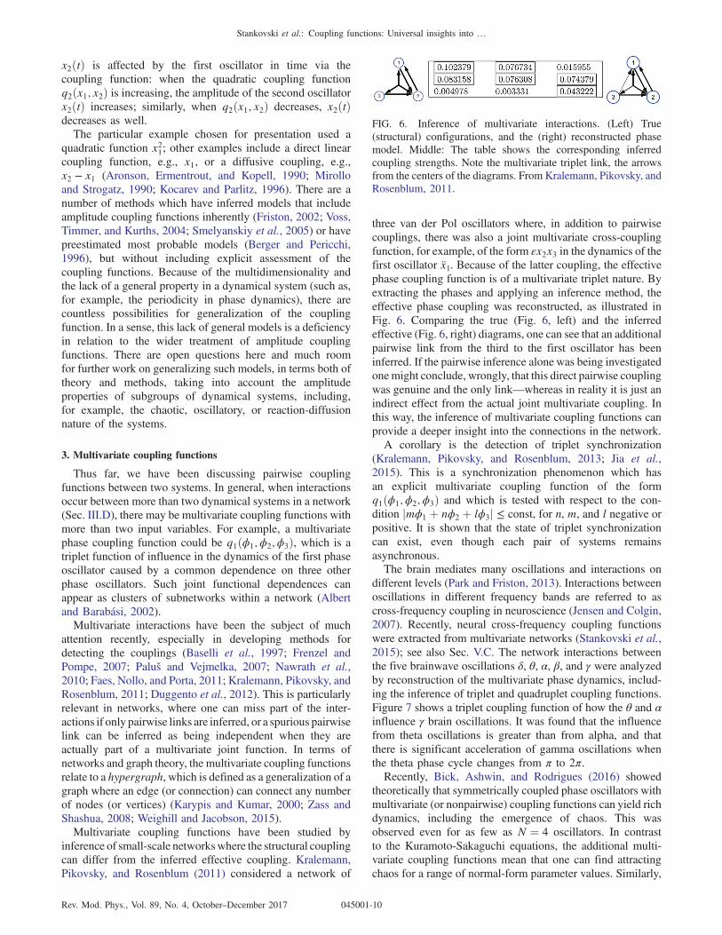
three van der Pol oscillators where, in addition to pairwisecouplings, there was also a joint multivariate cross-couplingfunction, for example, of the form εx2x3 in the dynamics of thefirst oscillator x1. Because of the latter coupling, the effectivephase coupling function is of a multivariate triplet nature. Byextracting the phases and applying an inference method, theeffective phase coupling was reconstructed, as illustrated inFig. 6. Comparing the true (Fig. 6, left) and the inferredeffective (Fig. 6, right) diagrams, one can see that an additionalpairwise link from the third to the first oscillator has beeninferred. If the pairwise inference alone was being investigatedonemight conclude, wrongly, that this direct pairwise couplingwas genuine and the only link—whereas in reality it is just anindirect effect from the actual joint multivariate coupling. Inthis way, the inference of multivariate coupling functions canprovide a deeper insight into the connections in the network.A corollary is the detection of triplet synchronization

(Kralemann, Pikovsky, and Rosenblum, 2013; Jia et al.,2015). This is a synchronization phenomenon which hasan explicit multivariate coupling function of the formq1ðϕ1;ϕ2;ϕ3Þ and which is tested with respect to the con-dition jmϕ1 þ nϕ2 þ lϕ3j ≤ const, for n, m, and l negative orpositive. It is shown that the state of triplet synchronizationcan exist, even though each pair of systems remainsasynchronous.The brain mediates many oscillations and interactions on

different levels (Park and Friston, 2013). Interactions betweenoscillations in different frequency bands are referred to ascross-frequency coupling in neuroscience (Jensen and Colgin,2007). Recently, neural cross-frequency coupling functionswere extracted from multivariate networks (Stankovski et al.,2015); see also Sec. V.C. The network interactions betweenthe five brainwave oscillations δ, θ, α, β, and γ were analyzedby reconstruction of the multivariate phase dynamics, includ-ing the inference of triplet and quadruplet coupling functions.Figure 7 shows a triplet coupling function of how the θ and αinfluence γ brain oscillations. It was found that the influencefrom theta oscillations is greater than from alpha, and thatthere is significant acceleration of gamma oscillations whenthe theta phase cycle changes from π to 2π.Recently, Bick, Ashwin, and Rodrigues (2016) showed

theoretically that symmetrically coupled phase oscillators withmultivariate (or nonpairwise) coupling functions can yield richdynamics, including the emergence of chaos. This wasobserved even for as few as N ¼ 4 oscillators. In contrastto the Kuramoto-Sakaguchi equations, the additional multi-variate coupling functions mean that one can find attractingchaos for a range of normal-form parameter values. Similarly,

FIG. 6. Inference of multivariate interactions. (Left) True(structural) configurations, and the (right) reconstructed phasemodel. Middle: The table shows the corresponding inferredcoupling strengths. Note the multivariate triplet link, the arrowsfrom the centers of the diagrams. From Kralemann, Pikovsky, andRosenblum, 2011.



it was found that even the standard Kuramoto model can bechaotic with a finite number of oscillators (Popovych,Maistrenko, and Tass, 2005).

4. Generality of coupling functions

The coupling function is well defined from a theoreticalperspective. That is, once we have the model [as in Eq. (1)],the coupling function is unique and fixed. The solutions of theequations also depend continuously on the coupling function.Small changes in the coupling function will cause only smallchanges in the solutions over finite-time intervals. If solutionsare attracted to some set exponentially and uniformly fast,then small changes in the coupling do not affect the stability ofthe system.When we want to infer the coupling function from data we

can face a number of challenges in obtaining a unique result(Sec. IV). Typically, we measure only projections of thecoupling function, which might in itself lead to nonuniquenessof the estimate. That is, we project the function (which isinfinite dimensional) onto a finite-dimensional vector space.In doing so, we could lose some information and, generically,it is not possible to uniquely estimate the function (evenwithout taking account of noise and perturbations).Furthermore, the final form of the estimated function dependson the choice and number of base functions. For example, thechoice of a Fourier series or general orthogonal polynomialsas base functions can slightly affect the final estimate of the

coupling function. The choice of which base functions to beused is infinite. Even though many aspects of couplingfunctions (such as the number of arguments, decompositionunder an appropriate model, analysis of coupling functioncomponents, prediction with coupling functions, etc.) can beapplied with great generality, the coupling functions them-selves cannot be uniquely determined.In the literature, authors often speak of the commonly used

coupling functions including, but not limited to, those listed inTable I. Note that reactive and diffusive couplings have func-tionally the same form, the difference being that the reactivecase includes complex amplitudes. This results in a phasedifference between the coupling and the dynamics. Also in theliterature, a diffusive coupling function qðy − xÞ satisfying alocal condition q0ð0Þ < 0 is called dissipative coupling(Rul’Kov et al., 1992). This condition resembles Fick’s lawas the coupling forces the coupled system to converge towardthe same state. When q0ð0Þ > 0 the coupling is called repulsive(Hens et al., 2013). Chemical synapses are an important form ofcoupling where the influences of x and y appear together as aproduct. There are also other interesting forms of coupling suchas the geometric mean and further generalizations (Prasad et al.,2010; Petereit and Pikovsky, 2017). In environmental coupling,the function is given by the solution of a differential equation. Inthis case one can consider _y ¼ −κyþ ε½xðtÞ þ yðtÞ& for κ > 0,so that the variables are considered as external fields driving theequation. Its solution yðtÞ ¼ yðt; x; yÞ is taken as the couplingfunction qðx; yÞ and, for t ≫ 1, is given in the table. Thegenerality of coupling functions, and the fact that the form cancome from an unbounded set of functions,was used to constructthe encryption key in a secure communications protocol(Stankovski,McClintock, andStefanovska, 2014); see Sec.V.F.

D. Coupling functions revealing mechanisms

The functional form is a qualitative property that definesthe mechanism and acts as an additional dimension tocomplement the quantitative characteristics such as the cou-pling strength, directionality, frequency parameter, and limit-cycle shape parameters. By definition, the mechanisminvolves some kind of function or process leading to a changein the affected system. Its significance is that it may lead toqualitative transitions and induce or reduce physical effects,including synchronization, instability, amplitude death, oroscillation death.But why is the mechanism important and how can it be

used? The first and foremost use of the coupling function

FIG. 7. Multivariate triplet coupling functions between neuraloscillations. The phase coupling function qγðϕθ;ϕαÞ shows theinfluence that θ and α jointly insert on the γ cortical oscillations.From Stankovski et al., 2015.

TABLE I. Different examples of coupling functions q. These pairwise coupling functions (CFs) are considered in relation to the system_x ¼ fðxÞ þ qðx; yÞ.

Type of CF Model Meaning Reference

Direct qðx; yÞ ¼ qðyÞ Unidirectional influence Aronson, Ermentrout, andKopell (1990)

Diffusive qðx; yÞ ¼ qðy − xÞ Dependence on state difference Kuramoto (1984)Reactive qðx; yÞ ¼ ðεþ iβÞqðx − yÞ Complex coupling strength Cross et al. (2006)Conjugate qðx; yÞ ¼ qðx − PyÞ P permutes the variables Karnatak, Ramaswamy, and

Prasad (2007)Chemical synapse qðx; yÞ ¼ gðxÞSðyÞ S is a sigmoidal Cosenza and Parravano (2001)Environmental qðx; yÞ ≈ ε

Rt0 e

−κðt−sÞ½xðsÞ þ yðsÞ&ds Given by a differential equation Resmi, Ambika, and Amritkar (2011)



mechanism is to illuminate the nature of the interactionsthemselves. For example, the coupling function of theBelousov-Zhabotinsky chemical oscillator was reconstructed(Miyazaki and Kinoshita, 2006) with the help of a method forthe inference of phase dynamics. Figure 8 shows such acoupling function, demonstrating a form that is very far from asinusoidal function: a curve that gradually decreases in theregion of a small ψ and abruptly increases at a larger ψ, withits minimum and maximum at around 5=4π and 7=4π,respectively.Another important set of examples is the class of coupling

functions and phase response curves used in neuroscience. Inneuronal interactions, some variables are very spikelike, i.e.,they resemble delta functions. Consequently, neuronal cou-pling functions (which are a convolution of phase responsecurves and perturbation functions) then depend only, ormainly, on the phase response curves. So the interactionmechanism is defined by the phase response curves: quitea lot of work has been done in this direction (Ermentrout,1996; Tateno and Robinson, 2007; Gouwens et al., 2010;Schultheiss, Prinz, and Butera, 2011); see also Sec. IV.D.2.For example, Tateno and Robinson (2007) and Gouwens et al.(2010) experimentally reconstructed the phase responsecurves for different types of interneurons in rat cortex, inorder to better understand the mechanisms of neuralsynchronization.The mechanism of a coupling function depends on the

differing contributions from individual oscillators. Changes inform may depend predominantly on only one of the phases(along one axis), or they may depend on both phases, oftenresulting in a complicated and intuitively unclear dependence.The mechanism specified by the form of the coupling functioncan be used to distinguish the individual functional contri-butions to a coupling. One can decompose the net couplingfunction into components describing the self-, direct, andindirect couplings (Iatsenko et al., 2013). The self-couplingdescribes the inner dynamics of an oscillator which resultsfrom the interactions and has little physical meaning. Directcoupling describes the influence of the direct (unidirectional)driving that one oscillator exerts on the other. The lastcomponent, indirect coupling, often called common coupling,depends on the shared contributions of the two oscillators,e.g., the diffusive coupling given with the phase difference

terms. This functional coupling decomposition can be furthergeneralized for multivariate coupling functions, where, forexample, a direct coupling from two oscillators to a third onecan be determined (Stankovski et al., 2015).After learning the details of the reconstructed coupling

function, one can use this knowledge to study or detect thephysical effects of the interactions. In this way, the synchro-nous behavior of the two coupled Belousov-Zhabotinskyreactors can be explained in terms of the coupling functionas illustrated by the examples given in Fig. 8 (Miyazaki andKinoshita, 2006) and Sec. V.A. Furthermore, the mechanismsand form of the coupling functions can be used to engineerand construct a particular complex dynamical structure,including sequential patterns and desynchronization ofelectrochemical oscillations (Kiss et al., 2007). Even moreimportantly, one can use knowledge about the mechanism ofthe reconstructed coupling function to predict transitions ofthe physical effects—an important property described in detailfor synchronization in the following section.

E. Synchronization prediction with coupling functions

Synchronization is a widespread phenomenon whoseoccurrence and disappearance can be of great importance.For example, epileptic seizures in the brain are associated withexcessive synchronization between a large number of neurons,so there is a need to control synchronization to provide ameans of stopping or preventing seizures (Schindler et al.,2007), while in power grids the maintenance of synchroniza-tion is of crucial importance (Rubido, 2015). Therefore, oneoften needs to be able to control and predict the onset anddisappearance of synchronization.A seminal work on coupling functions by Kiss, Zhai, and

Hudson (2005) uses the inferred knowledge of the couplingfunction to predict characteristic synchronization phenomenain electrochemical oscillators. In particular, they demonstratedthe power of phase coupling functions, obtained from directexperiments on a single oscillator, to predict the dependenceof synchronization characteristics such as order-disordertransitions on system parameters, both in small sets and inlarge populations of interacting electrochemical oscillators.They investigated the parametric dependence of mutual

entrainment using an electrochemical reaction system, theelectrodissolution of nickel in sulfuric acid (see also Sec. V.Afor further applications on chemical coupling functions).A single nickel electrodissolution oscillator can have twomain characteristic wave forms of periodic oscillation: thesmooth type and the relaxation oscillation type. The phaseresponse curve is of the smooth type and is nearly sinusoidal,while being more asymmetric for the relaxation oscillations.The coupling functions are calculated using the phase

response curve obtained from experimental data for thevariable through which the oscillators are coupled. Thecoupling functions qðψÞ of two coupled oscillators arereconstructed for three characteristic cases, as shown inFigs. 9(a)–9(c), left panels. The right panels in Fig. 9 showthe corresponding odd (antisymmetric) part of the couplingfunctions q−ðψÞ ¼ ½qðψÞ − qð−ψÞ&=2, which is important fordetermination of the synchronization. The coupling functionsqðψÞ of Figs. 9(a)–9(c) have predominantly positive values, so

FIG. 8. Coupling function determined from the phase dynamicsof two interacting chemical Belousov-Zhabotinsky oscillators.The coupling function is reconstructed in terms of the phasedifference ψ ¼ ϕ2 − ϕ1. Points obtained from reactors 1 and 2are plotted with open circles and triangles, respectively. The fullcurves represent smooth interpolations. From Miyazaki andKinoshita, 2006.



the interactions contribute to the acceleration of the affectedoscillators. The first coupling function of Fig. 9(a) for smoothoscillations has a sinusoidal q−ðψÞ which can lead to in-phasesynchronization at the phase difference of ψ' ¼ 0. The thirdcase of relaxation oscillations of Fig. 9(c) has an invertedsinusoidal form q−ðψÞ, leading to stable antiphase synchro-nization at ψ' ¼ π. The most peculiar case is Fig. 9(b), rightpanel, of relaxation oscillations, where the odd couplingfunction q−ðψÞ takes the form of a second harmonic[q−ðψÞ ≈ sinð2ψÞ] and both the in-phase (ψ' ¼ 0) and anti-phase (ψ' ¼ π) entrainments are stable, in which case theactual state attained will depend on the initial conditions.Next, the knowledge obtained from experiments with a

single oscillator was applied to predict the onset of synchro-nization in experiments with 64 globally coupled oscillators.The experiments confirmed that for smooth oscillators theinteractions converge to a single cluster, and for relaxationaloscillators they converge to a two-cluster synchronized state.Experiments in a parameter region between these states, inwhich bistability is predicted, are shown in Fig. 10. A smallperturbation of the stable one-cluster state (left panel ofFig. 10) yields a stable two-cluster state (right panel ofFig. 10). Therefore, all the synchronization behavior seenin the experiments was in agreement with prior predictionsbased on the coupling functions.In a separate line of work, synchronization was also

predicted in neuroscience: interaction mechanisms involvingindividual neurons, usually in terms of PRCs or spike-timeresponse curves, were used to understand and predict thesynchronous behavior of networks of neurons (Acker, Kopell,

and White, 2003; Netoff et al., 2005; Schultheiss, Prinz, andButera, 2011). For example, Netoff et al. (2005) experimen-tally studied the spike-time response curves of individualneuronal cells. Results from these single-cell experimentswere then used to predict the multicell network behaviors,which were found to be compatible with previous model-based predictions of how specific membrane mechanisms giverise to the empirically measured synchronization behavior.

F. Unifying nomenclature

Over the course of time, physicists have used a range ofdifferent terminology for coupling functions. For example,some publications refer to them as interaction functions andsome as coupling functions. This inconsistency needs to beovercome by adopting a common nomenclature for thefuture.The terms interaction function and coupling function have

both been used to describe the physical and mathematicallinks between interacting dynamical systems. Of these,coupling function has been used about twice as often in theliterature, including the most recent. The term coupling iscloser to describing a connection between two systems, whilethe term interaction is more general. Coupling impliescausality, whereas interaction does not necessarily do so.Often correlation and coherence are considered as signaturesof interactions, while they do not necessarily imply theexistence of couplings. We therefore propose that the termi-nology be unified, and the term coupling function be usedhenceforth to characterize the link between two dynamicalsystems whose interaction is also causal.

III. THEORY

In physics one is likely to examine stable static configu-rations, whereas, in dynamical interaction between oscillators,solutions will converge to a subspace. For example, if twooscillators are in complete synchronization the subspace iscalled the synchronization manifold and corresponds to thecase where the oscillators are in the same state for all time(Fujisaka and Yamada, 1983; Pecora and Carroll, 1990).

FIG. 9. Experimental coupling function from electrochemicaloscillators used for the prediction of synchronization.(a)–(c) Coupling function qðψÞ evaluated with respect to thephase difference ψ ¼ ϕ2 − ϕ1 shown in the left panel and its oddpart q−ðΔϕÞ shown in the right panel—for the case of (a) asmooth oscillator, and (b), (c) for relaxation oscillators withslightly different parameters. HðΔϕÞ on the plots is equivalent tothe qðψÞ notation used in the current review. From Kiss, Zhai, andHudson, 2005.

FIG. 10. Mutual entrainment and stable (left panel) single-cluster and (right panel) two-cluster states of a population of64 globally coupled electrochemical relaxation oscillatorsunder the same experimental conditions. The two-cluster statewas obtained from the one-cluster state by a small perturbationacting as a different initial condition for the population. FromKiss, Zhai, and Hudson, 2005.



So, within the subspace, the oscillators have their owndynamics and finer information on the coupling function isneeded.The analytical techniques and methods needed to analyze

the dynamics will depend on whether the coupling strength isstrong or weak. Roughly speaking, in the strong couplingregime, we have to tackle the fully coupled oscillators whereasin the weak coupling we can reduce the analysis to lower-dimensional equations.

A. Strong interaction

To illustrate the main ideas and challenges of treating thecase of strong interaction, while keeping technicalities to aminimum, we first discuss the case of two coupled oscillators.These examples contain the main ideas and reveal the role ofthe coupling function and how it guides the system towardsynchronization.

1. Two coupled oscillators

We start by illustrating the variety of dynamical phenomenathat can be encountered and the role played by the couplingfunction in the strong coupling regime.Diffusion-driven oscillations.—When two systems interact

they may display oscillations solely because of the interaction.This is the nature of the problem posed by Smale (1976) basedon Turing’s idea of morphogenesis (Turing, 1952). Weconsider two identical systems which, when isolated, eachexhibit a globally asymptotically stable equilibrium, butwhich oscillate when diffusively coupled. This phenomenonis called diffusion-driven oscillation.Assume that the system

_x ¼ fðxÞ; ð12Þ

where f∶ Rn → Rn is a differentiable vector field with aglobally stable attraction with point—all trajectories willconverge to this point. Now consider two of such systemscoupled diffusively

_x1 ¼ fðx1Þ þ εHðx2 − x1Þ;_x2 ¼ fðx2Þ þ εHðx1 − x2Þ: ð13Þ

The problem proposed by Smale was to find (if possible) acoupling function (positive definite matrix) H such that thediffusively coupled system undergoes a Hopf bifurcation.Loosely speaking, one may think of two cells that bythemselves are inert but which, when they interact diffusively,become alive in a dynamical sense and start to oscillate.Interestingly, the dimension of the uncoupled systems

comes into play. Smale constructed an example in fourdimensions. Pogromsky, Glad, and Nijmeijer (1999) con-structed examples in three dimensions and also showed that,under suitable conditions, the minimum dimension for dif-fusive coupling to result in oscillation is n ¼ 3. The followingexample illustrates the main ideas. Consider

fðxÞ ¼ Axð1þ jxj2Þ with A ¼

0

B@1 −1 1

1 0 0

−4 2 −3

1

CA; ð14Þ

where jxj2 ¼ xTx. Note that all the eigenvalues of A havenegative real parts. So the origin of the system Eq. (14) isexponentially attracting.Consider the coupling function to be the identity

_x1 ¼ fðx1Þ þ εðx2 − x1Þ;_x2 ¼ fðx2Þ þ εðx1 − x2Þ:

For ε ¼ 0 the origin is globally attracting; the uniformattraction persists when ε is very small, and so the origin isstill globally attracting. However, for large values of thecoupling ε > 0.6512 the coupled systems exhibit oscillatorysolutions (the origin has undergone a Hopf bifurcation).Generalizations.—In this example the coupling function

was the identity. Pogromsky, Glad, and Nijmeijer (1999)discussed further coupling functions, such as coupling func-tions of rank two that generate diffusion-driven oscillators.Further oscillations in originally passive systems have beenreported in spatially extended systems (Gomez-Marin, Garcia-Ojalvo, and Sancho, 2007). In diffusively coupled mem-branes, collective oscillation in a group of nonoscillatorycells can also occur as a result of a spatially inhomogeneousactivation factor (Ma and Yoshikawa, 2009). These ideas ofdiffusion leading to chemical differentiation have also beenobserved experimentally and generalized by including hetero-geneity in the model (Tompkins et al., 2014).Oscillation death.—We now consider the opposite prob-

lem: Systems which when isolated exhibit oscillatory behaviorbut which, when coupled diffusively, cease to oscillate andwhere the solutions converge to an equilibrium point.As mentioned in Sec. I.B, this phenomenon is called

oscillation death (Bar-Eli, 1985; Ermentrout and Kopell,1990; Mirollo and Strogatz, 1990; Koseska, Volkov, andKurths, 2013a). To illustrate the essential features we considera normal form of the Hopf bifurcation

_xj ¼ fjðxjÞ;

where

fjðxÞ ¼ ωjAxþ ð1 − jxj2Þx; with A ¼$0 −11 0

%:

So each isolated system has a limit cycle of amplitude jxj2 ¼ 1and a frequency ωj. Note that the origin x ¼ 0 is an unstableequilibrium point. In oscillation death when the systems arecoupled, the origin may become stable.Focusing on diffusive coupling, again the question concerns

the nature of the coupling function. Aronson, Ermentrout, andKopell (1990) remarked that the simplest coupling function tohave the desired properties is the identity with strength ε. Theequations have the same form as Eq. (13) with H being theidentity.



The effect can be better understood in terms of phase andamplitude variables. Let r1 and r2 be the amplitudes and ϕ1

and ϕ2 the phases of x1 and x2, respectively. We considerr1 ¼ r2 ¼ r which captures the main causes of the effect, aswell as the phase difference ψ ¼ ϕ1 − ϕ2. Then the equationsin these variables can be well approximated as

_r ¼ rð1 − ε − r2Þ þ εr cosψ ; ð15Þ

_ψ ¼ Δω − 2ε sinψ : ð16Þ

The conditions for oscillation death are a stable fixed point atr ¼ 0 along with a stable fixed point for the phase dynamics.These equations provide the main mechanism for oscillationdeath. First, we can determine the stable fixed point for thephase dynamics, as illustrated in Fig. 2. There is a fixed pointψ' if ε>Δω=2 and sinψ' ¼ Δω=ð2εÞ. We assume thatΔω > 2which implies that, when the fixed point ψ' exists, ε > 1.Next, we analyze the stability of the fixed point r' ¼ 0.

This is determined by the linear part of Eq. (15). Hence, thecondition for stability is

1 − εþ ε cosψ' < 0:

Using the equation for the fixed point we have cosψ' ¼ffiffiffiffiffiffiffiffiffiffiffiffiffiffiffiffiffiffiffiffiffiffiffiffiffiffiffiffiffi1 − ½Δω=ð2εÞ&2

p. Replacing this in the stability condition we

obtain ε < ð4þ Δ2ωÞ=8. The analysis reveals that the system

will exhibit oscillation death if the coupling is neither tooweak nor too strong. Because we are assuming that themismatch is large enough, Δω > 2, then there are minimumand maximum coupling strengths for oscillation death

1 < ε <4þ Δ2

ω

4:

Within this range, there are no stable limit cycles: the onlyattracting point is the origin, and so the oscillations are dead.The full equation was tackled by Aronson, Ermentrout, and

Kopell (1990). The main principle is that the eigenvalues ofthe coupling function modify the original eigenvalues of thesystem and change their stability. It is possible to generalizethese claims to coupling functions that are far from the identity(Koseska, Volkov, and Kurths, 2013a). The system mayconverge, not only to a single fixed point, but to many(Koseska, Volkov, and Kurths, 2013b).Synchronization.—One of the main roles of coupling

functions is to facilitate collective dynamics. Consider thediffusively coupled oscillators described by Eq. (13). We saythat the diagonal

x1ðtÞ ¼ x2ðtÞ

is the complete synchronization manifold (Brown andKocarev, 2000). Note that the synchronization manifold isan invariant subspace of the equations of motion for all valuesof the coupling strength. Indeed, when the oscillators syn-chronize the coupling term vanishes. So they will besynchronized for all future time. The main question is whetherthe synchronization manifold is attractive; that is, if theoscillators are not precisely synchronized will they converge

toward synchronization? Similarly, if they are synchronized,and one perturbs the synchronization, will they return tosynchronization?Let us first consider the case where the coupling is the

identity HðxÞ ¼ x and discuss the key mechanism for syn-chronization. Note that there are natural coordinates to analyzesynchronization

y ¼ 12ðx1 þ x2Þ and z ¼ 1

2ðx1 − x2Þ:

These coordinates have a natural meaning. If the systemsynchronizes, z → 0 and y → s with _s ¼ fðsÞ. Hence, werefer to y as the coordinate parallel to the synchronizationsubspace x1 ¼ x2, and to z as the coordinate transverse to thesynchronization subspace, as illustrated in Fig. 11.The synchronization analysis follows two steps:

(i) Obtaining a governing equation for the modes z transverseto the synchronization subspace, and (ii) using the couplingfunction to damp instabilities in the transverse modes.

(i) Obtain an equation for z.—Let us assume that theinitial disturbance of z is small. Then we can obtaina linear equation for z by neglecting the highorder terms proportional to jzj2. Noting that _z ¼ð _x1 − _x2Þ=2, using Eqs. (13) for x1 and x2, andexpanding f in a Taylor series, we obtain

_z ¼ JðtÞz − 2εz; ð17Þ

where JðtÞ ¼ Df(x2ðtÞ) is the Jacobian evaluatedalong a solution of x2.

(ii) Coupling function to provide damping.—The term−2εz coming from the coupling now plays the roleof a damping term. So we expect that the couplingwill win the competition with J and will force thesolutions of z to decay exponentially fast to zero. Tosee this, we observe that the first term

_u ¼ JðtÞu ð18Þ

depends on the dynamics of x2 alone. Typically,kuðtÞk ∝ eλt for λ > 0. Now, to obtain a bound on

FIG. 11. Illustration of the coordinates parallel y and transversez to synchronization. In the left panel we also show a trajectoryconverging to the synchronization subspace implying that z → 0.Once the coupled systems reach synchronization, their ampli-tudes will evolve together in time, but the evolution can bechaotic as illustrated in the right panel. The dynamics along thesynchronization subspace is the Lorenz attractor.



the solution of Eq. (17), we consider the ansatzz ¼ ue−2εt, and notice that differentiating z weobtain Eq. (17). Hence

kzðtÞk ∝ eðλ−2εÞt;

from the growth behavior of the disturbance z wecan also obtain the critical coupling strength toobserve synchronization.

Critical coupling.—From this estimate, we can also obtainthe critical coupling such that the solutions z decay to zero.For coupling strengths

ε >λ2;

the oscillators synchronize.Meaning of λ > 0.—This corresponds to chaotic behavior

in the synchronization manifold. If z → 0, then JðtÞ will bethe Jacobian along a solution of _s ¼ fðsÞ. So λ depends on thedynamics on the synchronization manifold. If λ > 0 and thesolutions are bounded, the dynamics of the synchronizedsystem is chaotic. Roughly speaking, λ > 0 means that twonearby trajectories will diverge exponentially fast for smalltimes and, because the solutions are bounded, they willsubsequently come close together again. So the coupledsystems can synchronize even if the dynamics of thesynchronized system is chaotic, as shown in Fig. 11 for thechaotic Lorenz attractor. The number λ is the maximumLyapunov exponent of the synchronization subspace.There are intrinsic challenges associated with the analysis

and more when we attempt to generalize these ideas and alsobecause of the nonlinearities that we neglected during theanalysis.

(1) General coupling functions: From a mathematicalperspective the argument above worked because theidentity commutes with all matrices. For other cou-pling functions, the argument above cannot be applied,and we encounter three possible scenarios.(i) The coupling function does not damp instabil-

ities and the system never synchronizes (Pecoraand Carroll, 1998; Boccaletti et al., 2002).

(ii) The coupling function damps out instabilitiesonly for a finite range of coupling strengths,

ε1c < ε < ε2c:

For instance, this is the case for the Rösslersystem with coupling only in the first variable(Huang et al., 2009).

(iii) The coupling function damps instabilities andthere is a single critical coupling εc. This is thecase when the coupling function eigenvalueshave positive real parts. (Pereira et al., 2014).

(2) Local versus global results: In this argument weexpanded the vector field in a Taylor series andobtained a linear equation to describe how the systemssynchronize. This means that any claim on synchro-nization is local. It is still an open question how toobtain global results.

(3) Nonlinear effects: We neglected the nonlinear terms(the Taylor remainders), which can make synchroni-zation unstable. Many researchers have observed thisphenomenon through the bubbling transition (Ashwin,Buescu, and Stewart, 1994; Venkataramani et al.,1996; Viana et al., 2005), intermittent loss of syn-chronization (Gauthier and Bienfang, 1996; Yanchuk,Maistrenko, and Mosekilde, 2001), and the riddlingbasin (Heagy, Carroll, and Pecora, 1994; Ashwin andTimme, 2005).

To highlight the role of the coupling function and illustratethe challenges, we show how to obtain global results depend-ing on the coupling function and discuss how local and globalresults are related.Global argument.—Assume that H is a Hermitian positive

definite matrix. The main idea is to turn the problem upsidedown. That is, we see the vector field as perturbing thecoupling function. So consider the system with only thecoupling function and use the transverse coordinates

_z ¼ −2εHz: ð19Þ

Since H is positive definite we obtain −zTHz ≤ −2cεjzj2,where c ¼ cðHÞ is the smallest eigenvalue of H. The globalstability of the system can be obtained by constructing aLyapunov function (LF) V. The system will be stable if V ispositive and its derivative _V is negative. This system admits aquadratic Lyapunov function VðzÞ ¼ 1

2 zTz. Indeed, taking the

derivative

_VðzÞ ¼ zT _z ≤ −2cεjzj2:

Hence all solutions of Eq. (19) will converge to zeroexponentially fast. Next consider the coupled system

_z ¼ −2εHzþ Jðt; zÞ;

where by the mean value theorem we obtain

Jðt; zÞ ¼ f(x1ðtÞ þ zðtÞ) − fðx1ðtÞÞ

¼Z

1

0Df(x1ðtÞ þ szðtÞ)zðtÞds: ð20Þ

Because we did not Taylor expand the vector fields, theequation is globally valid. Assuming that the Jacobian isbounded by a constant Mf > 0, we obtain jJðt; zÞj ≤ Mfjzj.Computing again the Lyapunov function for the coupled

system (including the vector fields) we obtain

_VðzÞ ≤ −ð2cε −MfÞjzj2: ð21Þ

The system will synchronize if _V is negative. So synchroni-zation is attained if

εc >Mf

2c:

Again the critical coupling has the same form as before. Thecoupling function came into play via the constant c, and



instead of λ we have Mf. Typically,Mf is much larger than λ.So global bounds are not sharp. This conservative boundguarantees that the coupling function can damp all possibleinstabilities transverse to the synchronization manifold.Moreover, they are persistent under perturbation.Local results.—First we Taylor expand the system to obtain

_z ¼ JðtÞz − 2εHz ð22Þ

in just the same form as before. Note, however, that the trickwe used previously, by defining _u ¼ Ju, is no longerapplicable. Indeed we use the ansatz z ¼ ue−2εHt to obtain_z ¼ −2εHzþ e−2εHtJðtÞu, and since H and JðtÞ do notcommute,

e−2εHtJðtÞu ≠ JðtÞe−2εHtu ¼ JðtÞz;

the ansatz cannot be used. Thus we need a better way forward.So in the same way as we calculated the expansion rate λ forJðtÞ, we calculate the expansion rate for Eq. (22). SuchLyapunov exponents are important in a variety of contexts. Forus, it suffices to know that there are various ways to computethem (Dieci and Van Vleck, 2002; Pikovsky and Politi, 2016).We calculate the Lyapunov exponent for each value of thecoupling strength ε to obtain a function

ε ↦ ΛðεÞ:

This function is called the master stability function (MSF).We extract the synchronization properties from ΛðεÞ. Asdiscussed, the solutions of Eq. (19) will behave as

jzðtÞj ∝ CeΛðεÞt:

Now note that Λð0Þ ¼ λ > 0 (the expansion rate of theuncoupled equation), since we considered the case of chaoticoscillators. Because of our assumptions, we know that there isa εc such that

ε > εMSFc ⇒ ΛðεÞ < 0

and for which ΛðεÞ will become negative, and z will convergeto zero.Global versus local results.—In the global analysis, the

critical coupling depends on Mf, which is an upper bound forthe Jacobian. This approach is rigorous and guarantees that allsolutions will synchronize. In the local analysis, we linearizedthe dynamics about the synchronization manifold and com-puted the Lyapunov exponent associated with the transversecoordinate z. The critical coupling was then obtained byanalyzing the sign of the Lyapunov exponent. Generically,εMSFc ≪ Mf=2c. The main reasoning is as follows. TheLyapunov exponents measure the mean instability, whereas,in the global argument, we consider the worst possibleinstability. So the local method allows us to obtain a sharpestimate for the onset of synchronization.The pitfalls of the local results.—The main challenge of the

local method lies in the intricacies of the theory of Lyapunovexponents (Barreira and Pesin, 2002; Pikovsky and Politi,

2016). These can be discontinuous functions of the vectorfield. In other words, the nonlinear terms we threw away asTaylor remainders can make the Lyapunov exponent jumpfrom negative to positive. Moreover, in the local case wecannot guarantee that all trajectories will be uniformlyattracted to the synchronization manifold. In fact, for someinitial conditions trajectories are attracted to the synchroniza-tion manifold, whereas nearby initial conditions are not.This phenomenon is called riddling (Heagy, Carroll, andPecora, 1994).

2. Comparison between approaches

As previously discussed, there is a dichotomy betweenglobal versus local results and sharp bounds for criticalcoupling. These issues depend on the coupling function.Some coupling functions allow one to employ a giventechnique and thereby obtain global or local results.First we compare the two main techniques used in the

literature, that is, Lyapunov functions and the master stabilityfunction. For a generic coupling function, the LFs areunknown, but Lyapunov exponents can be estimated effi-ciently by numerical methods (Dieci and Van Vleck, 2002;Ginelli et al., 2007; Froyland et al., 2013).Given additional information on the coupling, we can

further compare the techniques. Note that the couplingfunction H can be nonlinear. In this case, we consider theJacobian

Γ ¼ DHð0Þ:

Moreover, we say that Γ belongs to the Lyapunov class if thereare positive matrices Q and P such that

ΓTPþ PΓ ¼ −Q:

Whenever the matrix Γ is in the Lyapunov class we canconstruct the Lyapunov function algorithmically.Table II reveals that the MSF method is very versatile.

Although it may not encompass nonlinear perturbations, itprovides a framework to tackle a generic class of couplingfunctions (Huang et al., 2009). In the theory of chaoticsynchronization, therefore, this has been the preferredapproach. However, it should be used with caution.

B. Weak regime

In the weak coupling regime, the coupling strength is bydefinition insufficient to significantly affect the amplitudes;

TABLE II. Comparison between classes of coupling function andthe techniques to obtain synchronization. Dashes indicate thattypically we are unable to construct the Lyapunov function in suchcases.

Coupling function Class Technique Global Persistence

H þve definite Lyapunov LF Yes YesDH þve definite Lyapunov LF No YesH differentiable Generic LF — —H differentiable Generic MSF No No



however, the coupling can still cause the phases to adapt andadjust their dynamics (Kuramoto, 1984). Many of the phe-nomena observed in nature relate to the weak coupling regime.Mathematical descriptions of coupled oscillators in

terms of their phases offer two advantages: first, it reducesthe dimension of the problem, and secondly, it can revealprinciples of collective dynamics and other phenomena.The theory for the weak coupling regime is well developed.

In the 1970s and early 1980s Winfree (1967, 1980) andKuramoto (1975, 1984) developed the idea of asymptoticphase and phase reduction. Also starting from the 1970s, themathematical theory for such phase reduction was brought tocompletion in terms of normally hyperbolic invariantmanifolds (Hirsch, Shub, and Pugh, 1977; Eldering, 2013;Wiggins, 2013). Since then, the phase reduction theory(Nakao, 2015) has been significantly extended and general-ized, for inclusion of phase reduction in the case of stronglyperturbed oscillations, for stochastic treatment of interactingoscillators subject to noise of different kinds, for oscillatingneuronal populations, and for spatiotemporal oscillations inreaction-diffusion systems (Brown, Moehlis, and Holmes,2004; Yoshimura and Arai, 2008; Teramae, Nakao, andErmentrout, 2009; Goldobin et al., 2010; Kurebayashi,Shirasaka, and Nakao, 2013; Nakao, Yanagita, andKawamura, 2014). The main ingredient in this approach isan attracting periodic orbit.

1. Stable periodic orbit and its phase

If the system in question has an exponentially stableperiodic orbit, the theory guarantees the existence of thereduction and provides a method to obtain it. Thanks toErmentrout (1996), Rinzel and Ermentrout (1998), Izhikevich(2007), Ermentrout, Galán, and Urban (2008), Ermentrout andTerman (2010), and Hoppensteadt and Izhikevich (2012) wenow have a phase description for certain classes of neuronsand we understand its limitations (Smeal, Ermentrout, andWhite, 2010). The strategy is as follows. We assume that thesystem

_x ¼ fðxÞ; ð23Þ

where f∶ Rn → Rn, has a uniformly exponentially attractingperiodic orbit γ with period T; that is, γðtþ TÞ ¼ γðtÞ. Theorbit is exponentially stable if the trajectories of the systemapproach it exponentially fast and the rate of convergencedoes not depend on the initial time or on initial conditions (forpoints sufficiently close to the orbit).We can parametrize the orbit by its phase ϕ,

γðϕþ 2πÞ ¼ γðϕÞ. We can also reparametrize time such thatthe phase ϕ increases uniformly along the orbit γ. That is, thephase is uniform frequency equal to unity. By the chain rulewe then have

_ϕ ¼ 1 ¼ ∇γϕ · fðγÞ.

The key idea here is that weak coupling can adjust the rhythmof the phase dynamics. The goal is to obtain the phasereduction solely on the basis of information about the isolatedsystem (the orbit γ). To this end we need to extend the phase φ

to a neighborhood of the orbit. The main ingredient necessaryfor the reduction of the problem to its phase dynamics is theconcept of asymptotic phase (Winfree, 1967, 1980), whichwill provide us with the coupling function.Asymptotic phase.—Right now, the phase ϕ is defined only

along the orbit γ. Our first step is to extend ϕ to a neighbor-hood of γ. Since the periodic orbit is exponentially anduniformly attracting, it will attract an open neighborhood ofγ. We call this set the basin of attraction of the periodic orbit.Note that every initial point x0 in the basin of attraction ofthe orbit will converge to the orbit. Hence, we have a ϕðx0Þsuch that

limt→∞

jxðt; x0Þ − γ(tþ ϕðx0Þ)j ¼ 0;

where xðt; x0Þ is the solution of the system with initialcondition x0. For each initial point in the basin of attractionof γ we can assign a unique point in the orbit θ. Thisϕ ∈ ½0; 2π& is called the asymptotic phase.Isochron.—For each value of phase ϕ in the orbit γ we have

a curve passing through this phase value. And along this curveevery initial will have the same asymptotic phase. This set iscalled an isochron. That is, the isochron is a level set of ϕðxÞ.So points in the isochron have the same value of phase andwill move at the same speed. See Fig. 12 where points in the

FIG. 12. Periodic orbits are shown as solid (black) circles andisochrons as (blue) lines. Every point in an isochron has the samevalue of asymptotic phase. Moreover, the distance between twopoints in the same isochron tends to zero exponentially fast, asillustrated by the red (dark) and blue (light) points. In the lowerfigure, we show the effect on the phase dynamics of a smallperturbation. The point is initially at phase zero. The perturbationΔx moves the system from its initial point to another isochron,thereby advancing the phase. The periodic orbit γ and theisochrons are for Eq. (25).



same isochron approach the orbit along the same isochron.The set of points where the isochron cannot be defined iscalled phaseless. Once we find the isochron we can performthe phase reduction.

2. Coupling function and phase reduction

Consider Eq. (23) with a stable periodic orbit γ beingperturbed

_x ¼ fðxÞ þ εIðϑ; xÞ;

where ϑ ¼ ωt is the phase of the external influence, and I isthe influence is a periodic on ϑ. The weak coupling impliesε ≪ 1.One of the cornerstones of the theory of invariant manifolds

is to guarantee that, when the system is perturbed and thecoupling strength is weak ε ≪ 1, there is a new attractingperiodic orbit ~γ close to the orbit γ, the difference between theorbits being of the order of ε. Moreover, ~γ is exponentiallyattractive and the isochrons also persist. So, while theamplitudes are basically unaffected, the dynamics of thephases change greatly.With the help of the asymptotic phase, we define the phase

in a neighborhood of the orbit γ. This neighborhood containsthe new orbit ~γ as we consider small ε > 0. So, calculating thephase along ~γ, by the chain rule we obtain

_ϕ ¼ ∇~γϕ · ½fð~γÞ þ εIðϑ; ~γÞ&:

But by construction ∇ϕ · f ¼ 1 in a neighborhood of γ.Because ~γ is OðεÞ distant from γ we can expand both f andI and evaluate them along γ at the expense of a perturbation ofthe order of ε. It is standard to denote Z ¼ ∇γϕ. In this settingwe have

_ϕ ¼ 1þ εZðϕÞ · I(ϑ; γðϕÞ)þOðε2Þ;

and we have successfully reduced the problem to the phase ofthe unperturbed orbit γ. In general terms, we study problemsof the type

_ϕ ¼ 1þ εqðϕ; ϑÞ: ð24Þ

The main insight was to obtain the coupling function in termsof how the phase of the unperturbed orbit behaves near theorbit γ. We performed the following steps:

(1) Phase sensitivity Z of the unperturbed system.—Oncewe have the asymptotic phase, we can use it as the newphase variable ϕ, extending the definition of phasealong the orbit to a neighborhood of the orbit. Fromthe phase, we can in turn compute the phase sensitivityfunction

Z ¼ ∇ϕ;

where the gradient is evaluated along the orbit γ.(2) Obtain the coupling function by q ¼ Z · I.—For this

step, we need to take the inner product of Z with theperturbation p. When studying collective phenomena,

q will contain fast and slow variables. Typically, onlythe slow variables are of interest, so we average q overthe fast variables.

Meaning of q.—In this approach we have a strongunderlying assumption that the phase responds linearly toperturbations. That is, the coupling function is linear in theperturbations. If the phase is perturbed by I1 and I2, the neteffect will be the sum of I1 and I2. Notice that the linearity isonly in terms of the perturbations. The equation itself isnonlinear in the phase variable φ. The linearity with respect toperturbations is because we have discarded all nonlinear termsand terms of the order of ε2 (by computing Z along theunperturbed orbit). We discuss these issues in an examplelater. This linearity will facilitate the study of networks andlarge ensembles of oscillators.These two steps provide the phase description for weakly

coupled oscillators. Using these steps, it is possible to explainthe collective behavior of neurons (Ermentrout, 1996) andcircadian dynamics (Winfree, 1980), among other processes(Kuramoto, 1984; Ermentrout and Terman, 2010).

3. Synchronization with external forcing

We illustrate and discuss how these ideas can be applied tostudy the problem of synchronization with external forcing.Consider the system

_x ¼ fðxÞ ¼ xþ jxj2Ax; with A ¼$1 −11 1

%: ð25Þ

By inspection, it is clear that x ¼ 0 is an unstable point and thesystem has an attracting periodic orbit γ of radius 1. This canbe better seen by changing to polar coordinates x1ðr;ϕÞ ¼r sinðφÞ and x2ðr;φÞ ¼ r cosðφÞ using

_r ¼ rð1 − r2Þ; _φ ¼ r2: ð26Þ

The orbit γ corresponds to r ¼ 1 and is shown in Fig. 12.Asymptotic phase.—The phase φ as defined in the orbit γ

has a constant frequency equal to unity. Along the orbit γ, wetherefore have _φ ¼ 1 (by inspection of the equations). Forpoints outside the orbit, however, this is no longer true. Theasymptotic phase ϕ will fix this issue because the points thenmove at the same speed as the corresponding points in theorbit, so that _ϕ ¼ 1 for points outside the orbit.Because of the symmetry (r does not depend on φ) we can

use the ansatz

ϕðr;φÞ ¼ φþ ζðrÞ;

where we aim to find the function ζ. Differentiating we obtain

_ϕ ¼ _φþ dζdr

drdt

and, using the isochron’s properties together with the equa-tions for r and φ, we obtain _ζ ¼ 1=r so ζ ¼ log rþ C. Sincewe want to extend the phase continuously from the orbit, ifx ∈ γ then ϕðxÞ ¼ φðxÞ. We choose the constant C ¼ 0.Therefore,



ϕðr;φÞ ¼ φþ log r;

and we can define the isochron with asymptotic phaseϕðr;φÞ ¼ c. In Fig. 12 (top) we show four level sets of theasymptotic phase corresponding to ϕ ¼ 0, π=2, π, and 3π=2.We can use the asymptotic phase to obtain a coordinate that

decouples the phase dynamics from the other coordinates.Note that by defining a new coordinate ϕ ¼ φ − ηðrÞ weobtain

_ϕ ¼ ∇ϕ · f ¼ 1; ð27Þ

which is valid not only along the orbit γ via Eq. (26), but alsoin a neighborhood of the orbit. In the first equality we juststressed the identity between the frequency (applying thechain rule) and the gradient of ϕ.We can now readily take the gradient (in polar coordinates),

yielding ∇ϕ¼ e1½sinðϕ− logðrÞ&þ cos½ϕ− logðrÞ&=r. Alongthe unperturbed orbit γ we have ZðϕÞ ¼ ∇γϕ so that thephase sensitivity functions are

ZðϕÞ ¼ e1 sinðϕþ π=4Þ:

Next we obtain the coupling function.Obtaining the coupling function of external forcing.—Now

we consider the system being forced at frequency

_x ¼ fðxÞ þ εIðϑÞ; ð28Þ

where ϑ ¼ ωt. We obtain the coupling function through theisochron. We now justify in detail why we discarded thecorrections in ε2.We compute the equation for the phase dynamics. Note that

by chain rule _ϕ ¼ ∇ϕ · _x ¼ ∇ϕ · ½fðxÞ þ εI&. Using Eq. (27)and evaluating the gradient along the orbit ~γ, we obtain

_ϕ ¼ 1þ ε∇~γϕ · I:

For small ε, we know that the difference between ∇γϕ and∇~γϕ is of the order of ε, so we can replace the gradient alongthe perturbed orbit and unperturbed orbit with corrections ofthe order of ε2 (because ε is already multiplying the function).Hence,

_ϕ ¼ 1þ εqðϕ; ϑÞ þOðε2Þ:

Synchronization and coupling function.—The main idea isthat the coupling function q can help in adjusting thefrequency of the system to the frequency ω of the forcing.As discussed, we neglect the terms Oðε2Þ. Introducing thephase difference

ψ ¼ ϕ − ϑ

and considering 1 − ω ¼ Δω we obtain

_ψ ¼ Δω þ εZðψ þ ϑÞ · IðϑÞ:

IfΔω is of the order of ε then the dynamics of ψ will be slow incomparison with the dynamics of θ. Roughly speaking, foreach cycle of ψ we have 1=ε cycles of θ. Because the

dynamics of ϑ is faster than that of ψ , we use the averagingmethod to obtain the coupling function

qðψÞ ¼ 1

T

ZT

0Zðψ þ ϑÞ · IðϑÞdϑ;

where T ¼ 2π is the period of p as a function of ϑ. Note thatfor our result Z is sinusoidal so that by integrating over ϑwhile keeping ψ fixed, we obtain qðψÞ ¼ A sinðψ þ βÞ.Hence we obtain the dynamics in terms of the phase difference

dψdt

¼ Δω þ εqðψÞ; ð29Þ

which is exactly the equation shown in Fig. 2.We are now ready to study collective phenomena between

the driving and the system. For instance, the system will phaselock with the driving dynamics when Δþ εqðψ'Þ ¼ 0. In thiscase, the oscillators will have the same frequency. Moreover,because q is a periodic function, the fixed point ψ' will existonly when jΔ=εj ≤ max q.Higher-order n:m phase locking.—Our assumption is that

Δ ¼ OðεÞ, so that Eq. (29) for the phase difference ψ ¼ ϕ − ϑis a slow variable. It may happen that ψmn ¼ mφ − nϑ givesrise to a slow variable. In such cases, we perform the sameanalysis for ψmn and further information on the higher-orderphase locking can be obtained (Ermentrout, 1981).

4. Phase response curve

The phase sensitivity function Z plays a major role in thisanalysis. It also has many names: infinitesimal phase responsecurve (iPRC), linear response function, or infinitesimal phaseresetting curve. It is deeply related to the PRC. For anoscillator to be able to adjust its rhythm and synchronize, itmust respond differently to the perturbations at differentphases ϕ. So the phase can advance or retard to adjust itsrhythm to the external forcing. The PRC is a natural way ofdisplaying the response of oscillators to perturbations andthereby to gain insight into the collective dynamics.The main idea of the PRC is as follows: If we perform a

small and short perturbation of the orbit, the phase maycomplete its cycle before expectation (in the absence ofperturbations), or it may be delayed. The unperturbed periodof the orbit γ is T0. Every point on the orbit can be uniquelydescribed by the phase ϕ. A small perturbation applied at aphase ϕs can cause the phase to complete its full cycle at timeT1. The normalized phase difference between the cycles is

PRC ¼ T0 − T1

T0

:

Note that the PRC depends on the phase ϕs at which the smallperturbation was applied; that is, PRC ¼ PRCðϕsÞ. This is theso-called phase response curve.In the theory of weakly coupled oscillators, we use

the concept of an iPRC. It is equivalent to the gradient ofthe phase Z, and it is defined as the PRC normalized by theamplitude of the perturbation A:

Z ¼ limA→0

PRCA

:



Indeed, the isochrons and the PRC are closely related. If apoint moving along the orbit γ is instantaneous and theperturbation is small, the point will land on an isochron,which tells us the new phase ϕ of the point once it comes backto the orbit. Further considerations and the relationship of thePRC to experiments are given in Sec. IV.D.2.In neuroscience, pulse-coupled oscillators are an important

class of models. Here the interactions happen in instanta-neous pulses of communication. The collective dynamics ofsuch models are of great interest (Mirollo and Strogatz,1990). The relationship between pulse-coupled oscillatorsand the phase reduction was recently elucidated by Politi andRosenblum (2015) who showed that the models areequivalent.

5. Examples of the phase sensitivity function

Because of the works of Winfree (1967, 1980), Kuramoto(1984), Ermentrout (1996), and Stiefel, Gutkin, andSejnowski (2008), we now have a good understanding ofthe phase sensitivity Z for many classes of systems such asheartbeats, circadian rhythms, and in some neurons (withstable repetitive firing).The iPRC and PRC are closely related to the bifurcation

that led to the oscillatory behavior (Ermentrout, 1996; Brown,Moehlis, and Holmes, 2004). ZðϕÞ is a vector and, in ourexample in Sec. III.B.3, the norm of Z was proportional tosinðϕþ βÞ. This is typical of Hopf bifurcations. In Fig. 13 wepresent typical bifurcations in neuronal models for which theiPRC and PRC are relevant.In neuron models, the coupling is in one single variable:

the membrane potential V. So we only need to compute thederivativewith respect toV. Thus,ZðϕÞ ¼ ∂ϕ=∂V.1 Izhikevich(2000) derived a phase model for weakly coupled relaxationoscillators and burster neurons (Izhikevich, 2007). Brown,Moehlis, and Holmes (2004) obtained the phase sensitivity Zfor other interesting cases, including homoclinic oscillators.Neurons with stable repetitive firing (corresponding to a stableorbit) can be classified as having PRC type I dynamicscorresponding to a saddle-node infinite period (SNIPER)bifurcation, or PRC type II dynamics corresponding to aHopf bifurcation. The phase portraits for these two bifurcationsare illustrated in Fig. 13. PRCs of type I are always positivewhereasPRCsof type II have both negative and positive parts, asshown in Table III. The PRC type is indicative of the neuron’sability to synchronize: networks of neuronswithPRC type II cansynchronize via mutual excitatory coupling, but those of PRCtype I cannot (Ermentrout, 1996).

C. Globally coupled oscillators

Now suppose that we have N coupled oscillators

_xi ¼ fiðxiÞ þ εXN

j¼1

Hijðxi; xjÞ: ð30Þ

We assume that, when they are uncoupled ε ¼ 0, each systemhas an exponentially attracting periodic orbit. So the dynamicsof the uncoupled system occurs on a torus TN that isexponentially attracting. Moreover, we also assume that fiis close to f. As we turn the coupling on, the dynamicschanges. The theory of normally hyperbolic invariant mani-folds guarantees that the dynamics of the system with smallcoupling will also take place on a torus (Eldering, 2013). Sothe amplitudes remain roughly the same. But the dynamics onthe torus, that is, the phases can change a lot (Turaev, 2015).Again if we know the isochrons for the phases, we can use

the same arguments to describe the system in terms of thephases. The corresponding phase model

_ϕ ¼ ωi þ εX

j

qijðϕi;ϕjÞ;

where each oscillator has its own period Ti, and qij is thecoupling function describing the influence of the jth oscillatoron the ith oscillator. Here

qijðϕi;ϕjÞ ¼ QðϕiÞ ·Hij(γiðϕiÞ; γjðϕjÞ):

Note that Z is independent of the index i because we assumedthat fi’s are all close to f. Again, we can average over the fast

FIG. 13. Three typical bifurcations appearing as the result ofchanging a single parameter. As the parameter changes for theSNIPER bifurcation, two fixed points collapse to a saddle nodeon the circle, and then the system oscillates. In the Hopfbifurcation, a periodic orbit appears after destabilization of thefixed point. In the homoclinic bifurcation, the stable and unstablemanifolds of the saddle point join to form a homoclinic orbit, asthe parameter changes; with further parameter change, thehomoclinic orbit is destroyed and a periodic orbit appears.

TABLE III. The phase sensitiveness for various models and theirbifurcation after Brown, Moehlis, and Holmes (2004). Izhikevich(2000, 2007) obtained the phase sensitivity Z for relaxation oscil-lators. They are discontinuous and are not shown here.

Bifurcation ZðϕÞSNIPER 1 − cosϕHopf sinðϕ − βÞHomoclinic expð−λϕÞIntegrate and fire 2πLeaky integrate and fire expðgϕÞ

1We are abusing the notation by using Z to represent both the fullgradient and the derivative with respect to a single variable. Intheoretical neuroscience this convention is standard.



variables to obtain equations in terms of the phase difference(Daido, 1996b).In many cases, the isolated oscillators are close to a Hopf

bifurcation. As discussed, the coupling function after averag-ing takes the form

qijðϕi;ϕjÞ ¼ sinðϕi − ϕj þ βÞ:

This is by far the best-studied coupling function, and it hasoffered deep insights into collective properties for both globallycoupled oscillators (Acebrón et al., 2005) and complex net-works (Arenas et al., 2008; Rodrigues et al., 2016).First we consider β ¼ 0. The model is then written as

_ϕi ¼ ωi þεN

XN

j¼1

sinðϕj − ϕiÞ:

If the oscillators are identical ωi ¼ ω, then any small couplingε > 0 leads to synchronization (the phases will converge to thesame value). If the distribution g of natural frequencies ωi isbroad, then at a critical coupling εc a large cluster ofsynchronized oscillators appears and, with further increaseof coupling, additional oscillators join the cluster.The main idea of the analysis is to introduce an order

parameter

z ¼ reiψ ¼ 1

N

XN

j¼1

eiϕj

and to rewrite the equations in terms of the parameters r and ψ(which are now mean-field parameters):

ϕi ¼ ωi þ εr sinðψ − ϕiÞ:

Taking the limit N → ∞, we can write the model in terms ofself-consistent equations (Kuramoto, 1984).When the distribution g of the natural frequencies is an

even, unimodal, and nonincreasing function, and the couplingis weak, the incoherent state is neutral (Strogatz and Mirollo,1991), but the order parameter r vanishes (at a polynomialrate) if g is smooth (Fernandez, Gérard-Varet, and Giacomin,2014). Moreover, on increasing the coupling, the incoherentsolution r ¼ 0 bifurcates for

ε > εc ¼2

gð0Þ:

A systematic review of the critical coupling including bimodaldistributions (keeping the coupling function purely harmonic)was given by Acebrón et al. (2005).

1. Coupling functions leading to multistability

As seen, if the oscillators are close to a Hopf bifurcation asis typical, then the corresponding phase sensitivityZðϕÞ ∝ sinðϕþ βÞ. This means that the coupling functionwill have a phase shift

qðϕi;ϕjÞ ¼ sinðϕj − ϕi þ βÞ; with jαj < π=2:

This coupling function is called the Sakaguchi-Kuramotocoupling (Sakaguchi and Kuramoto, 1986). The slight modi-fication can lead to nonmonotonic behavior of synchroniza-tion (Omel’chenko and Wolfrum, 2012). For certain unimodalfrequency distributions g, the order parameter can decay as thecoupling increases above the critical coupling, and theincoherent state can regain stability. Likewise multistabilitybetween partially synchronized states and/or the incoherentstate can also appear.Although the dynamics of the model with this slight

modification can be intricate, it is still possible to treat amore general version of the Sakaguchi-Kuramoto coupling

qijðϕi;ϕjÞ ¼ Bj sinðϕj þ βj − ϕi − αiÞ:

This coupling function generalizes the standard Sakaguchi-Kuramoto model as it allows for different contributions ofoscillators to the mean field, on account of the phase shifts αiand βj and coupling factors Bj. In turn, the mean field acts oneach oscillator differently. This scenario is tractable in terms ofthe self-consistency equations for the amplitude and frequencyof the mean field (Vlasov, Macau, and Pikovsky, 2014). Alsoin this setting, solutions of the coupled phase oscillatorsapproximate solutions of phase oscillators with an inertialterm (Dorfler and Bullo, 2012) which plays a major role inpower grids.Higher harmonics.—In the previous discussion, the cou-

pling function q contained one harmonic qðϕÞ ¼ sinðϕþ βÞ.Depending on the underlying bifurcation we must nowinclude further, higher-order, Fourier components,

qðϕÞ ¼ a1 sinðϕÞ þ a2 sinð2ϕþ b2Þ þ ( ( ( þ an sinðnϕþ bnÞ;

where ai and bi are parameters. For example, synchronizationof weakly coupled Hodgkin-Huxley neurons can be replicatedusing coupling functions consisting of the first four Fouriercomponents (Hansel, Mato, and Meunier, 1993b).Moreover, considering the coupling function q to be a

biharmonic coupling function (Hansel, Mato, and Meunier,1993a), there is a multiplicity of such states, which differmicroscopically in the distributions of locked phases(Komarov and Pikovsky, 2013). Higher harmonics in thecoupling function can also lead to the onset of chaoticfluctuations in the order parameter (Bick et al., 2011).Indeed, the coupling function alone can generate chaos, thatis, even keeping the frequencies identical and having noamplitude variations.

2. Designing coupling functions for cluster statesand chimeras

Ashwin and co-workers tailored the coupling function toobtain cluster states in identically and globally coupled phaseoscillators (Orosz, Moehlis, and Ashwin, 2009; Ismail andAshwin, 2015). In this situation, because the oscillators areidentical, the behavior of the system is determined by thenumber of oscillators N and the coupling function q. Bycarefully choosing the Fourier coefficients of the couplingfunction we obtain two major results: (a) any clustering canappear and be stable, and (b) open sets of coupling functions



can generate heteroclinic network attractors. Heteroclinicnetworks are not confined to globally coupled oscillatorsand they can appear robustly in complex networks (Aguiaret al., 2011; Field, 2015).In networks of identical oscillators a chimera state is

defined as a spatiotemporal pattern in which synchronousand asynchronous oscillations coexist (Abrams and Strogatz,2004; Hagerstrom et al., 2012). Chimera states among phaseoscillators appear only when a spatial (long-range) coupling isincluded. This approach, in which the coupling is tailored toobtain clusters and complicated attractors in identical andglobally coupled oscillators, can be extrapolated to constructchimeras. They can be obtained either by consideration ofhigher harmonics (Ashwin and Burylko, 2015) or by pertur-bation of the coupling function in specific ways. A partiallycoherent inhomogeneous pattern called chimera death, whichcombines the features of chimera states and oscillation death,was also established (Zakharova, Kapeller, and Schöll, 2014).

3. Coupling functions with delay

A natural generalization of the coupling function is tointroduce delay. A common case is the inclusion of trans-mission delays

qτ(ϕiðtÞ;ϕjðtÞ) ¼ sin (ϕjðt − τÞ − ϕi − β):

The addition of delays makes the model infinite dimensionaland leads to a series of new phenomena such as bistabilitybetween synchronized and incoherent states and unsteadysolutions with time-dependent order parameters (Yeung andStrogatz, 1999). Multistability is very common in the presenceof delays. In particular, it can also be observed in smallvariations of the previous coupling function

qτ(ϕiðtÞ;ϕjðtÞ) ¼ b sinϕiðtÞ þ ε sin½ϕjðt − τÞ − ϕi − β&;

and multistablity can also be observed (Kim, Park, andRyu, 1997).Carefully chosen communication delays can also be used to

encode patterns in the temporal coding by spikes. Thesepatterns can be obtained by a modulation of the multiple,coexisting, stable, in-phase synchronized states, or travelingwaves propagating along or against the direction of coupling(Popovych, Yanchuk, and Tass, 2011). Coupling functionswith delay can also be used for controlling the state ofoscillation death (Zakharova et al., 2013). Two limiting casesof delay can be treated. First, for very small delays, the theoryof an invariant manifold can be applied. Secondly, in the caseof large delays, developments due to Flunkert et al. (2010) andLichtner, Wolfrum, and Yanchuk (2011) can be used todetermine the collective properties of ensembles of oscillators.

4. Low-dimensional dynamics

A particularly striking observation is the low-dimensionaldynamics of identical globally coupled phase oscillators underthe Sakaguchi-Kuramoto coupling function. Note that in thiscase writing the sinusoidal coupling in exponential form, wecan express the coupled equations as

_ϕj ¼ feiϕj þ gþ fe−iϕj ;

where f and g are smooth functions of the phases which canalso depend on time.These identically coupled oscillators evolve under the

action of the Moebius symmetry group M (actually aMoebius subgroup). So ensembles of identical, globallycoupled oscillators have N − 3 constants of motion and theirdynamics is three dimensional (Watanabe and Strogatz, 1993;Marvel, Mirollo, and Strogatz, 2009). That is, all phasesevolve according to the action of the same Moebius trans-formation

eiϕj ¼ Mα;ψ ðeiθjÞ;

where the θj are constants and α ∈ C and ψ ∈ S1 are theparameters of the Moebius group.This approach can do more. In the limit of large N it is

possible to obtain nonlinear equations for the order parameter.Choosing uniformly distributed constants of motion θj, thecomplex order parameter z follows a Riccati equation

_z ¼ iðfz2 þ gzþ fÞ:

This reduction was applied to study a number of nonlinearproblems in arrays of Josephson junctions (Marvel andStrogatz, 2009; Vlasov and Pikovsky, 2013), discontinuoustransitions in explosive synchronization (Vlasov, Zou, andPereira, 2015), and to classify the attractors in the ensemble ofoscillators. Indeed, the only attractors are fixed points orlimit cycles where all but one oscillator are synchronized(Engelbrecht and Mirollo, 2014).This reduction follows from the group symmetry of the

equations and it is valid only for identical frequencies. Ott andAntonsen (2008) put forward a scheme allowing dimensionalreduction for nonidentical frequencies. In the limit N → ∞,the state of the oscillator system is described by a distribution

fðω;ϕ; tÞ ¼ gðωÞ2π

$X∞

n¼1

fnðω; tÞeinϕ þ c:c.%;

where c.c. stands for complex conjugate. Next we assume that

fnðω; tÞ ¼ αðω; tÞn; ð31Þ

that is, the whole distribution f is determined by only onefunction with jαj < 1. It is possible to show that the evolutionof the system preserves this form of f. For various classes ofdistribution g it is possible to obtain equations for α andthereby for the order parameter.So the scheme will give low-dimensional equations for

the order parameter. This ansatz of Eq. (31) has beensuccessfully applied to understand the dynamics of globallycoupled oscillators and the second order Kuramoto model(Rodrigues et al., 2016), and to understand the formation ofclusters when higher-order harmonics are included in thecoupling function (Skardal, Ott, and Restrepo, 2011). Theapproach can also be used to study nonautonomous globally



coupled ensembles of phase oscillators (Petkoski andStefanovska, 2012).Pikovsky and Rosenblum (2011) made a generalization to

heterogeneous ensembles of phase oscillators and connectedthe Watanabe and Strogatz reduction to the Ott and Antonsenansatz. In the limit of infinitely many oscillators, theKuramoto order parameter z can be written as an integralover the stationary distribution of phases ν. Clearly z does notcharacterize the distribution ν, so one may consider thegeneralized order parameters

zm ¼Z

2π

0νðϕÞeimϕdϕ;

which are the Fourier coefficients of the distribution ρ.Clearly, z1 ¼ z is the standard order parameter. If thedistribution of the constants of motion is uniform, then

zm ¼ zm

and, for this particular case, the order parameter z completelydetermines the distribution. The Ott and Antonsen ansatzcorresponds to the special case where the generalized orderparameters are expressed via the powers of order parameter.Sensitivity to the coupling function.—This approach to

finding low-dimensional dynamics is dependent on thecoupling function being sinusoidal in shape. The Watanabeand Strogatz reduction forN globally coupled oscillators givesN − 3 constants of motion. Therefore, the dynamics of theensemble is neutral. The dynamics on these subspaces evolvesunder the identity map. Recent results show that by perturbingthe identity map we can generate any dynamics (Turaev,2015). So small perturbations in the coupling function canlead to abrupt changes in the dynamics of the ensemble.

5. Noise and nonautonomous effects

If the oscillators are subject to noise, the phase reductionscheme can still be applied but with some minor modifications(Ermentrout and Saunders, 2006; Balanov et al., 2008). Evenin the absence of coupling, the oscillators can synchronize ifdriven by a common noise. This is a general result by Le Jan(1987) who showed that, when phase oscillators are driven bynoise, the trajectories converge to a random fixed point(corresponding to the two oscillators going to the sametrajectory). This result is well appreciated in the physicscommunity as are also the differing effects of common andindependent noises (Lindner et al., 2004).In the context of interacting oscillators we can analyze the

contributions of the coupling function and common noise indriving the oscillators toward synchronization (Garcia-Alvarez et al., 2009). Consider the following model of twocoupled (or uncoupled) phase oscillators with common andindependent noises:

_ϕ1 ¼ ω1 þ ε sinψ þ A1ξðtÞ sinðϕ1Þ þ B1ξ1 sinϕ1;

_ϕ2 ¼ ω2 þ ε2 sinψ þ A1ξðtÞ sinðϕ1Þ þ B2ξ2 sinϕ1;

where ξ; ξ1, and ξ2 are Gaussian noises of unit variance and,again, ψ ¼ ϕ1 − ϕ2. It is possible to obtain a stochastic

differential equation for the generalized phase difference ψ .This equation is nonautonomous. An analytical approach is towrite a Fokker-Planck equation for the probability densityof ψ .The probability density is almost independent of the fast

variables ϕ1 and ϕ2, so a good approximation is to integrateover these variables to obtain a proxy for a stationaryprobability distribution. This approach reveals three importanteffects: (i) independent noises ξ1, ξ2 hinder synchronization;(ii) coupling-induced synchronization takes place for low noiseintensity and large coupling strengths; and (iii) common-noise-induced synchronization occurs for large common-noiseintensities and small coupling strengths.Nonautonomous effects.—If the frequencies of the oscil-

lators are nonautonomous but the oscillators are identical,the reduction techniques can still be applied (Watanabe andStrogatz, 1993; Marvel, Mirollo, and Strogatz, 2009; Petkoskiand Stefanovska, 2012), so that phenomena such as synchro-nization can be studied. A new class of systems described bynonautonomous differential equations are chronotaxic sys-tems. These are defined as dissipative dynamical systems withinternal sources of energy. In such cases the coupling functionis nonautonomous and the systems retain stable (time-dependent) amplitude and phase under external perturbation(Suprunenko, Clemson, and Stefanovska, 2013; Lancasteret al., 2016).

D. Networks of oscillators

In this section, we generalize the discussion to networks ofinteracting systems with pairwise interaction. That is, weconsider

_xi ¼ fiðxiÞ þ εXN

j¼1

WijHijðxi; xjÞ;

where Wij is the matrix encoding the strength of interactionbetween j and i, and H is the coupling function. Note that weallow each isolated vector field to be distinct. To be able todraw conclusions about the overall dynamics from the micro-scopic data for f, W, and H, we consider a subclass of vectorfields and coupling functions.

1. Reduction to phase oscillators

Assume that for ε ¼ 0 each isolated system has anexponentially attracting periodic orbit. A typical assumptionis that Hij ¼ H (i.e., all coupling functions are identical).Then proceeding in the same way as in Sec. III.C for globallycoupled oscillators in the limit of small coupling strengths, wecan reduce the dynamics to the phases

_φi ¼ ωi þ εXN

j¼1

Wijqðφi;φjÞ:

This model describes the dynamics of the phase oscillators interms of complex networks of interactions. Most results relateto the sinusoidal coupling function qðφi;φjÞ ¼ sinðφj − φiÞ.The main questions lie in the realm of collective dynamics and



transitions from incoherent to coherent states (Rodrigueset al., 2016). The situation here is less well understood.For instance, it is unclear how to generalize the low-dimen-sional reduction approach.

2. Networks of chaotic oscillators

A subclass of this model offers insight. ConsiderWij ¼ Aij,where Aij ¼ 1 if i receives a connection from j, and Aij ¼ 0

otherwise. Moreover, consider the diffusive coupling func-tions Hijðx; yÞ ¼ Hðx − yÞ. Suppose also that fi ¼ f, that is,all isolated nodes are identical. We also assume that theisolated systems are chaotic. This assumption is not necessarybut aesthetically pleasant, because in this situation the onlypossible source for collective dynamics is through the cou-pling. This model corresponds to identical oscillators inter-acting diffusively, and it can then be rewritten as

_xi ¼ fðxiÞ þ εXN

j¼1

AijHðxj − xiÞ:

The role of the coupling function is to attempt to bring thesystem toward synchronization x1 ¼ x2 ¼ ( ( ( ¼ xN . Themain questions now are (a) when will the coupling functionH bring the system toward synchronization, and (b) how willthe interaction structure Aij influence the system? We shouldanalyze the growth of small perturbations xi ¼ sþ ξi, where_s ¼ fðsÞ. But we face the challenges of having too manyequations and, moreover, of all the ξi being coupled.Global results.—Here we want to find the conditions on the

coupling function guaranteeing that the network dynamicswill converge to synchronization, regardless of the initialconditions. The challenge is to construct a Lyapunov functionwhose existence is a sufficient condition for a globally stablesynchronous state.Pogromsky andNijmeijer (2001) used control techniques and

concepts of passive systems to obtain global synchronizationresults for arrays of interacting systems. Assuming that thecoupling function is positive definite, theywere able to constructa Lyapunov function for the array and to express its constructionin terms of the spectrum of the network. They showed therebythat all solutions of the coupled equation are bounded and that, ifthe coupling is large enough, the network synchronizes. Theyalso showed how diffusion-driven instabilities can appear insuch arrays. This approach to passive systems was subsequentlyapplied to neuron models to study their synchronization proper-ties (Steur, Tyukin, and Nijmeijer, 2009).In a similar spirit to constructing Lyapunov functions,

Belykh, Belykh, and Hasler (2004) developed the connectiongraph stability method. At its very heart, the method requiresthe existence of a Lyapunov function for the nonlinearequations of the perturbations ξi. The existence of thisfunction is unclear from the beginning, however, and itmay depend on the vector field f. The method relates thecritical coupling necessary to attain synchronization tothe total length of all paths passing through an edge on thenetwork connection graph.Another approach to studying synchronization is to tackle

the equations for the perturbations ξi using the theories of

contraction (Russo and Di Bernardo, 2009) and exponentialdichotomy (Pereira et al., 2014). Here we use the couplingfunction to construct differential inequalities. At their cores,these approaches are equivalent to the construction of localLyapunov functions. However, if the coupling function is suchthat the contraction theory can be applied (for example, thecoupling function is positive definite) then much informationon the synchronization can be extracted. In particular, even ifthe network structure is time varying the network maysynchronize (Lü and Chen, 2005).Local results.—In the previous section on “global results,”

we took account of the nonlinear behavior of the perturbationξi. In the local approach we consider only the linear terms in ξ.Pecora and Carroll (1998) had the idea of block diagonalizingthe perturbations ξi via a change of coordinates where ξi goesto ζi. In the new variables ζi the perturbations decouple andthey all have the same form

_z ¼ ½Df(sðtÞ)þ αΓ&z;

where Γ ¼ DHð0Þ. To recover the equation for ζi we onlyneed to set α ¼ ελi, where λi is the ith eigenvalue of theLaplacian of the network. So the problem reduces to the caseof two coupled oscillators. Obviously, there are additionalchallenges in understanding the graph structure via λi, but themain idea now boils down to the case of two oscillators. Weclassify the stability of the variational equation for z. The mostcommon criterion used for stability is the Lyapunov exponent,which gives rise to the master stability function Λ (just as inthe two oscillator case). This approach showed that thetopology of the networks can exert systematic influenceson the synchronization (Barahona and Pecora, 2002) and canbe used to predict the onset of synchronization clusters(Williams et al., 2013; Pecora et al., 2014). In the last twodecades this approach has been popular and it has beenapplied to a variety of network structures (Arenas et al., 2008)and to problems of pinning control (Sorrentino et al., 2007).The MSF approach was also extended to the case where the

coupling function has time delays (Li and Chen, 2004).Moreover, in the limit of large delays it is possible tounderstand the behavior of the level sets of the master stabilityfunction Λ. Indeed, the level sets tend to be circles whose radiiincrease monotonically in the complex plane (Flunkert et al.,2010). Some networks also have two types of couplingfunctions. Typical examples are neural networks whereelectrical and chemical synapses coexist. If the underlyingmatrices defining the chemical and electrical couplingscommute, then the MSF can be used to understand the neteffects of the coupling function on the synchronization(Baptista, Kakmeni, and Grebogi, 2010).Generalizations.—So far we have discussed networks of

identical oscillators. If the network is composed of slightlynonidentical nodes, the MSF approach can still be applied, viaa perturbation analysis (Sun, Bollt, and Nishikawa, 2009). Ingeneral, to understand the effect of the network, combinedwith the effects of nonidentical nodes, further informationabout the coupling function is necessary. If the couplingfunction Γ (linearized about the synchronized manifold) has aspectrum with a positive real part, then we can extract a great



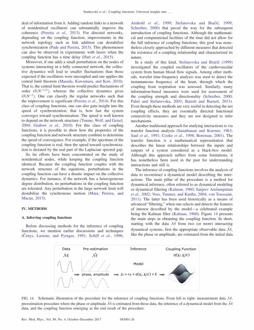
deal of information from it. Adding random links to a networkof nonidentical oscillators can substantially improve thecoherence (Pereira et al., 2013). For directed networks,depending on the coupling function, improvements in thenetwork topology such as link addition can destabilizesynchronization (Pade and Pereira, 2015). This phenomenoncan also be observed in experiments with lasers when thecoupling function has a time delay (Hart et al., 2015).Moreover, if one adds a small perturbation on the nodes of

systems interacting in a fully connected network, the collec-tive dynamics will lead to smaller fluctuations than thoseexpected if the oscillators were uncoupled and one applies thecentral limit theorem (Masuda, Kawamura, and Kori, 2010).That is, the central limit theorem would predict fluctuations oforder OðN−1=2Þ, whereas the collective dynamics givesOðN−1Þ. One can classify the regular networks such thatthe improvement is significant (Pereira et al., 2014). For thisclass of coupling functions, one can also gain insight into thespeed of synchronization, that is, how fast the systemconverges toward synchronization. The speed is well knownto depend on the network structure (Timme, Wolf, and Geisel,2004; Grabow et al., 2010). For this class of couplingfunctions, it is possible to show how the properties of thecoupling function and network structure combine to determinethe speed of convergence. For example, if the spectrum of thecoupling function is real, then the speed toward synchroniza-tion is dictated by the real part of the Laplacian spectral gap.So far efforts have been concentrated on the study of

nonidentical nodes, while keeping the coupling functionidentical. Because the coupling function couples with thenetwork structure of the equations, perturbations in thecoupling function can have a drastic impact on the collectivedynamics. For instance, if the network has a heterogeneousdegree distribution, no perturbations in the coupling functionare tolerated. Any perturbation in the large network limit willdestabilize the synchronous motion (Maia, Pereira, andMacau, 2015).

IV. METHODS

A. Inferring coupling functions

Before discussing methods for the inference of couplingfunctions, we mention earlier discussions and techniques(Čenys, Lasiene, and Pyragas, 1991; Schiff et al., 1996;

Arnhold et al., 1999; Stefanovska and Bračič, 1999;Schreiber, 2000) that paved the way for the subsequentintroduction of coupling functions. Although the mathemati-cal and computational facilities of the time did not allow forthe full inference of coupling functions, this goal was none-theless closely approached by different measures that detectedthe existence of a coupling relationship and characterized itsnature.In a study of this kind, Stefanovska and Bračič (1999)

investigated the coupled oscillators of the cardiovascularsystem from human blood flow signals. Among other meth-ods, wavelet time-frequency analysis was used to detect theinstantaneous frequency of the heart, through which thecoupling from respiration was assessed. Similarly, manyinformation-based measures were used for assessment ofthe coupling strength and directionality (Schreiber, 2000;Paluš and Stefanovska, 2003; Barrett and Barnett, 2013).Even though these methods are very useful in detecting the netcoupling effects, they are essentially directed functionalconnectivity measures and they are not designed to infermechanisms.Another traditional approach for studying interactions is via

transfer function analysis (Sanathanan and Koerner, 1963;Saul et al., 1991; Cooke et al., 1998; Boreman, 2001). Thetransfer function is a mathematical representation thatdescribes the linear relationships between the inputs andoutputs of a system considered as a black-box model.Although this approach suffers from some limitations, ithas nonetheless been used in the past for understandinginteractions and still is.The inference of coupling functions involves the analysis of

data to reconstruct a dynamical model describing the inter-actions. The main pillar of the procedure is a method fordynamical inference, often referred to as dynamical modelingor dynamical filtering (Kalman, 1960; Sanjeev Arulampalamet al., 2002; Voss, Timmer, and Kurths, 2004; von Toussaint,2011). The latter has been used historically as a means ofadvanced “filtering,” when one selects and detects the featuresof interest described by the model—a celebrated examplebeing the Kalman filter (Kalman, 1960). Figure 14 presentsthe main steps in obtaining the coupling function. In short,starting with the data M from two (or more) interactingdynamical systems, first the appropriate observable data ~M,like the phase or amplitude, are estimated from the initial data

FIG. 14. Schematic illustration of the procedure for the inference of coupling functions. From left to right: measurement data M,preestimation procedure where the phase or amplitude ~M is estimated from those data, the inference of a dynamical model from the ~Mdata, and the coupling function emerging as the end result of the procedure.



M, so that they can be used by a method that infers adynamical model from which one can extract the couplingfunctions.The data M are usually represented by amplitude state

signals measured dynamically, i.e., they describe the timeevolution of the system. Very often the raw measurementsrequire preprocessing and preestimation procedures. If thesystems are of an oscillatory nature, the phase of the periodicsignal is extracted; similarly the amplitude can be extractedfrom the signals. There can be further preprocessing, includ-ing filtering within desired intervals, removal of artifacts,noise suppression, removal of common source disturbances,filtering of power supply frequency, etc. The preprocessedsignals then act as input for the inference methods.The inference process aims to reconstruct a model to

describe the interacting dynamical systems. It is given by aset of ordinary differential equations (ODEs) or if there isdynamical noise by stochastic differential equations (SDEs).The model in Fig. 14 is given in terms of general variable χ,while usually the model uses either the phase or amplitudedomain. The dynamics of the system is modeled with a set ofbase functions, which are usually linearly independent. Forexample, the set of base functions can be a Fourier series ofsine and cosine functions. Base functions can be either linearor nonlinear and are specified by a set of parameters c thatusually act as scaling parameters. When appropriately para-metrized by c, the base functions then combine to give the all-important coupling function.The base functions are a part of the model that is assumed to

be known beforehand, so the main task of the inferencemethod is to determine the parameters c from the data ~M,given the (SDE or ODE) model _χ. The choice of the rightmodel can be rather difficult, especially if the dynamicalsystem does not possess some general characteristics.Nevertheless, a number of methods exist for optimal modelselection (Berger and Pericchi, 1996; Ljung, 1998; Burnhamand Anderson, 2002). Given a model and a set of data, one canuse different methods to perform the inference. These methodsmay differ considerably in their characteristics and perfor-mance, and we present some examples of those that are mostwidely used.

B. Methods for coupling function reconstruction

1. Modeling by least-squares fitting

As mentioned, one of the first works on the reconstructionof coupling functions from data was that developed byRosenblum and Pikovsky (2001). Their inference of theinteraction is based on a least-squares fitting procedureapplied to the phase dynamics of the interacting oscillators.The main goal of the method is the detection of coupling anddirectionality. Nevertheless, part of the results are functionsthat closely resemble the form of coupling functions.The technique provides for experimental detection of the

directionality of weak coupling between two self-sustainedoscillators, from bivariate data. The approach makes use of thewell-known fact that weak coupling predominantly affects thephases of the oscillators, not their amplitudes. The principalidea is to investigate and quantify whether the phase dynamics

of one oscillator is influenced by the phase of the other. Toachieve this, the model of the phase equations [Eq. (5)] isfitted to the phase data. From the inferred model and itsparameters, one can then quantify the coupling in one or theother direction.First, for each point in time of the phase time series, the

increments Δ1;2ðkÞ ¼ ϕ1;2ðtk þ τÞ − ϕ1;2ðtkÞ are computed,where τ is a free parameter. These increments Δ1;2ðkÞare considered as being generated by some unknown two-dimensional map

Δ1;2ðkÞ ¼ F 1;2½ϕ1;2ðkÞ;ϕ2;1ðkÞ&:

The functions F 1;2½ϕ1;2ðkÞ;ϕ2;1ðkÞ& are decomposed intoFourier series, and their dependences Δ1;2ðkÞ on ϕ1 and ϕ2

are modeled with the least-square fitting procedure. As basefunctions for the fitting, the Fourier series

F 1;2 ¼X

m;l

Am;leimϕ1þilϕ2 ;

with jlj ≤ 3 for m ¼ 0, jmj ≤ 3 for l ¼ 0, and jlj ¼ jmj ¼ 1were considered.It is worth pointing out that this notion is close to,

although not exactly identical to, the dynamical inferenceof ODEs: the increments Δ1;2ðkÞ are close to the Euler methodfor first order differentiation which would have beenΔEuler;1;2ðkÞ ¼ ½ϕ1;2ðtkþ1Þ − ϕ1;2ðtkÞ&=h, where h is the sam-pling (differentiation) step. Therefore, the functionsF 1;2½ϕ1;2ðkÞ;ϕ2;1ðkÞ& are similar to the coupling functionsq1;2ðϕ1;ϕ2Þ, i.e., they are close to the form of the genuinecoupling functions with close relative but not absolutecoupling strength. Despite the differences, these were prob-ably the first extracted functions of oscillatory interactions,and they were of great importance for the work that followed.The inference itself was performed by least-squares fitting,

a widely used method for finding the best-fitting curve to agiven set of points (Lawson and Hanson, 1974; Leon, 1980).The main objective of the fitting consists of adjusting theparameters of a model function to best fit a data set. The resultof the fitting process is an estimate of parameters, given themodel and the base functions. To obtain the parameterestimates, the least-squares method minimizes the summedsquare of residuals (also often called offsets). The residual℘ðkÞ for the kth data point is defined as the difference betweenthe observed response valueΔðkÞ and the fitted response value~ΔðkÞ and is identified as the error associated with the data. Thesummed square of residuals is then given as

O ¼X

k

℘2ðkÞ ¼X

k

½ΔðkÞ − ~ΔðkÞ&2:

The main estimation, aiming to minimize O, involves partialdifferentiation with respect to each parameter and setting theresult equal to zero (Lawson and Hanson, 1974; Leon, 1980).Such schemes can use linear, weighted, or nonlinear fitting.More recent methods for coupling function reconstructionwith fitting procedures often involve a kernel density estima-tion (Kralemann et al., 2008). The finally inferred parameters



applied to the model base functions provide explicit defini-tions of the functions F 1;2½ϕ1;2ðkÞ;ϕ2;1ðkÞ&.To demonstrate the method, a simple example of two

coupled phase oscillators subject to white noise wasconsidered:

_ϕ1 ¼ ω1 þ ε1 sinðϕ2 − ϕ1Þ þ ξ1ðtÞ;_ϕ2 ¼ ω2 þ ε2 sinðϕ1 − ϕ2Þ þ ξ2ðtÞ;

where the coupling functions are sines of the phase difference[cf. Kuramoto’s coupling function, Eq. (8)], with frequenciesω1;2 ¼ 1) 0.1, and couplings ε1 ¼ 0.1 and ε2 ¼ 0.02 (i.e.,weaker than ε1). The noise is assumed to be white Gaussiannoise with hξ1;2ðtÞξ1;2ðt0Þi¼ δðt− t0Þ2D1;2, where D1;2 ¼ 0.2.Note that the least-squares fitting only infers the deterministicpart of the ODEs, and the noise here is used to introduceimprecisions only, i.e., there is no inference of SDEs.Figure 15 presents the two functions as reconstructed usingleast-squares fitting. Note from Fig. 15(a) that the form of thereconstructed function F 1 rightly resembles that of thegenuine coupling function sinðϕ2 − ϕ1Þ, i.e., a diagonal formof a wave determined by the phase difference ϕ2 − ϕ1; and(b) the strength, or amplitude of F 2, is much lower due to theweaker coupling strength.

2. Dynamical Bayesian inference

The recently introduced method for the dynamical Bayesianinference of coupling functions (Stankovski et al., 2012) relieson a Bayesian framework (Bayes, 1763; Friston, 2002;Smelyanskiy et al., 2005; von Toussaint, 2011) and is appliedto a stochastic differential model where the deterministic partis allowed to be time varying.The method attempts to reconstruct the coupling functions

by inferring a model consisting of two weakly interactingdynamical systems subject to noise. The model to be inferredis described by the stochastic differential equation

_χi ¼ fðχi; χjjcÞ þffiffiffiffiD

pξi; ð32Þ

where i ≠ j ¼ 1; 2, and fðχi; χjjcÞ are base functions describ-ing the deterministic part of the internal and the interactingdynamics. The parameter vector c provides scaling coeffi-cients for the base functions. The noise is assumed to be white,Gaussian, and parametrized by a noise diffusion matrix D. Atthis point we talk of χi in general, but later we refer separatelyto the phase or amplitude coupling functions depending on thedomain of the application.Given the 2 ×M time series X ¼ fχn ≡ χðtnÞg (tn ¼ nh)

provided, and assuming that the model base functions areknown, the main task for dynamical inference is to infer theunknown model parameters and the noise diffusion matrixP ¼ fc;Dg. The problem eventually reduces to maximizationof the conditional probability of observing the parameters P,given the data X . For this Bayes’ theorem (Bayes, 1763) isapplied, exploiting the prior density ppriorðPÞ of the param-eters and the likelihood function lðX jPÞ of observing Xgiven the choice P, in order to determine the posterior densitypX ðPjXÞ of the unknown parameters P conditioned on theobservations X :

pX ðPjXÞ ¼lðX jPÞppriorðPÞRlðX jPÞppriorðPÞdP

:

The next task is to determine the likelihood functions in orderto infer the final posterior result. From the time series themidpoint approximation χ'n ¼ ðχn þ χnþ1Þ=2 is constructed,followed by the Euler differentiation _χn ¼ ðχnþ1 − χnÞ=h.Use of the stochastic integral for noise that is white andindependent leads to the likelihood function, which is givenby a product over n of the probabilities of observing χnþ1 ateach time (Smelyanskiy et al., 2005). The negative log-likelihood function is then S ¼ − lnlðX jPÞ given as

S ¼ N2ln jDjþ h

2

XN−1

n¼0

$ck

∂fkðχ·;nÞ∂χ

þ ½ _χn − ckfkðχ'·;nÞ&TðD−1Þ½ _χn − ckfkðχ'·;nÞ&%; ð33Þ

with implicit summation over the repeated index k. Thelikelihood function (33) is of quadratic form. Thus ifthe prior is a multivariate normal distribution, so also willbe the posterior. Given such a distribution as a prior forthe parameters c, with mean c, and covariance matrix

FIG. 15. The reconstructed functions of the phase interactions.(a) The function F 1ðϕ1;ϕ2Þ for the influence of the second on thefirst oscillator, and (b) the function F 2ðϕ1;ϕ2Þ for the influenceof the first on the second oscillator. From Rosenblum andPikovsky, 2001.



Σprior ≡ Ξ−1prior, the final stationary point of S is calculated

recursively from

D ¼ hNð _χn − ckfkðχ'·;nÞÞTð _χn − ckfkðχ'·;nÞÞ;

ck ¼ ðΞ−1Þkwuw;

uw ¼ ðΞpriorÞkwcw þ hfkðχ'·;nÞðD−1Þ _χn þ −h2

∂fkðχ·;nÞ∂χ ;

Ξkw ¼ ðΞpriorÞkw þ hfkðχ'·;nÞðD−1Þfwðχ'·;nÞ; ð34Þ

where the summation over n ¼ 1;…; N is assumed and thesummation over repeated indices k and w is again implicit.The initial prior distribution can be set to be the noninforma-tive flat normal distribution Ξprior ¼ 0 and cprior ¼ 0. Thesefour equations (34) are the only ones needed for implementingthe method. They are applied to a single block of data X andthe resultant posterior multivariate probability NX ðcjc;ΞÞexplicitly defines the probability density of each parameter setof the model (32).In dynamical Bayesian inference each new prior distribu-

tion depends on and uses the previously inferred posteriordistribution. In this framework, however, the informationpropagation is amended in order to allow the method tofollow the time variability of the parameters (Stankovski et al.,2012). The new prior covariance matrix becomes Σnþ1

prior ¼Σnpost þ Σn

diff , where Σndiff describes how much some part of the

dynamics can change with time.Given the use of Bayesian inference with informative

priors, the method is not prone to the overfitting of parameters,and it does not require much data within the windows because,in each new block of data, it only updates the parameters(Duggento et al., 2012). For analyses of dynamical oscillators,one can use data windows containing 6 to 10 cycles of theslowest oscillation; care is needed to ensure that the windowsare long enough in cases where there is modulation that isslow relative to the eigenfrequencies (Clemson, Lancaster, andStefanovska, 2016). The confidence of the fit is given by theresultant covariance matrix Σpost.This description is for two interacting oscillators.

Nonetheless, the theory also holds for a larger number ofoscillators and the dynamical Bayesian inference has beengeneralized to infer networks of systems with multivariatecoupling functions (Stankovski et al., 2015).Figure 16 shows an application of dynamical Bayesian

inference to cardiorespiratory interactions from a restinghuman subject whose paced respiration was ramped downwith decreasing frequency. The inference of the dynamicsand the coupling functions were reconstructed from thecardiorespiratory phase dynamics (Stankovski et al., 2012).Figure 16(a) indicates the reconstructed respiration frequency,showing the linearly decreasing trend. The inferred couplingdirectionality, defined as Dirc ¼ ðεr − εhÞ=ðεr þ εhÞ, is alsotime varying, with a predominant direction of influence fromthe respiration to the heart. The reconstructed cardiorespira-tory coupling functions [Figs. 16(c)–16(e)] are described bycomplex functions whose form changes qualitatively overtime—cf. Fig. 16(c) with Figs. 16(d) and 16(e). This impliesthat, in contrast to many systems with time-invariant coupling

functions, the functional relations for the interactions of anopen (biological) system can themselves be time-varyingprocesses. By analyzing consecutive time windows, onecan follow the time evolution of the coupling functions.The time variability of biological systems and the ability of

the method to reconstruct it has implications for the detectionof chronotaxic systems, which are a class of nonautonomousself-sustained oscillators able to generate time-varying com-plex dynamics (Suprunenko, Clemson, and Stefanovska,2013). Such systems have drive-response subsystems whichare inherently connected with appropriate coupling functions.Dynamical Bayesian inference has been applied to reconstructsuch chronotaxic systems for cases where the model wasknown or could be closely approximated (Clemson et al.,2014).

3. Maximum likelihood estimation: Multiple shooting

The reconstruction of coupling functions has beenperformed using techniques for maximum likelihood estima-tion, an approach that was employed for reconstruction of thecoupling functions of electrochemical interactions (Tokudaet al., 2007; Tokuda, Wickramasinghe, and Kiss, 2013). Forthis a multiple-shooting method, as one type of maximumlikelihood estimation, was used.The maximum likelihood estimation (Aldrich, 1997;

Myung, 2003) is a statistical method of seeking that proba-bility distribution which makes the observed data most likely,which means that one needs to find the value of the parametervector that maximizes the likelihood function. The procedureof maximization, intuitively describes the “agreement” of theselected model with the observed data, and for discreterandom variables it maximizes the probability of the observeddata under the resulting distribution. The maximum likelihoodestimation gives a unified approach to estimation, which is

FIG. 16. Application of dynamical Bayesian inference tocardiorespiratory interactions when the (paced) respiration istime varying. (a) The inferred time-varying respiration frequency.(b) The coupling directionality between the heart and respi-ration (denoted as h and r, respectively). (c), (d), and (e) Thecardiorespiratory coupling function evaluated for the three timewindows whose positions are indicated by the gray arrows. FromStankovski et al., 2012.



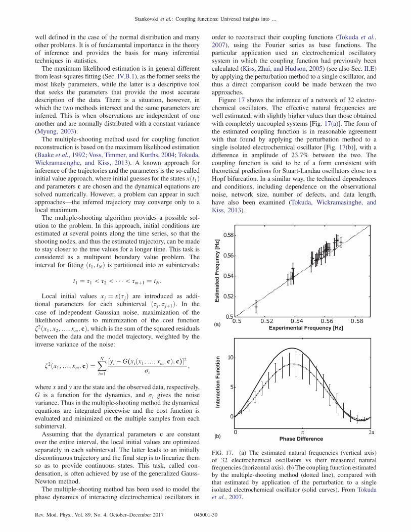
well defined in the case of the normal distribution and manyother problems. It is of fundamental importance in the theoryof inference and provides the basis for many inferentialtechniques in statistics.The maximum likelihood estimation is in general different

from least-squares fitting (Sec. IV.B.1), as the former seeks themost likely parameters, while the latter is a descriptive toolthat seeks the parameters that provide the most accuratedescription of the data. There is a situation, however, inwhich the two methods intersect and the same parameters areinferred. This is when observations are independent of oneanother and are normally distributed with a constant variance(Myung, 2003).The multiple-shooting method used for coupling function

reconstruction is based on the maximum likelihood estimation(Baake et al., 1992; Voss, Timmer, and Kurths, 2004; Tokuda,Wickramasinghe, and Kiss, 2013). A known approach forinference of the trajectories and the parameters is the so-calledinitial value approach, where initial guesses for the states xðt1Þand parameters c are chosen and the dynamical equations aresolved numerically. However, a problem can appear in suchapproaches—the inferred trajectory may converge only to alocal maximum.The multiple-shooting algorithm provides a possible sol-

ution to the problem. In this approach, initial conditions areestimated at several points along the time series, so that theshooting nodes, and thus the estimated trajectory, can be madeto stay closer to the true values for a longer time. This task isconsidered as a multipoint boundary value problem. Theinterval for fitting ðt1; tNÞ is partitioned into m subintervals:

t1 ¼ τ1 < τ2 < ( ( ( < τmþ1 ¼ tN:

Local initial values xj ¼ xðτjÞ are introduced as addi-tional parameters for each subinterval ðτj; τjþ1Þ. In thecase of independent Gaussian noise, maximization of thelikelihood amounts to minimization of the cost functionζ2ðx1; x2;…; xm; cÞ, which is the sum of the squared residualsbetween the data and the model trajectory, weighted by theinverse variance of the noise:

ζ2ðx1;…; xm; cÞ ¼XN

i¼1

½yi −G(xiðx1;…; xm; cÞ; c)&2

σi;

where x and y are the state and the observed data, respectively,G is a function for the dynamics, and σi gives the noisevariance. Thus in the multiple-shooting method the dynamicalequations are integrated piecewise and the cost function isevaluated and minimized on the multiple samples from eachsubinterval.Assuming that the dynamical parameters c are constant

over the entire interval, the local initial values are optimizedseparately in each subinterval. The latter leads to an initiallydiscontinuous trajectory and the final step is to linearize themso as to provide continuous states. This task, called con-densation, is often achieved by use of the generalized Gauss-Newton method.The multiple-shooting method has been used to model the

phase dynamics of interacting electrochemical oscillators in

order to reconstruct their coupling functions (Tokuda et al.,2007), using the Fourier series as base functions. Theparticular application used an electrochemical oscillatorysystem in which the coupling function had previously beencalculated (Kiss, Zhai, and Hudson, 2005) (see also Sec. II.E)by applying the perturbation method to a single oscillator, andthus a direct comparison could be made between the twoapproaches.Figure 17 shows the inference of a network of 32 electro-

chemical oscillators. The effective natural frequencies arewell estimated, with slightly higher values than those obtainedwith completely uncoupled systems [Fig. 17(a)]. The form ofthe estimated coupling function is in reasonable agreementwith that found by applying the perturbation method to asingle isolated electrochemical oscillator [Fig. 17(b)], with adifference in amplitude of 23.7% between the two. Thecoupling function is said to be of a form consistent withtheoretical predictions for Stuart-Landau oscillators close to aHopf bifurcation. In a similar way, the technical dependencesand conditions, including dependence on the observationalnoise, network size, number of defects, and data length,have also been examined (Tokuda, Wickramasinghe, andKiss, 2013).

Est

imat

ed F

requ

ncy

[Hz]

Experimental Frequency [Hz](a)

2

Inte

ract

ion

Func

tion

Phase Difference(b)

FIG. 17. (a) The estimated natural frequencies (vertical axis)of 32 electrochemical oscillators vs their measured naturalfrequencies (horizontal axis). (b) The coupling function estimatedby the multiple-shooting method (dotted line), compared withthat estimated by application of the perturbation to a singleisolated electrochemical oscillator (solid curves). From Tokudaet al., 2007.



4. Random phase resetting method

The method of random phase resetting can be used for thedynamical inference of interacting systems and also for thereconstruction of their coupling functions (Levnajić andPikovsky, 2011). Initially, the method was designed for thereconstruction of network topology, i.e., the inference ofcoupling strengths; nevertheless, the framework employeddynamical inference and the inferred model allows for thecoupling functions to be reconstructed as well.The main idea relies on repeatedly reinitializing the net-

work dynamics (e.g., by performing random phase resets), inorder to produce an ensemble of the initial dynamical data.The quantities obtained by averaging this ensemble reveal thedesired details of the network structure and the couplingfunctions.The method considers a dynamical model of interacting

phase oscillators such as that in Eq. (5), with couplingfunctions in terms of the phase difference qiðϕj − ϕiÞ. Thedynamics starts from a set of initial phases which are denotedas ϕ ¼ ðϕ1;…;ϕNÞðt ¼ 0Þ, chosen from a distributionℏðϕÞ > 0 normalized to ð2πÞN . The method is based ontwo assumptions: (i) that one is able to arbitrarily reinitializethe network dynamics K times, by independently resetting thephases of all nodes to a new state ϕ; and (ii) that one is able tomeasure all the values ϕl, and all initial instantaneousfrequencies _ϕl, each time the dynamics is reinitialized (forl ¼ 1;…;K). A 2π-periodic test function T ¼ T ðϕi − ϕjÞwith zero mean is given as input and the coupling functionsare taken to be represented by a Fourier series, to obtain anexpression for the index ϒij:

ϒij½T & ¼ ð2πÞ−NXN

k¼1

X∞

n¼1

Z

½0;2π&NdϕT ðϕi − ϕjÞ

× ½aðnÞkj sinðnϕk − nϕjÞ þ bðnÞkj cosðnϕk − nϕjÞ&:

The dynamical network described by the phase equationscan be reconstructed by computing ϒij for a suitable Tfunction, e.g., T ðϕÞ ¼ einϕ. The practical implementation interms of the data involves the representation of _ϕl with akernel smoother (Wand and Jones, 1994; Kralemann et al.,2008), and appropriate averaging, to get ϒij½T &:

ϒij½T & ¼& _ϕjT ðϕi − ϕjÞ

ℏðϕÞ

'¼ 1

K

XK

l¼1

_ϕjðϕlÞT ðϕi − ϕjÞℏðϕlÞ

:

To mimic an experimentally feasible situation, K randomphase resets of the network dynamics separated by the timeinterval τ are performed. A network of four phase oscillators,coupled as shown in Fig. 18(a), is considered. After applyingthe inference method, the reconstructed pairwise connectionsare shown to be in reasonable agreement with the actualcoupled values, and especially in identifying the noncou-plings, as shown in Fig. 18(b). Once the parameters of thephase model að1Þij and bð1Þij have been inferred, one can alsoreconstruct the form of the coupling function. Figure 18(c)presents an example of the coupling function showing the

influence that the fourth oscillator is exerting on the secondoscillator.The approach is related to the methods for reconstruction of

phase response curves (see Sec. IV.D.2). Here, however, phaseresetting is used somewhat differently, i.e., the focus is on thenetwork’s internal interactions, rather than on its response tostimuli. The power of this method lies in a framework thatyields both the topology and the coupling functions. Itsdownside is that it is invasive—requiring one to interferewith the ongoing system dynamics (via phase resets orotherwise), which is often experimentally difficult and some-times not even feasible.

5. Stochastic modeling of effective coupling functions

An important feature of the interacting dynamics in realsystems is the presence of noise. Explicit consideration of thestochastic nature of the dynamics can provide a better meansof describing the coupling functions, and how they areaffected. In Sec. IV.B.2 we discussed the dynamicalBayesian method which treats stochastic dynamics, and isable to infer the deterministic part of the coupling functionseparately from the random noise. Often when consideringnoise-induced oscillations, however, one may want to deter-mine the effective coupling functions including the effect ofnoise (Schwabedal and Pikovsky, 2010). When performed on

-1

-0.5

0

0.5

1

12 13 14 21 23 24 31 32 34 41 42 43

a(1) ij

node pairs

-1

-0.5

0

0.5

1

12 13 14 21 23 24 31 32 34 41 42 43

b(1) ij

node pairs

(b)

(a)

(c)

FIG. 18. Inference of interacting dynamics by application of therandom phase resetting method. (a) Four-node network ofinteracting phase oscillators. (b) Reconstruction of the four-nodenetwork. Circles are the actual parameter values and crosses arethe inferred values; left að1Þij , right bð1Þij , for each pair i → j.(c) Coupling function with respect to the phase difference ψ42 ¼ϕ2 − ϕ4 from the reconstructed parameters að1Þ42 and bð1Þ42 . FromLevnajić and Pikovsky, 2011.



the effective phase dynamics with an invariant phase definedin a nonperturbative way, the phase will depend on the noiseintensity, and so will all the corresponding characteristics suchas the coupling function.Schwabedal and Pikovsky considered an effective

phase model describing periodically driven, noise-inducedoscillations

_θ ¼ hðθÞ þ gðθÞξðtÞ þ f(ϑðtÞ; θ); ð35Þ

where ϑ ¼ Ωt is a 2π-periodic driving phase. The aim is todescribe the effective phase dynamics Hðθ; ϑÞ and thecorresponding effective coupling functions. One can expressthe effective dynamics (35) as _θ¼Hðθ;ϑÞ¼HmðθÞþF ðθ;ϑÞ,where HmðθÞ is the ϑ-independent marginal effective velocityand F ðθ; ϑÞ is the effective coupling function. By integratingEq. (35) over ϑ, the marginal effective velocity HmðθÞ can bedetermined. Hence, using F ðθ; ϑÞ ¼ Hðθ; ϑÞ −HmðθÞ, onecan determine the effective coupling function

F ðθ; ϑÞ ¼ f −Z

2π

0f

PPm

dϑ − g2∂θ lnPPm

;

where P ¼ Pðθ; ϑÞ and Pm ¼ PMðθÞ are the probabilitydensities of the full and the marginal dynamics, respectively.The variable θ can be considered as a protophase and can befurther transformed by ϕ ¼ CðθÞ ¼ 2π

Rθ0 PðηÞdη to yield an

invariant effective phase dynamics:

_ϕ ¼ ωþ 2πPm½C−1ðϕÞ&F ½ϑ; C−1ðϕÞ& ¼ ωþ qðϑ;ϕÞ: ð36Þ

Equation (36) provides the effective phase dynamics of theperiodically driven noise-induced oscillations with an effec-tive coupling function q that depends on the noise intensity.This theoretical description can be illustrated on a noise-

driven FitzHugh-Nagumo model as an example of an excit-able system

ϵ _x ¼ x −x3

3− y;

_y ¼ xþ aþ σξðtÞ þ b cosðΩtÞ;

where a ¼ 1.1, ϵ ¼ 0.05 are the parameters of the system, ξðtÞis an additive noise which induces oscillations, and the cosineexternal function provides the interactions in the system. Afterestimation of the protophase time series θ and its trans-formation to the phase ϕ, the effective coupling functionqðΩt;ϕÞ can be determined. For this a double Fourier seriesdecomposition was used with least-squares fitting of themodel to the data. In this sense, the core of the inference isthe same as the least-squares fit discussed in Sec. IV.B.1, eventhough the difference here is that one reconstructs a stochasticmodel.The results of the analysis indicated an increase in the

effective coupling for vanishing noise and masking ofthe coupling for driven noise-induced oscillations of theFitzHugh-Nagumo model. Figure 19 presents an unusualcase with implications for the interpretation of effectivecoupling functions. Namely, the effective coupling function

was computed with two noise intensities for the same couplingstrength. By comparing the two plots in Fig. 19 one can seethat the amplitude of q decreases with increasing noiseintensity. The change in amplitude may have been relatedto a more pronounced masking of the coupling induced by thefrequency shift or due to the generic decrease in effectivecoupling for stronger noise because of flattening of themarginal probability.

6. Comparison and overview of the methods

The methods discussed for reconstruction of couplingfunctions possess some characteristics that are in commonas well other features that differentiate them. The lattereventually lead to different choices of method for use,depending on the circumstances and conditions for thedynamics and the coupling functions to be inferred.Table IV summarizes the difference and performance of the

methods discussed in Sects. IV.B.1–IV.B.5. Inference ofstochastic dynamics, which treated SDEs and the influenceof dynamical noise that can cause noise-induced qualitativechanges (e.g., phase slips), can be performed with dynamicalBayesian inference and stochastic modeling of the effectivecoupling functions. The other methods treat ODEs withpossible measurement noise that can affect the statisticsand precision of the inference.

FIG. 19. Coupling functions for noise-induced oscillations inthe FitzHugh-Nagumo model with b ¼ 0.1 and two differentvalues of the noise intensity D: for (left panel) D ¼ 0.08, themean frequency is ω ≈ 0.62; and for (right panel) D ¼ 0.11,ω ≈ 0.95. From Schwabedal and Pikovsky, 2010.

TABLE IV. Comparison of methods for the inference of couplingfunctions in terms of four characteristics (columns) including,respectively, stochastic treatment, absence of parameter overfitting,calculation speed, and the size of data windows. The methods (rows)are as described in the text: least-square fitting (LSF), dynamicalBayesian inference (DBI), maximum likelihood estimation withmultiple shooting (MLE-MS), random phase resetting (RPR), andthe stochasticmodeling of effective coupling functions (SMECF). The✓ indicates if a method possesses that characteristic, and a × if not.

Stochastic No overfitting Calculation speed Data size

LSF × × ✓ ×DBI ✓ ✓ × ✓MLE-MS × × × ✓RPR × × × ✓SMECF ✓ × ✓ ×



Often the model for inference has more parameters than thereal system. In such cases overfitting of parameters can occurand some methods can infer random error or noise instead ofthe underlying dynamical relationship. A model that has beenoverfitted will generally be a poor representation of the realsystem as it can exaggerate minor fluctuations in the data.Bayesian inference uses informative prior probabilities andcan avoid the problem of overfitting parameters.The speed of calculation varies between methods, especially

as some methods perform additional steps and therefore takelonger. Dynamical Bayesian inference has a recursive loop,evaluated for each timepointwithin a datawindowuntil a certainprecision is reached. The multiple-shooting method requiresadditional initial conditions, the shooting nodes, to be estimatedat several points along the time series. The random phaseresetting method uses a large number of additional randominitial resetting points. These additional processing steps relativeto the initial handling of the time series inevitably require morecomputing power and thus reduce the calculation speed.The coupling functions are usually evaluated for a sequence

of time series each defined by a certain window length whosechoice determines how well a method is able to follow thetime evolution of the coupling functions. Dynamical Bayesianinference updates the new probabilities within a window ofdata, based on prior knowledge; the multiple-shooting methodexploits the initial shooting nodes; and the random-resettingmethod also uses resetting points, which are said to requireshorter data windows and, in turn, to provide good timeresolution of the inference.A difficulty in common for all the methods is the

reconstruction of coupling functions (and coupling strengthin general) when the systems are highly synchronized andcoherent in the 1∶1 frequency ratio (Rosenblum and Pikovsky,2001; Kiss, Zhai, and Hudson, 2005). Namely, in the 1∶1 phasesynchronous state there is a definite strong relationship betweenthe phases and the trajectory on a ðϕ1;ϕ2Þ torus which is oneline; hence ϕ1 and ϕ2 are not independent, and the couplingfunctions of the two variables cannot be separately estimated,i.e., one is not able to separate the effect of interaction from theinternal dynamics of autonomous systems. In order to obtaininformation about the coupling one needs to observe deviationsfrom synchrony, due either to dynamical noise or to the onset ofquasiperiodic dynamics outside the synchronization region.Synchronous states with larger n∶m frequency ratios arefavorable, because many revolutions cover the surface of thetorus, and the inference is then more successful.A similar situation applies for the inference of coupling

functions of dynamical systems in amplitude states. In suchcases, the systems are multidimensional, e.g., two coupledLorenz chaotic systems, and the inference of the couplingfunctions is more plausible in a 1∶1 generalized synchroniza-tion sense (Stankovski, McClintock, and Stefanovska, 2014).Complete synchronization and very strong coupling will againconstrict the available space for inference, leading to diffi-culties in reconstructing the amplitude coupling functions.

C. Toward coupling function analysis

Often one needs to draw conclusions based on comparisonand quantitative measures of the coupling functions, after they

have been inferred. Such situations occur in experimentalstudies of some real system interactions, e.g., in biomedicineor chemistry. For example, the biomedical expert wants tohave a quantitative measure of the coupling functions to beable to describe or compare different states or behaviors inhealth and disease.One needs to quantify some characteristics that describe the

coupling functions, and, in particular, features that are uniqueto the coupling functions and cannot be obtained from othermeasures. The form of the function can describe the mecha-nism of the interactions, so being able to quantify it is ofobvious interest.Quantifying a function is not a trivial task, in general.

However, many coupling functions can be decomposed, or areinferred through decomposition into functional components,such as, for example, when the phase coupling functions aredecomposed into a Fourier series. Therefore, the problem ofquantification of the coupling function can be reduced toquantification of its components, and, in particular, theparameters obtained for the components. In this way, oneis left to work with a one-dimensional vector of parameters.One way to perform such a quantification is through the

correlation coefficient and the difference measure evaluatedfrom the inferred coupling functions (Kralemann et al., 2013).The first index ρ measures the similarity of two couplingfunctions q1 and q2, irrespectively of their coupling strengths.It is calculated as the correlation coefficient

ρ ¼ h ~q1 ~q2ik ~q1kk ~q2k

;

where h∘i denotes spatial averaging over the 2D domain0 ≤ ϕ1, ϕ2 ≤ 2π, ~q ¼ q − hqi, and kqk ¼ hqqi1=2. Thesimilarity index ρ is of great interest as it relates only tothe form of the function and is a unique measure of thecoupling functions. In a similar way, the difference measure isdefined as

η ¼ k ~q1 − ~q2kk ~q1kþ k ~q2k

:

The difference measure is of less interest than ρ as it relates tothe coupling strengths, which can be assessed in differentways through other measures.Two measures were used to analyze the similarity and

difference of cardiorespiratory coupling functions, as shownin Fig. 20. It was found that the functions have a well-pronounced characteristic shape for each of the subjects andthat the correlations between the coupling functions obtainedin different trials with the same subjects were very high[Fig. 20(a)]. Naturally, the correlation between the functionsof different subjects was lower, reflecting the interpersonalvariability; however, it is high enough to demonstrate the highsimilarity of the interactions in the group of subjects. Thesimilarity of the coupling functions, obtained from differentobservables such as the electrocardiograph (ECG) and thearterial pulse for the cardiac oscillations, supports the validityof the use of the invariant phase. The similarity index ρ hasalso been used for quantifying the form of the brain coupling



functions (Stankovski et al., 2015), quantifying significantdifferences in the form of the coupling functions when alteredby the use of different anaesthetics (Stankovski et al., 2016).

D. Connections to other methodological concepts

1. Phase reconstruction procedures

When analyzing data one first needs to reconstruct thephase, before attempting to detect the underlying phasecoupling functions. Various methods exist for phasereconstruction from data, including the marked events method(the marking of a particular time event, e.g., a maximum or azero crossing, within a cycle of oscillation), the Hilberttransform, and wavelet transform based methods (Gabor,1946; Pikovsky, Rosenblum, and Kurths, 2001; Quiroga et al.,2002; Daubechies, Lu, and Wu, 2011; Iatsenko, McClintock,and Stefanovska, 2016). The effect of the method used canhave a direct impact on the form of the reconstructed couplingfunction. It is therefore important to choose a method toreconstruct a phase that is as genuine as possible. For example,the marked events method reduces the intercycle resolutionand, despite its limited usefulness in synchronization analysis,it is not appropriate for coupling function analysis. Kralemannet al. (2008) proposed a protophase-to-phase transform thatobtains an invariant phase in terms of the genuine, observable-independent phases. This technique can be very useful inchecking consistency with the phase estimated by use of theHilbert transform. Some other phase estimates have also beendiscussed, noting that use of the synchrosqueezed wavelettransform means that one does not need explicit protophase-phase preprocessing, as it directly estimates the genuine phase(Daubechies, Lu, and Wu, 2011; Iatsenko et al., 2013).Recently, Schwabedal and Kantz (2016) introduced a methodthat facilitates a phase description of collective, irregular-oscillatory dynamics from multichannel recordings and theydemonstrated it on electroencephalogram (EEG) recordings.Such phase estimates have a potential for the reconstruction ofcoupling functions from collective dynamics. In any case, one

should be careful when estimating phases for couplingfunctions, in particular, from experiments, as otherwise thiscan lead to spurious descriptions of the coupling functions.

2. Relation to phase response curve in experiments

The PRC describes how an oscillator responds to an externalperturbation (Winfree, 1980; Kuramoto, 1984; Tass, 1999).The response of the affected oscillator is manifested as a shiftof its phase. It has been used in various fields, especially inbiological oscillations including the heartbeat, circadianrhythms, and neuronal activity (Czeisler et al., 1989;Ermentrout, 1996; Tass, 1999; Oprisan, Prinz, and Canavier,2004; Preyer and Butera, 2005; Ko and Ermentrout, 2009;Hannay, Booth, and Forger, 2015).The phase response curve is a function expressed in terms

of one phase variable from the affected oscillator (for detailedtheoretical description see Sec. III.B.4). In this way, the phaseresponse curve is a similar concept to a coupling function,with the difference that the latter describes the interactions onthe whole (two-dimensional) space, i.e., depending on the twophase variables. In fact, the phase response curve is a func-tional component of the coupling function. In terms of thegeneral theory of phase dynamics (Winfree, 1980; Kuramoto,1984), the coupling function q1ðϕ1;ϕ2Þ can be expressed asthe product of two functions:

q1ðϕ1;ϕ2Þ ¼ Z1ðϕ1ÞI1ðϕ2Þ; ð37Þ

where Z1ðϕ1Þ is the phase response curve, while I1ðϕ2Þ is theperturbation function.The reconstruction of functional curves from data has been

widely used, elucidating the mechanisms underlying theoscillations found in nature (Czeisler et al., 1989; Tass,1999; Batista et al., 2012). This approach is widely used inneuroscience (Ermentrout, 1996; Galán, Ermentrout, andUrban, 2005; Tateno and Robinson, 2007; Gouwens et al.,2010; Schultheiss, Prinz, and Butera, 2011). For example, thephase response curve has been estimated with electrophysio-logical experiments on real neurons from the mouse olfactorybulb (Galán, Ermentrout, and Urban, 2005). A constantcurrent was injected into the neuron to make it fire at aconstant frequency within the beta or gamma frequency band.By following the responses of the neurons to the injectedcurrent stimulation, the phase response curve was recon-structed. Figure 21(a) shows the experimental dots and thefitted phase response curve, which matches well the one fromthe phase model of the study. The surrogate estimation(shuffled dots) in Fig. 21(b) validates this result. Thus, themethod allowed for a simplification of the complex dynamicsfrom a single neuron to a phase model. This study alsodemonstrates the relationship to the coupling function, whichwas reconstructed from the convolution of the phase responsecurve and the perturbation function—an approach used inchemistry as well (Kiss, Zhai, and Hudson, 2005).Going in the opposite direction, the phase response curve

can be estimated by decomposition of the coupling function(Kralemann et al., 2013). This can be done by decomposingthe reconstructed coupling function into a product of twofunctions [Eq. (37)] and searching for a minimum in the

ES PS EPS EG PG EPG

0

0.2

0.4

0.6

0.8

1

Intrapersonal Interpersonal

ES PS EPS EG PG EPG

0

0.2

0.4

0.6

0.8

1

Intrapersonal Interpersonal(a) (b)

FIG. 20. Box plots illustrating the similarity of cardiorespiratorycoupling functions. (a) The correlation coefficient ρ and (b) thedifference measure η, for all available pairs of functions (highsimilarity corresponds to large ρ and small η). ES: the similaritybetween the respiration-ECG coupling functions of the samesubject, obtained from two trials. EG: the same relation similaritybetween different subjects in the group demonstrates low inter-personal variability. PS and PG: intra- and interpersonal simi-larities, respectively, for the respiration-arterial pulse couplingfunction. EPS and EPG: intra- and interpersonal similarities,respectively, between between the two types of coupling func-tions. From Kralemann et al., 2013.



decomposition error by means of an iterative scheme. In thisway, the interactions coming from the second oscillator areused as the perturbation to the first oscillator under consid-eration, whence there is no need for additional externalstimulation—a procedure referred by Kralemann et al. asan in vivo estimation of the phase response curve. This methodwas applied to the reconstruction of the cardiac phaseresponse curve as perturbed by the respiratory oscillations,as shown in Fig. 22. One can clearly see the interval where thephase response curve is nonzero, so that the cardiac system issusceptible to the respiratory perturbation. Intervals of pos-itive (negative) effective forcing are the intervals whererespiration is accelerating (decelerating) the heart rate.Interesting and relevant parallels could be drawn between

coupling functions and amplitude response curves, or phase-amplitude response curves (Castejón, Guillamon, and Huguet,

2013; Huguet and de la Llave, 2013). The latter are similar tophase response curves, with the difference that there is also aresponse to the amplitude on increasing or decreasing thestrength of the oscillations.

3. General effective connectivity modeling

Quite generally, methods of modeling dynamical systemsfrom data often contain coupling functions (Voss, Timmer,and Kurths, 2004; Smelyanskiy et al., 2005; Friston, 2011;von Toussaint, 2011). The extent to which these couplingfunctions resemble the same concept as that discussed in thisreview can vary, depending on the design of the method andthe model itself. For example, there can be a model of onelarger system which is different from the interaction of two ormany systems, but there can be functions within the modelthat are coupling certain variables or dimensions.Similar implications hold for the general description of

methods for effective connectivity modeling which exploit amodel of differential equations and allow for dynamicalmechanisms of connectivity to be inferred from data. Sucheffective connectivity has particularly wide use in neurosci-ence, where the methods infer the links on different scales ofconnectivity and spatially distributed regions within theheavily connected brain network. Although such methodshave much in common with coupling function inferencemethods they do not, however, consider the coupling functionas an entity, nor do they assess or analyze the couplingfunctions as such.

V. APPLICATIONS AND EXPERIMENTS

In this section we review a number of important applica-tions of the methods for reconstruction of coupling functionsand their use for the study and manipulation of the interactionsin various fields.

A. Chemistry

The interactions of chemical oscillations have beenstudied extensively, including in connection with couplingfunctions (Kiss, Zhai, and Hudson, 2002, 2005; Miyazaki and

0 /2 3 /2 2−0.2

−0.1

0

0.1

0.2

phase angle (rad)

PRC

0 /2 3 /2 2−0.2

−0.1

0

0.1

0.2

phase angle (rad)

PRC

(b)(a)

FIG. 21. Experimental estimation of neuronal phase responsecurves (PRCs). (a) Raw estimation of the PRC (dots) and smooth-ing over a 2π=3 interval (gray line) compared with the estimatedPRC (black line) from the approach in Galán, Ermentrout, andUrban (2005). Both curvesmatch, which indicates that the raw dataare consistent with a phase model. (b) The same as (a) but aftershuffling the raw data. The PRC is roughly flat and yieldsinconsistent results with the smoothing, implying that theshuffled data cannot be described by a phase model. From Galán,Ermentrout, and Urban, 2005.

0

1

2

Z(

e)

e

(a)

susceptible

(a)

RS

T P Q

susceptible

0

1

2

2

I(r)

r

(b)

inspirationexpiration

decelerating

accelerating

FIG. 22. Phase response curve and effective forcing for the cardiorespiratory interactions. (a) Individual PRCs Z and (b) effectiveforcing I for all ECG-based coupling functions (gray curves). In both main panels the thick (blue) lines show the average over all theindividual (gray) curves. The thick (red) lines are obtained by decomposition of the averaged coupling function. The small panel on thetop in (a) shows for comparison the average ECG cycle as a function of its phase. The small panel on the top in (b) shows the averagerespiratory cycle as a function of its phase, with the epochs of inspiration and expiration marked (approximately). From Kralemannet al., 2013.



Kinoshita, 2006; Kiss et al., 2007; Tokuda et al., 2007; Blahaet al., 2011; Tokuda, Wickramasinghe, and Kiss, 2013; Koriet al., 2014). Experiments on chemical, or electrochemical,oscillations provide a convenient way of studying andmanipulating interactions and coupling functions under con-trolled laboratory conditions.One of the more prominent coupling function applications

to chemical oscillators is for engineering complex dynamicalstructures (Kiss et al., 2007). The work exploits the simplicityand analytical tractability of phase models and, in particular,their reconstructed coupling functions in order to designoptimal global, delayed, nonlinear feedback for obtainingand tuning the desired behavior. It uses a feedback designmethodology capable of creating a large class of structuresdescribable by phase models for general self-organizedrhythmic patterns in weakly interacting systems with smallheterogeneities. The electrochemical oscillations wereachieved with electrode potentials during the electrodissolu-tion of nickel wires in sulfuric acid.The engineering of the interactions to the desired behavior is

achieved in a population of N oscillators through the impo-sition of nonlinear, time-delayed feedback in the amplitudestate. This reduces to a phase model of a population ofoscillators with weak, global (all-to-all) coupling describedby the Kuramoto model (Kuramoto, 1984) with a generaldiffusive coupling function qðϕj−ϕiÞ [i.e., notationHðϕj−ϕiÞin this work]. In this way, one can also derive the phaseresponse function ZðϕiÞ in connection to the feedback func-tion. Given such a feedback function and response functionZðϕiÞ, one can in principle obtain the coupling functionqðϕj − ϕiÞ for use in the phase model. However, in the workdiscussed, Kiss et al. (2007) proceeded in the opposite manner:they chose a coupling function to produce the desired statesand then designed a feedback loop with optimized feedbackparameters to give the desired qðϕj − ϕiÞ.The method is demonstrated with three interesting and

important experiments: (i) tuning the desired arbitrary phasedifferences between two dissimilar oscillators (see alsoFig. 1), (ii) generation of complex patterns that includeself-organized switching between unstable dynamical statesand clusters, and (iii) the physiologically important problemof desynchronization of oscillators. Next we devote particularattention to case (ii) involving the generation of sequentialstates and clusters (Ashwin and Timme, 2005).Quadratic feedback to a population of four oscillators is used

to reproduce a coupling function proposed for slow switching;see Fig. 23(a). The experimental system with feedback thatsequentially visits (unstable) two-cluster states with two oscil-lators in each cluster shows two (saddle-type) cluster states instate space; see Fig. 23(b). In agreement with the experiments,the phase model predicted a switch between these states due tothe existence of heteroclinic orbits connecting them. Theseswitches can be seen as a fluctuation of the system order, asshown in Fig. 23(c). The engineered feedback producesconfigurations of two clusters, each containing two elements,connected by heteroclinic orbits. Two types of transitions havebeen observed: intracluster and intercluster transitions aspresented by the trajectories of the experimental system andillustrated as phase space plots in Figs. 23(d) and 23(e).

In a similar way, Kiss, Zhai, and Hudson (2005) developeda method for reconstruction of coupling functions fromelectrochemical oscillations, which are then used to predictsynchronization as also discussed in Sec. II.E. Similarly,Tokuda et al. (2007) and Tokuda, Wickramasinghe, andKiss (2013) used a different technique for inference of thecoupling function of multivariate electrochemical oscillations;see Sec. IV.B.3. Also, to capture the whole nature of theinteraction of electrochemical oscillations (and not only thesynchronization-related ones) the coupling functions werereconstructed in the full two-dimensional (ϕ1;ϕ2) space, i.e.,not only for the one-dimensional diffusive coupling differenceΔϕ ¼ ϕ2 − ϕ1 (Blaha et al., 2011).Of particular interest is a coupling function method that

Miyazaki and Kinoshita (2006) applied for studying theinteractions of Belousov-Zhabotinsky chemical oscillations.This class of reactions serves as a classical example ofnonequilibrium thermodynamics, resulting in the establish-ment of a nonlinear chemical oscillator (Strogatz, 2001). Themethod infers the phase dynamics with diffusive couplingfunctions from the experimental phase time series. The

FIG. 23. Engineering a system of four nonidentical oscillatorsusing a specific coupling function to generate sequentialcluster patterns. (a) The target [solid line, HðΔϕÞ ¼sinðΔϕ1.32Þ0.25 sinð2ΔϕÞ] and optimized coupling functionwith feedback (dashed line). (b) Theoretical and experimentallyobserved heteroclinic orbits and their associated unstablecluster states. (c) Time series of the order parameter [R1 ¼PN

j¼1 expðiϕjÞ] along with some cluster configurations. (d),(e) Trajectories in state space during slow switching. The blacklines represent calculated heteroclinic connections betweencluster states (fixed points). The (red) surface in (e) is the setof trajectories traced out by a heterogeneous phase model.HðΔϕÞon the plots is equivalent to the qðψÞ notation used in the currentreview. From Kiss et al., 2007.



coupling function was already discussed in Sec. II.D, asshown in Fig. 8. Here we further review the interpretation anduse of such coupling functions.The inferred coupling function qðψÞ is used to describe the

mechanisms of the various synchronous states in two mutuallycoupled Belousov-Zhabotinsky reactors. The dynamics of thephase difference ψ can be expressed as

_ψ ¼ −Δω þ εQðψÞ; ð38Þ

whereQðψÞ¼qðψÞ−qð−ψÞ,Δω¼ω2−ω1, and ε ¼ ε12 − ε21.Then, by varying the frequency Δω mismatch and couplingstrength ε, one can study and predict the occurrence ofsynchronization. Figure 24 shows that with the increase ofε, a pair of stationary solutions of Eq. (38) are obtained as theintersection points of QðψÞ and Δω=ε (the first horizontal linefrom the top in Fig. 24). There is one stable solution (solidcircles) and in-phase synchronization is realized. If one furtherincreases ε, a new stable solution appears slightly below π inaddition to that corresponding to in-phase synchronization—the intersection with the second horizontal line from the top inFig. 24. This corresponds to out-of-phase synchronization.Thus, a bistability between out-of-phase and in-phasesynchronization can appear.Kori et al. (2014) performed a comprehensive theoretical

analysis and experimental verification of phenomena inelectrochemical oscillators, investigating the general occur-rence of phase clusters in weakly, globally coupled oscillatorsclose to a Hopf bifurcation. The amplitude equation with ahigher-order correction term, valid near a Hopf bifurcationpoint, is derived and it is used to analytically calculate thephase coupling function from given limit-cycle oscillatormodels. Such phase coupling functions allowed the stabilityof phase clusters to be analyzed as demonstrated on theBrusselator model.Experiments on electrochemical oscillators have demon-

strated the existence of three-cluster states near the Hopfbifurcation with negative coupling. Electric potentials wereused to control the nature of the oscillations, and they were

chosen initially such that the oscillators exhibited smoothoscillations near the Hopf bifurcation. Figure 25(a) showsthe current from one oscillator of each of the three clusters.The nearly balanced three-cluster state with configuration(25∶20∶19) is shown on a grid of 8 × 8 circles in Fig. 25(b).Phase response curves [Fig. 25(c)] and coupling functions[Fig. 25(d)] for these oscillators were found experimentallyby introducing slight perturbations to the oscillations. Thestability of the cluster states was determined, and it was foundthat the three-cluster state is the most stable, while four- andfive-cluster states were observed also at higher potentials.Further increase in the potential resulted in complete desynch-ronization of the 64 oscillators.

B. Cardiorespiratory interactions

The heart and the lungs have physiological functions ofgreat importance for human health and their dysfunction maycorrespond to severe cardiovascular disease. Both organs arecharacterized by a pronounced oscillatory dynamics, and thecardiorespiratory interactions have been studied intensivelyusing the theory and methods from the nonlinear coupled-oscillators approach (Kenner, Passenhofer, and Schwaberger,1976; Schäfer et al., 1998; Stefanovska and Bračič, 1999;Stefanovska et al., 2000).The cardiorespiratory coupling functions are therefore

a subject of great interest, i.e., the mechanisms throughwhich respiration influences the cardiac period and, inparticular, how this relates to different states and diseases.The cardiorespiratory analysis performed with dynamicalBayesian inference (Stankovski et al., 2012), as discussed

FIG. 24. The mechanisms of synchronization for Belousov-Zhabotinsky chemical oscillations as determined by their cou-pling functions. The solid curve shows QðψÞ ¼ qðψÞ − qð−ψÞestimated from the coupling functions qðψÞ. qðψÞ and qð−ψÞ arepresented as dashed and dot-dashed lines, respectively. Stable andunstable solutions of Eq. (38) are shown as solid and open circles,respectively.Δω on the plots is equivalent to theΔω notation usedin this review. From Miyazaki and Kinoshita, 2006.

FIG. 25. Experiments on a three-cluster state close to a Hopfbifurcation with negative global coupling of 64 electrochemicaloscillators. (a) Current time series and the three-cluster configu-ration. Solid, dashed, and dotted curves represent the currentsfrom the three clusters. (b) Cluster configuration. White, black,and gray circles represent the three clusters. (c) Responsefunction and wave form (inset) of the electrode potential froma current of single oscillator. (d) Phase coupling function. ΓðΔϕÞon (d) is equivalent to the qðψÞ notation used in this review. FromKori et al., 2014.



in Sec. IV.B.2 and Fig. 16, revealed the form of the couplingfunctions in detail. The use of a changing respiration fre-quency in a linear (ramped) way showed that the form of thereconstructed coupling functions is in itself time varying.Recently, the method was applied to the study of the effects ofgeneral anesthesia on the cardiorespiratory coupling functions(Stankovski et al., 2016). A similar form of the function wasreconstructed for the awake measurements as in the previousstudies, while its form was more varying and less deterministicfor the state of general anesthesia.Dynamical Bayesian inference was used to study the effect

of ageing on the cardiorespiratory interactions (Iatsenko et al.,2013). Analyses were performed on cardiac and respiratorytime series recorded from 189 subjects of both genders, agedfrom 16 to 90 yr. By application of the synchrosqueezedwavelet transform, the respiratory and cardiac frequencies andphases were preestimated. By applying dynamical Bayesianinference to the phase time series, measures such as synchro-nization, coupling directionality, and the relative contributionsof different mechanisms were then estimated.The cardiorespiratory coupling function was thus recon-

structed, and its time evolution and age dependence wereassessed. Figure 26 shows the time-averaged versions of thecardiorespiratory coupling functions typical of a younger andan older subject. Figures 26(a) and 26(b) show the couplingfunctions of the heart dynamics qhðϕh;ϕrÞ. The form of thefunctions [especially noticeable in Fig. 26(a)] is changingmostly along the respiration phase ϕr axis, while it is nearlyconstant along the ϕh axis, indicating that this coupling ispredominantly defined by the direct influence of respirationon the heart. In physiology, this modulation is known asrespiratory sinus arrythmia (RSA). By comparing the couplingfunctions for the young and old subjects one can see a cleardecrease of the RSA amplitude with age. Note also that RSAremains the main stable contribution to the qhðϕh;ϕrÞcoupling function, irrespective of age and that it survivesafter time averaging. The coupling function from respiratorydynamics qrðϕh;ϕrÞ shown in Figs. 26(c) and 26(d) was verylow and seemed to be quite irregular and not age dependent.From the analysis of the time variability of the form of thecoupling functions it was observed that, in older people, the

heart coupling function qhðϕh;ϕrÞ becomes less stable intime, dominated by the highly time-variable indirect contri-butions. At the same time, the dynamics of the respiratorycoupling function qrðϕh;ϕrÞ did not seem to change with age,being irregular and unstable.Kralemann et al. (2013) looked at the cardiorespiratory

coupling functions, as an intermediate result, in order to obtainthe phase response curve of the heart and the perturbationinserted by respiration. They studied the respiratory andcardiac oscillations of 17 healthy humans while resting inan unperturbed state. The cardiac oscillation was assessedthrough two different observables—the ECG and the arterialpulse signal. The idea of using two different observables is todemonstrate that an invariant phase can be obtained from eachof them, describing a common inherent interaction betweenrespiratory and cardiac oscillations.By analyzing the phase dynamics, first by estimating the

protophases and transforming them into genuine phases, thecardiorespiratory phase coupling functions were recon-structed. Figure 1(b) shows the reconstructed cardiorespira-tory coupling functions Qe using the cardiac phase extractedfrom the ECG signal. The coupling functions estimated fromthe phases of the arterial pulse signal are shown in Fig. 27. Theforms of the functions reveal the detailed mechanism throughwhich respiration influences the cardiac oscillations, i.e., theregions with high values of the function mean higherfrequencies (acceleration), whereas low regions correspondto lower frequencies (deceleration) of the cardiac oscillationsdue to the respiratory influence. The existence of suchcardiorespiratory coupling functions was tested statisticallywith respect to intersubject and intrasubject surrogates.The high similarity of the cardiorespiratory coupling

functions obtained from the phases of the ECG observablesin Fig. 1(b) and those from the arterial pulse phases inFig. 27(b) demonstrates that the proposed method correctlyidentified the underlying interaction mechanism. This wasachieved because the method was able to transform proto-phases from different observables into invariant phase dynam-ics from which a common form of the coupling functions wasobtained. The minor differences in the form of the functions,as compared to the previous one with aging (Fig. 27), are

FIG. 26. Cardiorespiratory coupling functions for the study of human aging. Typical time-averaged coupling functions for (a),(c) a young subject aged 21 yr and (b), (d) an old subject aged 71 yr. (a), (b) are from the cardiac, while (c), (d) are from the respirationphase dynamics. From Iatsenko et al., 2013.



related to possible intersubject variations and the differentphase estimation approaches.The similarity of the cardiorespiratory coupling functions

among different subjects and between the two observablephases was further quantified with the similarity indices(Kralemann et al., 2013), as discussed in Sec. IV.C andshown in Fig. 20. The similarity index that quantifies thecorrelation between the form of the functions also proveduseful in the assessment of the state of general anesthesia(Stankovski et al., 2016). It was found that the intersubjectcorrelation similarity of the cardiorespiratory coupling func-tions, in comparison to the awake state, decreased with theonset of propofol-induced general anesthesia, and to an evengreater extent when sevoflurane was used.

C. Neural coupling functions

Neural states often manifest themselves as changes in brainelectrophysiological activity, which emanates from thedynamics of large-scale cell ensembles oscillating synchro-nously within characteristic frequency intervals. Individualensembles communicate to integrate their local informationflows into a common brain network. One way to describe suchan integration or communication is through cross-frequencycoupling, an approach that has led to numerous studieselucidating the respective roles of cognition, attention,memory, and anesthesia (Canolty et al., 2006; Stefanovska,2007; Lakatos et al., 2008; Jirsa and Müller, 2013). Unlikethese cross-frequency coupling strength approaches, themethods discussed here can assess the neural states throughthe computation of the coupling functions, hence describingthe functional forms and mechanisms of individual cross-frequency interactions. In this way, one infers neural cross-frequency coupling functions (Stankovski et al., 2017).The methods for the reconstruction of coupling functions

have been applied to EEG recordings (Figs. 28 and 29). Thebrain wave intervals, including the δ (0.8–4 Hz), θ (4–7.5 Hz),α (7.5–14 Hz), β (14–22 Hz), and γ (22–80 Hz), were firstextracted from a single EEG channel recording. The phasewas then extracted from each filtered time series, using, forexample, the Hilbert transform or the synchrosqueezed wave-let transform. During this preprocessing procedure, particular

care was taken to minimize overlap between the spectra of theintervals (Lehnertz et al., 2014): overlaps of consecutivefrequency intervals result in overestimation of the correspond-ing phase-to-phase coupling. Dynamical Bayesian inferencewas then used to reconstruct the coupling functions from themultivariate five-phase oscillators. In a similar manner,dynamical Bayesian inference was applied to a study ofneural interactions during epileptic seizures (Wilting andLehnertz, 2015), although not for cross-frequency coupling.As the brain is a highly complex system that can mediate a

variety of functions from fixed structure (Park and Friston,2013), the coupling relationships between the brain waves canbe different. One important coupling relation is the δ; α → α,as it has been found that the δ waves typical of deep sleep inadults can influence the α activity, which is related to theprocessing of information (Feinberg, Floyd, and March, 1987;Jirsa and Müller, 2013). Figure 29(a) shows how the form ofthe δ; α → α coupling functions varies in relation to theirspatial locations on the head. It can be seen that the tridimen-sional waves propagate mostly in the δ dimension. Thistendency can be seen better in Fig. 29(b), which shows theaveraged coupling function. Its form depends predominantlyon the direct delta oscillation, changing mostly along theϕδ axis. This reveals how and when within one cycle the δoscillations accelerate and decelerate the α oscillations. Othercoupling relationships could include, for example, the pair-wise θ; γ → γ and α; γ → γ, or the multivariate tripletθ; α; γ → γ, as shown previously in Fig. 7.Neural cross-frequency coupling functions were used

recently to elucidate the mechanisms of general anesthesia(Stankovski et al., 2016). In fact, the analyses also includedthe cardiac and respiratory oscillations (in a sense integratingSecs. V.B and V.C). Here we review an important findingbased on the neural δ − α coupling functions. The studyincluded 25 awake and 29 anesthetized healthy subjects, ofwhich 14 subjects were anesthetized with the intravenousanaesthetic propofol and 15 subjects with the inhalationalanaesthetic sevoflurane. The aim of the study was to deter-mine if there are any differences in the interaction mechanismswith respect to the three states: awake or anesthetized witheither propofol or sevoflurane.

FIG. 27. Coupling functions for the human cardiorespiratory system. The reconstructed functions specify the dependence of theinstantaneous cardiac frequency, measured in radians per second, on the cardiac and respiratory phases. The functions Qpðϕr;ϕpÞ arecomputed from the arterial pulse and respiration. Results from the subject who had the lowest levels of determinism and similarity to thecoupling functions obtained from ECG phasesQe are shown in (a), and those for the subject with the highest determinism and similarityin (b). (c) The averaged coupling function over all measurements for all subjects. From Kralemann et al., 2013.



Figure 28 shows the group δ − α coupling functions for thethree states. The coupling functions for the awake resting,propofol, and sevoflurane states are evidently quite differentfrom each other, in both the forms and strengths of thecouplings. The δ − α coupling function for the awake state hasa relatively complex and varying form, and low amplitude.The coupling functions for propofol and sevoflurane aresimilar to each other and they look significantly differentfrom those for the awake state. The sevoflurane couplingfunction has the largest coupling amplitude. Careful surrogatetesting showed that the propofol and sevoflurane couplingfunctions are statistically significantly different from thecorresponding surrogates. The qualitative form of the δ − αcoupling function has a sinelike form along the ϕδ axis, whileremaining nearly constant along the ϕα axis. This implies thatmuch of the δ − α coupling comes from the direct contributionof the delta oscillation. The specific form of the function [see,e.g., Fig. 28(c)] reveals the underlying coupling mechanism,i.e., it shows that, when the delta oscillations are between πand 2π, the sine-wave coupling function is higher and the deltaactivity accelerates the alpha oscillations; similarly, when thedelta oscillations are between 0 and π, the coupling function isdecreased and delta decelerates the alpha oscillations.The delta-alpha coupling has been linked to the coding

mechanism of feedback valence information (Cohen et al.,2009), non-REM (rapid eye movement) sleep (Bashan et al.,2012), and the eyes-closed state (Jirsa and Müller, 2013). Thefindings with anesthesia are consistent with, and have furtherextended, these findings. The form of the δ − α couplingfunctions [see, e.g., Fig. 28(c)] indicates that the influence isdirect modulation from delta to alpha, where the couplings aresignificantly stronger in anesthesia than when awake. Thisshowed that, once the subject is anesthetized, delta activityinfluences the alpha oscillations by contributing to thereduction of information processing and integration.

D. Social sciences

In a recent application in social sciences, Ranganathan et al.(2014) and Spaiser et al. (2014) identified the couplingfunctions that capture interactions between social variables,

employing a Bayes factor to decide how many interactionterms should be included in the model.The work presents an interesting study of the relationship

between democracy and economic growth, identifying non-linear relationships between them. Economic growth isassessed through the gross domestic product (GDP) per capita(from the World Bank), while the level of democracy isgauged from the democracy index (from Freedom House)(Ranganathan et al., 2014). It is well known that the GDP percapita and democracy are highly correlated: higher GDPimplies more democracy. The linear Pearson correlationcoefficient between the two variables is 0.571 (p < 0.01).However, by use of coupling functions one can try todetermine a more precise, causal relationship between thevariables, revealing the underlying mechanism.In its general form, the model considered is

_D ¼ q1ðD;GÞ; _G ¼ q2ðD;GÞ;

where D denotes the democracy and G is GDP per capita. Inthis way the change of the variables D and G is representedwith ordinary differential equations, even though the originaldata are discrete and one should really use difference ratherthan differential equations. Nevertheless, this approximationwas used for mathematical simplicity. Further, the model canhave some of the functions from a set of 17 base functions ofpolynomial form, including reciprocal, quadratic, and cubicterms. The main idea of the method is to select the optimalbase functions thereby reducing the number of terms inthe model.The inference itself consists of two main steps. The first is

an inferential fitting to obtain a model from the data, based ona maximum likelihood procedure, and involving multiplelinear regression (similar to that discussed in Sec. IV.B.3). Thesecond step uses a Bayesian (Berger and Pericchi, 1996)model selection procedure.2 Here the method decides howmany interaction terms should be included in the model, i.e., it

FIG. 28. Neural cross-frequency coupling functions between δ and α oscillations in general anesthesia. (a)–(c) The average couplingfunctions from all subjects within the group. Note that, for realistic comparison, the vertical scale of the coupling amplitude is the samein each case. Here “Awake” refers to the state when the subject is conscious and resting, and “Propofol” and “Sevoflurane” to stateswhen the subject is anesthetized with propofol or sevoflurane, respectively. From Stankovski et al., 2016.

2Note that the Bayes factor uses the Bayesian probability theorytoo; however, as it is a purely statistical procedure, it differs from thedynamical Bayesian inference (DBI) as discussed in Sec. IV.B.2.



selects a subgroup of base functions of the 17 polynomialsavailable, after trying all possible combinations among them.Thus, the method punishes overly complicated models andidentifies the models with the most explanatory power. Suchprocedures could greatly benefit if a surrogate testing pro-cedure (see Sec. I.B.2) were used to determine whether thefinally selected model is genuinely reliable.The method was applied to model the interaction of

democracy and GDP per capita for the years 1981–2006for 74 countries. The resulting coupling functions for twoselected models are shown in Fig. 30. The simplestmodel shown in Fig. 30(a) includes a coupling functionwith two terms _D ¼ 0.11G3 − 0.067D=G, while the bestfit five-function model Fig. 30(b) was given as _D ¼0.77G3 þ 1.9D − 0.85D=G − 0.96DG − 0.14D2. For themiddle GDP, both of the coupling functions show depend-ences that closely relate to the linear dependence determinedwith the simple correlation coefficient. However, there weresome nonlinear deviations from this, especially for very lowand very high GDP. In particular, the threshold for very high

GDP indicated that there is no significant improvement indemocracy with further GDP growth.Similarly, the best model for G was inferred to be

_G ¼ 0.014þ 0.0064DG − 0.02G, which shows primarilythat the GDP is growing at a constant rate, but in additiondemonstrates that it is positively affected by democracyinteracting with GDP, and that the growth is self-limiting athigh levels of GDP.Finally, we point out that the method was further applied to

investigate the interactions of other social variables, such asthe case of interactions between democracy, development, andcultural values (Spaiser et al., 2014). These works couldsignificantly benefit from further coupling function assess-ment and analysis.

E. Mechanical coupling functions

Mechanical clocks and oscillators provide an importantcornerstone in the study of interactions and synchronizationphenomena, starting from the earliest observations of thephenomenon in pendulum clocks by Huygens (1673) up to themore comprehensive and detailed studies based on currentmethods (Kapitaniak et al., 2012).Kralemann et al. (2008) described an experiment using two

coupled mechanical metronomes for the analysis of couplingfunctions. The metronomes were placed on a rigid base andthe coupling through which they interact and influence eachother was achieved by connecting them with an elastic rubberband; Fig. 31, top. A digital camera was used for acquiring thedata, from which the oscillatory signals were extracted.Coupling functions were determined for three differentexperimental conditions when (i) the pendulums of themetronomes were linked by a rubber band, (ii) the pendulumswere linked by two rubber bands, and (iii) the metronomeswere uncoupled.From the extracted signals, the Hilbert transform proto-

phases were first estimated and then transformed to genuinephases. The coupling functions were then reconstructed with afitting procedure based on kernel smoothing. Figure 31 shows

FIG. 30. Coupling functions of the change in democracy q1ðD;GÞ, from the interaction between GDP and democracy. (a) The two termmodel, and (b) the five term model. The black lines are the solutions _D ¼ 0. The strengths of the coupling functions are encoded by thecolor bars shown on the side of each figure. From Ranganathan et al., 2014.

FIG. 29. Examples of neural cross-frequency coupling func-tions. (a) Spatial distribution of the δ − α coupling functions overthe head, based on the different probe locations. (b) Averagecoupling function along all the probes for the δ − α couplingrelation. Each δ − α coupling function qαðϕδ;ϕαÞ is evaluatedfrom the α dynamics and depends on the bivariate ðϕδ;ϕαÞphases. From Stankovski et al., 2015.



the results for the three cases. By comparison of the couplingfunctions in the case of one rubber coupling [Figs. 31(a) and31(b)] with the coupling of two rubber couplings [Figs. 31(c)and 31(d)], one can see that the form is very similar, while thecoupling strength is slightly higher for the case of two-bandcoupling. The coupling functions are of a complex form,changing along both axes, thus reflecting the bidirectionalinfluence and contribution within the couplings. The meth-odology correctly detects extremely weak coupling functions[Figs. 31(e) and 31(f)] for the case of no explicit coupling.Future developments of this work could benefit from

comparison of the extracted coupling functions with the actualmechanics of the coupled metronomes, as well as fromvalidation of the weak coupling regime for better justificationof the use of phases.

F. Secure communications

The findings that the cardiorespiratory coupling functioncan be decomposed into a number of independent functions,and that the latter can have a time-varying nature (Stankovskiet al., 2012) (see Sec. V.B), inspired the creation of a new classof secure communications characterized by high efficiencyand modularity (Stankovski, McClintock, and Stefanovska,2014).The protocol (Fig. 32) starts with a number of information

signals coming from different channels or communicationdevices (e.g., mobile phone, sensor networks, or wirelessbroadband) needing to be transmitted simultaneously. Each ofthe signals si is encrypted in an amplitude coupling function;i.e., they serve as scaling parameters in the nonlinear couplingfunctions between two self-sustained systems in the trans-mitter. The coupling functions constitute the private key and,in principle, have an unbounded continuum of possiblecombinations. Two signals, one from each system, are trans-mitted through the public channel. At the receiving end, twosimilar systems are enslaved, i.e., completely synchronized,by the two transmitted signals. Finally, by applying time-evolving dynamical Bayesian inference (as discussed inSec. IV.B.2) to the reconstructed systems, one can infer themodel parameters and decrypt the information signals si.This application is similar to that where amplitude coupling

functions are reconstructed from data. The coupled systemsare multidimensional and may be chaotic Lorenz or Rösslersystems. The great advantage is that the model of the coupledsystems is known exactly on the side of the receiver where theinference is performed. Thus the problem of not knowingthe amplitude model and its dimensionality does not exist. Themain task of the decryption lies in inferring the time evolutionof the parameters.The protocol can encrypt multiple signals simultaneously

as time-evolving parameters. Each of them scales one ofthe coupling functions, which are nonlinear and mutuallylinearly independent. Thus the method inherently allows for

FIG. 31. Coupling functions for the two coupled mechanicalmetronomes. (Top) Experimental apparatus with the two metro-nomes, placed on a rigid support. (a), (b) The coupling functionsin each direction from the case of coupling with one rubber band,(c), (d) with two rubber bands, and (e), (f) coupling functions forthe “uncoupled”without any rubber bands. The vertical scales arethe same so that one can clearly see the reduction of the couplingfunction in the uncoupled case. From Kralemann et al., 2008.

FIG. 32. Schematic diagram showing the communication protocol based on coupling functions. Messages s1;…; sn are encrypted bymodulation of the coupling functions connecting two dynamical systems at the transmitter. Only two signals are transmitted through thepublic domain. The receiver consists of two systems of the same kind with the same coupling functions (forming the private key) anduses dynamical Bayesian inference to reconstruct s1;…; sn. From Stankovski, McClintock, and Stefanovska, 2014.



multiplexing, i.e., simultaneous transmission of multiplesignals. Another property of the protocol is that it is highlyresistant to channel noise. This is because the dynamicalBayesian inference is performed for stochastic dynamics, sothat the method is able very effectively to separate theunwanted noise from the deterministic dynamics carryingthe messages.The method is demonstrated on two bidirectionally coupled

chaotic Lorenz systems. Ten information signals s1;…; s10 areencrypted with ten coupling functions, as indicated on theordinate axis in Fig. 33. The choice of the particular forms ofthe coupling functions prescribes the private key. After thetransmission, the systems are reconstructed on the receiverside and, by application of Bayesian inference, the informa-tion signals are reconstructed. Figure 33 shows good agree-ment of the original with the decrypted bits.

VI. OUTLOOK AND CONCLUSION

A. Future directions and open questions

Coupling functions have been studied as early as some ofthe first theoretical works on interactions and they remain avery active field of research that is attracting increasinginterest from the scientific community. They bring a certaincomplexity in understanding, but at the same time they alsoilluminate, and provide deeper insight into, the interaction

mechanisms. As such, coupling functions pose many openquestions and there still remain many related aspects that arenot well understood. Next we discuss some of the openquestions and current possibilities for further developmentsrelated to coupling functions.

1. Theory

The theoretical development of coupling functions will leadto a better understanding of the mechanisms responsible forthe resulting overall dynamics, and they may help to incor-porate seemingly different models into a general overallframework. Future theoretical studies need to identify theclasses of coupling functions that lead to particular physicaleffects. In doing so, one needs to determine if there are someclasses of functions which demonstrate unique characteristics,and more importantly whether some particular functions leadto common effects. As a consequence, these can then lead toclasses of functions to be used in engineering, for controllingor predicting the outcome of the interactions.The experimental results suggest two important directions

for the theoretical development. First, coupling functions canbe nonautonomous. Secondly, coupling functions can lead tothe coexistence of attractors.The theory of nonautonomous dynamical systems has

gained recent interest, mainly in relation to finite-timebifurcations (Kloeden and Rasmussen, 2011). These math-ematical developments play a major role in the theory ofcoupling functions. The theoretical studies should includesystematic and comprehensive descriptions of the differentclasses of coupling function, including the nonautonomouscase.The coexistence of attractors has gained considerable

attention. As experimental results show, coupling functionsare important especially in relation to network structure andthe effect on the basin of attraction, e.g., the basin of attractionof synchronization. Recent results have shown that the roles ofcoupling function and network structure can be nontrivial(Menck et al., 2013). We still need new theoretical methods totackle problems associated with the involvement of couplingfunctions in the coexistence of attractors. These questions areintimately related to the stability of the system and will play arole in important practical applications, such as to electricalpower grids.

2. Methods

The future development of coupling function methodsneeds to take into account all the advantages and pitfalls ofcurrent methods, e.g., as outlined in the critical comparison inSec. IV.B.6. So far, all the coupling function methods havebeen applied to pairs of coupled systems, or small to mediumsize networks. New methods should allow applications to themore prevalent large-scale networks. In line with this, theyshould aim to achieve faster calculations so as to facilitate theever-growing demand for extensive computation.There is also room for improvements of the amplitude

coupling function methods. The search for more generallyapplicable amplitude models remains open. These should beas general as possible or at least general enough for specificsubsystems.

FIG. 33. Transmission of ten pseudorandom binary signalsencrypted in different coupling functions. The high values (binary“1”) at the transmitter are indicated by gray shading. The receivedsignals, after decrypting, are shown by thick (red) lines, each ofwhich (a)–(j) represents one information signal siðtÞ. Theparticular amplitude coupling functions that were used forencrypting each signal are indicated on the ordinate axis. Thebit words are indicated bym1 −m4 on the top of the figure. FromStankovski, McClintock, and Stefanovska, 2014.



There is a need to overcome the problem of inferringcoupling functions from systems that are highly synchronizedand coherent in 1∶1 frequency ratio. Currently, this is acommon deficiency in all of the available methods forcoupling (function) reconstruction. A possible directionfor solving this issue could lie in the use of perturbation,for example, starting from different initial conditions or withsome other form of temporary deviation from the highlycoherent state.To enhance the inference of more general interactions,

efforts are needed to develop and design robust methods fordistinguishing direct from indirect couplings, better surrogates,and null models for determining significant couplings andinterpretation of the couplings in high-dimensional networks.

3. Analysis

We also point to the need for further development incoupling function analysis: although the basic couplingfunction theory and methods are relatively well developed,there is a pressing need for measures able to exploit thecomputed coupling functions to better effect. The currenttools, including similarity analysis and coupling functiondecomposition, are very useful, but there is a clear need fordevelopment of even more analysis tools. The task here is tofind better and more systematic ways of quantifying anddescribing the form of the coupling functions and the otherfunctional characteristics unique to coupling functions.The development of such methods for analyzing and

characterizing coupling functions could be linked to themathematical theory of functional analysis. To date, thistheory including the main concepts in vector spaces, andmeasures of mappings between the functions, has not yet beenfully exploited in relation to coupling functions.

4. Integration theory applications

We emphasize that further interplay between theory andapplications for the development of coupling functions is stillneeded. Although the applications usually take into accounttheoretical developments, recent experimental findings havenot yet been properly addressed by the theory. For example,the theoretically most studied form of coupling functions isthat for diffusive coupling, which includes the state or phasedifference as an argument. The latter is mostly used because itprovides convenient solvable solutions (see, e.g., the history,Sec. II.B). On the other hand, the coupling decompositionexperiments have shown that it is the direct coupling functionthat often predominates in reality, especially in biologicaloscillatory interactions. Hence, further theoretical studies areneeded to establish the phenomena and the nature of inter-actions for direct coupling functions. Such theoretical inves-tigations can usefully be performed numerically in caseswhere the relevant model cannot be solved analytically.

5. Applications

Coupling functions have universal implications for allinteractions between (dynamical) systems. As such, theycan describe mechanisms operating between systems thatare seemingly of very different natures. We have reviewed a

number of important applications, including, for example,chemical, biomedical, mechanical, social, and secure commu-nications; however, the unique features of coupling functionspromise even further application in these and in other fields.We outline some foreseeable directions for new applications,notwithstanding that many others are also possible.Recently, there has been significant interest and develop-

ments in the study of interactions and synchronization inpower grids (Rohden et al., 2012; Rubido, 2015). To ensure areliable distribution of power, the network should be highlycontrollable and synchronized. It is therefore important thatthe state of synchronization should be highly stable (i.e., deepin the Arnold tongue), so as to ensure that small disruptionsand glitches will not interrupt the function of the network.Coupling functions should be investigated in order to establishhow to design and engineer a persistent (Pereira et al., 2014)and very stable state of synchronization.Similar problems occur with the control, synchronization,

and optimization in transport grids (Rodrigue, 1999;Albrecht, 2004), for example, in a rail network. In such cases,of vital importance are the dynamical and the time-varyingevents. The developed methods and theory for time-varyingcoupling functions could be of great use in these applications.Increasing the scale of the networks often leads to higher-

level organization, including networks of networks and multi-layer networks (Stern, 2013; Kivelä et al., 2014). In such high-dimensional spaces, a variety of different physical effects canbe observed, e.g., synchronization, chimeras, and clustering.The coupling functions of different levels and layers couldprovide deeper insight into the functions or subfunctionintegration of the networks.Coupling functions have been found very useful in studying

the interactions between macroscopic physiological systems,such as those between the cardiorespiratory and neural systemspreviously reviewed. Further coupling function investigationswill probably be developed between different oscillations inintegrated network physiology (Stefanovska, 2007; Bashanet al., 2012). In a similar way, coupling functions betweenmicroscopic physiological organizations could be developed.The latter could explore coupling functions between cellsincluding, for example, the oscillations of neurons or stem cells(Murthy and Fetz, 1996; Jackson et al., 2001; Eytan andMarom, 2006; Méndez-Ferrer et al., 2008).

B. Conclusion

In recent years, the investigation of coupling functions hasdeveloped into a very active and rapidly evolving field. Theirstudy and use have brought much progress in the under-standing of the mechanisms underlying the diverse inter-actions seen in nature. The enterprise has now reached acritical mass, offering increased potential for new and impor-tant discoveries, and in this way the topic has attained asubstance and unity justifying the present review.The concept of the function in the coupling functions is

perhaps its most important characteristic. Yet, preciselybecause of being a function, it is inevitably harder to interpret,assess, and compare than is the case for quantitative measuressuch as the coupling strength. In attempting to integrate andpull together existing knowledge about coupling functions,



therefore, we have tried to organize, to explain, and, as far aspossible, to standardize their description in the hope ofmaking them more generally accessible and useful.Interactions underlie many important phenomena and

functions of the systems found in nature, and it is of greatimportance to be able to describe and understand the mech-anisms through which the interactions occur. Coupling func-tions are opening up new perspectives on these interactionsand we envisage that they will catalyze increased researchactivity on coupled dynamical systems and their interactionsin the future.

ACKNOWLEDGMENTS

We gratefully acknowledge valuable and continuingdiscussions with Ralph Andrzejak, Peter Ashwin, MuriloBaptista, Miroslav Barabash, Chris Bick, Philip Clemson,Andreas Daffertshofer, Andrea Duggento, Jaap Eldering,Deniz Eroglu, Dmytro Iatsenko, Viktor Jirsa, Peter Kloeden,LjupcoKocarev, Thomas Kreuz, Juergen Kurths, Jeroen Lamb,Gemma Lancaster, Klaus Lehnertz, Zoran Levnajić, DmitryLuchinsky, Hiroya Nakao, Milan Paluš, Thomas Peron,Spase Petkoski, Arkady Pikovsky, Antonio Politi, AlbertoPorta, Martin Rasmussen, Francisco Rodrigues, MichaelRosenblum, Rajarshi Roy, Björn Schelter, Ivana Stankovska,Sinisa Stojanovski, Yevhen Suprunenko, Peter Tass, ValentinaTiccinelli, and Dmitry Turaev. The work was supported by theEngineering and Physical Sciences Research Council UK(Grants No. EP/100999X1, No. EP/M015831/1, and No. EP/M006298/1), by the Innovative Training Network COSMOSprogram (funded by the EU Horizon 2020 research andinnovation program under the Marie Sklodowska-CurieGrant Agreement No. 642563), by the Action MedicalResearch UK (Grant No. GN1963), by the LancasterUniversity Department of Physics, by the Fundaçao deAmparo à Pesquisa do Estado de Sao PauloBrazil (Grant No. FAPESP 2013/07375-0), by the Instituteof Pathophysiology and Nuclear Medicine, Faculty ofMedicine, UKIM Skopje, Macedonia, and by the SlovenianResearch Agency (Program No. P20232).

REFERENCES

Abarbanel, H. D. I., R. Brown, J. J. Sidorowich, and L. S. Tsimring,1993, Rev. Mod. Phys. 65, 1331.

Abrams, D. M., and S. H. Strogatz, 2004, Phys. Rev. Lett. 93,174102.

Acebrón, J. A., L. L. Bonilla, C. J. Pérez Vicente, F. Ritort, and R.Spigler, 2005, Rev. Mod. Phys. 77, 137.

Acker, C. D., N. Kopell, and J. A. White, 2003, J. Comput. Neurosci.15, 71.

Aguiar, M., P. Ashwin, A. Dias, and M. Field, 2011, J. Nonlinear Sci.21, 271.

Aguirre, J., R. L. Viana, andM. A. F. Sanjuán, 2009, Rev. Mod. Phys.81, 333.

Albert, R., and A.-L. Barabási, 2002, Rev. Mod. Phys. 74, 47.Albrecht, T., 2004, Computers in Railway Six, edited by J. Allan, C.A. Brebbia, R. J. Hill, G. Sciutto, and S. Sone, Advances inTransport Vol. 15, pp. 885–894.

Aldrich, J., 1997, Stat. Sci. 12, 162.

Andrzejak, R. G., A. Kraskov, H. Stogbauer, F. Mormann, and T.Kreuz, 2003, Phys. Rev. E 68, 066202.

Appleton, E. V., 1923, Proc. Cambridge Philos. Soc. 21, 231[http://ia800202.us.archive.org/23/items/proceedingscambr21camb/proceedingscambr21camb.pdf].

Arenas, A., A. Díaz-Guilera, J. Kurths, Y. Moreno, and C. Zhou,2008, Phys. Rep. 469, 93.

Ariaratnam, J. T., and S. H. Strogatz, 2001, Phys. Rev. Lett. 86, 4278.Arnhold, J., P. Grassberger, K. Lehnertz, and C. E. Elger, 1999,Physica D (Amsterdam) 134, 419.

Aronson, D. G., G. B. Ermentrout, and N. Kopell, 1990, Physica D(Amsterdam) 41, 403.

Ashwin, P., J. Buescu, and I. Stewart, 1994, Phys. Lett. A 193, 126.Ashwin, P., and O. Burylko, 2015, Chaos 25, 013106.Ashwin, P., and M. Timme, 2005, Nonlinearity 18, 2035.Baake, E., M. Baake, H. G. Bock, and K. Briggs, 1992, Phys. Rev. A45, 5524.

Bahraminasab, A., F. Ghasemi, A. Stefanovska, P. V. E. McClintock,and H. Kantz, 2008, Phys. Rev. Lett. 100, 084101.

Balanov, A., N. Janson, D. Postnov, and O. Sosnovtseva, 2008,Synchronization: from Simple to Complex (Springer-Verlag, Berlin).

Baldi, M., 2011, Mon. Not. R. Astron. Soc. 411, 1077.Baptista, M. S., F. M. M. Kakmeni, and C. Grebogi, 2010, Phys. Rev.E 82, 036203.

Barahona, M., and L. M. Pecora, 2002, Phys. Rev. Lett. 89, 054101.Bar-Eli, K., 1985, Physica D (Amsterdam) 14, 242.Barreira, L., and Y. B. Pesin, 2002, Lyapunov Exponents andSmooth Ergodic Theory, Vol. 23 (American Mathematical Society,Providence).

Barrett, A. B., and L. Barnett, 2013, Front. Neuroinf. 7, UNSP 6[https://doi.org/10.3389/fninf.2013.00006].

Baselli, G., A. Porta, O. Rimoldi, M. Pagani, and S. Cerutti, 1997,IEEE Trans. Biomed. Eng. 44, 1092.

Bashan, A., R. P. Bartsch, J. W. Kantelhardt, S. Havlin, and P. C.Ivanov, 2012, Nat. Commun. 3, 702.

Batista, C. A. S., E. L. Lameu, A. M. Batista, S. R. Lopes, T. Pereira,G. Zamora-Lopez, J. Kurths, and R. L. Viana, 2012, Phys. Rev. E86, 016211.

Bayes, T., 1763, Phil. Trans. R. Soc. London 53, 370.Belykh, V. N., I. V. Belykh, and M. Hasler, 2004, Physica D(Amsterdam) 195, 159.

Berger, J. O., and L. R. Pericchi, 1996, J. Am. Stat. Assoc. 91,109.

Bick, C., P. Ashwin, and A. Rodrigues, 2016, Chaos 26, 094814.Bick, C., M. Timme, D. Paulikat, D. Rathlev, and P. Ashwin, 2011,Phys. Rev. Lett. 107, 244101.

Blaha, K. A., A. Pikovsky, M. Rosenblum, M. T. Clark, C. G. Rusin,and J. L. Hudson, 2011, Phys. Rev. E 84, 046201.

Blasius, B., A. Huppert, and L. Stone, 1999, Nature (London) 399,354.

Blasius, B., E. Montbrio, and J. Kurths, 2003, Phys. Rev. E 67,035204.

Blekhman, I. I., 1953, Inzh. Sb. 16, 49 (in Russian).Boccaletti, S., J. Kurths, G. Osipov, D. L. Valladares, and C. S. Zhou,2002, Phys. Rep. 366, 1.

Boccaletti, S., V. Latora, Y. Moreno, M. Chavez, and D.-U. Hwang,2006, Phys. Rep. 424, 175.

Bonilla, L. L., and H. T. Grahn, 2005, Rep. Prog. Phys. 68, 577.Boreman, G. D., 2001,Modulation Transfer Function in Optical andElectro-Optical Systems (SPIE, Bellingham, WA).

Breakspear, M., S. Heitmann, and A. Daffertshofer, 2010, Front.Human Neurosci. 4, 190 [https://doi.org/10.3389/fnhum.2010.00190].




https://doi.org/10.1103/PhysRevLett.93.174102



https://doi.org/10.1023/A:1024474819512

https://doi.org/10.1023/A:1024474819512

https://doi.org/10.1007/s00332-010-9083-9

https://doi.org/10.1007/s00332-010-9083-9




https://doi.org/10.1214/ss/1030037906

https://doi.org/10.1103/PhysRevE.68.066202

http://ia800202.us.archive.org/23/items/proceedingscambr21camb/proceedingscambr21camb.pdf






https://doi.org/10.1016/j.physrep.2008.09.002


https://doi.org/10.1016/S0167-2789(99)00140-2

https://doi.org/10.1016/0167-2789(90)90007-C

https://doi.org/10.1016/0167-2789(90)90007-C

https://doi.org/10.1016/0375-9601(94)90947-4

https://doi.org/10.1063/1.4905197

https://doi.org/10.1088/0951-7715/18/5/009

https://doi.org/10.1103/PhysRevA.45.5524

https://doi.org/10.1103/PhysRevA.45.5524


https://doi.org/10.1111/j.1365-2966.2010.17758.x




https://doi.org/10.1016/0167-2789(85)90182-4

https://doi.org/10.3389/fninf.2013.00006





https://doi.org/10.1109/10.641336

https://doi.org/10.1038/ncomms1705



https://doi.org/10.1098/rstl.1763.0053

https://doi.org/10.1016/j.physd.2004.03.012


https://doi.org/10.1080/01621459.1996.10476668

https://doi.org/10.1080/01621459.1996.10476668

https://doi.org/10.1063/1.4958928



https://doi.org/10.1038/20676

https://doi.org/10.1038/20676



https://doi.org/10.1016/S0370-1573(02)00137-0


https://doi.org/10.1088/0034-4885/68/3/R03

https://doi.org/10.3389/fnhum.2010.00190





Brown, E. N., J. Moehlis, and P. Holmes, 2004, Neural Comput. 16,673.

Brown, R., and L. Kocarev, 2000, Chaos 10, 344.Buck, J., and E. Buck, 1968, Science 159, 1319.Burnham, K. P., and D. R. Anderson, 2002, Model Selection andMultimodel Inference: a Practical Information-Theoretic Approach(Springer, Berlin).

Cabral, J., H. Luckhoo, M. Woolrich, M. Joensson, H. Mohseni, A.Baker, M. L. Kringelbach, and G. Deco, 2014, NeuroImage 90,423.

Canolty, R. T., E. Edwards, S. S. Dalal, M. Soltani, S. S. Nagarajan,H. E. Kirsch, M. S. Berger, N. M. Barbaro, and R. T. Knight, 2006,Science 313, 1626.

Castejón, O., A. Guillamon, and G. Huguet, 2013, J. Math. Neurosci.3, 13.

Čenys, A., G. Lasiene, and K. Pyragas, 1991, Physica D(Amsterdam) 52, 332.

Chicharro, D., and R. G. Andrzejak, 2009, Phys. Rev. E 80, 026217.Christen, M., and W. F. Van Gunsteren, 2008, J. Comput. Chem. 29,157.

Clemson, P., G. Lancaster, and A. Stefanovska, 2016, Proc. IEEE104, 223.

Clemson, P. T., and A. Stefanovska, 2014, Phys. Rep. 542, 297.Clemson, P. T., Y. F. Suprunenko, T. Stankovski, and A. Stefanovska,2014, Phys. Rev. E 89, 032904.

Cohen, M. X., N. Axmacher, D. Lenartz, C. E. Elger, V. Sturm, andT. E. Schlaepfer, 2009, J. Cogn. Neurosci. 21, 875.

Cooke, W. H., J. F. Cox, A. M. Diedrich, J. A. Taylor, L. A. Beightol,J. E. Ames, J. B. Hoag, H. Seidel, and D. L. Eckberg, 1998, Am. J.Physiol. 274, H709 [http://ajpheart.physiology.org/content/274/2/H709.most‑cited].

Cosenza, M. G., and A. Parravano, 2001, Phys. Rev. E 64, 036224.Crawford, J. D., 1995, Phys. Rev. Lett. 74, 4341.Cross, M. C., J. L. Rogers, R. Lifshitz, and A. Zumdieck, 2006, Phys.Rev. E 73, 036205.

Cumin, D., and C. P. Unsworth, 2007, Physica D (Amsterdam) 226,181.

Cuomo, K. M., and A. V. Oppenheim, 1993, Phys. Rev. Lett. 71, 65.Czeisler, C. A., R. E. Kronauer, J. S. Allan, J. F. Duffy, M. E. Jewett,E. N. Brown, and J. M. Ronda, 1989, Science 244, 1328.

Daido, H., 1996a, Phys. Rev. Lett. 77, 1406.Daido, H., 1996b, Physica D (Amsterdam) 91, 24.Daubechies, I., J. Lu, and H. Wu, 2011, Appl. Comput. Harmon.Anal. 30, 243.

DeWoskin, D., W. Geng, A. R. Stinchcombe, and D. B. Forger, 2014,Interface focus 4, 20130076.

Dieci, L., and E. S. Van Vleck, 2002, SIAM J. Numer. Anal. 40, 516.Doidy, J., E. Grace, C. Kühn, F. Simon-Plas, L. Casieri, and D. Wipf,2012, Trends Plant Sci. 17, 413.

Dong, Y., D. Liu, and Z. Yang, 2014, Methods 67, 116.Dorfler, F., and F. Bullo, 2012, SIAM J. Control Optim. 50, 1616.Duggento, A., T. Stankovski, P. V. E. McClintock, and A.Stefanovska, 2012, Phys. Rev. E 86, 061126.

Eldering, J., 2013, Normally Hyperbolic Invariant Manifolds: theNoncompact Case (Springer/Atlantis, Amsterdam).

Engelbrecht, J. R., and R. Mirollo, 2014, Chaos 24, 013114.Ermentrout, B., 1986, in Nonlinear Oscillations in Biologyand Chemistry, edited by H. Othmer (Springer-Verlag, Berlin),pp. 98–114.

Ermentrout, B., 1996, Neural Comput. 8, 979.Ermentrout, B., and D. Saunders, 2006, J. Comput. Neurosci. 20,179.

Ermentrout, G. B., 1981, J. Math. Biol. 12, 327.

Ermentrout, G. B., R. F. Galán, and N. N. Urban, 2008, TrendsNeurosci. 31, 428.

Ermentrout, G. B., and N. Kopell, 1990, SIAM J. Appl. Math. 50,125.

Ermentrout, G. B., and D. H. Terman, 2010, Mathematical Founda-tions of Neuroscience, Vol. 35 (Springer, Dordrecht).

Eroglu, D., J. S. W. Lamb, and T. Pereira, 2017, Contemp. Phys. 58,207.

Eytan, D., and S. Marom, 2006, J. Neurosci. 26, 8465.Faes, L., G. Nollo, and A. Porta, 2011, Phys. Rev. E 83, 051112.Faes, L., A. Porta, and G. Nollo, 2015, Entropy 17, 277.Faraoni, V., M. N. Jensen, and S. A. Theuerkauf, 2006, ClassicalQuantum Gravity 23, 4215.

Farid, B., 1997, Philos. Mag. B 76, 145.Feinberg, I., T. C. Floyd, and J. D. March, 1987, Electroencephalogr.Clin. Neurophysiol. 67, 217.

Feldstein, Y. I., 1992, Space Sci. Rev. 59, 83.Fernandez, B., D. Gérard-Varet, and G. Giacomin, 2014, in AnnalesHenri Poincaré (Springer, New York), pp. 1–31.

Field, M. J., 2015, J. Nonlinear Sci. 25, 779.Filatrella, G., A. H. Nielsen, and N. F. Pedersen, 2008, Eur. Phys. J. B61, 485.

Filatrella, G., N. F. Pedersen, and K. Wiesenfeld, 2000, Phys. Rev. E61, 2513.

Flunkert, V., S. Yanchuk, T. Dahms, and E. Schöll, 2010, Phys. Rev.Lett. 105, 254101.

Frenzel, S., and B. Pompe, 2007, Phys. Rev. Lett. 99, 204101.Friston, K. J., 2002, NeuroImage 16, 513.Friston, K. J., 2011, Brain. Connect. 1, 13.Froyland, G., T. Hüls, G. P. Morriss, and T. M.Watson, 2013, PhysicaD (Amsterdam) 247, 18.

Fujisaka, H., and T. Yamada, 1983, Prog. Theor. Phys. 69, 32.Gaballo, A., F. Zanotti, and S. Papa, 2002, Curr. Protein Peptide Sci.3, 451.

Gabor, D., 1946, J. IEEE 93, 429.Galán, R. F., G. B. Ermentrout, and N. N. Urban, 2005, Phys. Rev.Lett. 94, 158101.

Garcia-Alvarez, D., A. Bahraminasab, A. Stefanovska, and P. V. E.McClintock, 2009, Europhys. Lett. 88, 30005.

Gardiner, C. W., 2004, Handbook of Stochastic Methods (Springer,New York).

Gauthier, D. J., and J. C. Bienfang, 1996, Phys. Rev. Lett. 77, 1751.Ginelli, F., P. Poggi, A. Turchi, H. Chaté, R. Livi, and A. Politi, 2007,Phys. Rev. Lett. 99, 130601.

Glass, L., and M. C. Mackey, 1979, J. Math. Biol. 7, 339.Goldobin, D. S., J. N. Teramae, H. Nakao, and G. B. Ermentrout,2010, Phys. Rev. Lett. 105, 154101.

Golubov, A. A., M. Y. Kupriyanov, and E. IlIchev, 2004, Rev. Mod.Phys. 76, 411.

Gomez-Marin, A., J. Garcia-Ojalvo, and J. M. Sancho, 2007, Phys.Rev. Lett. 98, 168303.

Gouwens, N.W., H. Zeberg, K. Tsumoto, T. Tateno, K. Aihara, andH. P. C. Robinson, 2010, PLoS Comput. Biol. 6, e1000951.

Grabow, C., S. M. Hill, S. Grosskinsky, and M. Timme, 2010,Europhys. Lett. 90, 48002.

Guelfi, A., D. Bestion, M. Boucker, P. Boudier, P. Fillion, M.Grandotto, J.-M. Hérard, E. Hervieu, and P. Péturaud, 2007, Nucl.Sci. Eng. 156, 281.

Hagerstrom, A. M., T. E. Murphy, R. Roy, P. Hövel, I. Omelchenko,and E. Schöll, 2012, Nat. Phys. 8, 658.

Haken, H., 1975, Rev. Mod. Phys. 47, 67.Haken, H., 1983, Synergetics, An Introduction (Springer, Berlin).



https://doi.org/10.1162/089976604322860668

https://doi.org/10.1162/089976604322860668

https://doi.org/10.1063/1.166500

https://doi.org/10.1126/science.159.3821.1319

https://doi.org/10.1016/j.neuroimage.2013.11.047

https://doi.org/10.1016/j.neuroimage.2013.11.047

https://doi.org/10.1126/science.1128115

https://doi.org/10.1186/2190-8567-3-13

https://doi.org/10.1186/2190-8567-3-13

https://doi.org/10.1016/0167-2789(91)90130-2

https://doi.org/10.1016/0167-2789(91)90130-2


https://doi.org/10.1002/jcc.20725

https://doi.org/10.1002/jcc.20725

https://doi.org/10.1109/JPROC.2015.2491262

https://doi.org/10.1109/JPROC.2015.2491262



https://doi.org/10.1162/jocn.2009.21062

http://ajpheart.physiology.org/content/274/2/H709.most-cited














https://doi.org/10.1016/0167-2789(95)00260-X

https://doi.org/10.1016/j.acha.2010.08.002

https://doi.org/10.1016/j.acha.2010.08.002

https://doi.org/10.1098/rsfs.2013.0076

https://doi.org/10.1137/S0036142901392304

https://doi.org/10.1016/j.tplants.2012.03.009

https://doi.org/10.1016/j.ymeth.2013.11.004

https://doi.org/10.1137/110851584


https://doi.org/10.1063/1.4858458

https://doi.org/10.1162/neco.1996.8.5.979

https://doi.org/10.1007/s10827-005-5427-0

https://doi.org/10.1007/s10827-005-5427-0

https://doi.org/10.1007/BF00276920

https://doi.org/10.1016/j.tins.2008.06.002

https://doi.org/10.1016/j.tins.2008.06.002

https://doi.org/10.1137/0150009

https://doi.org/10.1137/0150009

https://doi.org/10.1080/00107514.2017.1345844

https://doi.org/10.1080/00107514.2017.1345844

https://doi.org/10.1523/JNEUROSCI.1627-06.2006


https://doi.org/10.3390/e17010277

https://doi.org/10.1088/0264-9381/23/12/016

https://doi.org/10.1088/0264-9381/23/12/016

https://doi.org/10.1080/01418639708241084

https://doi.org/10.1016/0013-4694(87)90019-8

https://doi.org/10.1016/0013-4694(87)90019-8

https://doi.org/10.1007/BF01262538

https://doi.org/10.1007/s00332-015-9241-1

https://doi.org/10.1140/epjb/e2008-00098-8







https://doi.org/10.1006/nimg.2001.1044

https://doi.org/10.1089/brain.2011.0008



https://doi.org/10.1143/PTP.69.32

https://doi.org/10.2174/1389203023380558

https://doi.org/10.2174/1389203023380558

https://doi.org/10.1049/ji-3-2.1946.0074



https://doi.org/10.1209/0295-5075/88/30005



https://doi.org/10.1007/BF00275153






https://doi.org/10.1371/journal.pcbi.1000951

https://doi.org/10.1209/0295-5075/90/48002

https://doi.org/10.13182/NSE05-98

https://doi.org/10.13182/NSE05-98

https://doi.org/10.1038/nphys2372


Hannay, K. M., V. Booth, and D. B. Forger, 2015, Phys. Rev. E 92,022923.

Hansel, D., G. Mato, and C. Meunier, 1993a, Phys. Rev. E 48,3470.

Hansel, D., G. Mato, and C. Meunier, 1993b, Europhys. Lett. 23,367.

Hart, J. D., J. P. Pade, T. Pereira, T. E. Murphy, and R. Roy, 2015,Phys. Rev. E 92, 022804.

Heagy, J. F., T. L. Carroll, and L. M. Pecora, 1994, Phys. Rev. Lett.73, 3528.

Hens, C. R., O. I. Olusola, P. Pal, and S. K. Dana, 2013, Phys. Rev. E88, 034902.

Higuchi, M., and H. Yasuhara, 2003, Int. J. Mod. Phys. B 17, 3075.Hirsch, M.W., M. Shub, and C. C. Pugh, 1977, Invariant Manifolds(Springer, Berlin).

Hlaváčkováá-Schindler, K., M. Paluš, M. Vejmelka, and J.Bhattacharya, 2007, Phys. Rep. 441, 1.

Hoppensteadt, F. C., and E. M. Izhikevich, 2012, Weakly ConnectedNeural Networks, Vol. 126 (Springer, Dordrecht).

Huang, L., Q. Chen, Y. Lai, and L. M. Pecora, 2009, Phys. Rev. E 80,036204.

Huguet, G., and R. de la Llave, 2013, SIAM J. Appl. Dyn. Syst. 12,1763.

Huygens, C., 1673, The Pendulum Clock or Geometrical Demon-strations Concerning the Motion of Pendula as Applied to Clocks,R. J. Blackwell, trans. 1986 (Iowa State Univ. Press, Ames).

Iatsenko, D., A. Bernjak, T. Stankovski, Y. Shiogai, P. J. Owen-Lynch, P. B. M. Clarkson, P. V. E. McClintock, and A. Stefanovska,2013, Phil. Trans. R. Soc. A 371, 20110622.

Iatsenko, D., P. V. E. McClintock, and A. Stefanovska, 2014, Nat.Commun. 5, 4118.

Iatsenko, D., P. V. E. McClintock, and A. Stefanovska, 2016, SignalProcessing 125, 290.

Ismail, A., and P. Ashwin, 2015, Dyn. Stab. Syst. 30, 122.Izhikevich, E. M., 2000, SIAM J. Appl. Math. 60, 1789.Izhikevich, E. M., 2007, Dynamical Systems in Neuroscience: TheGeometry of Excitability and Bursting (MIT Press, Cambridge,MA).

Jackson, K. A., S. M. Majka, H. Wang, J. Pocius, C. J. Hartley, M.W.Majesky, M. L. Entman, L. H. Michael, K. K. Hirschi, and M. A.Goodell, 2001, J. Clin. Invest. 107, 1395.

Jamšek, J., M. Paluš, and A. Stefanovska, 2010, Phys. Rev. E 81,036207.

Jensen, O., and L. L. Colgin, 2007, Trends Cognit. Sci. 11, 267.Jia, J., Z. Song, W. Liu, J. Kurths, and J. Xiao, 2015, Sci. Rep. 5,17008.

Jirsa, V., and V. Müller, 2013, Frontiers Comput. Neurosci. 7, 78[https://doi.org/10.3389/fncom.2013.00078].

Jones, S., and J. M. Thornton, 1996, Proc. Natl. Acad. Sci. U.S.A. 93,13.

Kalman, R. E., 1960, Trans. ASME—J. Basic Eng. 82, 35.Kapitaniak, M., K. Czolczynski, P. Perlikowski, A. Stefanski, and T.Kapitaniak, 2012, Phys. Rep. 517, 1.

Karnatak, R., R. Ramaswamy, and A. Prasad, 2007, Phys. Rev. E 76,035201.

Karypis, G., and V. Kumar, 2000, VLSI Design 11, 285.Katok, A., and B. Hasselblatt, 1997, Introduction to the ModernTheory of Dynamical Systems, Vol. 54 (Cambridge UniversityPress, Cambridge).

Keller, G., M. Künzle, and T. Nowicki, 1992, Physica D (Amsterdam)59, 39.

Kenner, T., H. Passenhofer, and G. Schwaberger, 1976, PflügersArch. 363, 263.

Keogh, E., and A. Mueen, 2011, in Encyclopedia of MachineLearning, edited by C. Sammut and G. I. Webb (Springer,New York), pp. 257–258.

Khramov, D. M., and C.W. Bielawski, 2007, J. Org. Chem. 72, 9407.Kim, S., S. H. Park, and C. S. Ryu, 1997, Phys. Rev. Lett. 79, 2911.Kiss, I. Z., C. G. Rusin, H. Kori, and J. L. Hudson, 2007, Science316, 1886.

Kiss, I. Z., Y. Zhai, and J. L. Hudson, 2002, Science 296, 1676.Kiss, I. Z., Y. Zhai, and J. L. Hudson, 2005, Phys. Rev. Lett. 94,248301.

Kivelä, M., A. Arenas, M. Barthelemy, J. P. Gleeson, Y. Moreno, andM. A. Porter, 2014, J. Complex Netw. 2, 203.

Kloeden, P. E., and M. Rasmussen, 2011, Nonautonomous Dynami-cal Systems (AMS Mathematical Surveys and Monographs,New York).

Ko, T., and G. B. Ermentrout, 2009, Phys. Rev. E 79, 016211.Kocarev, L., and U. Parlitz, 1995, Phys. Rev. Lett. 74, 5028.Kocarev, L., and U. Parlitz, 1996, Phys. Rev. Lett. 76, 1816.Komarov, M., and A. Pikovsky, 2013, Phys. Rev. Lett. 111, 204101.Kori, H., Y. Kuramoto, S. Jain, I. Z. Kiss, and J. L. Hudson, 2014,Phys. Rev. E 89, 062906.

Koseska, A., E. Volkov, and J. Kurths, 2013a, Phys. Rep. 531, 173.Koseska, A., E. Volkov, and J. Kurths, 2013b, Phys. Rev. Lett. 111,024103.

Kralemann, B., L. Cimponeriu, M. Rosenblum, A. Pikovsky, and R.Mrowka, 2008, Phys. Rev. E 77, 066205.

Kralemann, B., M. Frühwirth, A. Pikovsky, M. Rosenblum, T.Kenner, J. Schaefer, and M. Moser, 2013, Nat. Commun. 4, 2418.

Kralemann, B., A. Pikovsky, and M. Rosenblum, 2011, Chaos 21,025104.

Kralemann, B., A. Pikovsky, and M. Rosenblum, 2013, Phys. Rev. E87, 052904.

Kreuz, T., R. G. Andrzejak, F. Mormann, A. Kraskov, H. Stögbauer,C. E. Elger, K. Lehnertz, and P. Grassberger, 2004, Phys. Rev. E 69,061915.

Kuramoto, Y., 1975, in Lecture Notes in Physics, edited by H. Araki(Springer, New York), Vol. 39, pp. 420–422.

Kuramoto, Y., 1984, Chemical Oscillations, Waves, and Turbulence(Springer-Verlag, Berlin).

Kuramoto, Y., 2015, Video message from Yoshiki Kuramoto to theinternational conference “Dynamics of Coupled Oscillators:40 years of the Kuramoto Model,” held at the Max Planck Institutefor the Physics of Complex Systems, Dresden, Germany, July 27,2015 [https://www.youtube.com/watch?v=lac4TxWyBOg].

Kuramoto, Y., and T. Tsuzuki, 1975, Prog. Theor. Phys. 54, 687.Kurebayashi, W., S. Shirasaka, and H. Nakao, 2013, Phys. Rev. Lett.111, 214101.

Lakatos, P., G. Karmos, A. D. Mehta, I. Ulbert, and C. E. Schroeder,2008, Science 320, 110.

Lancaster, G., Y. F. Suprunenko, K. Jenkins, and A. Stefanovska,2016, Sci. Rep. 6, 29584.

Landa, P. S., 2013, Nonlinear Oscillations and Waves in DynamicalSystems, Vol. 360 (Springer, Dordrecht).

Lawson, C. L., and R. J. Hanson, 1974, Solving Least SquaresProblems, Vol. 161 (SIAM, Philadelphia).

Lehnertz, K., G. Ansmann, S. Bialonski, H. Dickten, C. Geier, and S.Porz, 2014, Physica D (Amsterdam) 267, 7.

Lehnertz, K., and C. E. Elger, 1998, Phys. Rev. Lett. 80, 5019.Le Jan, Y., 1987, Ann. Inst. Henri Poincaré, B 23, 111 [http://www.numdam.org/article/AIHPB_1987__23_1_111_0.pdf].

Leon, S. J., 1980, Linear Algebra with Applications (Macmillan,New York).

Levnajić, Z., and A. Pikovsky, 2011, Phys. Rev. Lett. 107, 034101.







https://doi.org/10.1209/0295-5075/23/5/011

https://doi.org/10.1209/0295-5075/23/5/011






https://doi.org/10.1142/S0217979203020715




https://doi.org/10.1137/120901210

https://doi.org/10.1137/120901210

https://doi.org/10.1098/rsta.2011.0622



https://doi.org/10.1016/j.sigpro.2016.01.024

https://doi.org/10.1016/j.sigpro.2016.01.024

https://doi.org/10.1080/14689367.2014.984917

https://doi.org/10.1137/S0036139999351001

https://doi.org/10.1172/JCI12150



https://doi.org/10.1016/j.tics.2007.05.003

https://doi.org/10.1038/srep17008


https://doi.org/10.3389/fncom.2013.00078





https://doi.org/10.1073/pnas.93.1.13

https://doi.org/10.1073/pnas.93.1.13

https://doi.org/10.1115/1.3662552




https://doi.org/10.1155/2000/19436

https://doi.org/10.1016/0167-2789(92)90205-2

https://doi.org/10.1016/0167-2789(92)90205-2

https://doi.org/10.1007/BF00594612

https://doi.org/10.1007/BF00594612

https://doi.org/10.1021/jo070789x







https://doi.org/10.1093/comnet/cnu016











https://doi.org/10.1063/1.3597647

https://doi.org/10.1063/1.3597647





https://www.youtube.com/watch?v=lac4TxWyBOg










http://www.numdam.org/article/AIHPB_1987__23_1_111_0.pdf





Li, C., and G. Chen, 2004, Physica A (Amsterdam) 343, 263.Liao, L.-D., et al., 2013, Biomedical Engineering 12, 38 [https://doi.org/10.1186/1475‑925X‑12‑38].

Lichtner, M., M. Wolfrum, and S. Yanchuk, 2011, SIAM J. Math.Anal. 43, 788.

Lifton, N. A., J. W. Bieber, J. M. Clem, M. L. Duldig, P. Evenson,J. E. Humble, and R. Pyle, 2005, Earth Planet. Sci. Lett. 239, 140.

Lindner, B., J. Garcia-Ojalvo, A. Neiman, and L. Schimansky-Geier,2004, Phys. Rep. 392, 321.

Ljung, L., 1998, System identification (Springer, Berlin).Lü, J., and G. Chen, 2005, IEEE Trans. Autom. Control 50, 841.Luccioli, S., and A. Politi, 2010, Phys. Rev. Lett. 105, 158104.Ma, Y., and K. Yoshikawa, 2009, Phys. Rev. E 79, 046217.MacKay, R. S., and S. Aubry, 1994, Nonlinearity 7, 1623.Maia, D., T. Pereira, and E. E. Macau, 2015, arXiv:1511.08065.Malkin, I. G., 1956, Some Problems in Nonlinear Oscillation Theory(Gostechizdat, Moscow).

Marklund, M., and P. K. Shukla, 2006, Rev. Mod. Phys. 78, 591.Marvel, S. A., R. E. Mirollo, and S. H. Strogatz, 2009, Chaos 19,043104.

Marvel, S. A., and S. H. Strogatz, 2009, Chaos 19, 013132.Marwan, N., M. C. Romano, M. Thiel, and J. Kurths, 2007, Phys.Rep. 438, 237.

Masuda, N., Y. Kawamura, and H. Kori, 2010, New J. Phys. 12,093007.

Menck, P. J., J. Heitzig, N. Marwan, and J. Kurths, 2013, Nat. Phys.9, 89.

Méndez-Ferrer, S., D. Lucas, M. Battista, and P. S. Frenette, 2008,Nature (London) 452, 442.

Mirollo, R. E., and S. H. Strogatz, 1990, SIAM J. Appl. Math. 50,1645.

Mitchell, G. E., A. Richter, and H. A. Weidenmüller, 2010, Rev.Mod. Phys. 82, 2845.

Miyazaki, J., and S. Kinoshita, 2006, Phys. Rev. Lett. 96, 194101.Mormann, F., K. Lehnertz, P. David, and C. E. Elger, 2000, PhysicaD (Amsterdam) 144, 358.

Murayama, T., 1982, Rev. Geophys. 20, 623.Murthy, V. N., and E. E. Fetz, 1996, J. Neurophysiol. 76, 3968 [http://jn.physiology.org/content/76/6/3968.short].

Myung, I. J., 2003, J. Meth. Psych. 47, 90.Nakao, H., 2015, J. Contemp. Phys. 57, 188.Nakao, H., T. Yanagita, and Y. Kawamura, 2014, Phys. Rev. X 4,021032.

Nawrath, J., M. C. Romano,M. Thiel, I. Z. Kiss, M.Wickramasinghe,J. Timmer, J. Kurths, and B. Schelter, 2010, Phys. Rev. Lett. 104,038701.

Netoff, T. I., M. I. Banks, A. D. Dorval, C. D. Acker, J. S. Haas, N.Kopell, and J. A. White, 2005, J. Neurophysiol. 93, 1197.

Okamoto, K., M. Bosch, and Y. Hayashi, 2009, Physiol. Behav. 24,357.

Omel’chenko,E., andM.Wolfrum, 2012, Phys.Rev. Lett.109, 164101.Oprisan, S. A., A. A. Prinz, and C. C. Canavier, 2004, Biophys. J. 87,2283.

Orosz, G., J. Moehlis, and P. Ashwin, 2009, Prog. Theor. Phys. 122,611.

Ott, E., and T. M. Antonsen, 2008, Chaos 18, 037113.Pade, J. P., and T. Pereira, 2015, Sci. Rep. 5, 9968.Paluš, M., and D. Hoyer, 1998, IEEE Eng. Med. Biol. Mag. 17, 40.Paluš, M., and A. Stefanovska, 2003, Phys. Rev. E 67, 055201(R).Paluš, M., and M. Vejmelka, 2007, Phys. Rev. E 75, 056211.Park, H.-J., and K. Friston, 2013, Science 342, 1238411.Pecora, L. M., and T. L. Carroll, 1990, Phys. Rev. Lett. 64, 821.Pecora, L. M., and T. L. Carroll, 1998, Phys. Rev. Lett. 80, 2109.

Pecora, L. M., F. Sorrentino, A. M. Hagerstrom, T. E. Murphy, and R.Roy, 2014, Nat. Commun. 5, 4079.

Pereira, T., J. Eldering, M. Rasmussen, and A. Veneziani, 2014,Nonlinearity 27, 501.

Pereira, T., D. Eroglu, G. B. Bagci, U. Tirnakli, and H. J. Jensen,2013, Phys. Rev. Lett. 110, 234103.

Petereit, J., and A. Pikovsky, 2017, Commun. Nonlinear Sci. Numer.Simul. 44, 344.

Petkoski, S., and A. Stefanovska, 2012, Phys. Rev. E 86,046212.

Pikovsky, A., and A. Politi, 2016, Lyapunov Exponents: A Toolto Explore Complex Dynamics (Cambridge University Press,Cambridge).

Pikovsky, A., and M. Rosenblum, 2011, Physica D (Amsterdam)240, 872.

Pikovsky, A., M. Rosenblum, and J. Kurths, 2001, Synchronization—A Universal Concept in Nonlinear Sciences (Cambridge UniversityPress, Cambridge).

Pogromsky, A., T. Glad, and H. Nijmeijer, 1999, Int. J. BifurcationChaos Appl. Sci. Eng. 09, 629.

Pogromsky, A., and H. Nijmeijer, 2001, IEEE Trans. Circuits Syst. I48, 152.

Politi, A., and M. Rosenblum, 2015, Phys. Rev. E 91, 042916.Popovych, O. V., Y. L. Maistrenko, and P. A. Tass, 2005, Phys.Rev. E 71, 065201.

Popovych, O. V., S. Yanchuk, and P. A. Tass, 2011, Phys. Rev. Lett.107, 228102.

Prasad, A., 2005, Phys. Rev. E 72, 056204.Prasad, A., M. Dhamala, B. M. Adhikari, and R. Ramaswamy, 2010,Phys. Rev. E 81, 027201.

Preyer, A. J., and R. J. Butera, 2005, Phys. Rev. Lett. 95, 138103.Quiroga, R. Q., A. Kraskov, T. Kreuz, and P. Grassberger, 2002,Phys. Rev. E 65, 041903.

Ranganathan, S., V. Spaiser, R. P. Mann, and D. J. T. Sumpter, 2014,PLoS One 9, e86468.

Rayleigh, J. W. S. B., 1896, The Theory of Sound, Vol. 2 (Macmillan,London).

Resmi, V., G. Ambika, and R. E. Amritkar, 2011, Phys. Rev. E 84,046212.

Rinzel, J., and G. B. Ermentrout, 1998, Methods in NeuronalModeling (MIT Press, Cambridge, MA), pp. 251–291.

Robertson, K. A., and P. Ghazal, 2016, Front. Immunol. 7, 634[https://doi.org/10.3389/fimmu.2016.00634].

Rodrigue, J.-P., 1999, J. Transp. Geog. 7, 255.Rodrigues, F. A., T. K. D. M. Peron, P. Ji, and J. Kurths, 2016, Phys.Rep. 610, 1.

Rohden, M., A. Sorge, M. Timme, and D. Witthaut, 2012, Phys. Rev.Lett. 109, 064101.

Rosenblum, M. G., and A. S. Pikovsky, 2001, Phys. Rev. E 64,045202.

Rosenblum, M. G., A. S. Pikovsky, and J. Kurths, 1996, Phys. Rev.Lett. 76, 1804.

Rubido, N., 2015, Energy Transmission and Synchronizationin Complex Networks: Mathematical Principles (Springer,New York).

Rulkov, N. F., M.M. Sushchik, L. S. Tsimring, and H. D. I.Abarbanel, 1995, Phys. Rev. E 51, 980.

Rul’Kov, N. F., A. R. Volkoskii, A. Rodriguez-Lozano, E. Del Rio,and M. G. Velarde, 1992, Int. J. Bifurcation Chaos 02, 669.

Russo, G., and M. Di Bernardo, 2009, IEEE Trans. Circuits Syst. II56, 177.

Sakaguchi, H., and Y. Kuramoto, 1986, Prog. Theor. Phys. 76,576.



https://doi.org/10.1016/j.physa.2004.05.058

https://doi.org/10.1186/1475-925X-12-38

https://doi.org/10.1186/1475-925X-12-38

https://doi.org/10.1186/1475-925X-12-38

https://doi.org/10.1137/090766796

https://doi.org/10.1137/090766796

https://doi.org/10.1016/j.epsl.2005.07.001


https://doi.org/10.1109/TAC.2005.849233



https://doi.org/10.1088/0951-7715/7/6/006

http://arXiv.org/abs/1511.08065


https://doi.org/10.1063/1.3247089

https://doi.org/10.1063/1.3247089

https://doi.org/10.1063/1.3087132



https://doi.org/10.1088/1367-2630/12/9/093007

https://doi.org/10.1088/1367-2630/12/9/093007



https://doi.org/10.1038/nature06685

https://doi.org/10.1137/0150098

https://doi.org/10.1137/0150098




https://doi.org/10.1016/S0167-2789(00)00087-7

https://doi.org/10.1016/S0167-2789(00)00087-7

https://doi.org/10.1029/RG020i003p00623

http://jn.physiology.org/content/76/6/3968.short





https://doi.org/10.1016/S0022-2496(02)00028-7

https://doi.org/10.1080/00107514.2015.1094987

https://doi.org/10.1103/PhysRevX.4.021032




https://doi.org/10.1152/jn.00982.2004

https://doi.org/10.1152/physiol.00029.2009

https://doi.org/10.1152/physiol.00029.2009


https://doi.org/10.1529/biophysj.104.046193




https://doi.org/10.1063/1.2930766


https://doi.org/10.1109/51.731319







https://doi.org/10.1088/0951-7715/27/3/501


https://doi.org/10.1016/j.cnsns.2016.09.002

https://doi.org/10.1016/j.cnsns.2016.09.002





https://doi.org/10.1142/S0218127499000444

https://doi.org/10.1142/S0218127499000444

https://doi.org/10.1109/81.904879

https://doi.org/10.1109/81.904879










https://doi.org/10.1371/journal.pone.0086468



https://doi.org/10.3389/fimmu.2016.00634





https://doi.org/10.1016/S0966-6923(99)00018-6










https://doi.org/10.1142/S0218127492000781

https://doi.org/10.1109/TCSII.2008.2011611

https://doi.org/10.1109/TCSII.2008.2011611



Sanathanan, C., and J. Koerner, 1963, IEEE Trans. Autom. Control 8,56.

Sanjeev Arulampalam, M., S. Maskell, N. Gordon, and T. Clapp,2002, IEEE Trans. Signal Process. 50, 174.

Saul, J. P., R. D. Berger, P. Albrecht, S. P. Stein., M. H. Chen, andR. J. Cohen, 1991, Am. J. Physiol. 261, H1231 [http://ajpheart.physiology.org/content/261/4/H1231.short].

Saxena, G., A. Prasad, and R. Ramaswamy, 2012, Phys. Rep. 521,205.

Schäfer, C., M. G. Rosenblum, J. Kurths, and H. H. Abel, 1998,Nature (London) 392, 239.

Schiff, S. J., P. So, T. Chang, R. E. Burke, and T. Sauer, 1996, Phys.Rev. E 54, 6708.

Schindler, K., H. Leung, C. E. Elger, and K. Lehnertz, 2007, Brain130, 65.

Schneider, I., M. Kapeller, S. Loos, A. Zakharova, B. Fiedler, and E.Schöll, 2015, Phys. Rev. E 92, 052915.

Schreiber, T., 2000, Phys. Rev. Lett. 85, 461.Schreiber, T., and A. Schmitz, 2000, Physica D (Amsterdam) 142,346.

Schultheiss, N.W., A. A. Prinz, and R. J. Butera, 2011, PhaseResponse Curves in Neuroscience: Theory, Experiment, andAnalysis (Springer Science & Business Media, Berlin).

Schwabedal, J. T., and A. Pikovsky, 2010, Phys. Rev. E 81,046218.

Schwabedal, J. T. C., and H. Kantz, 2016, Phys. Rev. Lett. 116,104101.

Schwabedal, J. T. C., D. E. Knapper, and A. L. Shilnikov, 2016,Nonlinearity 29, 3647.

Shukla, P. K., and B. Eliasson, 2011, Rev. Mod. Phys. 83, 885.Skardal, P. S., E. Ott, and J. G. Restrepo, 2011, Phys. Rev. E 84,036208.

Smale, S., 1976, in The Hopf Bifurcation and its Applications(Springer, New York), pp. 354–367.

Smeal, R. M., G. B. Ermentrout, and J. A. White, 2010, Phil. Trans.R. Soc. B 365, 2407.

Smelyanskiy, V. N., D. G. Luchinsky, A. Stefanovska, and P. V. E.McClintock, 2005, Phys. Rev. Lett. 94, 098101.

Smirnov, D. A., and B. P. Bezruchko, 2009, Phys. Rev. E 79, 046204.Sorrentino, F., M. di Bernardo, F. Garofalo, and G. Chen, 2007, Phys.Rev. E 75, 046103.

Spaiser, V., S. Ranganathan, R. P. Mann, and D. J. T. Sumpter, 2014,PLoS One 9, e97856.

Stam, C. J., A. M. V.-C. van Walsum, Y. A. L. Pijnenburg, H.W.Berendse, J. C. de Munck, P. Scheltens, and B.W. van Dijk, 2002,J. Clin. Neurophysiol. 19, 562.

Stamenović, D., and D. E. Ingber, 2009, Soft Matter 5, 1137.Staniek, M., and K. Lehnertz, 2008, Phys. Rev. Lett. 100, 158101.Stankovski, T., A. Duggento, P. V. E. McClintock, and A.Stefanovska, 2012, Phys. Rev. Lett. 109, 024101.

Stankovski, T., P. V. E. McClintock, and A. Stefanovska, 2014, Phys.Rev. X 4, 011026.

Stankovski, T., S. Petkoski, J. Raeder, A. F. Smith, P. V. E.McClintock, and A. Stefanovska, 2016, Phil. Trans. R. Soc. A374, 20150186.

Stankovski, T., V. Ticcinelli, P. V. E. McClintock, and A.Stefanovska, 2015, New J. Phys. 17, 035002.

Stankovski, T., V. Ticcinelli, P. V. E. McClintock, and A.Stefanovska, 2017, Front. Syst. Neurosci. 11.

Stefanovska, A., 2007, IEEE Eng. Med. Biol. Mag. 26, 25.Stefanovska, A., and M. Bračič, 1999, Contemp. Phys. 40, 31.Stefanovska, A., H. Haken, P. V. E. McClintock, M. Hožič,F. Bajrović, and S. Ribarič, 2000, Phys. Rev. Lett. 85, 4831.

Stepowski, D., 1992, Prog. Energy Combust. Sci. 18, 463.Stern, P., 2013, Science 342, 577.Steur, E., I. Tyukin, and H. Nijmeijer, 2009, Physica D (Amsterdam)238, 2119.

Stiefel, K. M., B. S. Gutkin, and T. J. Sejnowski, 2008, PLoS One 3,e3947.

Strogatz, S., 2001, Nonlinear Dynamics And Chaos (Westview Press,Boulder).

Strogatz, S. H., 2000, Physica D (Amsterdam) 143, 1.Strogatz, S. H., 2003, Sync: The Emerging Science of SpontaneousOrder (Hyperion, New York).

Strogatz, S. H., and R. E. Mirollo, 1991, J. Stat. Phys. 63, 613.Suárez-Vargas, J. J., J. A. González, A. Stefanovska, and P. V. E.McClintock, 2009, Europhys. Lett. 85, 38008.

Sun, J., E. M. Bollt, and T. Nishikawa, 2009, Europhys. Lett. 85,60011.

Sun, J., D. Taylor, and E. M. Bollt, 2015, SIAM J. Appl. Dyn. Syst.14, 73.

Suprunenko, Y. F., P. T. Clemson, and A. Stefanovska, 2013, Phys.Rev. Lett. 111, 024101.

Takens, F., 1981, in Lecture Notes in Mathematics, edited by D. A.Rand and L. S. Young (Springer-Verlag, New York), Vol. 898,pp. 366–381.

Tass, P., M. G. Rosenblum, J. Weule, J. Kurths, A. Pikovsky, J.Volkmann, A. Schnitzler, and H.-J. Freund, 1998, Phys. Rev. Lett.81, 3291.

Tass, P. A., 1999, Phase Resetting in Medicine and Biology (Springer,Berlin).

Tateno, T., and H. P. C. Robinson, 2007, Biophys. J. 92, 683.Teasdale, R. D., and M. R. Jackson, 1996, Annu. Rev. Cell Dev. Biol.12, 27.

Teramae, J. N., H. Nakao, and G. B. Ermentrout, 2009, Phys. Rev.Lett. 102, 194102.

Ticcinelli, V., et al., 2017, Frontiers in Physiology (in press).Timme, M., 2007, Phys. Rev. Lett. 98, 224101.Timme, M., F. Wolf, and T. Geisel, 2004, Phys. Rev. Lett. 92,074101.

Tokuda, I. T., S. Jain, I. Z. Kiss, and J. L. Hudson, 2007, Phys. Rev.Lett. 99, 064101.

Tokuda, I. T., M. Wickramasinghe, and I. Z. Kiss, 2013, Phys. Lett. A377, 1862.

Tompkins, N., N. Li, C. Girabawe, M. Heymann, G. B. Ermentrout,I. R. Epstein, and S. Fraden, 2014, Proc. Natl. Acad. Sci. U.S.A.111, 4397.

Turaev, D., 2015, Commun. Math. Phys. 335, 1235.Turing, A. M., 1952, Phil. Trans. R. Soc. B 237, 37.Ullner, E., and A. Politi, 2016, Phys. Rev. X 6, 011015.Urban, A., and B. Ermentrout, 2012, Phys. Rev. E 86, 011907.Van der Pol, B., 1927, Lond. Edinb. Dublin Phil. Mag. J. Sci. 3, 65.Venkataramani, S. C., B. R. Hunt, E. Ott, D. J. Gauthier, and J. C.Bienfang, 1996, Phys. Rev. Lett. 77, 5361.

Viana, R. L., C. Grebogi, S. E. d. Pinto, S. R. Lopes, A. M. Batista,and J. Kurths, 2005, Physica D (Amsterdam) 206, 94.

Vladimirov, A. G., G. Kozyreff, and P. Mandel, 2003, Europhys. Lett.61, 613.

Vlasov, V., E. E. N. Macau, and A. Pikovsky, 2014, Chaos 24,023120.

Vlasov, V., and A. Pikovsky, 2013, Phys. Rev. E 88, 022908.Vlasov, V., Y. Zou, and T. Pereira, 2015, Phys. Rev. E 92, 012904.von Toussaint, U., 2011, Rev. Mod. Phys. 83, 943.Voss, H. U., J. Timmer, and J. Kurths, 2004, Int. J. Bifurcation Chaos14, 1905.



https://doi.org/10.1109/TAC.1963.1105517

https://doi.org/10.1109/TAC.1963.1105517

https://doi.org/10.1109/78.978374

http://ajpheart.physiology.org/content/261/4/H1231.short






https://doi.org/10.1038/32567



https://doi.org/10.1093/brain/awl304

https://doi.org/10.1093/brain/awl304



https://doi.org/10.1016/S0167-2789(00)00043-9

https://doi.org/10.1016/S0167-2789(00)00043-9





https://doi.org/10.1088/0951-7715/29/12/3647




https://doi.org/10.1098/rstb.2009.0292







https://doi.org/10.1097/00004691-200212000-00010

https://doi.org/10.1039/B806442C







https://doi.org/10.1088/1367-2630/17/3/035002

https://doi.org/10.3389/fnsys.2017.00033

https://doi.org/10.1109/EMB.2007.907088

https://doi.org/10.1080/001075199181693


https://doi.org/10.1016/0360-1285(92)90035-Y

https://doi.org/10.1126/science.342.6158.577





https://doi.org/10.1016/S0167-2789(00)00094-4

https://doi.org/10.1007/BF01029202

https://doi.org/10.1209/0295-5075/85/38008

https://doi.org/10.1209/0295-5075/85/60011

https://doi.org/10.1209/0295-5075/85/60011

https://doi.org/10.1137/140956166

https://doi.org/10.1137/140956166






https://doi.org/10.1146/annurev.cellbio.12.1.27









https://doi.org/10.1016/j.physleta.2013.05.016

https://doi.org/10.1016/j.physleta.2013.05.016

https://doi.org/10.1073/pnas.1322005111

https://doi.org/10.1073/pnas.1322005111

https://doi.org/10.1007/s00220-015-2338-4




https://doi.org/10.1080/14786440108564176



https://doi.org/10.1209/epl/i2003-00115-8

https://doi.org/10.1209/epl/i2003-00115-8

https://doi.org/10.1063/1.4880835

https://doi.org/10.1063/1.4880835




https://doi.org/10.1142/S0218127404010345

https://doi.org/10.1142/S0218127404010345

Wand, M. P., and M. C. Jones, 1994, Kernel Smoothing (CRC Press,Boca Raton, FL).

Ward, J. P. T., 2008, Biochim. Biophys. Acta 1777, 1.Watanabe, S., and S. H. Strogatz, 1993, Phys. Rev. Lett. 70, 2391.Wei, C.-J., X. Xu, and C.W. Lo, 2004, Annu. Rev. Cell Dev. Biol. 20,811.

Weighill, D. A., and D. A. Jacobson, 2015, PLoS Comput. Biol. 11,e1004079.

Wiener, N., 1963, Cybernetics (supplementary chapters) (Eyre andSpottiswoode, London).

Wiesenfeld, K., P. Colet, and S. H. Strogatz, 1996, Phys. Rev. Lett.76, 404.

Wiesenfeld, K., P. Colet, and S. H. Strogatz, 1998, Phys. Rev. E 57,1563.

Wiggins, S., 2013, Normally Hyperbolic Invariant Manifolds inDynamical Systems (Springer, Dordrecht).

Williams, C. R. S., T. E. Murphy, R. Roy, F. Sorrentino, T. Dahms,and E. Schöll, 2013, Phys. Rev. Lett. 110, 064104.

Wilting, J., and K. Lehnertz, 2015, Eur. Phys. J. B 88, 193.Winfree, A. T., 1967, J. Theor. Biol. 16, 15.

Winfree, A. T., 1980, The Geometry of Biological Time (Springer-Verlag, New York).

Wojcik J., J. Schwabedal, R. Clewley, and A. L. Shilnikov, 2014,PLoS One 9, e92918.

Yanchuk, S., Y. Maistrenko, and E. Mosekilde, 2001, Physica D(Amsterdam) 154, 26.

Yeung, M. K. S., and S. H. Strogatz, 1999, Phys. Rev. Lett. 82,648.

Yoshimura, K., and K. Arai, 2008, Phys. Rev. Lett. 101,154101.

Zakharova, A., M. Kapeller, and E. Schöll, 2014, Phys. Rev. Lett.112, 154101.

Zakharova, A., I. Schneider, Y. N. Kyrychko, K. B. Blyuss, A.Koseska, B. Fiedler, and E. Schöll, 2013, Europhys. Lett. 104,50004.

Zass, R., and A. Shashua, 2008, in Proc. IEEE Conf. on ComputerVision and Pattern Recognition (CVPR 2008) (IEEE, New York),pp. 1–8.

Zhai, Y., I. Z. Kiss, and J. L. Hudson, 2004, Phys. Rev. E 69, 026208.Zhang, L., 2013, Superlattices Microstruct. 53, 113.



https://doi.org/10.1016/j.bbabio.2007.10.010












https://doi.org/10.1016/0022-5193(67)90051-3


https://doi.org/10.1016/S0167-2789(01)00221-4

https://doi.org/10.1016/S0167-2789(01)00221-4







https://doi.org/10.1209/0295-5075/104/50004

https://doi.org/10.1209/0295-5075/104/50004


https://doi.org/10.1016/j.spmi.2012.09.016

Coupling functions: Universal insights into dynamical ...

Documents

Transcript of Coupling functions: Universal insights into dynamical ...