Coupling Di erent Tra c Models - UCLAhelper.ipam.ucla.edu/publications/traws1/traws1_13185.pdf ·...
73
Coupling Different Traffic Models Francesca Marcellini Department of Mathematics and Applications University of Milano–Bicocca, Italy September 28th - October 2nd, 2015 Mathematical Foundations of Traffic IPAM, UCLA, Los Angeles, USA
-
Upload
trinhduong -
Category
Documents
-
view
215 -
download
0
Transcript of Coupling Di erent Tra c Models - UCLAhelper.ipam.ucla.edu/publications/traws1/traws1_13185.pdf ·...
Coupling Different Traffic Models
Francesca Marcellini
Department of Mathematics and ApplicationsUniversity of Milano–Bicocca, Italy
September 28th - October 2nd, 2015
Mathematical Foundations of TrafficIPAM, UCLA, Los Angeles, USA

Introduction
A Two-Phase Model
A Discrete–Continuous Description
A Traffic Model Aware of Real Time Data

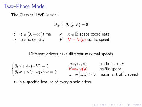
Two–Phase Model
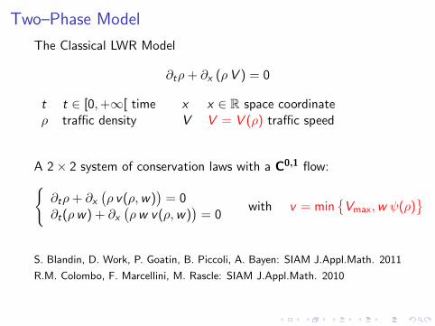
The Classical LWR Model
∂tρ+ ∂x (ρV ) = 0
t t ∈ [0,+∞[ time x x ∈ R space coordinateρ traffic density V V = V (ρ) traffic speed

Two–Phase Model
The Classical LWR Model
∂tρ+ ∂x (ρV ) = 0
t t ∈ [0,+∞[ time x x ∈ R space coordinateρ traffic density V V = V (ρ) traffic speed

Two–Phase Model
The Classical LWR Model
∂tρ+ ∂x (ρV ) = 0
t t ∈ [0,+∞[ time x x ∈ R space coordinateρ traffic density V V = V (ρ) traffic speed
Different drivers have different maximal speeds

Two–Phase Model
The Classical LWR Model
∂tρ+ ∂x (ρV ) = 0
t t ∈ [0,+∞[ time x x ∈ R space coordinateρ traffic density V V = V (ρ) traffic speed
Different drivers have different maximal speeds{∂tρ+ ∂x (ρV ) = 0
V = w ψ(ρ)
ρ=ρ(t, x) traffic densityV =V (w , ρ) traffic speedw=w(t, x) > 0 maximal traffic speed
ψ ∈ C2([0,R]
), ψ(0) = 1, ψ(R) = 0, ψ′(ρ) ≤ 0, describes the
attitude of drivers to choose their speed depending on the trafficdensity at their location
Two–Phase Model
The Classical LWR Model
∂tρ+ ∂x (ρV ) = 0
t t ∈ [0,+∞[ time x x ∈ R space coordinateρ traffic density V V = V (ρ) traffic speed
Different drivers have different maximal speeds{∂tρ+ ∂x (ρV ) = 0
∂tw + v(ρ,w) ∂xw = 0
ρ=ρ(t, x) traffic densityV =w ψ(ρ) traffic speedw=w(t, x) > 0 maximal traffic speed
w is a specific feature of every single driver

Two–Phase Model
The Classical LWR Model
∂tρ+ ∂x (ρV ) = 0
t t ∈ [0,+∞[ time x x ∈ R space coordinateρ traffic density V V = V (ρ) traffic speed
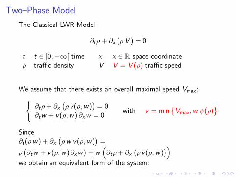
We assume that there exists an overall maximal speed Vmax:{∂tρ+ ∂x
(ρ v(ρ,w)
)= 0
∂tw + v(ρ,w) ∂xw = 0with v = min
{Vmax,w ψ(ρ)
}
Two–Phase Model
The Classical LWR Model
∂tρ+ ∂x (ρV ) = 0
t t ∈ [0,+∞[ time x x ∈ R space coordinateρ traffic density V V = V (ρ) traffic speed
We assume that there exists an overall maximal speed Vmax:{∂tρ+ ∂x
(ρ v(ρ,w)
)= 0
∂tw + v(ρ,w) ∂xw = 0with v = min
{Vmax,w ψ(ρ)
}Since∂t(ρw) + ∂x
(ρw v(ρ,w)
)=
ρ(∂tw + v(ρ,w) ∂xw
)+ w
(∂tρ+ ∂x
(ρ v(ρ,w)
))we obtain an equivalent form of the system:

Two–Phase Model
The Classical LWR Model
∂tρ+ ∂x (ρV ) = 0
t t ∈ [0,+∞[ time x x ∈ R space coordinateρ traffic density V V = V (ρ) traffic speed
A 2× 2 system of conservation laws with a C0,1 flow:{∂tρ+ ∂x
(ρ v(ρ,w)
)= 0
∂t(ρw) + ∂x(ρw v(ρ,w)
)= 0
with v = min{
Vmax,w ψ(ρ)}
Two–Phase Model
The Classical LWR Model
∂tρ+ ∂x (ρV ) = 0
t t ∈ [0,+∞[ time x x ∈ R space coordinateρ traffic density V V = V (ρ) traffic speed
A 2× 2 system of conservation laws with a C0,1 flow:{∂tρ+ ∂x
(ρ v(ρ,w)
)= 0
∂t(ρw) + ∂x(ρw v(ρ,w)
)= 0
with v = min{
Vmax,w ψ(ρ)}
S. Blandin, D. Work, P. Goatin, B. Piccoli, A. Bayen: SIAM J.Appl.Math. 2011
R.M. Colombo, F. Marcellini, M. Rascle: SIAM J.Appl.Math. 2010

Two–Phase Model
The Classical LWR Model
∂tρ+ ∂x (ρV ) = 0
t t ∈ [0,+∞[ time x x ∈ R space coordinateρ traffic density V V = V (ρ) traffic speed
With η = ρw :{∂tρ+ ∂x
(ρ v(ρ,w)
)= 0
∂tη + ∂x(η v(ρ, η)
)= 0
with v = min
{Vmax,
η
ρψ(ρ)
}

Two–Phase Model
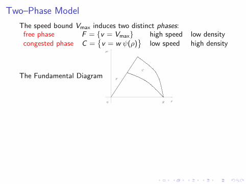
The speed bound Vmax induces two distinct phases:free phase F = {v = Vmax} high speed low densitycongested phase C =
{v = w ψ(ρ)
}low speed high density
The Fundamental Diagram
0
ρv
ρR
F
C
0
w
ρR
F
C
Vmax
w
w
0
η
ρR
F
C
Two–Phase Model
The speed bound Vmax induces two distinct phases:free phase F = {v = Vmax} high speed low densitycongested phase C =
{v = w ψ(ρ)
}low speed high density
The Fundamental Diagram
0
ρv
ρR
F
C
0
w
ρR
F
C
Vmax
w
w
0
η
ρR
F
C

Two–Phase Model
The speed bound Vmax induces two distinct phases:free phase F = {v = Vmax} high speed low densitycongested phase C =
{v = w ψ(ρ)
}low speed high density
The Fundamental Diagram
0
ρv
ρR
F
C
0
w
ρR
F
C
Vmax
w
w
0
η
ρR
F
C

Two–Phase Model – The Riemann Problem
For all states (ρl , ηl), (ρr , ηr ) ∈ F ∪ C , the Riemann problem of{∂tρ+ ∂x
(ρ v(ρ, η)
)= 0
∂tη + ∂x(η v(ρ, η)
)= 0
with v(ρ, η) = min
{Vmax,
η
ρψ(ρ)
}with initial data
ρ(0, x) =
{ρl if x < 0ρr if x > 0
η(0, x) =
{ηl if x < 0ηr if x > 0
Theorem (R.M.Colombo, F.Marcellini, M.Rascle: SIAM J.Appl.Math. 2010)
The Riemann problem admits a unique self similar weak entropysolution (ρ, η)

Two–Phase Model – The Riemann Problem
For all states (ρl , ηl), (ρr , ηr ) ∈ F ∪ C , the Riemann problem of{∂tρ+ ∂x
(ρ v(ρ, η)
)= 0
∂tη + ∂x(η v(ρ, η)
)= 0
with v(ρ, η) = min
{Vmax,
η
ρψ(ρ)
}with initial data
ρ(0, x) =
{ρl if x < 0ρr if x > 0
η(0, x) =
{ηl if x < 0ηr if x > 0
If(ρl , ηl) ∈ F (ρr , ηr ) ∈ C(ρl , ηl) ∈ C (ρr , ηr ) ∈ F
}⇒ Phase Transitions

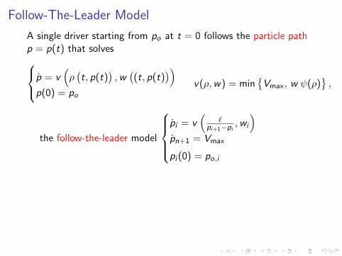
Follow-The-Leader Model
A single driver starting from po at t = 0 follows the particle pathp = p(t) that solvesp = v
(ρ(t, p(t)
),w((t, p(t)
))p(0) = po
v(ρ,w) = min{
Vmax, w ψ(ρ)},

Follow-The-Leader Model
A single driver starting from po at t = 0 follows the particle pathp = p(t) that solvesp = v
(ρ(t, p(t)
),w((t, p(t)
))p(0) = po
v(ρ,w) = min{
Vmax, w ψ(ρ)},
w is specific of every single driver, w(t, p(t)
)= w(0, po)

Follow-The-Leader Model
A single driver starting from po at t = 0 follows the particle pathp = p(t) that solvesp = v
(ρ(t, p(t)
),w((t, p(t)
))p(0) = po
v(ρ,w) = min{
Vmax, w ψ(ρ)},
w is specific of every single driver, w(t, p(t)
)= w(0, po)
n drivers, ` standard car length
⇒ ρ(t, x) '∑i
`
pi+1(t)− pi (t)χ]pi (t),pi+1(t)](x)
Follow-The-Leader Model
A single driver starting from po at t = 0 follows the particle pathp = p(t) that solvesp = v
(ρ(t, p(t)
),w((t, p(t)
))p(0) = po
v(ρ,w) = min{
Vmax, w ψ(ρ)},
If
the follow-the-leader model
pi = v
(`
pi+1−pi ,wi
)pn+1 = Vmax
pi (0) = po,i
is such that
∑i
`
pi+1(t)− pi (t)χ]pi (t),pi+1(t)](x)→ ρ(t, x) a.e.
then ρ solves the macroscopic model.

Follow-The-Leader Model
A single driver starting from po at t = 0 follows the particle pathp = p(t) that solvesp = v
(ρ(t, p(t)
),w((t, p(t)
))p(0) = po
v(ρ,w) = min{
Vmax, w ψ(ρ)},
If the follow-the-leader model
pi = v
(`
pi+1−pi ,wi
)pn+1 = Vmax
pi (0) = po,i
is such that
∑i
`
pi+1(t)− pi (t)χ]pi (t),pi+1(t)](x)→ ρ(t, x) a.e.
then ρ solves the macroscopic model.

Follow-The-Leader Model
Scheme
(ρ, w)
→
(ρ(t),w(t)
)
discretize
↓ ↑
n→ +∞
(pni , w
ni ) →
(pni (t),wn
i (t))
Cauchy Theorem

Follow-The-Leader Model
Scheme
(ρ, w)
→
(ρ(t),w(t)
)discretize ↓ ↑
n→ +∞
(pni , w
ni ) →
(pni (t),wn
i (t))
Cauchy Theorem

Follow-The-Leader Model
Scheme
(ρ, w)
→
(ρ(t),w(t)
)discretize ↓ ↑
n→ +∞
(pni , w
ni ) →
(pni (t),wn
i (t))
Cauchy Theorem

Follow-The-Leader Model
Scheme
(ρ, w)
→
(ρ(t),w(t)
)discretize ↓ ↑ n→ +∞
(pni , w
ni ) →
(pni (t),wn
i (t))
Cauchy Theorem

Follow-The-Leader Model
Scheme
(ρ, w) →(ρ(t),w(t)
)discretize ↓ ↑ n→ +∞
(pni , w
ni ) →
(pni (t),wn
i (t))
Cauchy Theorem

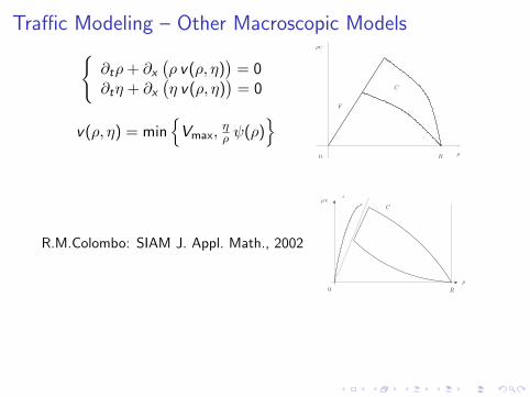
Traffic Modeling – Other Macroscopic Models{∂tρ+ ∂x
(ρ v(ρ, η)
)= 0
∂tη + ∂x(η v(ρ, η)
)= 0
v(ρ, η) = min{
Vmax,ηρ ψ(ρ)
}
0
ρv
ρR
F
C
I J.P.Lebacque, S.Mammar, H.Haj Salem: ISTTT, 2007

Traffic Modeling – Other Macroscopic Models{∂tρ+ ∂x
(ρ v(ρ, η)
)= 0
∂tη + ∂x(η v(ρ, η)
)= 0
v(ρ, η) = min{
Vmax,ηρ ψ(ρ)
}
0
ρv
ρR
F
C
I A.Aw, M.Rascle: SIAM J.Appl.Math., 2000
I M.Zhang: Transportation Research, 2002
I P.Goatin: Math. Comput. Modelling, 2006{∂tρ+ ∂x
[ρ v(ρ, y)
]= 0
∂ty + ∂x[y v(ρ, y)
]= 0
v(ρ, y) = yρ − p(ρ)
I J.P.Lebacque, S.Mammar, H.Haj Salem: ISTTT, 2007

Traffic Modeling – Other Macroscopic Models{∂tρ+ ∂x
(ρ v(ρ, η)
)= 0
∂tη + ∂x(η v(ρ, η)
)= 0
v(ρ, η) = min{
Vmax,ηρ ψ(ρ)
}0
ρv
ρR
F
C
I A.Aw, M.Rascle: SIAM J.Appl.Math., 2000
I M.Zhang: Transportation Research, 2002
I P.Goatin: Math. Comput. Modelling, 2006{∂tρ+ ∂x
[ρ v(ρ, y)
]= 0
∂ty + ∂x[y v(ρ, y)
]= 0
v(ρ, y) = yρ − p(ρ)
ρ v
0 R
ρ
I J.P.Lebacque, S.Mammar, H.Haj Salem: ISTTT, 2007

Traffic Modeling – Other Macroscopic Models{∂tρ+ ∂x
(ρ v(ρ, η)
)= 0
∂tη + ∂x(η v(ρ, η)
)= 0
v(ρ, η) = min{
Vmax,ηρ ψ(ρ)
}0
ρv
ρR
F
C
R.M.Colombo: SIAM J. Appl. Math., 2002
Free flow: (ρ, q) ∈ F , Congested flow: (ρ, q) ∈ C ,
∂tρ+ ∂x[ρ · vF (ρ)
]= 0,
{∂tρ+ ∂x
[ρ · vC (ρ, q)
]= 0
∂tq + ∂x[(q − q∗) · vC (ρ, q)
]= 0
vF (ρ) =(1− ρ
R
)· V vC (ρ, q) =
(1− ρ
R
)· qρ
I J.P.Lebacque, S.Mammar, H.Haj Salem: ISTTT, 2007
Traffic Modeling – Other Macroscopic Models{∂tρ+ ∂x
(ρ v(ρ, η)
)= 0
∂tη + ∂x(η v(ρ, η)
)= 0
v(ρ, η) = min{
Vmax,ηρ ψ(ρ)
}0
ρv
ρR
F
C
R.M.Colombo: SIAM J. Appl. Math., 2002
ρ v
0 R
ρ
F
C
I J.P.Lebacque, S.Mammar, H.Haj Salem: ISTTT, 2007

Traffic Modeling – Other Macroscopic Models{∂tρ+ ∂x
(ρ v(ρ, η)
)= 0
∂tη + ∂x(η v(ρ, η)
)= 0
v(ρ, η) = min{
Vmax,ηρ ψ(ρ)
}0
ρv
ρR
F
C
R.M.Colombo: SIAM J. Appl. Math., 2002
ρ v
0 R
ρ
F
C
I J.P.Lebacque, S.Mammar, H.Haj Salem: ISTTT, 2007

A Kinetic Model{∂tρ+ ∂x
(ρ v(ρ, η)
)= 0
∂tη + ∂x(η v(ρ, η)
)= 0
v(ρ, η) = min{
Vmax,ηρ ψ(ρ)
}S.Benzoni-Gavage, R.M.Colombo, P.Gwiazda: Proc. R. Soc. London, 2006
∂tr(t, x ; w) + ∂x
w r(t, x ; w)ψ
(∫ w
wr(t, x ; w ′) dw ′
) = 0 .
The unknown r = r(t, x ,w) is the probability density of vehicleshaving maximal speed w that at time t are at point x

A Kinetic Model{∂tρ+ ∂x
(ρ v(ρ, η)
)= 0
∂tη + ∂x(η v(ρ, η)
)= 0
v(ρ, η) = min{
Vmax,ηρ ψ(ρ)
}S.Benzoni-Gavage, R.M.Colombo, P.Gwiazda: Proc. R. Soc. London, 2006
∂tr(t, x ; w) + ∂x
w r(t, x ; w)ψ
(∫ w
wr(t, x ; w ′) dw ′
) = 0 .
If the measure r solves the kinetic model and is such that
r(t, x ; ·) = ρ(t, x) δw(t,x)
than (ρ,w) solves the 2−phase model

Experimental Fundamental Diagrams
B.Kerner K.M.Kockelman
Traffic and Granular Flow Transportation, 2001
Springer Verlag, 2000

Experimental Fundamental Diagrams
B.Kerner K.M.Kockelman
Traffic and Granular Flow Transportation, 2001
Springer Verlag, 2000
0
ρv
ρR
F
CFundamental Diagram byR.M. Colombo, F. Marcellini, M. Rascle
SIAM J. Appl. Math. 2010

Discrete–Continuous Description
The Macroscopic Part: LWR Model
∂tρ+ ∂x (ρ v) = 0
t t ∈ [0,+∞[ time x x ∈ R space coordinateρ traffic density v v = v(ρ) traffic speed
The Microscopic Part: Follow-the-Leader Model
pi = v
(`
pi+1 − pi
)pi = pi (t) position of the i−th driver, for i = 1, ..., n` > 0 vehicles’ lenght and
pi+1 − pi ≥ `

Discrete–Continuous Description
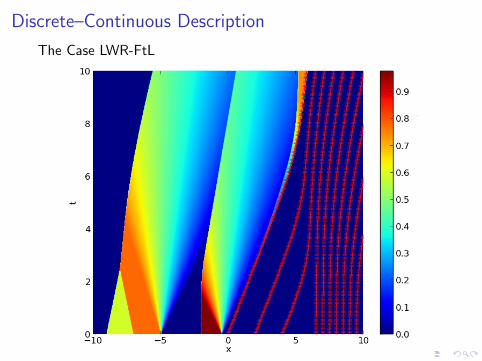
The Case LWR-FtL
∂tρ+ ∂x(ρ v(ρ)
)= 0 x < p1(t)
pi = v(
`pi+1−pi
)i = 1, . . . , n − 1
pn = w(t)ρ(0, x) = ρ(x) x ≤ p1
p(0) = p
Theorem (R.M. Colombo, F. Marcellini: Math. Meth. Appl. Sci., 2014)

Discrete–Continuous Description
The Case LWR-FtL
∂tρ+ ∂x(ρ v(ρ)
)= 0 x < p1(t)
pi = v(
`pi+1−pi
)i = 1, . . . , n − 1
pn = w(t)ρ(0, x) = ρ(x) x ≤ p1
p(0) = p
Theorem (R.M. Colombo, F. Marcellini: Math. Meth. Appl. Sci., 2014)
There exists a unique solution (ρ, p) such that
ρ ∈ C0(
[0,T ]; (L1 ∩ BV)(R; [0, 1]))
ρ(t, x) = 0 for x > p1(t)
p ∈ W1,∞([0,T ];Rn)

Discrete–Continuous Description
The Case LWR-FtL
∂tρ+ ∂x(ρ v(ρ)
)= 0 x < p1(t)
pi = v(
`pi+1−pi
)i = 1, . . . , n − 1
pn = w(t)ρ(0, x) = ρ(x) x ≤ p1
p(0) = p
Theorem (R.M. Colombo, F. Marcellini: Math. Meth. Appl. Sci., 2014)
There exists a constant C > 0 such that∥∥∥ρ(t) − ρ′(t)∥∥∥L1
≤ C∥∥∥ρ− ρ′
∥∥∥L1
+ C(1 + t)
[∥∥∥p − p′∥∥∥ +
∥∥∥w − w ′∥∥∥L1([0,t])
]e2
Lip(v)`
t
∥∥∥p(t) − p′(t)∥∥∥ ≤
[∥∥∥p − p′∥∥∥ +
∥∥∥w − w ′∥∥∥L1([0,t])
]e2
Lip(v)`
t .

Discrete–Continuous Description
The Case FtL-LWR
∂tρ+ ∂x(ρ v(ρ)
)= 0 x > pn(t)
pi = v(
`pi+1−pi
)i = 1, . . . , n − 1
pn = v(ρ(t, pn(t))
)ρ(0, x) = ρ(x) x ≥ pn
p(0) = p
I Well posedness result as before
I Extension to FtL – LWR – FtL – LWR . . .
I With fixed boundary and micro-macro transitionsC. Lattanzio, B. Piccoli: Math. Mod. Meth. Appl. Sci., 2010
Discrete–Continuous Description
The Case LWR-FtL

Discrete–Continuous Description
The Case FtL-LWR
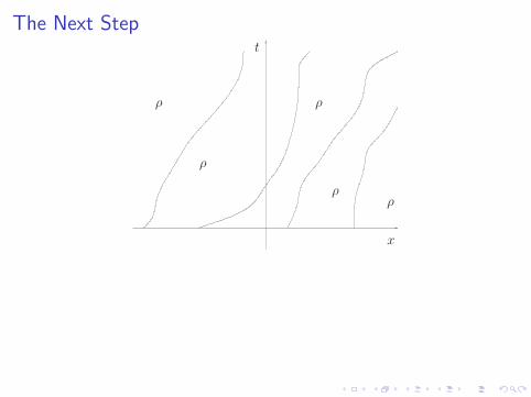
The Next Step
x
t
ρ
ρ
ρ
ρ
ρ

The Next Step
x
t
ρ
ρ
ρ
ρ
ρ
I Millennium Project
I D.B. Work, S. Blandin, O. Tossavainen, B. Piccoli, A. Bayen: Appl.
Math. Res. Express, 2010
I C. Lattanzio, A. Maurizi, B. Piccoli: SIAM J. Math. Anal., 2011
I A. Cabassi, P. Goatin: Res. Report INRIA, 2013

The Next Step
x
t
ρ
ρ
ρ
ρ
ρ
I A. Alessandri, R. Bolla, M. Repetto: Proc. Amer. Control Conf.,
2003
I P. Cheng, Z. Qiu, B. Ran: Proc. IEEE ITSC’06, 2006
I J.-C. Herrera, D. Work, R. Herring, J.Ban, Q. Jacobson, A. Bayen:
Transp. Res. C, 2009

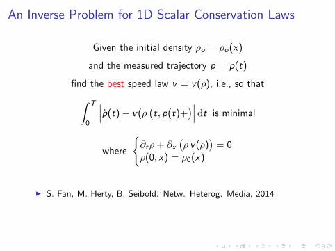
An Inverse Problem for 1D Scalar Conservation Laws
Given the initial density ρo = ρo(x)
and the measured trajectory p = p(t)
find the best speed law v = v(ρ), i.e., so that∫ T
0
∣∣∣p(t)− v(ρ(t, p(t)+
)∣∣∣ dt is minimal
where
{∂tρ+ ∂x
(ρ v(ρ)
)= 0
ρ(0, x) = ρ0(x)
I S. Fan, M. Herty, B. Seibold: Netw. Heterog. Media, 2014
A solution may fail to exist

Inverse Problem – A Negative Example
Class of speed laws: vε(ρ) = (1 + ερ)(1− ρ)
ρ1
1
0
v
ρ1
1
0
v
ρ1
1
0
v

Inverse Problem – A Negative Example
Class of speed laws: vε(ρ) = (1 + ερ)(1− ρ)
Measured trajectory: p(t) = t/2
ρε solves:
∂tρ+ ∂x
(ρ v(ρ)
)= 0
ρ(0, x) =
{1/8 x < 03/8 x > 0

Inverse Problem – A Negative Example
Class of speed laws: vε(ρ) = (1 + ερ)(1− ρ)
Measured trajectory: p(t) = t/2
ρε solves:
∂tρ+ ∂x
(ρ v(ρ)
)= 0
ρ(0, x) =
{1/8 x < 03/8 x > 0
ϕ : [−1/3, 1/3] → R
ε →∫ T
0
∣∣∣∣p(t)− vε(ρε(t, p(t)+
))∣∣∣∣dt
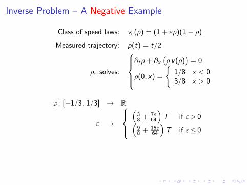
Inverse Problem – A Negative Example
Class of speed laws: vε(ρ) = (1 + ερ)(1− ρ)
Measured trajectory: p(t) = t/2
ρε solves:
∂tρ+ ∂x
(ρ v(ρ)
)= 0
ρ(0, x) =
{1/8 x < 03/8 x > 0
ϕ : [−1/3, 1/3] → R
ε →
(
38 + 7ε
64
)T if ε> 0(
98 + 15ε
64
)T if ε≤ 0

Inverse Problem – A Negative Example
Class of speed laws: vε(ρ) = (1 + ερ)(1− ρ)
Measured trajectory: p(t) = t/2
ρε solves:
∂tρ+ ∂x
(ρ v(ρ)
)= 0
ρ(0, x) =
{1/8 x < 03/8 x > 0
ε
ϕ

Inverse Problem – A Positive Result
Class of Speed Laws: vV (ρ) = V (1− ρ) for V ∈ [V , V ].
ρ10
v
V
ρ10
vV
ρ10
v
V

Inverse Problem – A Positive Result
Class of Speed Laws: vV (ρ) = V (1− ρ) for V ∈ [V , V ].
Theorem (R.M.Colombo, F.Marcellini: Math. Mod. Meth. Appl. Sci.,2015)
Let ρo ∈ (L1 ∩ BV)(R; [0, 1]) and p ∈W1,∞([0,T ];R).
Let ρV solve
{∂tρV + ∂x
(V ρV (1− ρV )
)= 0
ρV (0, x) = ρo(x) .
Then, the map
ϕ : [V , V ] → R
V →∫ T
0
∣∣∣∣p(t)− vV
(ρV(t, p(t)+
))∣∣∣∣ dt
is continuous, provided
essinfx∈R ρo > ρ and essinft∈[0,T ] p ≥ V (1− 2ρ) .

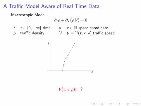
A Traffic Model Aware of Real Time Data
Macroscopic Model∂tρ+ ∂x (ρV) = 0
t t ∈ [0,+∞[ time x x ∈ R space coordinateρ traffic density V V = V(t, x , ρ) traffic speed

A Traffic Model Aware of Real Time Data
Macroscopic Model∂tρ+ ∂x (ρV) = 0
t t ∈ [0,+∞[ time x x ∈ R space coordinateρ traffic density V V = V(t, x , ρ) traffic speed
A Traffic Model Aware of Real Time Data
Macroscopic Model∂tρ+ ∂x (ρV) = 0
t t ∈ [0,+∞[ time x x ∈ R space coordinateρ traffic density V V = V(t, x , ρ) traffic speed
x
t
V(t, x , ρ) = ?

A Traffic Model Aware of Real Time Data
Macroscopic Model∂tρ+ ∂x (ρV) = 0
t t ∈ [0,+∞[ time x x ∈ R space coordinateρ traffic density V V = V(t, x , ρ) traffic speed
x
t
V(t, x , ρ) = ?

A Traffic Model Aware of Real Time Data
Macroscopic Model∂tρ+ ∂x (ρV) = 0
t t ∈ [0,+∞[ time x x ∈ R space coordinateρ traffic density V V = V(t, x , ρ) traffic speed
x
t
V(t, x , ρ) = v(ρ)

A Traffic Model Aware of Real Time Data
Macroscopic Model∂tρ+ ∂x (ρV) = 0
t t ∈ [0,+∞[ time x x ∈ R space coordinateρ traffic density V V = V(t, x , ρ) traffic speed
x
t
V(t, x , ρ) =2
1p(t) + 1
v(ρ)

A Traffic Model Aware of Real Time Data
Macroscopic Model∂tρ+ ∂x (ρV) = 0
t t ∈ [0,+∞[ time x x ∈ R space coordinateρ traffic density V V = V(t, x , ρ) traffic speed
x
t
V(t, x , ρ) = χ(x − p(t)
) 21
p(t) + 1v(ρ)
+(
1− χ(x − p(t)
))v(ρ)

A Traffic Model Aware of Real Time Data
Theorem (R.M.Colombo, F.Marcellini: Math. Mod. Meth. Appl. Sci.,2015)
The Cauchy Problem∂tρ+ ∂x
(ρV(t, x , ρ)
)= 0
V(t, x , ρ) = χ(x − p(t)
) 2p(t) v(ρ)p(t)+v(ρ) +
(1− χ
(x − p(t)
))v(ρ)
ρ(0, x) = ρo(x)
admits a unique solution.
I E.Y. Panov: Arch. Rat. Mech. An., 2010
I K.H. Karlsen, N.H. Risebro: Discr. Cont. Dyn. Syst. – A, 2003
I B. Andreianov, P. Benilan, S.N. Kruzkov: J. Func. An., 2000

A Traffic Model Aware of Real Time Data