Counting - WordPress.com · Let examine the informal idea Enumerating rows in increasing order is...
32
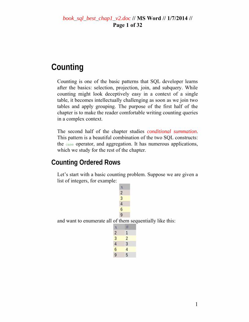
book_sql_best_chap1_v2.doc // MS Word // 1/7/2014 // Page 1 of 32 1 Counting Counting is one of the basic patterns that SQL developer learns after the basics: selection, projection, join, and subquery. While counting might look deceptively easy in a context of a single table, it becomes intellectually challenging as soon as we join two tables and apply grouping. The purpose of the first half of the chapter is to make the reader comfortable writing counting queries in a complex context. The second half of the chapter studies conditional summation. This pattern is a beautiful combination of the two SQL constructs: the case operator, and aggregation. It has numerous applications, which we study for the rest of the chapter. Counting Ordered Rows Let’s start with a basic counting problem. Suppose we are given a list of integers, for example: x 2 3 4 6 9 and want to enumerate all of them sequentially like this: x # 2 1 3 2 4 3 6 4 9 5 1
Transcript of Counting - WordPress.com · Let examine the informal idea Enumerating rows in increasing order is...
book_sql_best_chap1_v2.doc // MS Word // 1/7/2014 //Page 1 of 32
1Counting
Counting is one of the basic patterns that SQL developer learnsafter the basics: selection, projection, join, and subquery. Whilecounting might look deceptively easy in a context of a singletable, it becomes intellectually challenging as soon as we join twotables and apply grouping. The purpose of the first half of thechapter is to make the reader comfortable writing counting queriesin a complex context.
The second half of the chapter studies conditional summation.This pattern is a beautiful combination of the two SQL constructs:the case operator, and aggregation. It has numerous applications,which we study for the rest of the chapter.
Counting Ordered Rows
Let’s start with a basic counting problem. Suppose we are given alist of integers, for example:
x 2 3 4 6 9
and want to enumerate all of them sequentially like this: x # 2 1 3 2 4 3 6 4 9 5
1

book_sql_best_chap1_v2.doc // MS Word // 1/7/2014 //Page 2 of 32
Enumerating rows in the increasing order is the same as countinghow many rows precede a given row.
SQL enjoys success unparalleled by any rival query language. Notthe last reason for such popularity might be credited to itsproximity to English1. Let examine the informal ideaEnumerating rows in increasing order is counting how many rows precede a given row.
carefully. Perhaps the most important is that we referred to therows in the source table twice: first, to a given row, second, to apreceding row. Therefore, we need to join our number list withitself (fig 1.1).
Cartesian Product
Surprisingly, not many basic SQL tutorials, which are so abundant on the web today, mention Cartesian product. Cartesian product is a join operator with no join condition2 select A.*, B.* from A, B
1 This proximity partially explains why newer relational languages had such a limited success. For for example, Tutorial D has succinct notation, better NULL handling, and pure set semantics. These are not breakthrough features however; a New and Improved query language had better be leaps and bounds ahead, not just simpler to type.
2 Many DBAs would jump in pointing that queries with Cartesian product are inefficient, but the rule of thumb avoiding Cartesian product is just too simplistic.
2

book_sql_best_chap1_v2.doc // MS Word // 1/7/2014 //Page 3 of 32
Figure 1.1: Cartesian product of the set A = {2,3,4,6,9} by itself.Counting all the elements x that are no greater than y produces thesequence number of y in the set A.
Carrying over this idea into formal SQL query is straightforward.As it is our first query in this book, let’s do it step by step. TheCartesian product itself isselect t.x x, tt.x y3 from T t, T tt
Next, the triangle area below the main diagonal isselect t.x x, tt.x yfrom T t, T ttwhere tt.x <= t.x
Finally, we need only one column – t.x – which we group theprevious result by and countselect t.x, count(*) seqNum from T t, T ttwhere tt.x <= t.x group by t.x
3 We use Oracle syntax and write <column expr> <alias> instead of ANSI SQL <columnexpr> AS <alias>. Ditto for table expressions.
3
2
3
4
6
9
2 3 4 6 9
y
x
1
2
3
4
5

book_sql_best_chap1_v2.doc // MS Word // 1/7/2014 //Page 4 of 32
What if we modify the problem slightly and ask for a list of pairswhere each number is coupled with its predecessor?
x predecessor 2 3 2 4 3 6 4 9 6
Let me provide a typical mathematician’s answer, first -- it isremarkable in a certain way. Given that we already know how tonumber list elements successively, it might be tempted to reducethe current problem to the previous one:Enumerate all the numbers in the increasing order and match each sequence number seq#with predecessor seq#-1. Next!
This attitude is, undoubtedly, the most economical way ofthinking, although not necessarily producing the most efficientSQL. Therefore, let’s revisit our original approach, as illustratedon fig 1.2.
Equivalence Relation and Group By
Almost any other SQL query uses group by operator. Why is groupby operator so powerful? It is not among the fundamental relational algebra operators. A partial answer to this fascinatingefficiency is that group by embodies an equivalence relation. Indeed, it partitions rows into equivalence classes of rows with identical values in a column or a group of columns, and calculates aggregate values per each equivalence class.
4
book_sql_best_chap1_v2.doc // MS Word // 1/7/2014 //Page 5 of 32
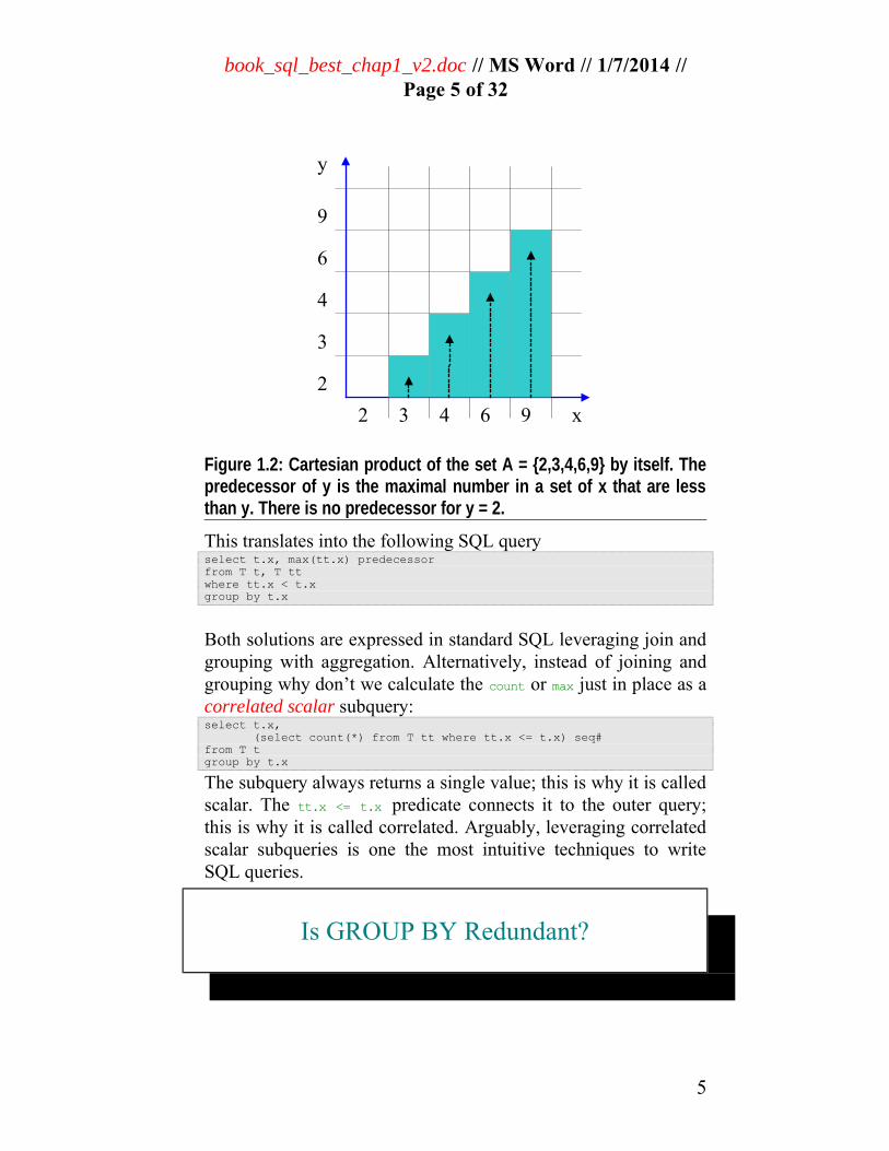
Figure 1.2: Cartesian product of the set A = {2,3,4,6,9} by itself. Thepredecessor of y is the maximal number in a set of x that are lessthan y. There is no predecessor for y = 2.
This translates into the following SQL query select t.x, max(tt.x) predecessor from T t, T ttwhere tt.x < t.x group by t.x
Both solutions are expressed in standard SQL leveraging join andgrouping with aggregation. Alternatively, instead of joining andgrouping why don’t we calculate the count or max just in place as acorrelated scalar subquery: select t.x, (select count(*) from T tt where tt.x <= t.x) seq# from T t group by t.x
The subquery always returns a single value; this is why it is calledscalar. The tt.x <= t.x predicate connects it to the outer query;this is why it is called correlated. Arguably, leveraging correlatedscalar subqueries is one the most intuitive techniques to writeSQL queries.
Is GROUP BY Redundant?
5
2
3
4
6
9
2 3 4 6 9
y
x
book_sql_best_chap1_v2.doc // MS Word // 1/7/2014 //Page 6 of 32
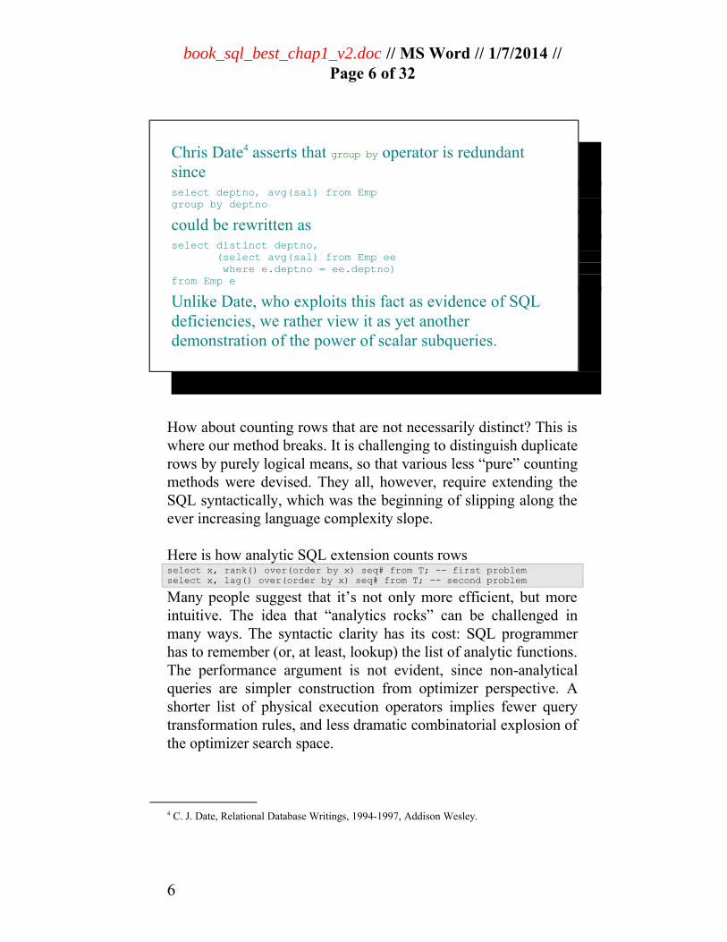
Chris Date4 asserts that group by operator is redundant since select deptno, avg(sal) from Empgroup by deptno
could be rewritten as select distinct deptno, (select avg(sal) from Emp ee where e.deptno = ee.deptno)from Emp e
Unlike Date, who exploits this fact as evidence of SQL deficiencies, we rather view it as yet another demonstration of the power of scalar subqueries.
How about counting rows that are not necessarily distinct? This iswhere our method breaks. It is challenging to distinguish duplicaterows by purely logical means, so that various less “pure” countingmethods were devised. They all, however, require extending theSQL syntactically, which was the beginning of slipping along theever increasing language complexity slope.
Here is how analytic SQL extension counts rows select x, rank() over(order by x) seq# from T; -- first problemselect x, lag() over(order by x) seq# from T; -- second problem
Many people suggest that it’s not only more efficient, but moreintuitive. The idea that “analytics rocks” can be challenged inmany ways. The syntactic clarity has its cost: SQL programmerhas to remember (or, at least, lookup) the list of analytic functions.The performance argument is not evident, since non-analyticalqueries are simpler construction from optimizer perspective. Ashorter list of physical execution operators implies fewer querytransformation rules, and less dramatic combinatorial explosion ofthe optimizer search space.
4 C. J. Date, Relational Database Writings, 1994-1997, Addison Wesley.
6

book_sql_best_chap1_v2.doc // MS Word // 1/7/2014 //Page 7 of 32
It might even be argued that the syntax could be better. Thepartition by and order by clauses have similar functionality to thegroup by and order by clauses in the main query block. Yet onename was reused, and the other had been chosen to have a newname. Unlike other scalar expressions, which can be placedanywhere in SQL query where scalar values are accepted, theanalytics clause lives in the scope of the select clause only. I havenever been able to suppress an impression that analytic extensioncould be designed in more natural way.
Conditional Summation with CASE operator
The genesis of the conditional summation idiom is an equivalencebetween the count(*) and sum(1). Formally, select count(*) from emp
is the same as select sum(1) from emp
Before elevating this observation into the main topic of thissection – the conditional summation pattern – let’s clarify onepeculiar detail about the syntax. It's just a misconception that countshould have any arguments at all. First, for most practicalpurposes count = sum(1), and there is no free variable parameterwithin the sum(1) expression. Second, think how the count functionmay be implemented on a low-level. A reasonable code must looklike this int count = 0;for( int i = 0; i< 10; i++) count = count + 1;
The count variable is updated during each row processing with theunary increment operator +1. Unlike the count, any "normal"aggregation has to use a binary operation during each aggregateincremental computation stepint sum = 0;for( int i = 0; i< 10; i++) sum = sum + element[i];
that is, + for sum, ∨ for max, ∧ for min, etc. Therefore, we need oneargument for normal aggregates, and no arguments for the count.
7
book_sql_best_chap1_v2.doc // MS Word // 1/7/2014 //Page 8 of 32
OK, as far as simple counting is concerned, there doesn’t appearto be any need for an argument. But what about select count(ename) from emp
where only non-null values of the ename column are counted? Thedescription of the count(ename) in the previous sentence translatesdirectly into SQLselect count(*) from emp where ename is not null
We see that count(ename) is no more than a syntax shortcut.
Well, how about select count(distinct ename) from emp
where the count aggregate function accepts a column expressionwith a keyword? This is just yet another shortcutselect count(*) from ( select distinct empno from emp)
Argument for the COUNT
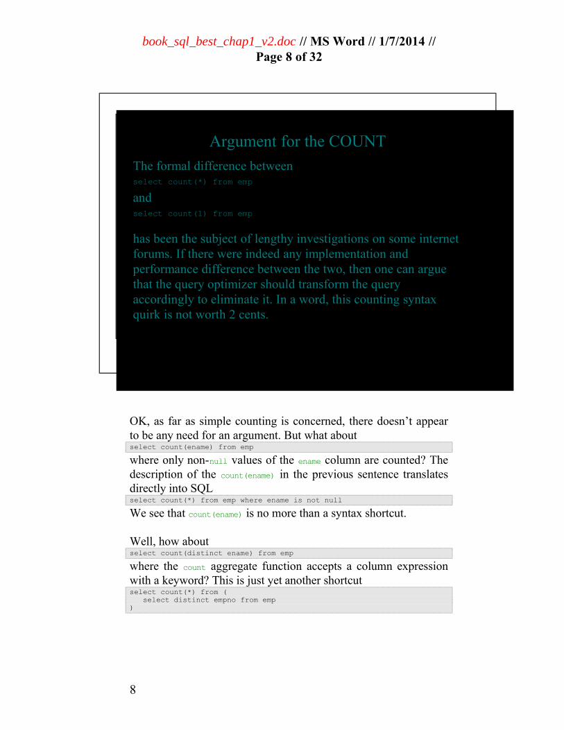
The formal difference between select count(*) from emp
and select count(1) from emp
has been the subject of lengthy investigations on some internet forums. If there were indeed any implementation and performance difference between the two, then one can argue that the query optimizer should transform the query accordingly to eliminate it. In a word, this counting syntax quirk is not worth 2 cents.
8
book_sql_best_chap1_v2.doc // MS Word // 1/7/2014 //Page 9 of 32
Next, what if we want to count two different values at the sametime like thisselect count(ename), count(*) from emp
Even though it looks like SQL has a dedicated syntax shortcut forevery imaginable task, at this point it is easy to argue that theseextensions are nifty at least in some practical cases.
Enter the conditional summation pattern. Whenever we countrows satisfying a certain criteria, e.g.select count(*) from empwhere sal < 1000
and feel that the where clause is an obstacle for the query to evolveto a more sophisticated form, we rewrite it without where clause select sum(case when sal < 1000 then 1 else 0 end)from emp
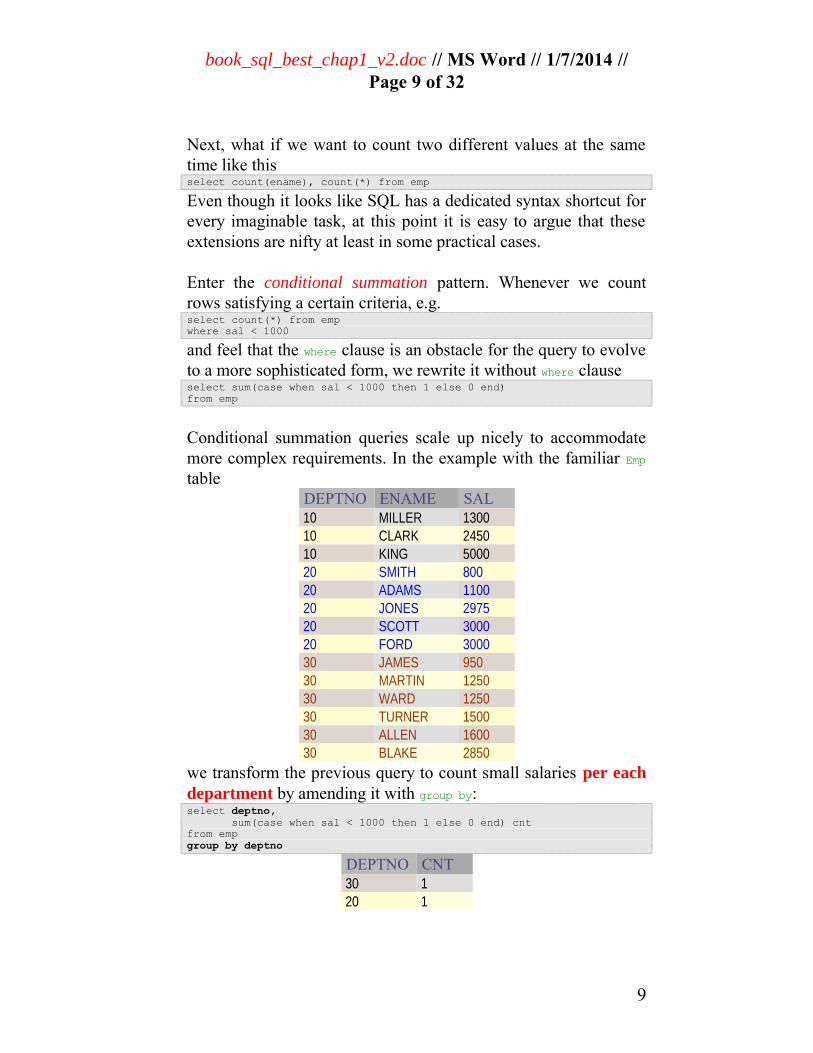
Conditional summation queries scale up nicely to accommodatemore complex requirements. In the example with the familiar Emptable
DEPTNO ENAME SAL 10 MILLER 1300 10 CLARK 2450 10 KING 5000 20 SMITH 800 20 ADAMS 1100 20 JONES 2975 20 SCOTT 3000 20 FORD 3000 30 JAMES 950 30 MARTIN 1250 30 WARD 1250 30 TURNER 1500 30 ALLEN 1600 30 BLAKE 2850
we transform the previous query to count small salaries per eachdepartment by amending it with group by: select deptno, sum(case when sal < 1000 then 1 else 0 end) cnt from empgroup by deptno
DEPTNO CNT 30 1 20 1
9

book_sql_best_chap1_v2.doc // MS Word // 1/7/2014 //Page 10 of 32
10 0 The subtle novelty here is that the conditional summation query isno longer equivalent to the former attempt restricting condition inthe where clauseselect deptno,count(*) from empwhere sal < 1000group by deptno
DEPTNO COUNT(*) 30 1 20 1
Zero counts were perfectly legal in the aggregation withoutgrouping case. Disappearing zeros are certainly a sign of (yetanother) SQL inconsistency.
Perhaps the most important rationalization for the conditionalsummation idiom is counting by different criteria. Without
Aggregation without Grouping
An aggregation with no grouping is, in fact, an aggregation within a single group. If SQL syntax allowed grouping by the empty set of columns ∅, then a simple aggregateselect count(*) from T
could be also represented asselect count(*) from Tgroup by ∅
Without the empty set syntax, we still can writeselect count(*) from Tgroup by 0
The 0 pseudo column is a constant expression, so that the table T is partitioned into a single group effectively the same way aswith the empty set.
10
book_sql_best_chap1_v2.doc // MS Word // 1/7/2014 //Page 11 of 32
conditional summation we would have to count by each individualcondition in a dedicated query block, and combine those countswith a join. The pivot operator, which would be studied in thechapter 3, is a typical showcase of this idea.
Before the case operator became widely available in the off-the-shelf RDBMS systems, much more ingenious counting methodwith indicator function was employed.
Indicator and Step Functions
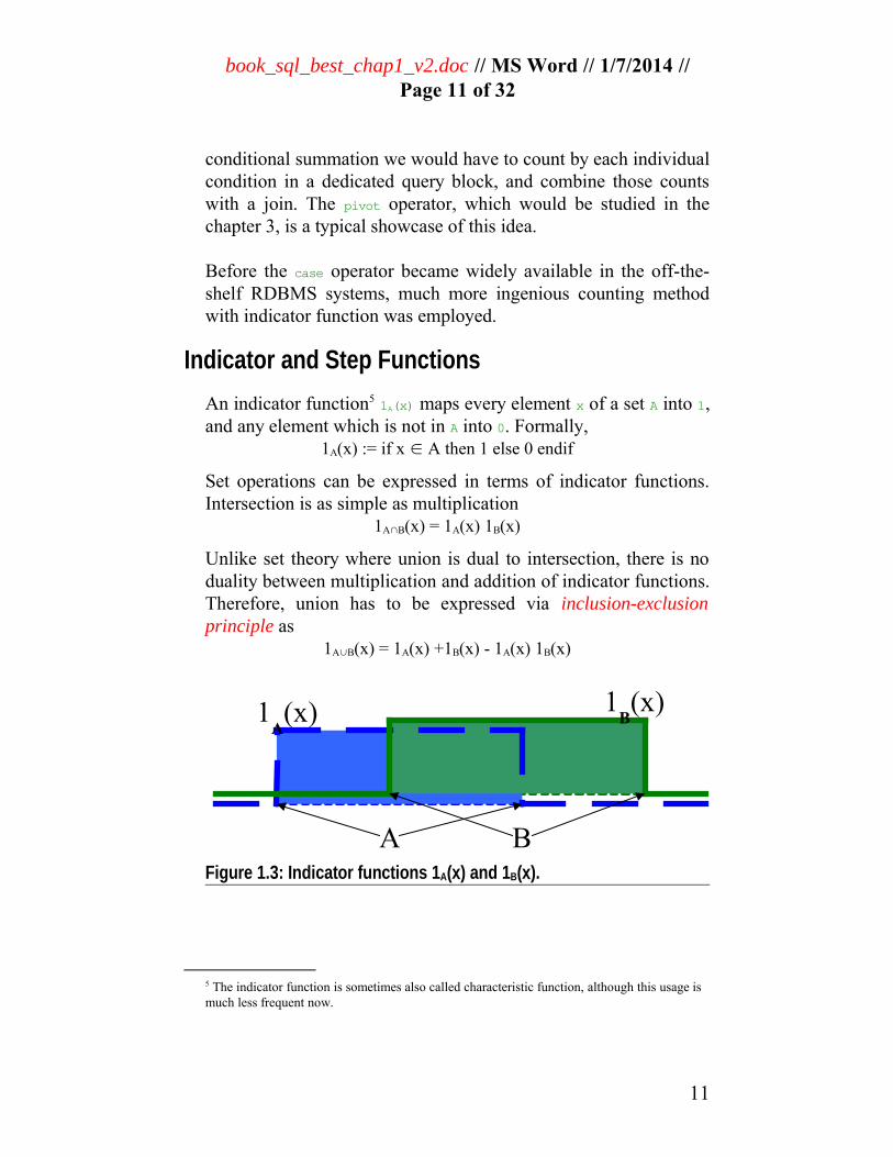
An indicator function5 1A(x) maps every element x of a set A into 1,and any element which is not in A into 0. Formally,
1A(x) := if x ∈ A then 1 else 0 endif
Set operations can be expressed in terms of indicator functions.Intersection is as simple as multiplication
1A∩B(x) = 1A(x) 1B(x)
Unlike set theory where union is dual to intersection, there is noduality between multiplication and addition of indicator functions.Therefore, union has to be expressed via inclusion-exclusionprinciple as
1A∪B(x) = 1A(x) +1B(x) - 1A(x) 1B(x)
Figure 1.3: Indicator functions 1A(x) and 1B(x).
5 The indicator function is sometimes also called characteristic function, although this usage is much less frequent now.
11
A B
1B(x)1
A(x)
book_sql_best_chap1_v2.doc // MS Word // 1/7/2014 //Page 12 of 32
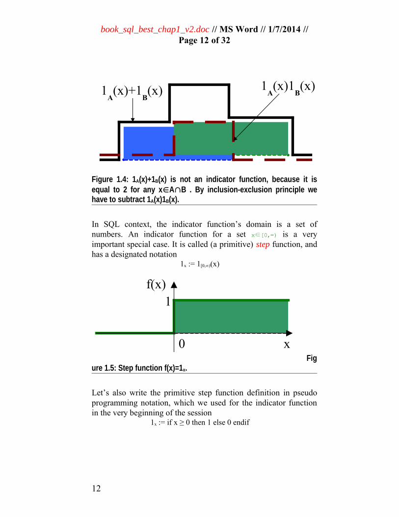
Figure 1.4: 1A(x)+1B(x) is not an indicator function, because it isequal to 2 for any x∈A∩B . By inclusion-exclusion principle wehave to subtract 1A(x)1B(x).
In SQL context, the indicator function’s domain is a set ofnumbers. An indicator function for a set x∈[0,∞) is a veryimportant special case. It is called (a primitive) step function, andhas a designated notation
1x := 1[0,∞)(x)
Figure 1.5: Step function f(x)=1x.
Let’s also write the primitive step function definition in pseudoprogramming notation, which we used for the indicator functionin the very beginning of the session
1x := if x ≥ 0 then 1 else 0 endif
12
0 x
1
1A(x)+1
B(x) 1
A(x)1
B(x)
f(x)
book_sql_best_chap1_v2.doc // MS Word // 1/7/2014 //Page 13 of 32
If we raise the abstraction level and convert these hardcodedconstants 0, 1 and yet another 0, into variables
if x ≥ x0 then α else β endif
then, our pseudo code starts looking similar to the case operator.This expression is a generic step function (although it doesn’thave abbreviated notation).
Generic step function can be expressed via primitive step functionif x ≥ x0 then α else β endif = α 1x-x0 + β 1 x0-x
So far, so good: we were able to handle simple case operators.What about nested case expressions? Consider
if x ≥ 0 then (if y ≥ 0 then 1 else 0 endif) else 0 endif
Easy: the above formula for general step function should handlethe case where α is an expression, rather than constant. Bysubstitution we have
if x ≥ 0 then (if y ≥ 0 then 1 else 0 endif) else 0 endif = 1y 1x
as if we had just an intersection of the x ≥ 0 and y ≥ 0 sets!
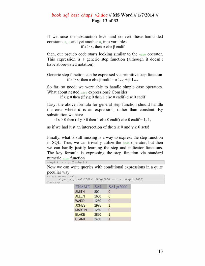
Finally, what is still missing is a way to express the step functionin SQL. True, we can trivially utilize the case operator, but thenwe can hardly justify learning the step and indicator functions.The key formula is expressing the step function via standardnumeric sign functionstep(x) := sign(1+sign(x))
Now we can write queries with conditional expressions in a quitepeculiar way select ename, sal, sign(1+sign(sal-2000)) SALgt2000 -- i.e. step(x-2000)from emp
ENAME SAL SALgt2000 SMITH 800 0 ALLEN 1600 0 WARD 1250 0 JONES 2975 1 MARTIN 1250 0 BLAKE 2850 1 CLARK 2450 1
13

book_sql_best_chap1_v2.doc // MS Word // 1/7/2014 //Page 14 of 32
SCOTT 3000 1 KING 5000 1 TURNER 1500 0 ADAMS 1100 0 JAMES 950 0 FORD 3000 1 MILLER 1300 0
Step functions method was the only game in town long time ago,when the case operator wasn’t part of the SQL standard yet6.Nowadays a seasoned SQL programmer writes a case expressionwithout giving it a second thought. Yet, there are rare cases whenclever application of indicator function is still a contender.Consider the following data select * from Transactions
Date Amount Type 01-01-2005 800 debit 01-01-2005 1600 credit 01-01-2005 1400 credit 01-01-2005 200 debit 01-02-2005 250 debit 01-02-2005 150 debit 01-02-2005 850 credit
You are asked to sum transaction quantities grouped by Date toproduce the output like this
Date debit credit 01-01-2005 1000 3000 01-02-2005 400 850
The first step towards solution is recognizing indicator functionhidden in the above data. The character Type column is veryinconvenient to deal with; can it be transformed into numeric?The two value column certainly can be coded with numbers, butthat is not what we are looking for. It is the instr(Type, ‘debit’)and instr(Type, ‘credit’) expressions that convert the charactercolumn values into indicator functions. We proceed by justsummarizing the Amount weighted by indicator functions: select Date, sum(Amount*instr(Type,’debit’)) debit,
6 SQL technique of indicator and step functions is credited to David Rozenshtein, Anatoly Abramovich, and Eugene Birger
14

book_sql_best_chap1_v2.doc // MS Word // 1/7/2014 //Page 15 of 32
sum(Amount*instr(Type,’credit’)) credit from Transactionsgroup by Date
This nice solution is due to Laurent Schneider. Compare it toconditional summation with case operator7:select Date, sum(case when Type=’debit’ then 1 else 0 end) debit, sum(case when Type=’credit’ then 1 else 0 end) credit from Transactionsgroup by Date
A Case for the CASE operator
In this section we embark upon a little bit longer journey. Wehave already mentioned SQL proximity to English. Consider thefollowing queryFor each customer, show the number of calls made during the first 6 months that exceeded the average length of all calls made during the year, and the number of calls made during the second 6 months that exceeded the same average length.8
True, you have to read this long sentence more than once. Onceyou examine it carefully, though, you’ll easily convince yourselfthat the apparent complexity is illusory. The query can betranslated into SQL in small increments. But first, we need aschema to anchor SQL query to:table Calls ( FromPh integer(10), ToPh integer(10), ConnectedAt date, Length integer);
The Calls table stores the calls placed on a telephone networkover a period of one year. Each FromPh number identifies acustomer.
Without further ado we begin by translatingFor each customer …
intoselect FromPh, … from Callsgroup by FromPh
We intentionally marked with ellipsis the missing part that will begradually developed in the next steps.
7 In chapter 3 we’ll learn the conventional name for this problem: the pivot pattern.
8 Adopted from paper by Damianos Chantziantoniou and Kenneth Ross: Querying Multiple Features of Groups in Relational Databases. http://www.dmst.aueb.gr/damianos/vldb96-acc.ps
15

book_sql_best_chap1_v2.doc // MS Word // 1/7/2014 //Page 16 of 32
At this moment a reader may wonder ifselect distinct FromPh from Calls
is an easier way to list all the customers. It certainly is, but nowwhat? This query is complete, it answers the question partially,but we can’t expand it to answer the remainder. The group by
clause, on the other hand, is one of the most powerful SQLconstructs.
The next clause …, show the number of calls made during the first 6 months that exceeded the average length of all calls made during the year, …
leaves us a choice. We can place the condition into the whereclause, but then we might face some difficulty assembling thequery pieces together. A better alternative is leveraging a familiarconditional summation patternselect FromPh, sum( case when … then 1 else 0 end ), …from Callsgroup by FromPh
Ellipsis means that we still have to interpret the condition
DISTINCT operator is redundant
Technically, the distinct operator is a special case of group by. For any table (or view) T select distinct x, y from T
is equivalent toselect x, y from Tgroup by x, y
16
book_sql_best_chap1_v2.doc // MS Word // 1/7/2014 //Page 17 of 32
… during the first 6 months that exceeded the average length of all calls made during the year …
This is still a relatively complex sentence. We may notice that thetwo variables -- ConnectedAt and Length – are involved. Thecondition begins with… during the first 6 months …
which is easily translated into ConnectedAt < ’1-July-2005’. Next fragment… the average length of all calls made during the year …
is a little bit trickier. First, the query is ambiguous. Did the authormean the average length of all the calls in the system, or theaverage length for each customer? Both interpretations areperfectly reasonable. The average length of the call is just select avg(Length)from Calls
while the average length of the call per each customer isselect FromPh, avg(Length)from Callsgroup by FromPh
The first interpretation is easier to implement than the second one,therefore, we leave it as an exercise to the reader.
So, given the query we have developed so farselect FromPh, sum( case when … then 1 else 0 end ), …from Callsgroup by FromPh
where does the relationselect FromPh, avg(Length)from Callsgroup by FromPh
fit in? The only place that admits arbitrary relations is the fromclause.
17

book_sql_best_chap1_v2.doc // MS Word // 1/7/2014 //Page 18 of 32
Let’s nest the second query into the first as inline view:select c1.FromPh, sum( case when … then 1 else 0 end ), …from Calls /*as*/ c1, ( select FromPh, avg(Length) /*as*/ av from Calls group by FromPh) c2 group by FromPh
We introduced aliases c1, c2, and av, along the way, which mightbe helpful for further development. The c1, in fact, is required todisambiguate the FromPh column name in the select clause.
We are just a couple of steps away from finishing our translationof the informal query into SQL . First, the relations c1 and c2 arenaturally joined by the customer id, that is FromPh. Second, the avalias is the average length of the call per each customer that wasrequired to complete the predicate inside the case operator. Thuswe have select c1.FromPh, sum(case when ConnectedAt < '1-July-2005' and Length < av
Relational Closure
SQL query block inside the from clause is called inline view. From logical perspective there is no difference if a relation within the from clause (or anywhere in the SQL statement, for that matter) is a table or a view. It is a manifestation of fundamental property of the Relational Model – Relational Closure. It is common to organize a query in a chain of inline views so that every step is small and easily comprehendible.
18
book_sql_best_chap1_v2.doc // MS Word // 1/7/2014 //Page 19 of 32
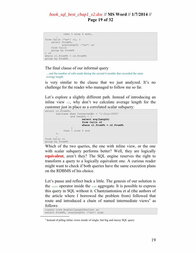
then 1 else 0 end), …from Calls /*as*/ c1, ( select FromPh, avg(Length) /*as*/ av from Calls group by FromPh) c2 where c1.FromPh = c2.FromPhgroup by FromPh
The final clause of our informal query…and the number of calls made during the second 6 months that exceeded the same average length.
is very similar to the clause that we just analyzed. It’s nochallenge for the reader who managed to follow me so far.
Let’s explore a slightly different path. Instead of introducing aninline view c2, why don’t we calculate average length for thecustomer just in place as a correlated scalar subquery: select c1.FromPh, sum(case when ConnectedAt < '1-July-2005' and Length < ( select avg(Length) from Calls c2 where c1.FromPh = c2.FromPh ) then 1 else 0 end ), …from Calls c1group by FromPh
Which of the two queries, the one with inline view, or the onewith scalar subquery performs better? Well, they are logicallyequivalent, aren’t they? The SQL engine reserves the right totransform a query to a logically equivalent one. A curious readermight want to check if both queries have the same execution planson the RDBMS of his choice.
Let’s pause and reflect back a little. The genesis of our solution isthe case operator inside the sum aggregate. It is possible to expressthis query in SQL without it. Chantziantoniou et al (the authors ofthe article where I borrowed the problem from) followed thatroute and introduced a chain of named intermediate views9 asfollowscreate view AvgCallLengthPerCust as select FromPh, avg(Length) /*as*/ avgL
9 Instead of piling inline views inside of single, but big and messy SQL query
19
book_sql_best_chap1_v2.doc // MS Word // 1/7/2014 //Page 20 of 32
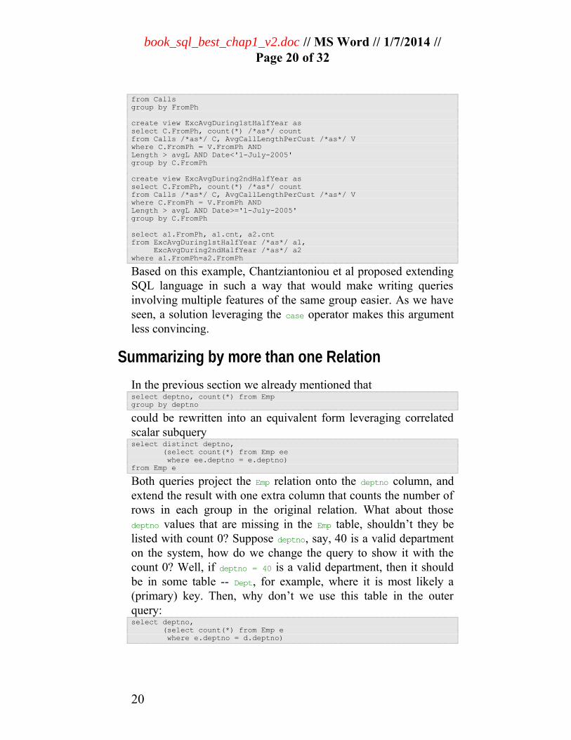
from Calls group by FromPh
create view ExcAvgDuring1stHalfYear as select C.FromPh, count(*) /*as*/ count from Calls /*as*/ C, AvgCallLengthPerCust /*as*/ V where C.FromPh = V.FromPh AND Length > avgL AND Date<'1-July-2005'group by C.FromPh
create view ExcAvgDuring2ndHalfYear as select C.FromPh, count(*) /*as*/ count from Calls /*as*/ C, AvgCallLengthPerCust /*as*/ V where C.FromPh = V.FromPh AND Length > avgL AND Date>='1-July-2005'group by C.FromPh
select a1.FromPh, a1.cnt, a2.cnt from ExcAvgDuring1stHalfYear /*as*/ a1, ExcAvgDuring2ndHalfYear /*as*/ a2 where a1.FromPh=a2.FromPh
Based on this example, Chantziantoniou et al proposed extendingSQL language in such a way that would make writing queriesinvolving multiple features of the same group easier. As we haveseen, a solution leveraging the case operator makes this argumentless convincing.
Summarizing by more than one Relation
In the previous section we already mentioned that select deptno, count(*) from Empgroup by deptno
could be rewritten into an equivalent form leveraging correlatedscalar subqueryselect distinct deptno, (select count(*) from Emp ee where ee.deptno = e.deptno)from Emp e
Both queries project the Emp relation onto the deptno column, andextend the result with one extra column that counts the number ofrows in each group in the original relation. What about thosedeptno values that are missing in the Emp table, shouldn’t they belisted with count 0? Suppose deptno, say, 40 is a valid departmenton the system, how do we change the query to show it with thecount 0? Well, if deptno = 40 is a valid department, then it shouldbe in some table -- Dept, for example, where it is most likely a(primary) key. Then, why don’t we use this table in the outerquery:select deptno, (select count(*) from Emp e where e.deptno = d.deptno)
20

book_sql_best_chap1_v2.doc // MS Word // 1/7/2014 //Page 21 of 32
from Dept d
An added bonus of having two tables in the query is that thedistinct qualifier is no longer required.
SQL is notorious for allowing multiple ways to express the samequery. Listing all the departments with the employee counts couldbe also rewritten via the outer joinselect d.deptno, d.dname, sum(case when e.deptno is not null then 1 else 0 end)from Emp e right outer join Dept dwhere d.deptno = e.deptno group by d.deptno, d.dname
If we reduce the conditional summation pattern to a simplecount(*), then the departments with no employees will count 1employee instead of 0.
Hugh Darwen’s Summarize
Hugh Darwen argued that group by with aggregation is an operator that requires two tables as the arguments, in general. The idea of introducing such an operator in SQL never caught on. Yet, in each practical situation it might be useful to double check if writing group by clauseas a one- or two- argument operator is more appropriate.
21

book_sql_best_chap1_v2.doc // MS Word // 1/7/2014 //Page 22 of 32
Which form, scalar subquery or outer join, is more performant?Surely, the answer differs between the vendors. Oracle, forexample, is better at outer join optimization than unnesting scalarsubqueries in the select clause10. Outer join from the optimizer’sperspective has almost the same rights as normal join. It can bepermuted with the other joins in the join order, it is costedsimilarly, etc. If the summarizing query is a part of the otherquery, chances are the optimizer may find the better plan when thequery is written via outer join.
10 This may certainly change as soon as Oracle implement scalar subquery unnesting.
ANSI Join Syntax
It is difficult to argue about elegance or ugliness of a certain syntax construction. You just see it or don't. Comma separated join syntax reflects the fundamental feature of Relational Algebra, which asserts the normal form for select-project-join queries. The only kind of join that escapes it (and therefore, warrants a dedicated syntax) is the outer join.
It’s not only aesthetics. It is common for production databases to have columns like CREATED_ON, or COMMENTS across many tables. In this case the NATURAL JOIN syntax is plain dangerous.
As Anthony Molinaro eloquently put it: “Old style is short and sweet and perfect. ANSI dumbed it down, and for people who've been developing for sometime, it's wholly unnecessary.”
22
book_sql_best_chap1_v2.doc // MS Word // 1/7/2014 //Page 23 of 32
Interval Coalesce
Normally, the shorter the problem statement is, the simpler itsformal expression in SQL. There are notable exceptions, andinterval coalesce11 is one of them. Given a set of intervals, return the smallest set of intervals that cover them.
This deceptively simple formulation, however, leaves a pile ofquestions. First, what is the intervals table? This one is easytable Intervals ( x integer, -- start of the interval y integer -- end of the interval);
ALTER TABLE IntervalsADD CONSTRAINT ends_ordering CHECK( x < y );
Perhaps, the from and to, or maybe, start and end column namesmay sound more appropriate. Unfortunately, they are SQLkeywords.
Next, what is the concept of one interval covering the other? Easy:interval is a set of points between the interval endpoints x and y.What about the endpoints, are they included into interval or not?For our purpose, let’s agree that both x and y belong to interval setof points, in other words, intervals are closed from both ends.Open and half-open intervals require careful reexamination of allthe inequality predicates in the query which we are going to write.Therefore, formally: A = {p|x≤p≤y}. Finally, interval A coversinterval B when B is subset of A: B⊆A.
Armed with these definitions, we are ready to write the query. TheIntervals table is the only candidate to be placed into the queryfrom clause, but there is a catch. If we just select some intervalsout of the set we have, we won’t get the answer. Think about aneasy case of two overlapping intervals. The answer to the query isan interval whose endpoints are combined from different records.Therefore, we need a selfjoin:select fst.x, lst.y from Intervals fst, Intervals lstwhere fst.x < lst.y
11 There are two terms in the literature. “Developing Time-Oriented Database Applications in SQL” by R. Snodgrass uses interval coalesce, while “Temporal Data and The Relational Model” by C. Date et al calls it interval packing.
23
book_sql_best_chap1_v2.doc // MS Word // 1/7/2014 //Page 24 of 32
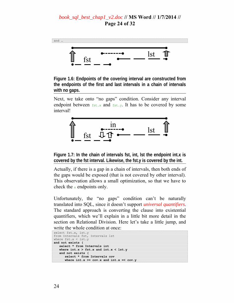
and …
Figure 1.6: Endpoints of the covering interval are constructed fromthe endpoints of the first and last intervals in a chain of intervalswith no gaps.
Next, we take onto “no gaps” condition. Consider any intervalendpoint between fst.x and fst.y. It has to be covered by someinterval!
Figure 1.7: In the chain of intervals fst, int, lst the endpoint int.x iscovered by the fst interval. Likewise, the fst.y is covered by the int.
Actually, if there is a gap in a chain of intervals, then both ends ofthe gaps would be exposed (that is not covered by other interval).This observation allows a small optimization, so that we have tocheck the x endpoints only.
Unfortunately, the “no gaps” condition can’t be naturallytranslated into SQL, since it doesn’t support universal quantifiers.The standard approach is converting the clause into existentialquantifiers, which we’ll explain in a little bit more detail in thesection on Relational Division. Here let’s take a little jump, andwrite the whole condition at once:select fst.x, lst.y from Intervals fst, Intervals lstwhere fst.x < lst.y and not exists ( select * from Intervals int where int.x > fst.x and int.x < lst.y and not exists ( select * from Intervals cov where int.x >= cov.x and int.x =< cov.y
24
fstlst
int
fstlst
book_sql_best_chap1_v2.doc // MS Word // 1/7/2014 //Page 25 of 32
)) and …
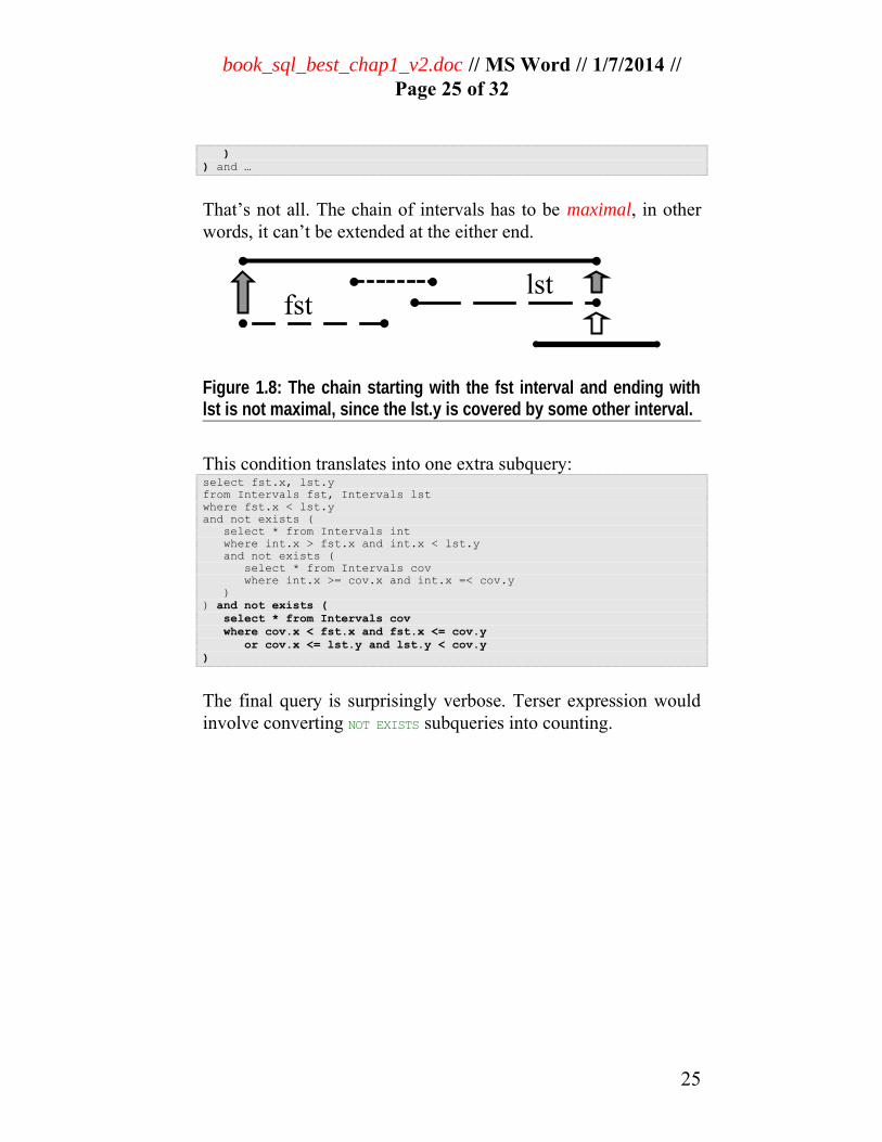
That’s not all. The chain of intervals has to be maximal, in otherwords, it can’t be extended at the either end.
Figure 1.8: The chain starting with the fst interval and ending withlst is not maximal, since the lst.y is covered by some other interval.
This condition translates into one extra subquery:select fst.x, lst.y from Intervals fst, Intervals lstwhere fst.x < lst.y and not exists ( select * from Intervals int where int.x > fst.x and int.x < lst.y and not exists ( select * from Intervals cov where int.x >= cov.x and int.x =< cov.y )) and not exists ( select * from Intervals cov where cov.x < fst.x and fst.x <= cov.y or cov.x <= lst.y and lst.y < cov.y)
The final query is surprisingly verbose. Terser expression wouldinvolve converting NOT EXISTS subqueries into counting.
25
fstlst
book_sql_best_chap1_v2.doc // MS Word // 1/7/2014 //Page 26 of 32
Which NOT EXISTS clause, because we have two? Let’s revisit bothconditions
A chain of intervals must have no gaps (fig.1.7)
A chain is maximal if it has uncovered ends (fig.1.8)
These conditions are not entirely independent, since everymaximal chain of intervals is delimited by gaps on both ends.What we need is a change of perspective.
Consider any pair of intervals fst and lst. Suppose fst.x and lst.yare not covered by other intervals. Are the fst and lst thebeginning and the end of a chain? Not necessarily, because theremight be gaps between them. Let’s shift our focus onto a set offst, lst pairs such that fst.x and lst.y are not covered by other
Is (NOT) EXISTS or (NOT) IN faster?
This is the wrong question. The EXISTS and IN subqueries are equivalent; in fact, the optimizer uses the term semijoin for both. The NOT EXISTS and NOT IN subqueries are different as faras NULL semantics is concerned, but still they are very similarso that the SQL execution engine uses the term antijoin for both. It might be argued that SQL standard should have defined them identically, leaving explicit control of NULL semantics to the end user (by means of IS (NOT) NULL predicate). History proved any attempt to get UNKNOWN value semantics right as futile, therefore it is better just to forget about NULLs and aim for elementary consistency.
26
book_sql_best_chap1_v2.doc // MS Word // 1/7/2014 //Page 27 of 32
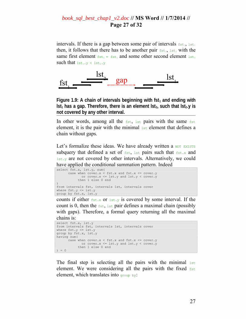
intervals. If there is a gap between some pair of intervals fst1, lst1
then, it follows that there has to be another pair fst2, lst2 with thesame first element fst2 = fst1 and some other second element lst2
such that lst1.y < lst2.y
Figure 1.9: A chain of intervals beginning with fst1 and ending withlst1 has a gap. Therefore, there is an element lst2, such that lst2.y isnot covered by any other interval.
In other words, among all the fst, lst pairs with the same fstelement, it is the pair with the minimal lst element that defines achain without gaps.
Let’s formalize these ideas. We have already written a NOT EXISTSsubquery that defined a set of fst, lst pairs such that fst.x andlst.y are not covered by other intervals. Alternatively, we couldhave applied the conditional summation pattern. Indeedselect fst.x, lst.y, sum( case when cover.x < fst.x and fst.x <= cover.y or cover.x <= lst.y and lst.y < cover.y then 1 else 0 end) from intervals fst, intervals lst, intervals coverwhere fst.y <= lst.ygroup by fst.x, lst.y
counts if either fst.x or lst.y is covered by some interval. If thecount is 0, then the fst, lst pair defines a maximal chain (possiblywith gaps). Therefore, a formal query returning all the maximalchains is:select fst.x, lst.y from intervals fst, intervals lst, intervals coverwhere fst.y <= lst.ygroup by fst.x, lst.yhaving sum( case when cover.x < fst.x and fst.x <= cover.y or cover.x <= lst.y and lst.y < cover.y then 1 else 0 end) = 0
The final step is selecting all the pairs with the minimal lstelement. We were considering all the pairs with the fixed fstelement, which translates into group by:
27
fst1
lst2 lst
1gap
book_sql_best_chap1_v2.doc // MS Word // 1/7/2014 //Page 28 of 32
select x, min(y) from ( select fst.x, lst.y from intervals fst, intervals lst, intervals cover where fst.y <= lst.y group by fst.x, lst.y having sum( case when cover.x < fst.x and fst.x <= cover.y or cover.x <= lst.y and lst.y < cover.y then 1 else 0 end ) = 0)group by x
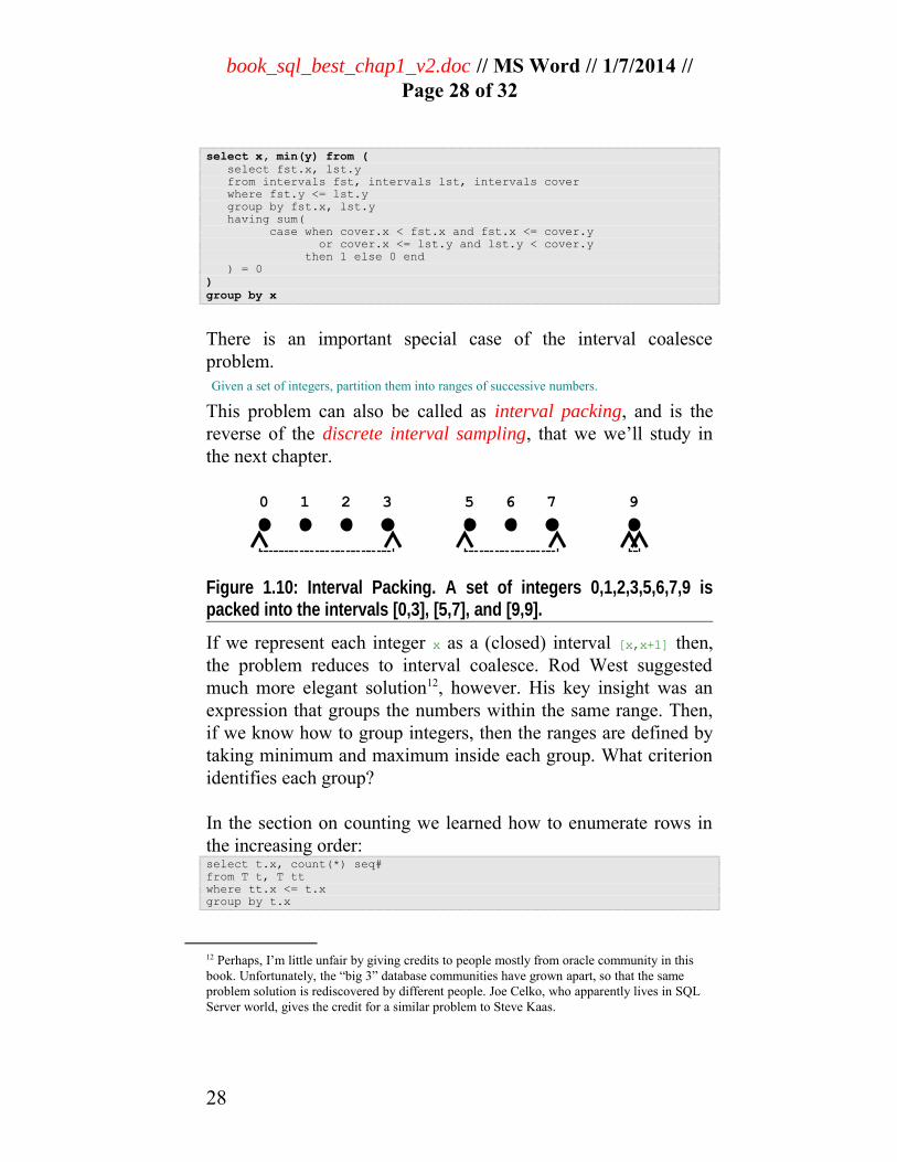
There is an important special case of the interval coalesceproblem.Given a set of integers, partition them into ranges of successive numbers.
This problem can also be called as interval packing, and is thereverse of the discrete interval sampling, that we we’ll study inthe next chapter.
Figure 1.10: Interval Packing. A set of integers 0,1,2,3,5,6,7,9 ispacked into the intervals [0,3], [5,7], and [9,9].
If we represent each integer x as a (closed) interval [x,x+1] then,the problem reduces to interval coalesce. Rod West suggestedmuch more elegant solution12, however. His key insight was anexpression that groups the numbers within the same range. Then,if we know how to group integers, then the ranges are defined bytaking minimum and maximum inside each group. What criterionidentifies each group?
In the section on counting we learned how to enumerate rows inthe increasing order: select t.x, count(*) seq# from T t, T ttwhere tt.x <= t.x group by t.x
12 Perhaps, I’m little unfair by giving credits to people mostly from oracle community in this book. Unfortunately, the “big 3” database communities have grown apart, so that the same problem solution is rediscovered by different people. Joe Celko, who apparently lives in SQL Server world, gives the credit for a similar problem to Steve Kaas.
28
0 1 2 3 5 6 7 9

book_sql_best_chap1_v2.doc // MS Word // 1/7/2014 //Page 29 of 32
It is the x - seq# expression that remains constant within eachgroup!
The rest is straightforward. We group by this expression andcalculate min and max aggregate values, which are demarcating thebeginning and the end of each intervalselect min(x), max(x) from ( select x, rank() over(order by x) seq# from T) group by x-seq
Predictably, this problem might occur in a slightly morecomplicated context. Our input relation can have one morecolumn, say name, so that integers are grouped by the name values.Rod’s solution scales up naturally to the new requirements. Theadditional grouping column just emerges in the appropriate placesselect name, min(x), max(x) from ( select x, rank() over(partition by name order by x) seq# from T) group by name, x-seq
Summary
A (naturally ordered) list of values can be enumerated via joinand grouping with aggregation, or SQL analytics query.
Use CASE operator inside the SUM aggregate function forcounting. Leveraging the CASE operator is a pragmaticalternative to counting with Indicator and Step functions.
Write complex queries as a chain of inner views nested insideeach other.
DISTINCT operator can be expressed via GROUP BY.
COUNT operator doesn’t have any arguments.
GROUP BY operator summarizes over two tables.
Use comma join syntax where possible.
29
book_sql_best_chap1_v2.doc // MS Word // 1/7/2014 //Page 30 of 32
Exercises
1. Suppose we have the two queriesselect deptno, count(*) from emp;select deptno, count(*) from empwhere sal < 1000;
Can they be combined into one?2. The query
select count(distinct ename), count(*) from emp
refers to the count function, which accepts a funnyargument with the distinct keyword. Rewrite the query insuch a way that it would utilize only “politically correct”aggregate function – the count(*) with no arguments.
3. With column expression as an argument for count()function all NULL values are ignored. Write an equivalentquery forselect count(comm) from emp
via conditional summation.4. There is no shorthand syntax for counting distinct column
combinations. Write down a query that counts the distinctnumber of the first_name, last_name in the Customers table byseparating counting and distinction in different queryblocks.
5. The having clause is redundant. Transformselect deptno from empgroup by deptnohaving min(sal) < 1000
into an equivalent form leveraging inner subquery. 6. Correlated scalar subquery can be even used within the
order by clause. Explain the purpose of the following queryselect * from emporder by (select dname from dept where emp.deptno=dept.deptno);
7. Express the indicator function 1x via standard numericfunctions abs(x) and sign(x).
8. Figure 1.6 demonstrates one way to implement themaximal chain of intervals condition. Alternatively, wecould have defined the maximal chain as the one thatmaximizes the distance lst.y – fst.x. Write the query thatformalizes that idea.
9. Write a set intersection query. Given a collection of sets,e.g. set1 = {1,3,5,7,9}
30
book_sql_best_chap1_v2.doc // MS Word // 1/7/2014 //Page 31 of 32
set2 = {1,2,3,4,5}set3 = {4,5,6,7}
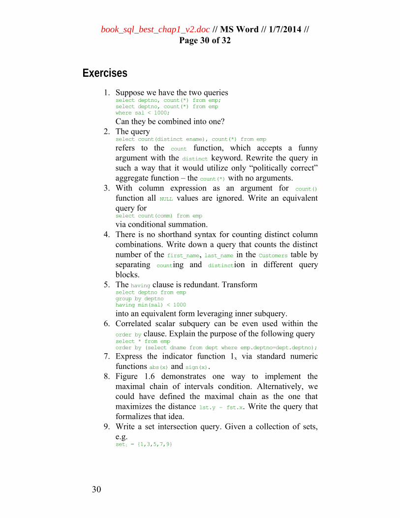
stored as a relation Sets ID ELEMENT 1 1 1 3 1 5 1 7 1 9 2 1 2 2 2 3 2 4 2 5 3 4 3 5 3 6 3 7
your query should return intersection of all the sets listed inthe relation Sets; i.e. {5} in our example. Hint: group by theelement column and count.
10. Counting words. Suppose you have a table of sentencestable Sentences { text varchar(4000);}
The SQL function instr(string, substring, startPosition)returns the position of the first occurrence of the substringin the string beginning with startPosition. Write a SQLquery that counts the number of sentences where a givenword is occurring once, twice, and so on.
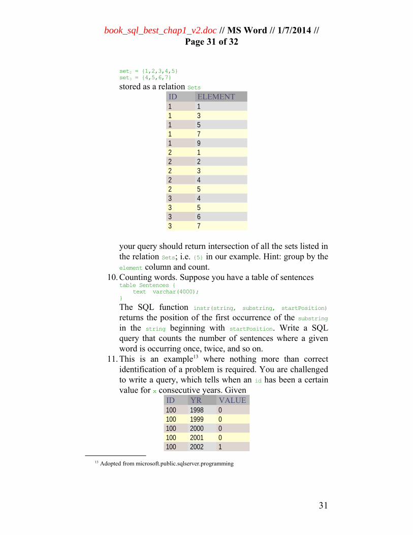
11. This is an example13 where nothing more than correctidentification of a problem is required. You are challengedto write a query, which tells when an id has been a certainvalue for x consecutive years. Given
ID YR VALUE 100 1998 0 100 1999 0 100 2000 0 100 2001 0 100 2002 1
13 Adopted from microsoft.public.sqlserver.programming
31
book_sql_best_chap1_v2.doc // MS Word // 1/7/2014 //Page 32 of 32
100 2003 0 100 2004 0 100 2005 0 100 2006 0 100 2007 0 100 2008 1 200 1999 0 200 2001 0 200 2002 0 300 2001 0 300 2002 0 300 2003 0 300 2004 0 300 2005 0
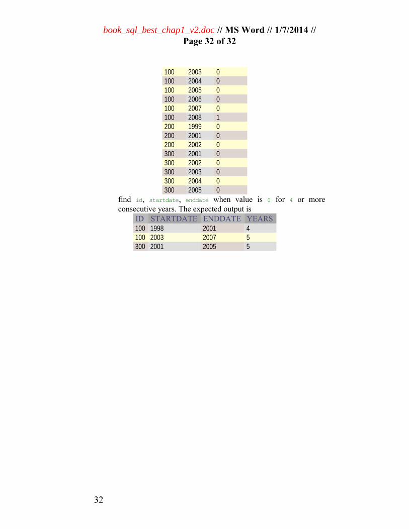
find id, startdate, enddate when value is 0 for 4 or moreconsecutive years. The expected output is
ID STARTDATE ENDDATE YEARS 100 1998 2001 4 100 2003 2007 5 300 2001 2005 5
32